investigation of the use of horizontal baffles

INVESTIGATION OF THE USE OF HORIZONTAL BAFFLES

IN A GAS-LIQUID AGITATED TANK

by

CHARLES C. FORSTER, B.S.

A THESIS

IN

CHEMICAL ENGINEERING

Submitted to the Graduate Faculty of Texas Tech University in

Partial Fulfillment of the Requirements for

the Degree of

MASTER OF SCIENCE

IN

CHEMICAL ENGINEERING

Approved

Accepted

May, 1990

CJlh.i^J ACKNOWLEDGMENTS \

The author wishes to thank Dr. Uzi Mann for his suppon, encouragement, and

guidance during the course of this work and for his assistance in writing this thesis. The

author would also like to thank Drs. R. R. Rhinehan and R. W. Tock for serving on the

thesis commirtee and for giving suggestions.

Special thanks are due to Mr. R. M. Spruill for his assistance in the design and

construction of the experimental system.

u

TABLE OF CONTENTS

ACKNOWLEDGMENTS ii

ABSTRACT v

LIST OF TABLES vi

LIST OF FIGURES vii

NOMENCLATURE xi

CHAPTER

1. INTRODUCTION 1

1.1 Background 1

1.2 Literature Review 4

1.2.1 Dimensionless Numbers Used in Analysis of Mixing Operation 6

1.2.2 Agitation Power 8

1.2.3 Hydrodynamics of the Gas-Liquid Agitated Tank 10

1.2.4 Gas-Liquid Mass Transfer 13

1.2.5 Surface Aeration 15

2. THEORY 17

2.1 Determination of the Gas-Liquid Mass Transfer Coefficient 17

3. EXPERIMENTAL EQUIPMENT AND PROCEDURE 28

3.1 Equipment Description 28

3.1.1 Tank and Baffle Assemblies 28

3.1.2 Gas Supply 35

3.1.3 Agitator 39

iii

3.1.4 OtiierEquipment 42

3.2 Experimental Procedure 42

3.3 Analytical Procedure 43

4. RESULTS AND DISCUSSION 45

4.1 Range of Operational Conditions 45

4.2 Presentation of Data 46

4.3 Validity of the Assumptions and Accuracy of the Experimental Data 46

4.4 Effect of tiie Number of Horizontal Baffles 48

4.5 Effect of Horizontal Baffle Inclination 66

4.6 Comparison with Results of Zinzuwadia (1987) 73

5. CONCLUSIONS AND RECOMMENDATIONS 81

5.1 Conclusions 81

5.2 Recommendations 81

REFERENCES 83

APPENDICES

A. CALIBRATIONS 86

B. EQUATION DERIVATIONS AND CALCULATIONAL PROCEDURES ... 112

C. A SAMPLE CALCULATION 123

D. COMPUTER PROGRAM LISTING 134

IV

ABSTRACT

The objective of this investigation was to study horizontal baffle parameters and

determine their effect on the mixing performance of a gas-sparged agitated conta'^tor and

compare to contactors of standard design. Unlike standard baffle design, horizontal baffles

are located at tiie dispersion surface. The following horizontal baffle parameters were

investigated; the number of horizontal baffles and the inclination of each baffle. The

performance criterion to be examined was the mass transfer coefficient for a given power

input.

The experiments were conducted on a 7.5-gallon lab-scale agitated tank. The sodium

sulfite method was used to determine the mass transfer coefficient. The primary

independent variables were the impeller speed and the air injection rate. The impeller speed

and air injection rate were varied from 500 to 1500 RPM and 160 to 1280 cm^/s,

respectively.

The number of horizontal baffles and their inclination had littie effect on mixing

performance. For a gas injection rate of 160 cm^/s, contactors equipped with horizontal

baffles showed only a 25% improvement in the mass transfer coefficient compared to a

contactor of standard design. At larger gas injection rates there is little or no difference in

mixing performance for contactors of different baffle design. Results of this investigation

were compared to previous research and it was found that the design of the tank

(specifically, the horizontal baffles) is a crucial factor for improving the performance of a

contactor equipped with horizontal baffles.

LIST OF TABLES

4.1 Reproducibility of Experimental Data 47

A. 1 Spring Calibration Data 91

A.2 Motor Calibration Data 99

A.3 Pressure Bell Prover Data and Calibration Results for Large Rotameter 108

A.4 Pressure Bell Prover Data and Calibration Results for Small Rotameter 111

B. 1 Solubility of Oxygen in Water 117

C. 1 Titration Readings 125

VI

LIST OF HGURES

1.1 Standard Agitated Gas-Liquid Tank 2

1.2 Liquid Row Patterns in an Agitated Tank Equipped with a Rushton Turbine .... 3

1.3 Agitated Tank with Horizontal Baffles 5

1.4 Typical Power Curves for Non-Aerated Agitated Tanks 9

1.5 Effect of Gas How Rate and Impeller Speed on Reduced Power 11

1.6 Cavity Formation for a Six-blade Turbine Impeller (Rushton) at Increasing Aeration Numbers 12

1.7 Appearance of Different Cavity Regimes in an Agitated Contactor

without Recirculation 14

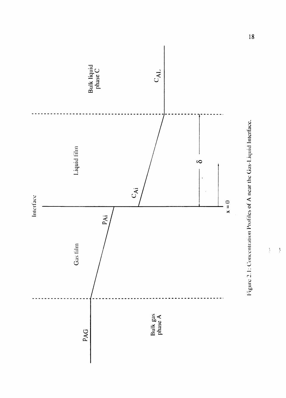
2.1 Concentration Profiles of A near the Gas-Liquid Interface 18

3.1 Schematic Diagram of Experimental System 29

3.2 Tank Details 30

3.3 Front and Top View of Horizontal Baffle Assembly 32

3.4 Top View of Horizontal Baffle Assembly 33

3.5 A View of Horizontal Baffle Mounting 34

3.6 Bolt Adjustment for Varying Baffle Pitches 36

3.7 Mounting of the Horizontal Baffle Assembly 37

3.8 Schematic Diagram of Gas Supply 38

3.9 Sparger Ring Assembly 40

3.10 Rushton Turbine Impeller (R-lOO) of 4" Size 41

4.1 Plot of KLa' versus n for Tanks Equipped with Two and Four Horizontal Baffles (Qg = 160 cm^/s) 49

vu

4.2 Plot of KLS' versus n for Tanks Equipped with Two and Four Horizontal Baffles (Qg = 530 cm^/s) 50

4.3 Plot of KLa' versus n for Tanks Equipped with Two and Four Horizontal Baffles (Qg = 900 cm^/s) 51

4.4 Plot of KLS' versus n for Tanks Equipped with Two and Four Horizontal Baffles (Qg= 1280 cm^/s) 52

4.5 Plot of KLS' versus PgA^L ^ ^ Tanks Equipped with Two and Four Horizontal Baffles (Qg= 160 cm^/s) 54

4.6 Plot of KLa' versus PgA^L for Tanks Equipped with Two and Four Horizontal Baffles (Qg = 530 cm^/s) 55

4.7 Plot of KLS' versus PgA^L fo Tanks Equipped with Two and Four Horizontal Baffles (Qg - 900 cm^/s) 56

4.8 Plot of KLS' versus PgA' L o Tanks Equipped with Two and Four

Horizontal Baffles (Qg = 1280cm3/s) 57

4.9 Plot of KLa' versus Qg for Tanks Equipped with Four Horizontal Baffles 58

4.10 Plot of KLa' versus Qg for Tanks Equipped with Two Horizontal Baffles 59

4.11 Plot of KL^'versus Qg for Tanks Equipped with Vertical Baffles 60

4.12 Plot of e versus n for Tanks Equipped with Two and Four Horizontal Baffles (Qg = 160 cm^/s) 62

4.13 Plot of e versus n for Tanks Equipped with Two and Four Horizontal

Baffles (Qg = 530 cmVs) 63

4.14 Plot of e versus n for Tanks Equipped with Two and Four Horizontal Baffles (Qg = 900 cm^/s) 64

4.15 Plot of e versus n for Tanks Equipped with Two and Four Horizontal Baffles (Qg= 1280cm3/s) 65

vm

4.16 Plot of KLS' versus n for Tanks Equipped with Horizontal Baffles at Different Inclinations (Qg = 160 cm^/s) 67

4.17 Plot of KLa' versus n for Tanks Equipped with Horizontal Baffles at Different Inclinations (Qg = 1280 cm^/s) 68

4.18 Plot of KL^' versus PgA' L ^^ Tanks Equipped with Horizontal Baffles at EHfferentInclinations (Qg= 160cmVs) 69

4.19 Plot of KLS' versus PgA' L ^ ^ Tanks Equipped with Horizontal Baffles at Different Inclinations (Qg = 1280 cm^/s) 70

4.20 Plot of e versus n for Tanks Equipped with Horizontal Baffles at Different Inclinations (Qg = 160 cm^/s) 72

4.21 Plot of E versus n for Tanks Equipped with Horizontal Baffles at Different Inclinations (Qg = 128 cm- /s) 74

4.22 Plot of KLS' versus PgA^L ^ Horizontal and Venical Baffles Obtained by Zinzuwadia (1987) 76

4.23 Plot of KLS' versus PgA^L ^ ^ Horizontal and Vertical Baffles Reproduced in This Investigation 77

4.24 Plot of £ versus n for Horizontal and Vertical Baffles Obtained by Zinzuwadia 78

4.25 Plot of e versus n for Horizontal and Vertical Baffles Reproduced

in This Investigation 79

A. 1 Motor Schematic 87

A.2 Spring Diagram and Dimensions 89

A.3 Spring Calibration Setup 90

A.4 Equipment Assembly for Motor Calibration 93

A.5 Clamp Assembly, Side View 94

A.6 Exploded View of Clamp Assembly, Top View 95

IX

A.7 Layout of Spring, Ruler, and Clamp Assembly for Motor Calibration 98

A.8 Motor Calibration Chart 104

A.9 Schematic of Bell Prover Apparatus 106

B.l Graphical Representation of Sodium Sulfite Method 113

B.2 Measured and Calculated Values 119

C. 1 Experimental Data Sheet for Sample Calculation 124

NOMENCLATURE

a Average interfacial area per unit volume of liquid, L^/L?.

a.' Average interfacial area per unit volume of dispersion, L?-/l?.

All Frequency factor for Henry's law equation (Equation B.5), L^/t^.

A| Constant used to determine liquid viscosity (Equation C. 1).

B| Constant used to determine Uquid viscosity (Equation C.l), T.

C Concentration of sodium sulfite, M/L^.

C; Local concentration of solute A, M/L^.

ÂG Concentration of solute A in bulk gas, M/L^.

ÂG Concentration of solute A in equihbrium with p ^Q, M/L^.

^;^ Concentration of solute A at liquid interface, MA- .

ÂL Concentration of solute A in the bulk liquid phase, M/L^.

C02 Concentration of oxygen in water, M/L- .

C] Constant used to determine liquid viscosity (Equation C. 1), 1/T.

D Impeller diameter, L.

D^ Diffusion coefficient of A in the liquid, L^/t.

Di Constant used to determine liquid viscosity (Equation C. 1), 1/T .

EH Henry's law activation energy (Equation B.5), L-/t^.

F Tension force applied to spring, ML/t^.

F;^ Tension force applied to spring A, ML/t^.

F3 Tension force applied to spring B, ML/t^.

FQ Tension spring preload constant, ML/t^.

XI

g Gravitational acceleration, L/t^.

gc Conversion factor.

H Henry's law constant, L^/t^.

H^ Liquid depth during tank operation, L.

H5 Stationary liquid depth, L.

k First-order reaction rate constant, 1/t.

k^ Spring constant, M/t^.

KQ Overall gas-side mass transfer coefficient, L/t.

k^ Gas-film mass transfer coefficient without chemical reaction "(denoted by °), L/t.

KL Overall liquid-side mass transfer coefficient, L/t

kL Liquid-side mass transfer coefficient with chemical reaction, L/t. 0

kL Liquid-side mass o-ansfer coefficient without chemical reaction. L/t.

L Length of moment arm, L.

U. Characteristic length, L.

m Fluid mass displaced by impeller, M/t.

N Total number of samples taken.

n Shaft rotational speed, l/t.

N j^ Molar flux of solute A, 1/L t.

Ng Aeration number.

n^ Moles of gas, M.

Npj^ Froude number.

ng in Molar flow of inlet gas, l/t.

Hg out Molar flow of outiet gas, l/t.

xu

"inert,in Molar flow of inen gas into tank, l/t.

"inert,out Molar flow of inert gas out of tank, l/t.

no^ Molar flow of oxygen, l/t.

"02,in Molar flow of oxygeii in inlet gas, l/t.

Np Power number.

NRE Reynolds number.

- WE Weber number.

P Power output of motor, ML^/t^.

p^Q Partial pressure of solute A in bulk gas phase, M/Lt^.

PAG,avg Average partial pressure of solute A in dispersion, M/Lt^.

p ^ Partial pressure of solute A at gas-liquid interface, M/Lt^.

Pfij^ Partial pressure of solute A in equilibrium with C/^Q, M/Lt" .

f*atm Atmospheric pressure, M/Lt^.

Pg Power of agitation for gassed conditions, ML^/t^.

Pfj O Partial pressure of water vapor in outiet gas, M/Lt'-

PH2O Vapor pressure of water at saturation in outiet gas, M/Lt^.

Pjnlet Inlet pressure of gas at sparger ring, Wi/Li^.

PQ Power of agitation for ungassed conditions, ML^/t^.

P Q C Pressure at rotameter operating conditions, M/Lt^.

PO^ Partial pressure of oxygen, M/Lt^.

P02,avg Average partial pressure of oxygen within dispersion. M/Lt'

P02,in Partial pressure of oxygen in inlet sparged gas, M/Lt^.

P02,out P ^ i ^ pressure of oxygen in tank outlet gas, M/Lf.

xm

PRP Pressure at which reference fluid was calibrated, M/Lt^.

Pgm Standard pressure, M/Lt^.

PsTP Standard Pressure, M/Lt^.

Qcai,STP Plo^ rate of reference (calibrated) reference fluid at STP, L^/t.

Q^ Flow rate of entrained gas, L^/t.

Qg Flow rate of sparged gas, L^/t

Qg,in ^l^t g^s flow rate, L-/t.

Qg,out Outiet gas flow rate, L^/t.

Qoc Flow rate of gas at the operating conditions of the rotameter, L^/i.

QRF ^ O ^ rate of gas indicated for rotameter reference gas, L- /t.

QsTP Flow rate of gas at standard pressure and temperature, L- /t.

R Ideal gas law constant, L^/t^T.

^AD Overall average rate of solute consumption per unit volume of dispersion, M/L- t.

AL Consumption of solute A in liquid phase, M/L^t.

^02,D (derail average rate of oxygen consumption per unit volume of dispersion,

M/L\

^02,L Consumption of oxygen in liquid phase, M/L-^t.

RR Rotameter reading, L^/t.

S Solubility of oxygen in water, M/L^.

^abs Absolute temperature, T.

T Tank diameter, L.

I Time, t.

Tamb Ambient temperature. T.

xiv

Tgyg Time-weighted average dispersion temperature, T.

tf Total elapsed time, t.

Tj Dispersion temperature at sampling time tj, T

tj Elapsed time at which sample i was withdrawn from dispersion, t.

T5 Shaft torque, ML^/t^.

Tsjj Standard temperature, T.

v Superficial gas velocity, L/t.

v Characteristic velocity, L/t.

Vj) Dispersion volume, L- .

VL Liquid volume, L^

Wj Volume of sodium thiosulfate titer used, L^.

VyJ Volume of sodium thiosulfate titer used at elapsed time tj, L .

Vj2 Volume of sodium thiosulfate titer used at elapsed time t2, L- .

X Distance from phase interface, L.

X Mole fraction of solute A in inlet gas.

^A out Mole fraction of solute A in outlet gas.

xpj o,oui Mole fraction of water in outiet gas.

inert Mole fraction of inerts in inlet gas.

Xinert,out Mole fraction of inerts in outiet gas.

XQ^ Mole fraction of oxygen.

X5 Distance of spring extension, L.

XV

Greek Symbols

a Degree of armature rotation or electrical brush lead,

a Surface tension at phase interface, M/t^.

5 Depth of penetration of solute A from the interface to the bulk liquid, L.

£ Void fraction of dispersion.

r| Cbrrelation variable,

(p Enhancement factor.

pl Density of liquid, M/L^.

PHOO Density of water, MAJ.

poc Density of gas at operating conditions of the rotameter, M/L^.

pRP Density of gas at reference condition, M/L^.

|i Viscosity of liquid, M/Lt.

M-H20 Viscosity of water, M/Lt.

XVI

CHAPTER 1

INTRODUCTION

1.1 Background

Many chemical processes involve contacting gas and liquid phases to transfer one

component from one phase into the other. An agitated gas-liquid contactor is such a system

which is used for gas absorption and gas-liquid reactions. Some industrial applications

include oxidation reactions (e.g., cyclohexane and municipal waste), hydrogenation

reactions (e.g., unsaturated glycerides), and fermentation reactions (e.g.. antibiotics,

steroids, and single-cell proteins). The tank agitator breaks the gas phase into small

bubbles which disperse in the liquid. This increases the gas-liquid contact area and

improves the absorption rate.

The design of a gas-liquid agitated tank involves two major considerations: (i) the

overall gas-liquid mass transfer rate and (ii) the power of agitation. Secondary

considerations include solids suspension, heat removal, blending of reactor contents, etc..

but these are usually satisfied when the design is satisfactory for mass transfer (Uhl and

Gray, 1966).

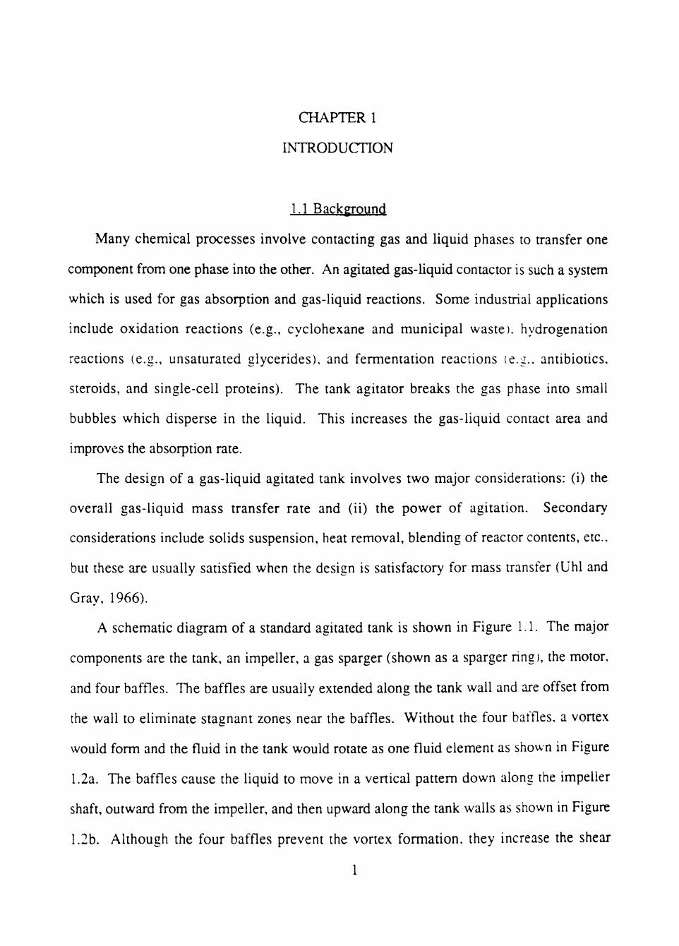
A schematic diagram of a standard agitated tank is shown in Figure 1.1. The major

components are the tank, an impeller, a gas sparger (shown as a sparger nng), the motor,

and four baffles. The baffles are usually extended along the tank wall and are offset from

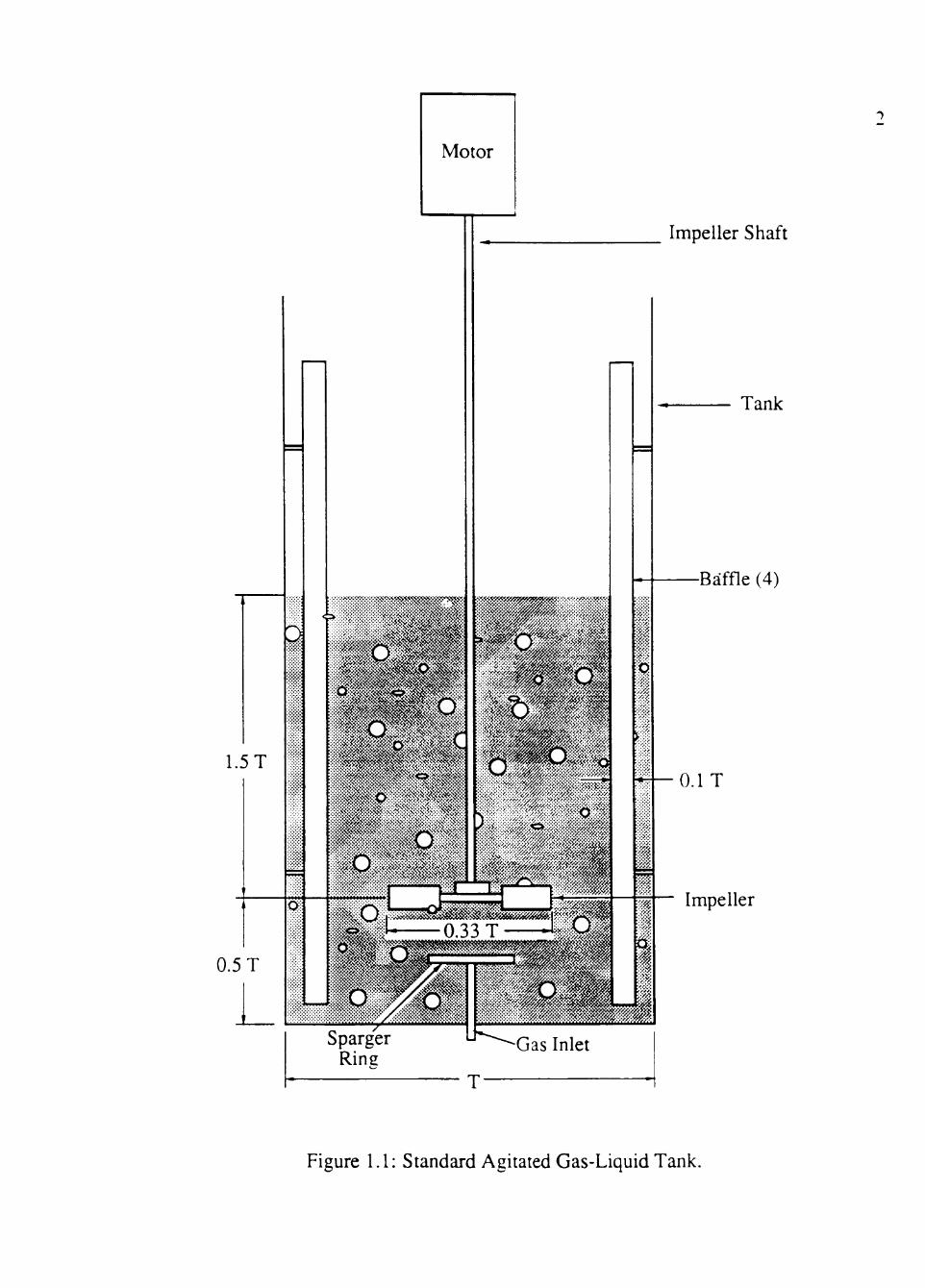
the wall to eliminate stagnant zones near the baffles. Without the four baffles, a vonex

would form and the fluid in the tank would rotate as one fluid element as shown in Figure

1.2a. The baffles cause the liquid to move in a vertical pattern down along the impeller

shaft, outward from the impeller, and then upward along the tank walls as shown in Figure

1.2b. Although the four baffles prevent the vortex formation, they increase the shear

1

Impeller Shaft

Tank

1.5 T

0.5 T

Baffle (4)

0.1 T

Impeller

Figure 1.1: Standard Agitated Gas-Liquid Tank.

^hMftMMA*M«*M**«*M*Md*MM**MM*M*M**AM«A**

mmmmmmmmmmmmtmmmllfttfmmmmtitmtmmmm

1>

X3

u

3 H c o 'yj

73

r~~'

"15 X )

^ 2

o r—

^ • « ^ ,,^-v

n

-a u CL o. • WM

3

,.> w ^ c ca H -a <u r3

« i ^

CD < C ^ ' j

r -

• - •yi

c U i

OJ

^ .^ cu ^ o u. TD • MM

3 O"

^ i ^

(N • — 1

•u u.

^ SJ)

4

forces near the impeller resulting in a higher power requirement for agitation. The vertical

baffles can cause tiie sparged gas to be shon-circuited within tiie tank. That is, tiie gas that

is injected by the sparger ring is transponed directly to the liquid surface by the liquid flow

patterns and exits the dispersion. This decreases the gas-liquid contact time and reduces

mass transfer.

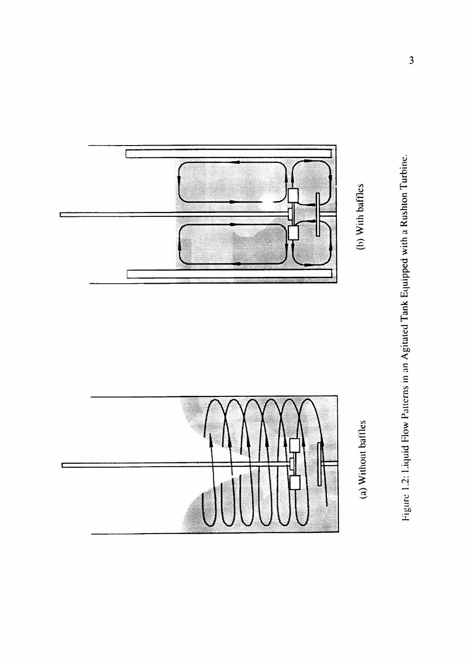
This investigation concems the use of horizontal baffles at the liquid surface instead of

the vertical baffles. In a previous work, Zinzuwadia (1987) compared the performance of

an agitated contactor equipped with horizontal baffles to the performance of a tank equipped

with venical baffles. He reponed that the horizontal baffles, shown in Figure 1.3,

prevented a vonex formation. He also reponed an 80 - 130% increase in the mass transfer

coefficient and a 33% decrease in comparison with a tank operated-with venical baffles.

He concluded that the increase in the mass transfer coefficient was mainly due to an

increase in gas holdup in the dispersion and the decrease in power requirement was due to a

lower shear near the impeller region.

The objective of this investigation is to study cenain horizontal baffle parameters and

determine their effect on the mixing performance. The following parameters were

investigated: number of horizontal baffles and the inclination of each baffle. The

performance criterion to be examined was the overall mass transfer rate for a given power

input.

1.2 Literature Review

Despite the extensive research work on mixing over more than 50 years, a significant

portion of the technology is not well understood. This is because the operation is very

complex, involving complicated flow patterns, power consumption, solids suspension.

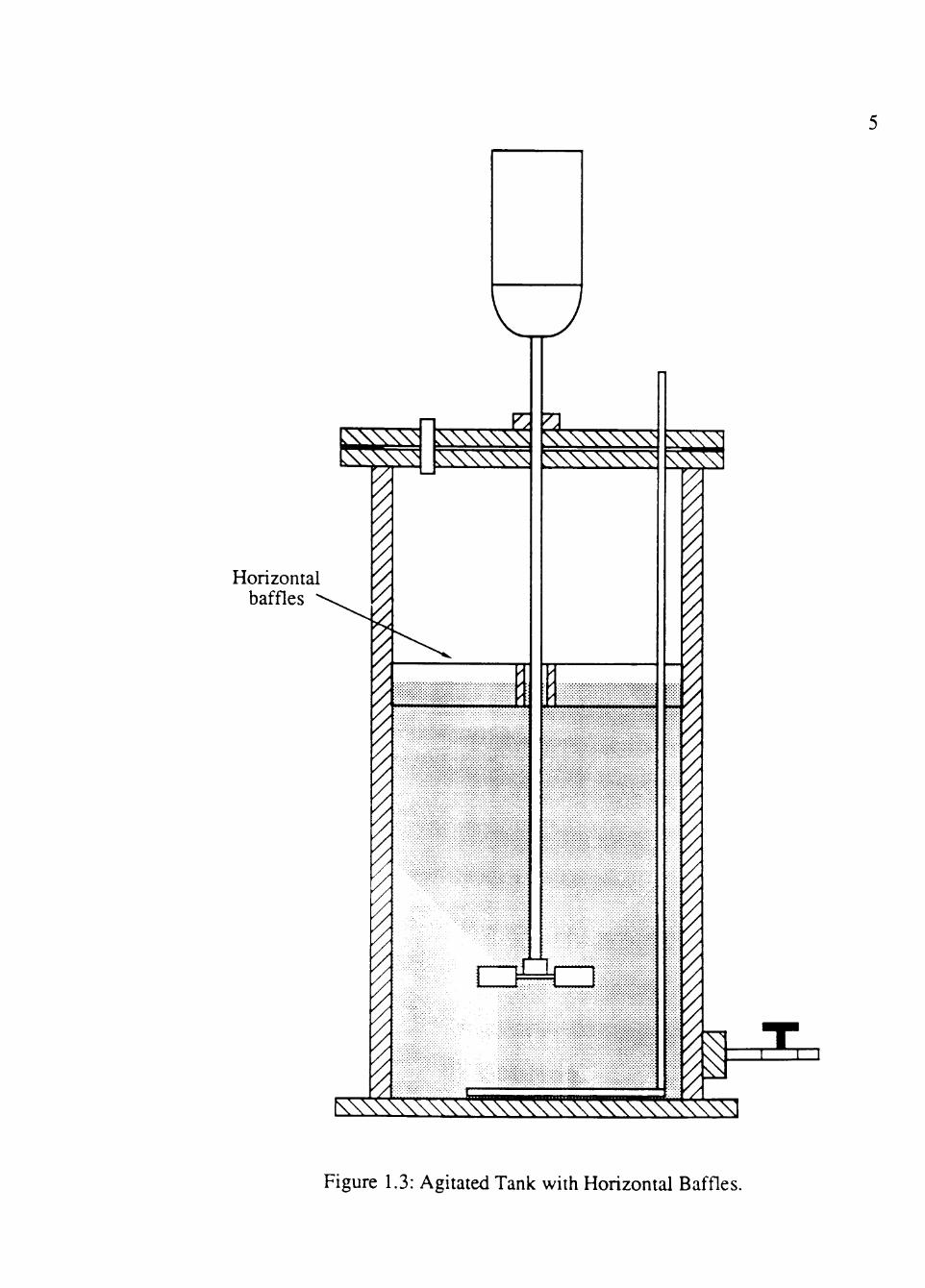
Horizontal baffles

1 r

Figure 1.3: Agitated Tank with Horizontal Baffles.

mass and heat transfer, contactor geometries, etc. A recent review of mixing technology is

given by Joshi ei al- (1982).

1.2.1 Dimensionless Numbers Used in Analvsis of Mixing Operation

At present, a mixing tank cannot be designed from fundamental concepts of liquid

motion and transport phenomena because the Navier-Stokes equations which describe the

system cannot be solved. Rather, dimensional analysis is used to help us understand the

phenomena involved with the operation. White £ial- (1934) were the first to introduce

dimensional analysis in mixing and discuss the possibility and advantage of conelating the

impeller power. Some of the commonly used dimensionless groups are reviewed below.

Reynolds number. The Reynolds number represents the ratio of inenial forces to

viscous forces. For mixing operations it is defined by,

N - 5 ^ N R E -

\^

For Reynolds numbers less than 20 the flow is laminar and for greater than 10,000 the

flow is turbulent . For Reynolds numbers between 20 and 10,000 the flow is in the

transition range.

Froude number. The Froude number represents the ratio of inenial to gravitational

forces and is defined as v^^/L^g, where g is tiie gravitational acceleration. Substituting the

characteristic length (L^ = D) and velocity (v^ = nD), tiie Froude number becomes,

In most fluid flow applications, gravitational effects are unimponant and the Froude

number is not a significant factor. The reason it appears in the dimensional analysis ot

agitated tanks is that most agitation operations are carried out with a ft^ee liquid surtace in

the tank. The shape of the surface and, therefore, the flow pattern in the vessel, are

affected by gravity. This is particularly noticeable in unbaffled tanks where vortex

formation occurs.

Power number. Fundamentally, the power number is defined as the ratio of the drag

forces on the impeller to the inenial forces within the fluid. In practice, the power number

is the ratio of the power supplied by agitation, PQ, to the rate of momentum produced by

the rotating impeller and is defined as Po/mv^^, where m is the mass of the fluid displaced

by the impeller per unit time (pinD^) and v^ is a characteristic velocity (nD). Thus, the

power number can be written as,

Np = - ^ • Pin^D^

The power number for fluid agitation is analogous to the drag coefficient in fluid flow

analysis.

Aeration number. The aeration number is a ratio of the gas feed rate to the impeller

pumping rate and is defined as,

N = ^

The aeration number is useful when a gas is injected into the liquid for conelating the

reduction in power consumption in the agitation of a gas-liquid dispersion to that of just a

bulk liquid.

Weber number. The Weber number is the ratio of inenial to surface tension forces of

the gas-liquid interface. The Weber number is defined as piv^^L^ /o and substituting for v ,

and Lj, as before, the Weber number is written,

NwE-a

It appears in conelations where the surface tension effects are important.

the tank. The shape of the surface and, therefore, the flow pattern in the vessel, are

affected by gravity. This is particularly noticeable in unbaffled tanks where vonex

formation occurs.

Power number. Fundamentally, the power number is defined as the ratio of the drag

forces on the impeller to the inenial forces within the fluid. In practice, the power number

is the ratio of the power supplied by agitation, PQ, to the rate of momentum produced by

the rotating impeller and is defined as Po/mv , . where/ m is the mass of the fluid displaced

by the impeller per unit time (pjnD^) and v , is a characteristic velocity (nD). Thus, the

power number can be written as.

P

Pin-D^

The power number for fluid agitation is analogous to the drag coefficient in fluid flow

analysis.

Aeration number. The aeration number is a ratio of the gas feed rate to the impeller

pumping rate and is defined as,

^ nD-'

The aeration number is useful when a gas is injected into the liquid for conelating the

reduction in power consumption in the agitation of a gas-liquid dispersion to that of just a

bulk liquid.

Weber number. The Weber number is the ratio of inenial to surface tension forces of

the gas-liquid interface. The Weber number is defined as piw^\^/G and substituting for v^

and L^ as before, the Weber number is written,

a

It appears in conelations where the surface tension effects are important.

8

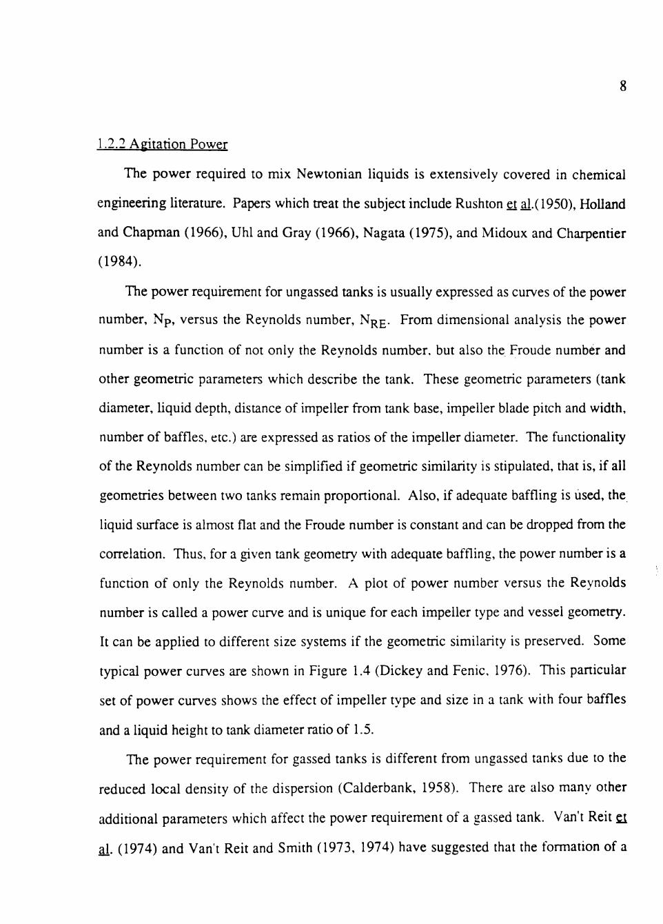
1.2.2 Agitation Power

The power required to mix Newtonian liquids is extensively covered in chemical

engineering literature. Papers which treat tiie subject include Rushton etai.( 1950), Holland

and Chapman (1966), Uhl and Gray (1966), Nagata (1975), and Midoux and Charpenrier

(1984).

The power requirement for ungassed tanks is usually expressed as curves of the power

number, Np, versus the Reynolds number, Nj^^. From dimensional analysis the power

number is a function of not only the Reynolds number, but also the Froude number and

other geometric parameters which describe the tank. These geometric parameters (tank

diameter, liquid depth, distance of impeller from tank base, impeller blade pitch and width,

number of baffles, etc.) are expressed as ratios of the impeller diameter. The functionality

of the Reynolds number can be simplified if geometric similarity is stipulated, that is, if all

geometries between two tanks remain proponional. Also, if adequate baffling is used, the

liquid surface is almost flat and the Froude number is constant and can be dropped from the

conelation. Thus, for a given tank geometry with adequate baffling, the power number is a

function of only the Reynolds number. A plot of power number versus the Reynolds

number is called a power curve and is unique for each impeller type and vessel geometry.

It can be applied to different size systems if the geometric similarity is preserved. Some

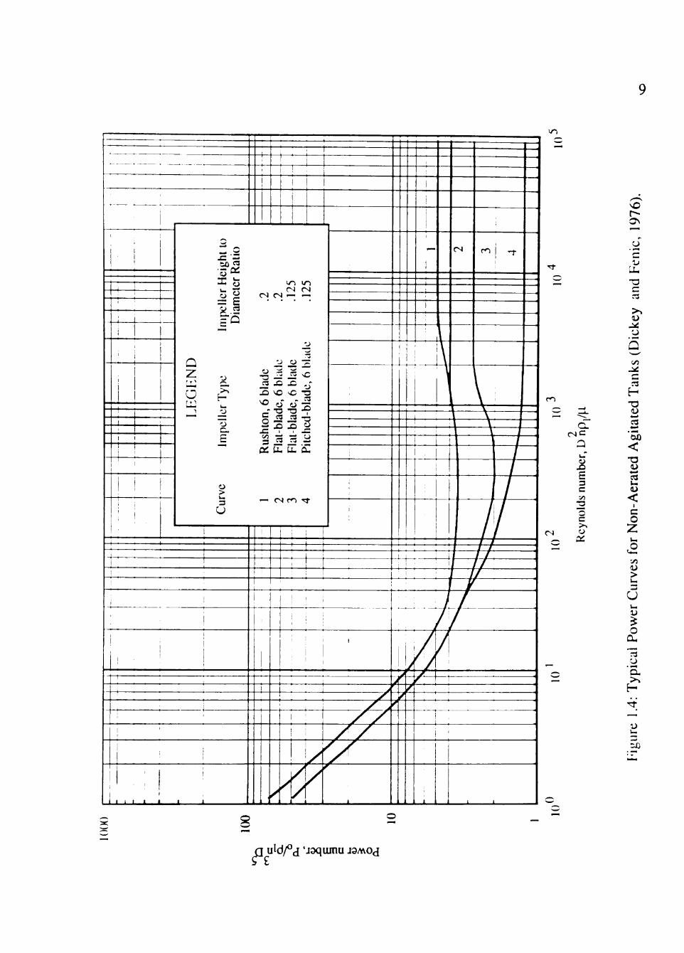
typical power curves are shown in Figure 1.4 (Dickey and Fenic, 1976). This particular

set of power curves shows the effect of impeller type and size in a tank with four baffles

and a liquid height to tank diameter ratio of 1.5.

The power requirement for gassed tanks is different from ungassed tanks due to the

reduced local density of the dispersion (Calderbank, 1958). There are also many other

additional parameters which affect the power requirement of a gassed tank. Van'i Reit £i

ai. (1974) and Van't Reit and Smith (1973, 1974) have suggested that the formation of a

^—. . .

. , .

. 1

i i

: !

'

i 1 i i 1 ' i

— i 1 ,

i i

1 ,.

1 1

1 ' 4 .1- . 1

1

. 1 1 • . i _ _

)

j

' ' 1 1 i 1 ! '

\ C

urve

Im

pell

er T

ype

Inqx

^lle

r Hei

ght t

o D

iam

cicr

Rat

io

1 R

usht

on, 6

bla

de

.2

2 Fl

at-b

ladc

, 6 b

lade

.2

3

Flat

-bla

dc, 6

bla

de

.125

4

Pitc

hed-

blad

e. 6

bla

de

.125

!

,

1 •

i '

; : j

1

1 j

j '

,

'

1

1 ^ \ 1

1 1 ' •

1 ' i 1 1 l _ l — 1 1_ _i

I ' l l '

'

;

1

t i 1 ;

• I 1 1 1

1

.

1

!

1

1 1 ^

\ \

1 : i\

1 1

CN

1

ro ^

\ — ' * • * •% - — \ ' 4 • ^ - ^

1 i l l \ 1

i ! ,

i t !

/

1 # # I I ' ' 1 i f

i i / / / t 1 1 /

! i ' 1 / / / I ' 1 1 / i

!

. - L-

1 •

, ' J 1 1

1

1 ' ' : J

i • i y

1 ' 1 X / i ' y^y

L.i, l _ ^ .

^x _±

^ f*r

/

l - _

M

f ^ 1

*

I

1 '

..J —i.

I/-)

m

<N

o

r3

~i

a. (Nt=

Oi

X) S 3 C yj

•a o c

OL

>» D

J ^ CJ

Q ^-^ iO

J ^

7i

H T3 OJ «-rf C3 * - 4

OX) <

-o u C3 U i (U

<

c o Z u« O

u^ -yj 

u o

'5, >^

5)

a uld/^'d 'Joqtunu JSMOti

10

stable vortex cavity behind the impeller blade reduces the form drag and hence the power

requirement. The stability of the vortex cavity behind the impeller blade has been found to

be a function of surface tension, electrolytic strength of solutions, foaming characteristics,

etc. Hence, the reduction in power requirement should also depend on these parameters.

Van't Reit and Smith (1974) found that the liquid viscosity influenced the stability of the

vortex cavity behind the impeller blade. Calderbank (1958) has shown that the gas holdup

is a function of the surface tension and this has been conelated by Hassan and Robinson

(1977) and Loung and Volesky (1979).

Several investigators have attempted to conelate the reduction in power requirement

with impeller speed and diameter, volumetric gas flow rate, and in some cases, the physical

properties of the system, for example Michael and Miller (1962), Clark and Vermeulen

(1963), Pharamond siai- (1975), Loiseau £iai. (1977), and Yung £t M- (1979). The

conelations derived by these investigators are reviewed by Joshi £i al. (1982).

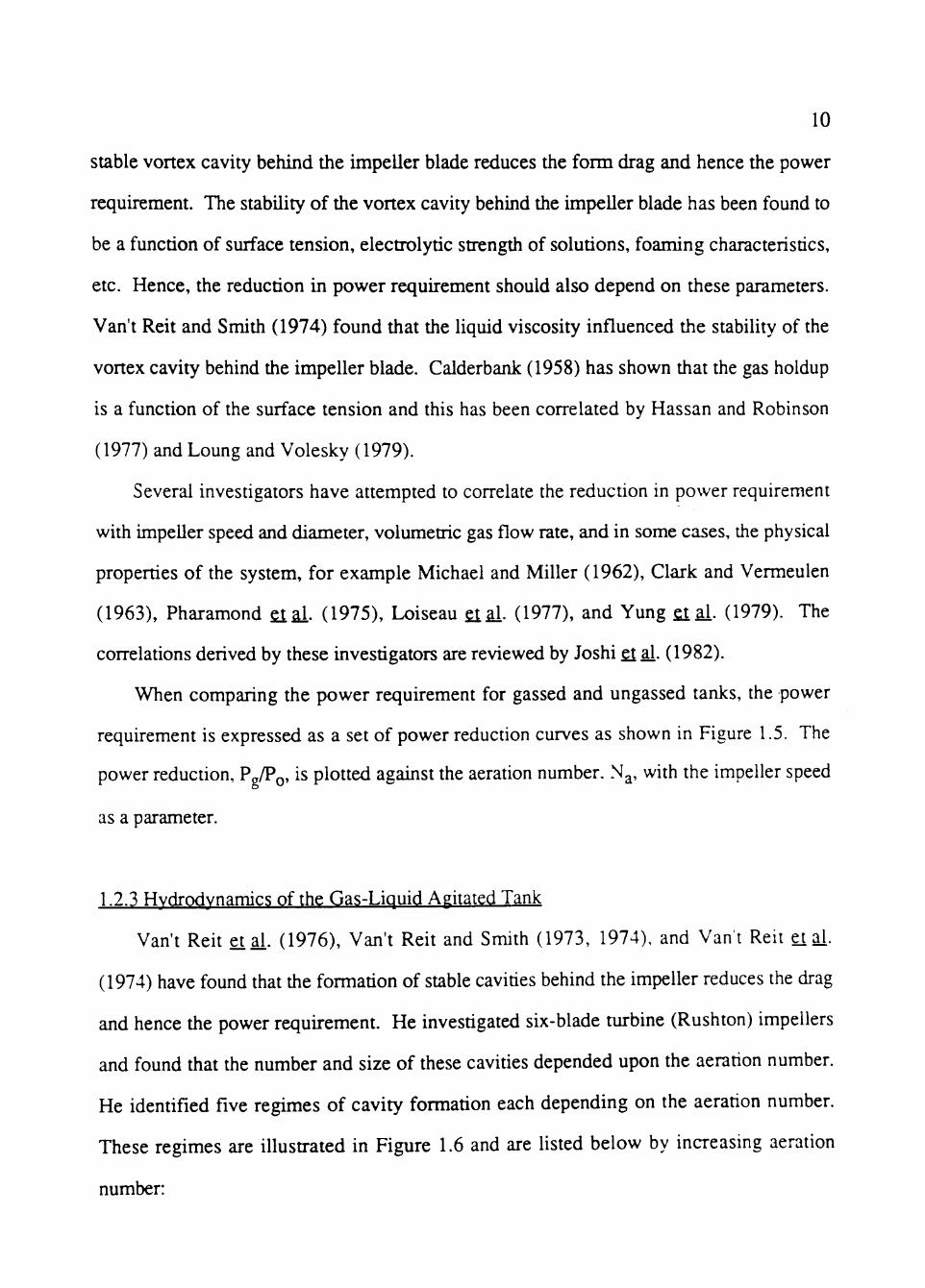
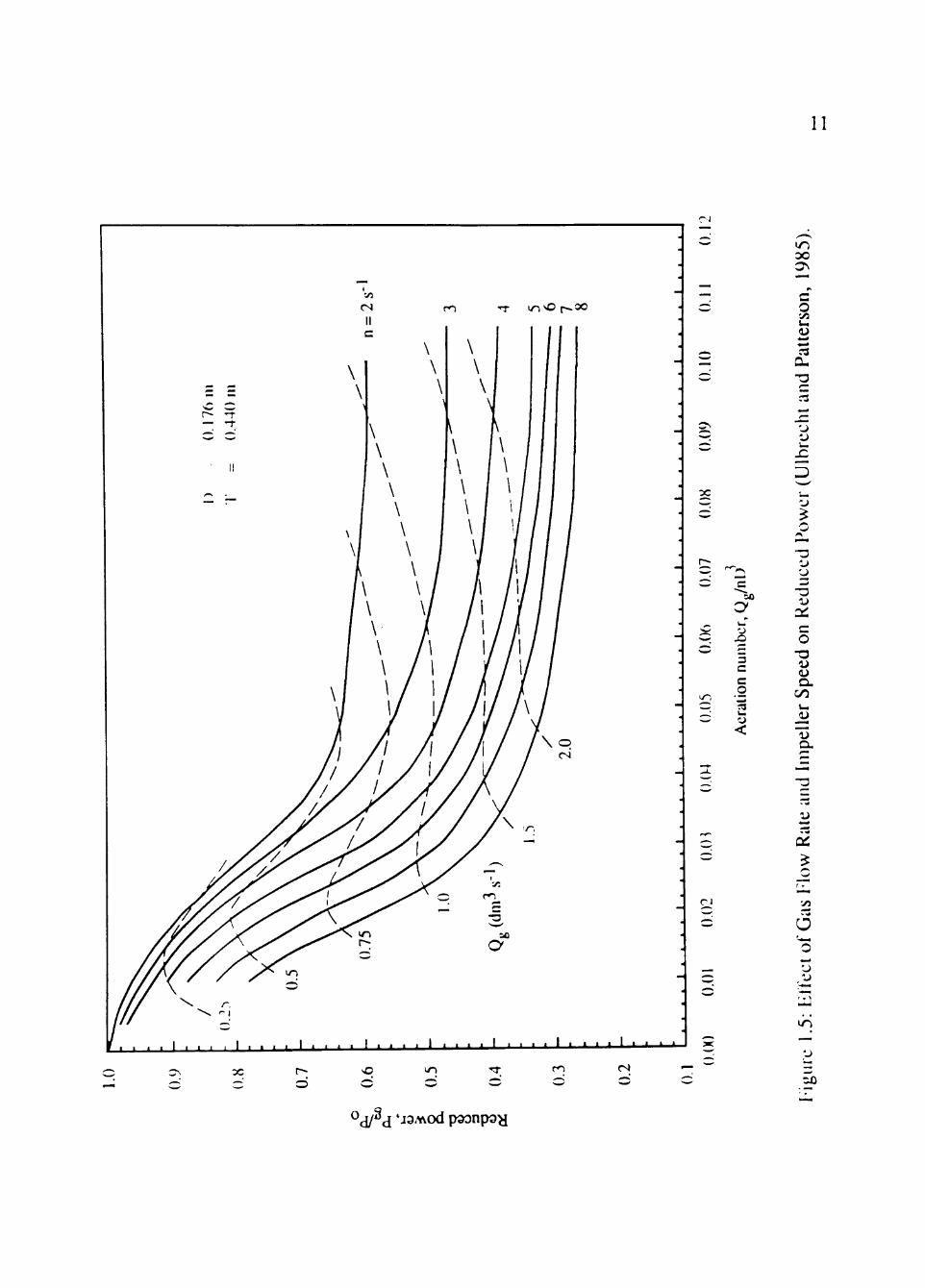
When comparing the power requirement for gassed and ungassed tanks, the power

requirement is expressed as a set of power reduction curves as shown in Figure 1.5. The

power reduction, Pg/Po> is plotted against the aeration number. N^, with the impeller speed

as a parameter.

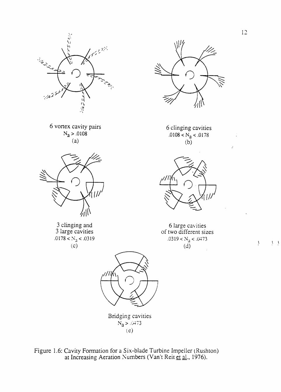
1.2.3 Hvdrodvnamics of the Gas-Liquid Agitated Tank

Van't Reit et al. (1976), Van't Reit and Smith (1973, 1974), and Van't Reit ei al-

(1974) have found that the formation of stable cavities behind the impeller reduces the drag

and hence tiie power requirement. He investigated six-blade turbine (Rushton) impellers

and found that the number and size of these cavities depended upon the aeration number.

He identified five regimes of cavity formation each depending on the aeration number.

These regimes are illustrated in Figure 1.6 and are listed below by increasing aeration

number:

11

rJ

_ -x

" ' - > "c

w u

JD /

nun

c _g ?: k .

<

un oo ON —~

^ r^

o -ys U i

« ^ : Cu •o

r -

ri ^^ '.J iJ u.

SL - :D

~ - u« --) ^ / , ^ n

* i ^ *

-a "-> ' v j

-

Red

r"

o

eed

Q. 00

b«

JJ 13 a.

C )

P

lis

5)

°cl/^d 'J3'^od psonpoy

12

6 vonex cavity pairs >.0 (a)

Na > .0108

3 clinging and 3 large cavities

.0178<N3<.0319 (C)

Bridging cavities

le) Na > .13473

6 clinging cavities .0108

/"fC 1^

<Na< (b)

^

o , / / ^

.0178

4 "*•*"* \

^u>J

6 large cavities of two different sizes

.0319<N3<.0473 (d)

\ \

Figure 1.6: Cavity Formation for a Six-blade Turbine Impeller (Rushton) at Increasing Aeration Numbers (Van't Reit et ai-, 1976).

13

a) Six pairs of vortex cavities; one pair for each blade,

b) Six clinging cavities,

c) Three large cavities alternately positioned witii respect to three clinging cavities, the

"3-3 configuration,"

d) Two groups of three large cavities with larger and smaller cavities on successive

blades, and

e) Three bridging cavities arranged symmetrically and filling the space between

alternate blades. This condition is also called impeller flooding.

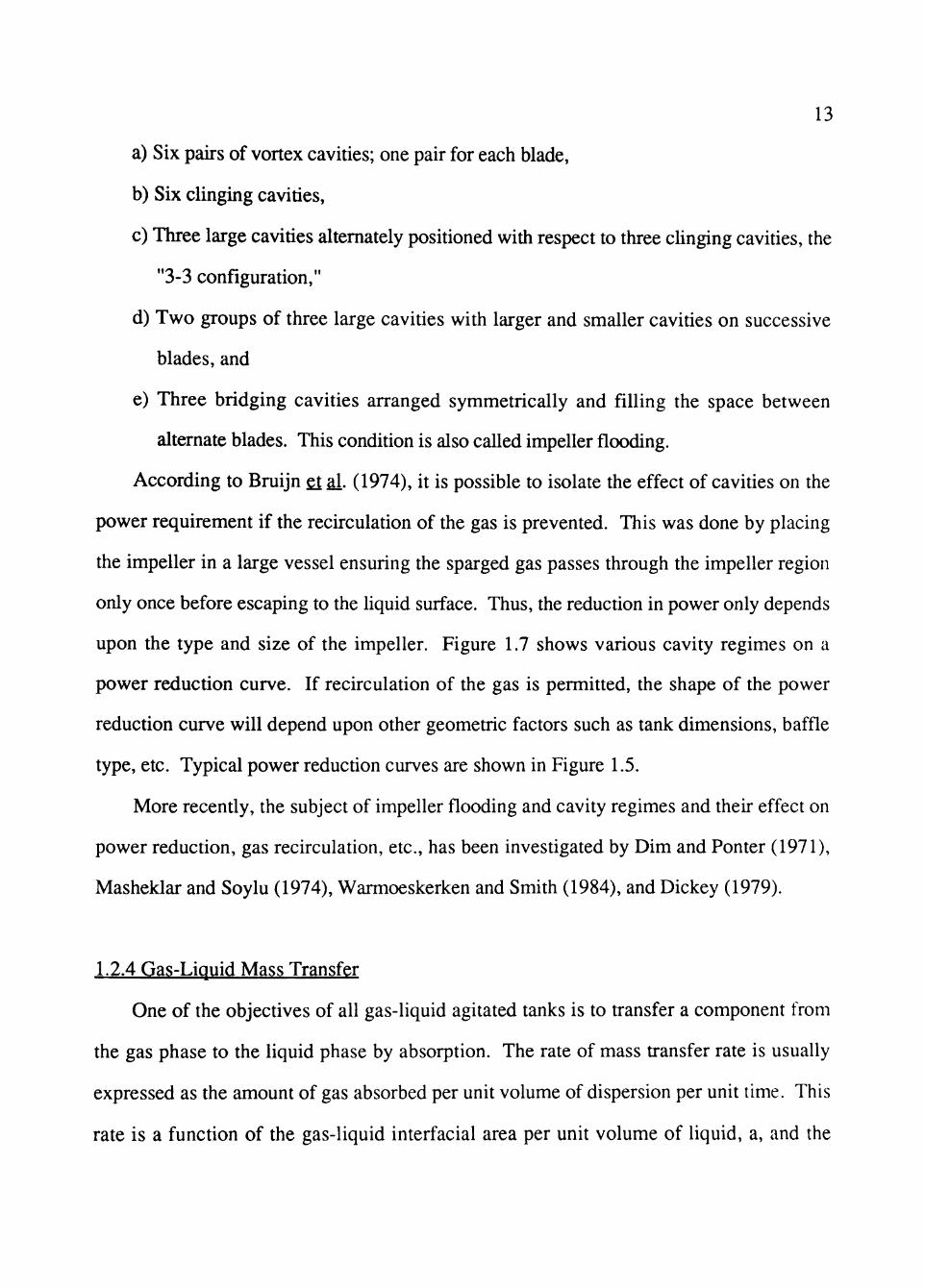
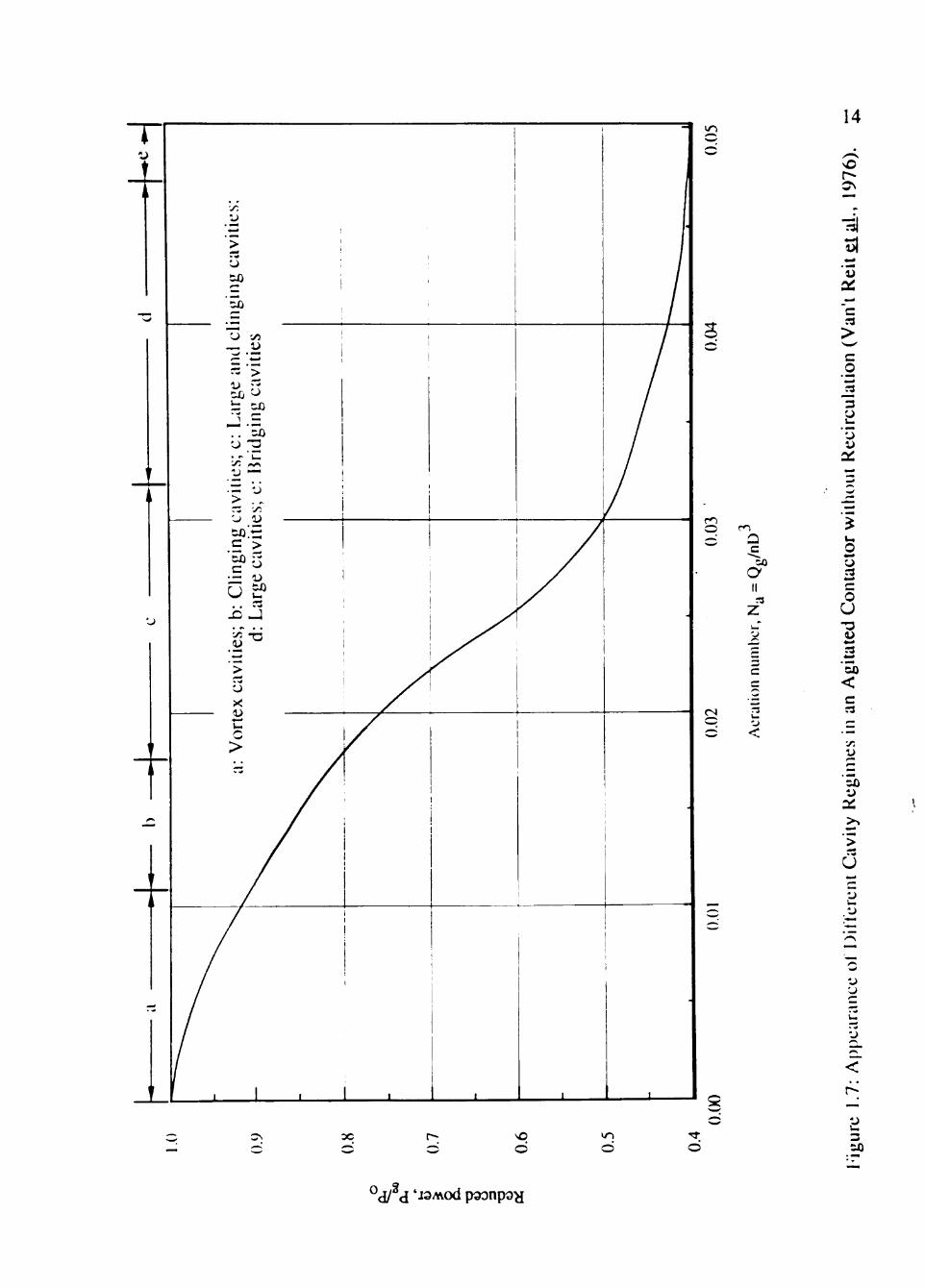
According to Bruijn £l al- (1974), it is possible to isolate the effect of cavities on the

power requirement if the recirculation of the gas is prevented. This was done by placing

the impeller in a large vessel ensuring the sparged gas passes through the impeller region

only once before escaping to the liquid surface. Thus, the reduction in power only depends

upon the type and size of the impeller. Figure 1.7 shows various cavity regimes on a

power reduction curve. If recirculation of the gas is permitted, the shape of the power

reduction curve will depend upon other geometric factors such as tank dimensions, baffle

type, etc. Typical power reduction curves are shown in Figure 1.5.

More recently, the subject of impeller flooding and cavity regimes and their effect on

power reduction, gas recirculation, etc., has been investigated by Dim and Ponter (1971),

Masheklar and Soylu (1974), Warmoeskerken and Smith (1984), and Dickey (1979).

1.2.4 Gas-Liquid Mass Transfer

One of the objectives of all gas-liquid agitated tanks is to transfer a component from

the gas phase to the liquid phase by absorption. The rate of mass transfer rate is usually

expressed as the amount of gas absorbed per unit volume of dispersion per unit time. This

rate is a function of the gas-liquid interfacial area per unit volume of liquid, a, and the

m 14

sO

151

"c >

C

_o _^ 3 k.

a:

r*l O

^

<N

*

^ M

:~

r-i

c i O

a II a

z u«

^ • ^

c c

•^ r3

'-» <

> >

tor

CJ r3

c O U -o :3

• « M

CO < c r3 • M

cm C

avit

y R

egim

es i

k_ 'J

y

u

<

d vn

d d 3 5X)

°d/^<I 'J3Avod p^onpo^i

15

concentration driving force, ( C ^ Q - C^^^). The overall liquid-side mass transfer

coefficient, KL, is defined by the relationship,

NA = KL a (CAG - CAL),

where C^G is the concentration of solute A in the bulk gas and C^L is the concentration of

the solute in tiie bulk liquid.

Usually the performance of an agitated contactor is determined by study of the product

of the interfacial area and the mass transfer coefficient, written as KLa. One of the most

common methods to determine KLa is the sodium sulfite method originally used by Cooper

et al- (1944). This method has been used by Chain and Gualandi (1954), Elswonh eiai-

(1957), and others because it is simple, inexpensive and the results are rehable. Using this

method, the rate of gas absorption is determined for a known driving force, thus the

product KLa can be calculated.

1.2.5 Surface Aeration

Surface aeration is the entrainment of gas into the liquid from the freeboard above the

liquid surface. In most applications surface aeration is ignored when designing a contactor.

In the fermentation industry where the effects of surface aeration are important, contactors

are designed to enhance surface aeration. Calderbank (1959) pointed out that surface

aeration increases the gas hold-up in the contactor, thus increasing the gas-liquid interfacial

area. Despite this, very few studies on the effects of surface aeration and power

requirement have been published.

Matsumara et ai. (1977) studied surface aeration rates with a Rushton turbine in a tank

with four vertical baffles. The following conelation was proposed,

- ^ = 1.913 X 10-3 (^)-2.2 (JlDi^O.. ("_!5!P1)..38 ( " ^ ^ 7 ^ 6 . 4 , 1 - ri nD HH,O O S '

16

where r\ = QE/ (QE + Qg), and Qg is the volumetric flow of the sparged gas and Q^ is the

volumetric flow rate of the entrained gas.

Metha (1970) has studied mass transfer coefficients enhanced by surface aeration. He

obtained values of interfacial area, a, and liqiud-side mass transfer coefficient, KLa, using a

six-blade Rushton turbine. The values of a and KLa were found to vary between 125 - 325

m^/m^ and .08 - .2 s*^ respectively, when Pg/Po was varied in the range of .017 to 41.11

kW/m^.

Zinzuwadia (1987) indicated that when horizontal baffles are used surface aeration

caused an increase in gas holdup and a decrease in the power requirement when compared

to tanks of standard design.

\ \

CHAPTER 2

THEORY

The objective of this investigation is to identify key parameters which affect tiie mixing

performance of gas-liquid agitated tanks with horizontal baffles. The mixing performance

is determined by considering the needed agitation power and the gas-liquid mass transfer

coefficient. The theoretical basis for the experimental methods and the calculation

procedure used in this investigation are developed below.

2.1 Determination of the Gas-Liquid Mass Transfer

Coefficient

The following analysis considers the definition of the mass transfer coefficient and

how it can be determined experimentally. This theory was first developed by Danckwerts

and Sharma (1966, 1970) and is a commonly accepted theory for gas-hquid reactions.

Consider a system where a gaseous component A is in contact with a liquid phase and

is being absorbed into the liquid phase as shown schematically in Figure 2.1. The rate of

mass transfer of solute A can be limited by the resistance at the interface. This resistance

can be modeled as consisting of two components, a gas-phase resistance and a liquid-phase

resistance, both of which are assumed to be controlled by molecular diffusion. Two

different mass transfer coefficients can be defined, one based on a liquid-side concentration

difference and the second on a gas-side concentration difference. The gas-side mass

transfer coefficient without chemical reaction, kG*, is defined as,

NA = ^C'CPAG - PAi)' (--1)

where N^ is the molar flux of A (mole/cm^ s), p^G is the partial pressure of A in the bulk

17

18

-a '5

v,^

• 1

X 3

CQ

U (U vo CO

a.

<

'J

3 "

CO

O

yt

d

<

J U;

<

-y C/5 — C3 3 .C

d a-

19

gas, and p^j is the partial pressure of A at the gas-liquid interface. The liquid-side mass

transfer coefficient witiiout chemical reaction, kL° (cm/s) is defined by,

NA = kY^C^-CAL) , (2.2)

where C^j is the concentration of solute A at the interface and C^L is the concentration of

solute A in the bulk liquid phase (mole/cm^).

Since it is difficult to measure the concentration at the interface, it is convenient to

express the flux in terms of the difference between the two bulk concentrations. This is

done by introducing an overall mass transfer coefficient. There are two overall mass

transfer coefficients each depending on the units of the driving force used. The overall

liquid-side mass transfer coefficient, KL, is based upon liquid concentration differences

and the overall gas-side mass transfer coefficient. KG, is based upon gas concentration

differences (partial pressures). They are both related and defined as follows,

NA = KL (C*AG - CAL) = KG (PAG - P*AL) • (2-3)

where C*^G is the concentration of the liquid which would be in equilibrium with the bulk

gas, p; G' ^"^ P*AL is the partial pressure of the gas which would be in equilibrium with

the bulk liquid, C^j^.

It is a well accepted assumption (Lewis and Whitman, 1924) that at the interface p/^\ is

in equilibrium with C/^L' thus, using Henry's law,

PAi = H C^i , (2.4)

where H is the Henry's law constant. We can use Henry's law to relate the bulk gas

concentration of solute A to its equilibrium concentration according to,

PAG = H C\\G • (2.5)

The liquid-side overall mass transfer coefficient can be written in terms of the individual

gas/liquid film mass transfer coefficients. Rewriting (2.3) as,

NA = KL [(C*AG - CAi) + (CM - CAL)] • (2,6)

Using (2.2) and (2.1) we can write.

20

NA . . . . . _ N A (CAI - CAL) = j ^ and (p^G - PAi) = j^« •

By substituting into (2.6) we obtain,

NA = KL[(C*AG-CAi) + ^ ] . (2.7)

Now, we can express C ^G tid C^j in equations (2.5) and (2.6) to obtain,

P* PAG _ , p _PAi ^ AG - H ^na ^Ai - ^ •

Substituting these expressions into (2.7) and factoring H we obtain.

NA = K L [ p j ( p A G - P A i ) + ^ ] = KLLPJ ^ + ^ ] . (2.8)

which reduces to.

J \__ _l_ KL - kG°H ^ kC • (2.9)

In a similar way, we obtain the gas-side overall mass transfer coefficient, KG (moles/cm^ s

kPa), as,

i = i if • ( '" For relatively insoluble gases (e.g., oxygen in water), the Henrys law constant is

very large making the first term on the right-hand side of (2.9) negligible. Thus KL is

approximately equal to kL°. Physically, this means that the liquid-side resistance is the

dominating resistance for mass transfer.

Hiegbie (1935) developed a film theory for the resistance to mass transfer from gas to

liquid. His theory states that any drop in concentration occurs in a nanow liquid region

near the interface and the concentration profile is assumed to be linear.

The mass flux of .A in the liquid can be expressed as,

where D^ is the diffusion coefficient of A in the liquid. Since the concentration profile of

21

A in the liquid film is assumed to be linear and occurs over a penetration depth of 5,

defined by Hiegbie's film theory, then the slope of the concentration profile at steady state

is constant and is given by.

dC. dx

C A J - C A T

x=0 = ^ - ^ • (2.12)

Substituting (2.11) into (2.12) we obtain,

NA = y (CAi-CAL) • (2.13)

Combining (2.13) and (2.2) gives.

, c D A kL = - ^ .

which means that the liquid-side mass n^ansfer coefficient is equal to the diffusivity of A in

tiie liquid divided by the liquid-film tiiickness.

Thus far we have considered mass transfer through the interface where there is no

chemical reaction involved. Now consider a situation where A reacts in the liquid phase to

form liquid products according to the ineversible reaction,

A(g)-HC(l) -producisd) .

Assume the reaction is first order with reaction rate constant, k, defined by,

(-rA)L = kCA

where (- ry )L is the local rate of consumption of A in the liquid phase (mole/cm^ s) and C/^

is the local concentration of A (moles/cm^).

If the reaction rate is fast in comparison with the diffusion rate, all the A reacts before

diffusing to the other side of the liquid film. In such a case the concentration profile of A in

the liquid film is not linear. Using the diffusion film theory, Danckwens and Sharma

(1966) developed an equation for the concentration profile for absorption accompanied by

fast chemical reaction. The slope of the concentration profile at the interface is given by.

dC, dx

22

(CAi - CAL) ,^,.. x-0 VDA/k

Substituting (2.14) into (2.11) we obtain.

N A = VD^k ( C A , - C A L ) • (2.15)

Now, by comparing (2.15) with (2.2) it can be seen that the term V^^k may be considered

the liquid-side mass transfer coefficient for gas absorption with chemical reaction, kL,

where,

kL = VD7k . (2.16)

The enhancement factor, (p, is defined as the ratio of the mass transfer coefficient with

chemical reaction to the mass transfer coefficient without chemical reaction. By dividing

(2.15) by (2.2) we obtain,

•P = i ^ = T Z ^ • (2.17)

When cp > 2, all the A reacts in the liquid film and CAL '^^ CAJ (Hatta, 1932, Sherwood

and Pigford, 1952, and Van Krevelen and Hoftijzer, 1948). So (2.15) can be reduced to.

NA = VDAk CAi =kLCA. • (2.18)

For a weak solute, Henry's law can be applied to relate the interface concentration to the

partial pressure of the solute. Using (2.8) and substituting into (2.18) we obtain.

NA = k L ( l f ) - (2.19)

According to Lewis and Whitman (1924), for a solute of low solubility, the partial pressure

of the solute at the interface is, for most practical purposes, equal to the partial pressure of

the solute in the bulk gas phase. This is because the gas film offers negligible diffusional

resistance compared to the diffusional resistance in the liquid film. Thus, (2.19) becomes,

NA = I C L 2 ^ . (2.20)

23

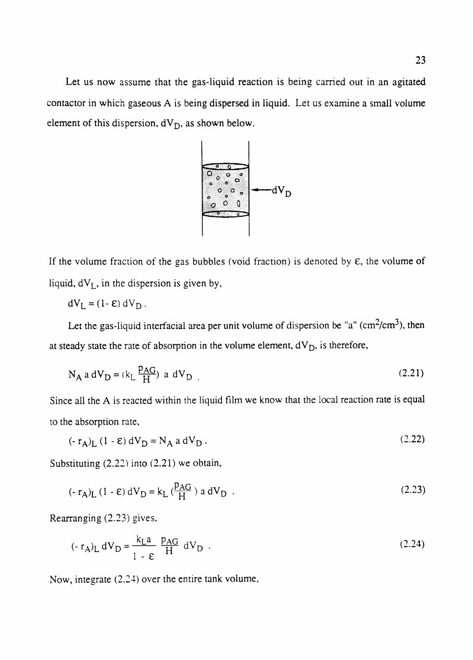
Let us now assume that the gas-liquid reaction is being carried out in an agitated

contactor in which gaseous A is being dispersed in liquid. Let us examine a small volume

element of this dispersion, dV^, as shown below.

If the volume fraction of the gas bubbles (void fraction) is denoted by £, the volume of

liquid, dVL, in the dispersion is given by,

dVL = (l-e)dVD.

Let the gas-liquid interfacial area per unit volume of dispersion be "a" (cm^/cm^), then

at steady state the rate of absorption in the volume element, dVp, is tiierefore.

NAadVD = ( k L ^ ) a d V o (2.21)

Since all the A is reacted within the liquid film we know that the local reaction rate is equal

to the absorption rate,

(-rA)L(l-e)dVD = NAadVD.

Substituting (2.22) into (2.21) we obtain,

(-rA)L(l-e)dVD = k L ( ^ ) a d V D

(2.22)

(2.23)

Reananging (2.23) gives,

^L^ PAG (- rA)L dVo =

1 - e H dV D (2.24)

Now, integrate (2.24) over the entire tank volume,

24

r

%

( - rA)LdVD = r M PAG

V'r 1 - e H

dV D (2.25)

D

The left-hand side of (2.25) is the overall rate of reaction which can be determined

experimentally. To integrate the right-hand side, the variation of all terms within the

contactor should be known. The Henry's law constant, H, is only a function of

temperature and (2.16) relates kL to the reaction rate constant, k, and to the diffusivity. DA-

At isothermal operation both k and D A are constant and they may be pulled out of the

integral.

( - r A ) L d V D = ^ H rPAG a

D

dV

V. 1 - e

D (2.26)

D

Dividing both sides of (2.26) by the total volume of the dispersion, V^, we obtain.

V D (- rA)L d V o ] = HV

rPAG a D

D

dV

V D

1 - e D (2.27)

When integrated, the left-hand side of (2.27) is the overall average rate of

A consumed per unit volume of dispersion. This quantity is denoted ( - r^ JD ^"d can be,

determined experimentally. Thus, (2.27) becomes.

( - ^A )D = r

H V D

V'r

P A G a

1 - e dV D (2.28)

D

Metha and Sharma (1971) have shown that for gas-sparged agitated tanks there is

considerable recirculation of the gas in the dispersion. Thus, the partial pressure of A can

be taken as the average partial pressure. Considering this, (2.28) becomes.

( - - X _ ^L PAG,avg 'A )D - H V D

Vr 1 - e

dVo . (2.29)

D

Now, define an average interfacial area per unit volume of dispersion as.

^ = V D

25

I r a

1 - e dVo , (2.30)

and substituting (2.30) into (2.29) we obtain.

By rearranging (2.31) we get.

, . ( - rA)DH kLa = . (2.32)

^ PAG,avg ^ ^

As mentioned above, for a fast chemical reaction compared to diffusion rate, the

liquid-side mass transfer coefficient, kL, is equal to the overall liquid-side mass transfer coefficient, KL, SO (2.32) is written as.

( -fA )D H

The term KL^' is often used to evaluate mass transfer performance in gas-liquid

agitated vessels. This equation is used as the basis for the calculation of the overall liquid-

side mass transfer coefficient.

In this investigation we determine the mass transfer rate by a chemical method based

on a reaction between oxygen and sodium sulfite a method commonly used in studies of

this type (See, for example, Elsworth si ai., 1957). In the presence of a cupric ion catalyst

(Cu"*"" ), sodium sulfite is oxidized to sodium sulfate according to,

2 SO3-2 + O2 — 2 S04-^ .

It has been shown that the reaction is fast and at sulfite concentrations above .01 molar the

conversion rate is first order in oxygen and independent of sulfite concentrations (Fuller

and Christ, 1941, and Schultz and Gaden, 1956). The local rate of reaction can be

expressed as,

(-r02)L = k C02 .

26

From stoichiometry tiie consumption of one mole of oxygen results in the oxidation of

two moles of sulfite ions. Therefore, the rate of change of sulfite concentration in the

liquid can be related to the rate of consumption of oxygen by,

d[S03-2] ^ , - dt = 2 ( - r o 2 ) L . (2.34)

Since the tank is well-mixed, the concentration of sulfite ion is uniform throughout the

tank. To convert tiie local rate of oxygen consumption based upon the liquid volume.

( • ^02 )L ' o ^ ^ based upon dispersion volume, ( - TQ )Q, the right-hand side of

(2.34) is multiphed by (ViyVL). Therefore, (2.34) becomes.

-7n

and.

d[SOv-] , , Vr> - ^ = 2( - ro2)D v7- (2.35)

-2^ 1 VL d[S03-^] ( - ^ 0 2 ) D = - 2 v ^ - ^ r ^ - (2-36)

This equation is used for calculating the rate of oxygen reaction in (2.33).

The average partial pressure of oxygen in the gas phase is determined by writing an

oxygen balance over the dispersion. In symbolic notation this can be written,

"O2 in - "02|out = ( - ^02 ) D ^ D •

Assuming ideal gas behavior, a well mixed dispersion, and rearranging we obtain.

OCT in (" ^^2 ^D ^ D P02avg =[ ^ + — o ] R T, ,g. (2.37)

^ ^ Vg,out ^g.out ^

All quantities on the right-hand side are calculated or measured, thus the average partial

pressure is calculated. For a detailed derivation of this equation refer to Appendix B.3.

This equation is used to determine the average partial pressure of oxygen in (2.33).

The Henry's law constant for an oxygen-water system is determined from oxygen

solubility data found in the literature. Since the solubility of oxygen in water is a function

27

of the temperature, the Henry's law constant is also expressed as a function of temperature.

Using the solubility data the Henry's law constant is expressed as follows,

T508.807, H = 126,361 e " ("J^ ) ' (2.38)

avg

where H is in atm l/mole. This equation is used to determine H in (2.33). For a derivation

see Appendix B.2.

CHAPTER 3

EXPERIMENTAL EQLTPMENT AND PROCEDURE

The experimental system used in this investigation was designed to allow

measurements for the determination of both the mass transfer coefficient and the power

requirement at different baffle configurations and tank operating conditions. The following

considerations were applied in the design of the system, (i) utilization of existing

equipment, (ii) ease of operation, and (iii) availability of financial resources. The final

design of the system was, for the most pan, similar to that used by Zinzuwadia (1987).

3.1 Equipment Description

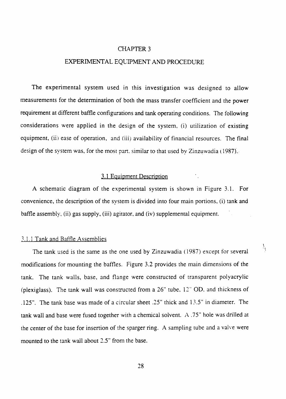
A schematic diagram of the experimental system is shown in Figure 3.1. For

convenience, the description of the system is divided into four main portions, (i) tank and

baffle assembly, (ii) gas supply, (iii) agitator, and (iv) supplemental equipment.

3.1.1 Tank and Baffle Assemblies

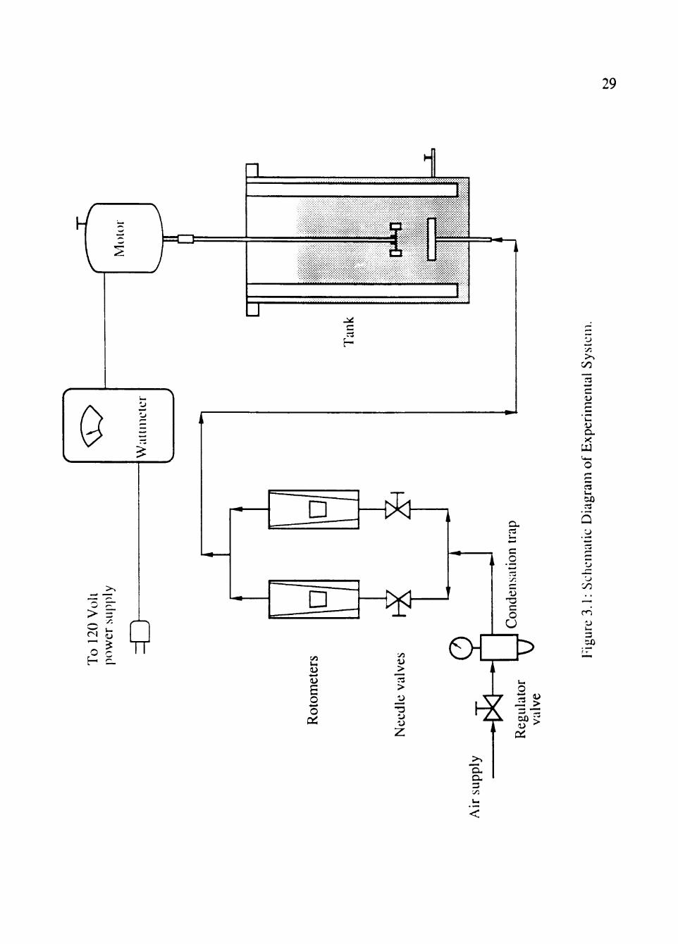
The tank used is the same as the one used by Zinzuwadia (1987) except for several

modifications for mounting the baffles. Figure 3.2 provides the main dimensions of the

tank. The tank walls, base, and flange were constructed of transparent polyacrylic

(plexiglass). The tank wall was constructed from a 26" tube, 12 " OD, and thickness of

.125". The tank base was made of a circular sheet .25" thick and 13.5" in diameter. The

tank wall and base were fused together with a chemical solvent. A .75" hole was drilled at

the center of the base for insertion of the sparger ring. A sampling tube and a valve were

mounted to the tank wail about 2.5" from the base.

28

29

>

r-1 ^" o H

"T

\r.

^ ( <—

n

0.

IJ

* * a * M M M M « M M M M *

MM***MM-rtM«te

r3

I t

s O

o

_>

>

Z

« .2

-a c o U € ^ ^

•y ;

c

Q. X

t _

r3

CJ

Si)

3

<

30

14"

12"

.25" -^ ^

26"

125" s

\

Flange

Tank wall

Vertical baffle anchor indentations

V

Sampling tube

1 K-.75"

y,±LUjj,i^yyy^yyyyyy/y;^yyyyyyyA V////////W////77>7777y^

\ \ \ \

Ji—I

YZZZm ^-^

.25"

Figure 3.2: Tank Details.

31

The flange at the top of the tank was made of a circular .5" thick circular ring, 14" in

diameter. The ring was fused flush at the top of the tank. Six .25" holes were drilled

approximately .25" from the outside edge of the flange to enable mounting of the baffles.

Four of the holes were drilled 90* apart and were used to anchor the four vertical baffles.

The other two holes were 120' to either side of one of the four other holes and were used to

suspend the horizontal baffle assembly.

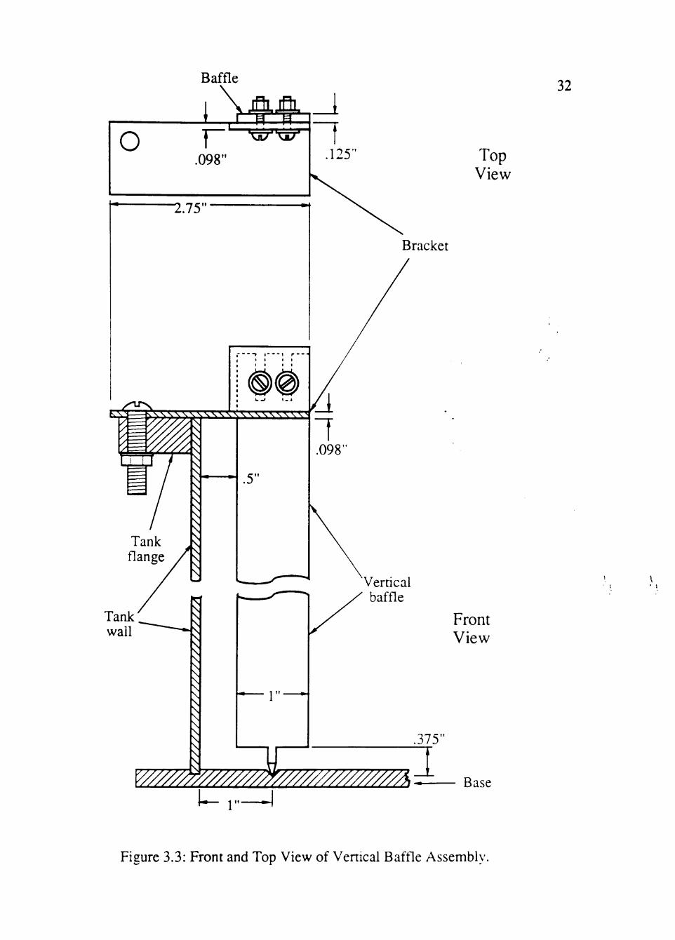
Vertical baffles were mounted individually as shown schematically in Figure 3.3.

Each vertical baffle was made of an 27" x 1" x .125" aluminum plate. The bottom of the

baffle was cut in such a way as to produce a pointed end which was inserted into an

indentation in the tank base located 1" from the inside tank wall. The top of each vertical

baffle was anchored with an L-shaped bracket as shown in Figure 3.3. The bracket was

made from a piece of 3" steel angle with approximately 1.75" of one side of the steel faces

removed. Two vertical slots, approximately 1" long, were cut into the top of each baffle to

allow mounting and adjustment of the baffle into the indentation. All metal components of

tiie vertical baffle assembly were coated with a non-oxidizing paint.

The horizontal baffle assembly was designed to allow for the use of two, three, or four

baffles, at two different baffle pitches and at different baffle submergence depths. The

design of the horizontal baffles is described in two pans, the horizontal baffle assembly

itself and the suspension unit.

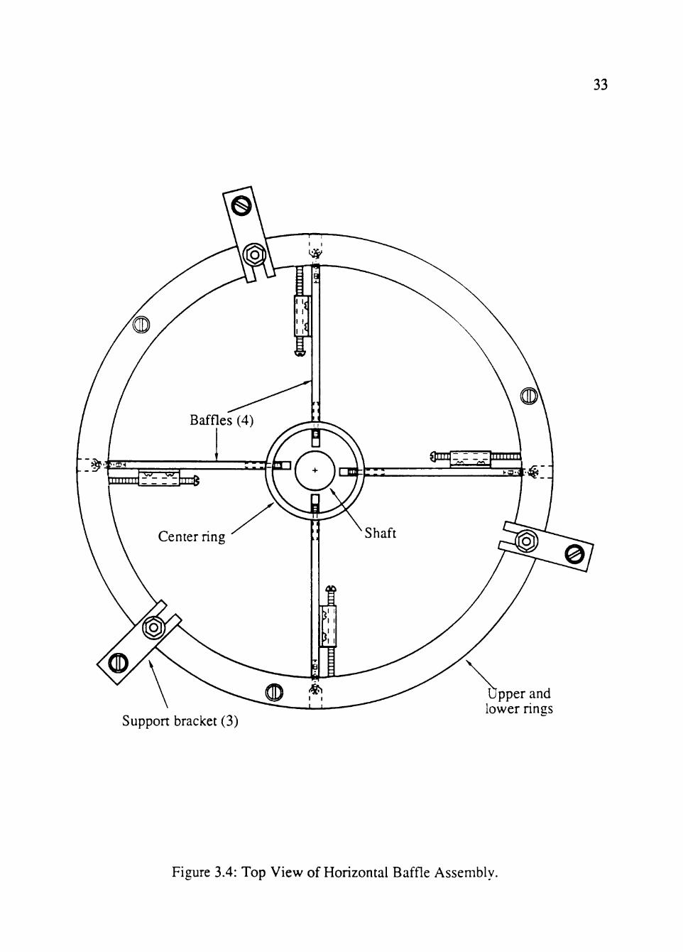
The horizontal baffle assembly consisted of an upper ring, a lower ring, a central (or

hub) ring, and the horizontal baffles themselves. A top view of the baffle assembly and

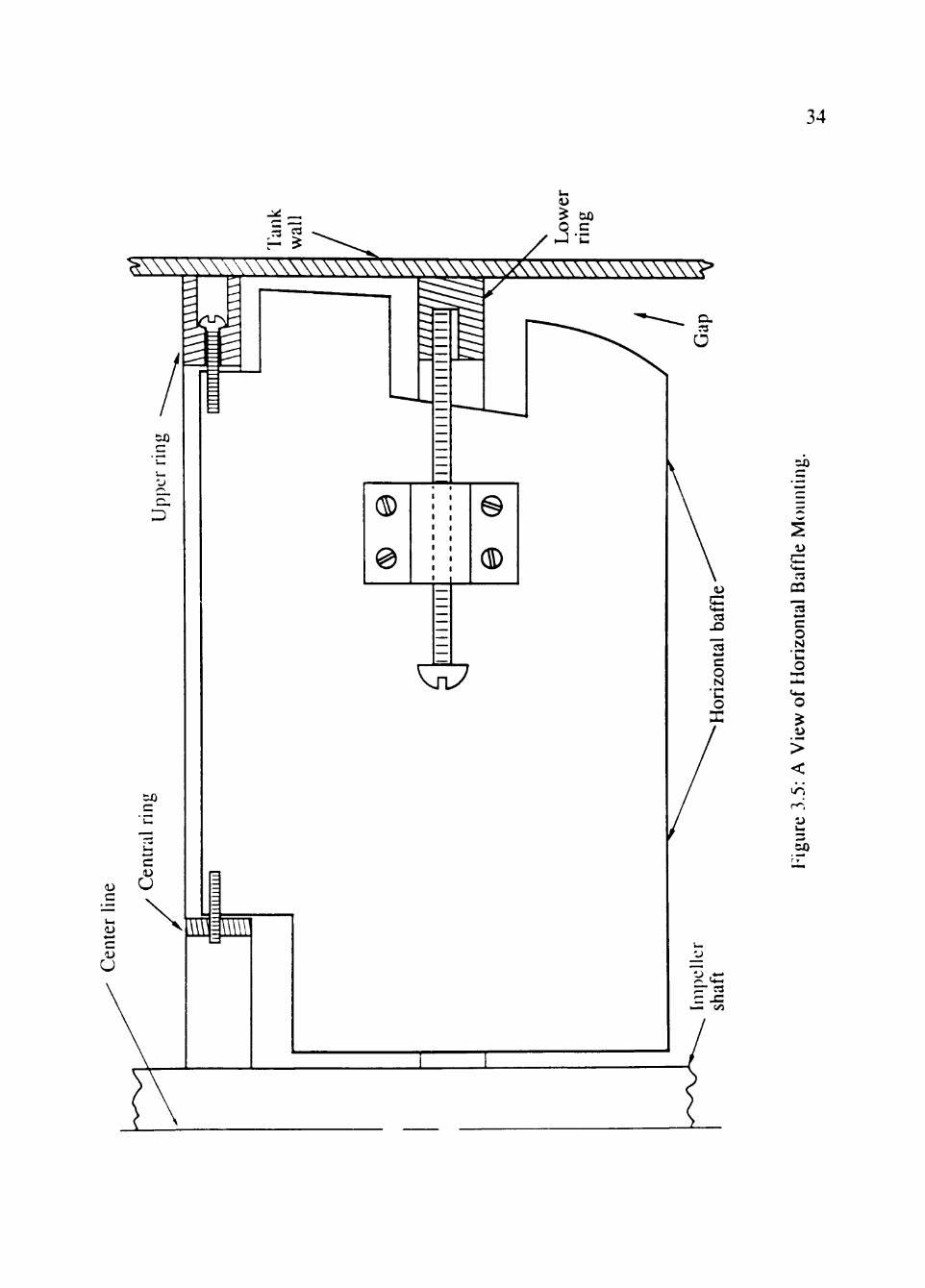
suspension is shown in Figure 3.4. Figure 3.5 shows how a horizontal baffle is connected

to the three rings. Each horizontal baffle was made from a 6" x 6" x .1875" aluminum

plate, witii the inside edge cut near the top to allow clearance for the central ring. The outer

edge of the baffle was cut in such a way to allow the baffle to be inclined at 45'. When the

baffle is oriented 90', a small gap between tiie outer edge of the baffle and the tank wall

Baffle

Bracket

32

Top View

Tank wall

Front View

.375'

mzm^m^/////////////////A^—» ase

Figure 3.3: Front and Top View of Venical Baffle Assembly

33

Suppon bracket (3)

pper and lower rings

Figure 3.4: Top View of Horizontal Baffle Assembly.

34

5 0

1>

c C3

CQ

c o N

o

> <

51)

35

develops as is shown in Figure 3.5. The baffle was connected to the central ring by a stud

which passed through one of the twelve holes drilled through the side of the ring. The

other edge of the baffle was anchored to the top ring by a small bolt. The bottom of the

baffle is held stationary by a bolt which is attached to the baffle surt'ace. This securing bolt

mates with a groove cut into the inside edge of the lower ring. Twelve round notches were

cut into the upper surface of tliis groove so that when the baffles were set at 90' the

securing bolt could be inset into the notch. This design permits the baffle to pivot at two

points allowing operation with different baffle angles.

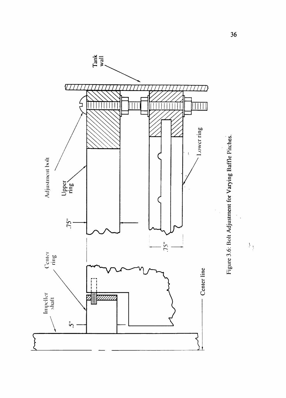
The distance between the upper and lower ring was adjustable so that different baffle

pitches could be obtained. Three long bolts located at equal distance around the rings were

used to connect the two rings. One of these adjustment bolts is illustrated in Figure 3.6.

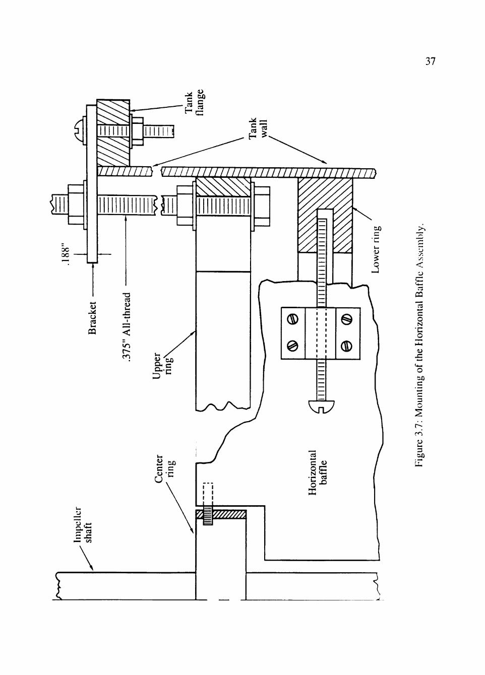
Figure 3.7 depicts the setup for suspending the horizontal baffle assembly from the

tank flange. The entire baffle assembly was suspended by three .375" all-thread bolts.

Each was attached to the upper ring by sliding the all-thread into one of the three slots.

Two nuts were tightened onto either side of the upper ring to keep the all-thread in the slot.

The all-thread and baffle assembly were supported by three brackets which were bolted to

the tank flange. A nut screwed onto the all-thread which rested on the bracket was used to

adjust the height of the baffle assembly relative to the surface of the liquid.

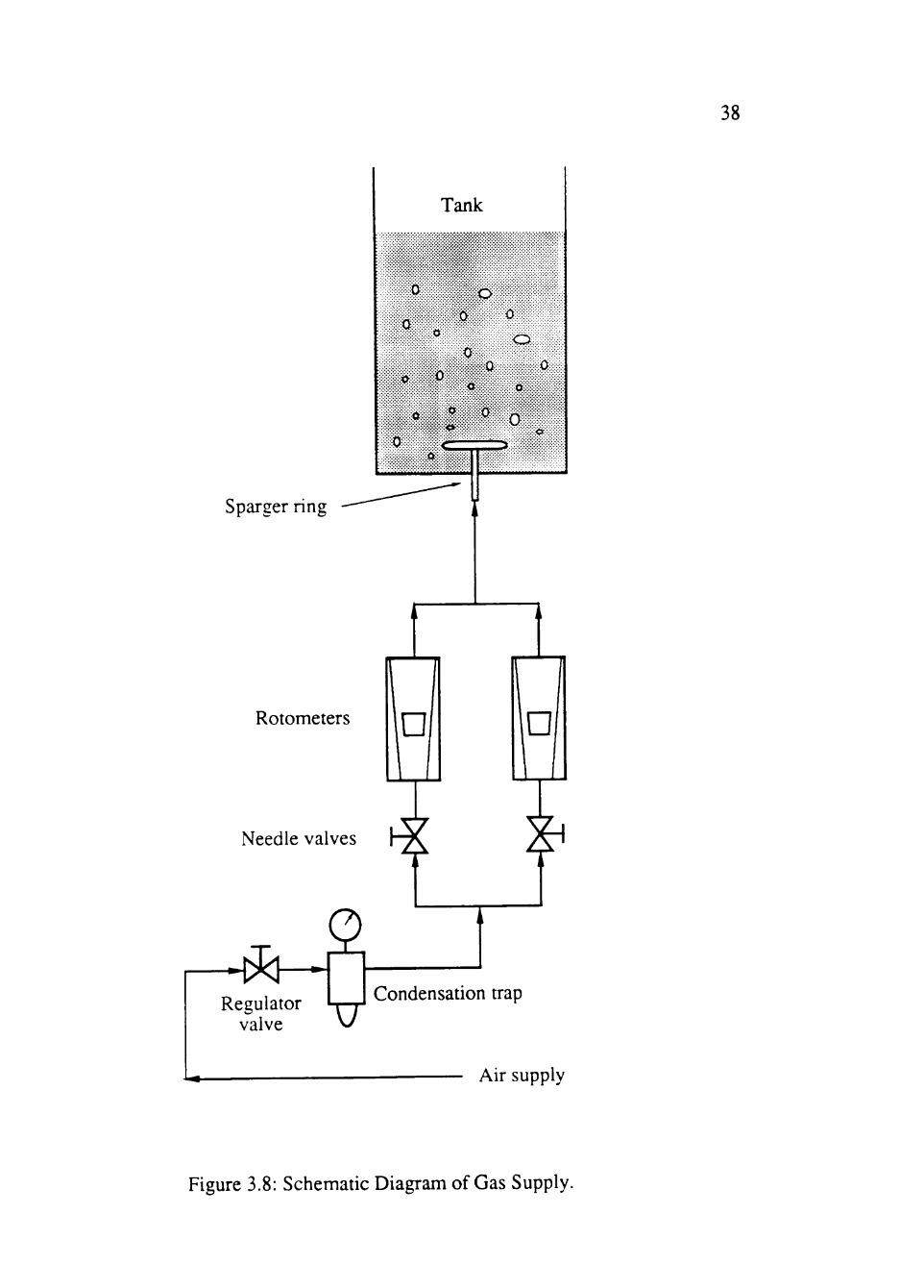
3.1.2 Gas Supply

A schematic diagram of the air supply system is shown in Figure 3.8. The

compressed air supply system (at 100 psig) served as a source of gas. The air passed

through a regulating valve and a condensation trap. The air passed through a .25" copper

tubing to a splitter and to two parallel rotameters. The air flow rate was measured by one

of the two previously calibrated rotameters (Brooks model 1110-06F1A1A or Brooks

model 1110-09-H3G1-J). The air pressure was indicated by a pressure gauge (U.S.

36

' C/5

C ( 4 -1

CQ &X)

c

>

c £

_3

<

ID l - i

OX)

37

•y.

<

C rs

QQ

c o N

•c o

o C

ax)

38

Tank

0

^ o 0 0

a * 0

0 <=

o 0

<t c

O

Sparger ring

Rotometers

Needle valves

-tJ} S

Regulator valve U

Condensation trap

Air supply

Figure 3.8: Schematic Diagram of Gas Supply.

39

Gauge Co. model Nl-11) mounted on the condensation trap. The two air lines joined and

the air passed through .625" vinyl tubing to the sparger ring supply pipe.

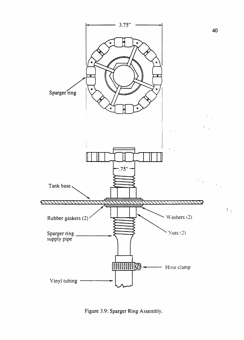
The air was injected into the tank through a sparger ring assembly shown in Figure

3.9. The air was fed into the assembly through a supply pipe constmcted from a brass rod

6.5" long and .75" in diameter. A .375" hole was drilled through the rod center and the

hole at the top was capped by soldering a small brass plate. External threads were cut to a

5.5" length of the brass rod to allow for the use of two bolts to mount the assembly to the

tank base. The sparger ring itself was constructed from eight 45° copper elbows (3/8") and

was soldered together to form an octagon. Two .03125" holes were drilled at the top of

each elbow and used as orifices for the injected air. Thus, the gas was injected from the

sparger ring into the tank through sixteen .03125" holes drilled into the copper elbows.

The sparger assembly was inserted into the hole at the center of the tank base and was held

in place with two nuts, washers, and gaskets. The ring was located 2" above the base.

3.1.3 Agitator

The agitator used was a LIGHTNIN model CV-3 with a rated power of 1/4 hp at

maximum speed of 1700 RPM. Its maximum rated cunent was 4 amps. A 120 V electric

power was supplied to the motor through a wattmeter (Weston model 310). The motor

armature was directly connected to the impeller shaft made of a .5" solid stainless steel rod

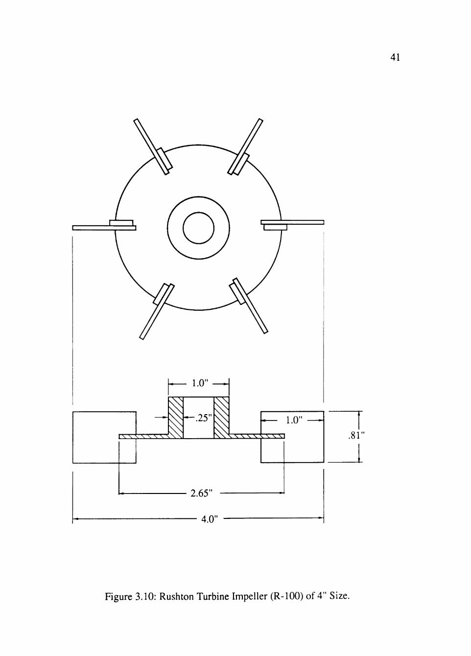
of 32" long. Two six-blade turbine (Rushton) impellers were used (LIGHTNIN type R-

100), one was 3 " and the other 4" outside diameter. The 4" impeller is shown in Figure

3.10.

The power consumption was determined by calibration of the electric motor as

described in Appendix A.

Sparger ring

40

^\\\V\\V\\\\\\\\\\\^\V\\V\VVVV\'<VVVV\VVVxVVVV\VV'v'v^

Rubber gaskets (2)

Sparger ring supply pipe

Washers (2)

Nuts (2)

Vinyl tubing

l l l l ^ Hose clamp

Figure 3.9: Sparger Ring Assembly.

41

Figure 3.10: Rushton Turbine Impeller (R-lOO) of 4" Size.

42 3.1.4 Other Equipment

A hand-held tachometer (Metron type 25A) was used to measure the impeller speed.

This measurement was taken directly from the motor armature. Two mercury

thermometers were used to measure the temperature of the dispersion. The thermometers

were immersed 76 mm into the dispersion just prior to the sampling of the tank. An

electronic timer (Kwik-set Lab-chron timer no. 1407) was used to measure the elapsed time

for each experiment. It was started when the first sample was taken from the tank.

3.2 Experimental Procedure

The effects of the following parameters on the mixer performance were investigated:

Baffle type, number of baffles and baffle inclination of horizontal baffles, impeller size, gas

flow rate, and impeller speed. The order of the experimental mns was randomly selected in

advance.

First the tank was set up to the selected configuration. Distilled water was added to the

tank until it was filled to 18" from the tank base. The motor was turned on and operated at

approximately 1000 RPM for 20 minutes to allow the motor to achieve a steady operating

temperature. The ambient temperature was recorded and the barometric pressure was

obtained from the National Weather Service and recorded. After the motor achieved a

steady operating temperature, the motor was slowed to about 500 RPM and approximately

425 grams of sodium sulfite (Fisher Cat. no. S430-3) were added to the distilled water in

the tank. For operating conditions of high gas rates and impeller speeds an additional 25

grams of sodium sulfite were poured in the tank to ensure that there was still enough

unoxidized sulfite to obtain at least five samples from the tank prior to its depletion.

The solution was agitated until the sodium sulfite had dissolved. Ten milliliters of

concentrated sulfuric acid (Fisher Cat. no. SA176-4) and 8 grams of cupric sulfate (Fisher

Cat. no. C493-500) were added to the tank.

43

Next, air was injected into the tank and the proper gas flow rate was set according to a

previously calibrated rotameter. The speed of tiie motor was adjusted to tiie selected value

by turning the variac knob at the top of the motor casing and the agitator RPM was

measured and then recorded.

Steady state was achieved by allowing tiie tank to operate for 3 minutes and then the

liquid samples were taken from tiie tank. Prior to each sample withdrawal, approximately

50 ml of liquid were drained from the the sampling port to ensure proper sampling. When

the first sample was withdrawn the timer was set and the dispersion temperature was

recorded. The sampling intervals varied from 1 to 60 minutes depending upon the

experimental conditions. For each experiment, the elapsed time between samplings was

selected so that approximately 10% of the initial sulfite concentration would be depleted

between each pair of samplings. At the end of each experiment the tank was completely

drained and washed.

3.3 Analytical Procedure

Ten 250 ml Erlennmeyer flasks were used to analyze the sodium sulfite solution

samples withdrawn from the tank during the experiment. A solution consisting of 50 ml of

distilled water, 5 ml of 30% acetic acid (Fisher Cat. no. A38-500), and 2 ml of starch

indicator solution (Fisher Cat. no. SS408-1) was added to each flask. When the sulfite

oxidation rate was rapid, 20 ml of .1 N iodine solution (Fisher Cat. no. S178-500) were

added to each flask. If the sulfite oxidation rate was slow, the iodine was added to the

flask immediately prior to sample withdrawal. During long experimental run times the

iodine solution would stand for several hours, yielding titration results that were inaccurate

by indicating a higher sulfite oxidation rate. This is due to the loss of iodine in tiie solution

by oxidation or its evaporation into the air. Thus, at impeller RPM's less than 1000 and

superficial gas velocities less than .0425 ft/s, the iodine solution was added to the flask just

44

prior to tank sampling. At aU other operating conditions the iodine was added to the ten

flasks just prior to tiie first tank sampling.

At high impeller speeds and gas rates a foam developed on the liquid surface and at

times poured over tiie top of tiie tank. It was found that by adding 10 ml of concentrated

sulfuric acid to the tank the foaming decreased. Thus, for consistency, the acid was added

to every experiment. This addition of the acid into the tank differs from the conventional

sodium sulfite method, but since sulfate ions already exist as oxidized sulfite ions in the

tank, the addition of the sulfate ions in the acid was considered not to have a significant

impact upon the sulfite oxidation rate.

A 250 ml beaker was used to collect the sulfite samplings from the tank sampling tube.

A 10 ml sample was withdrawn from this beaker by pipet and the excess immediately

dumped back into the tank. The 10 ml sample was then pipetted into one of the ten

Erlenmeyer flasks containing the iodine solution by immersing the tip of the pipet into the

solution to prevent further oxidation of the sulfite. Sometimes, upon adding the sample to

the iodine solution, the solution turned clear and no titration could be performed. When

this occurred, the sulfite concentration within the tank was greater than . 1 M and the sample

was discarded. If the iodine solution did not turn clear upon addition of the sample, the

solution was titrated with a thiosulfate solution (Fisher Cat. no. SS364-1) and the buret

levels were recorded.

CHAPTER 4

RESULTS AND DISCUSSION

Zinzuwadia (1987) found tiiat tiie use of horizontal baffles instead of vertical baffles

improved tiie performance of gas-hquid agitated tanks in terms of lower power requirement

and higher mass transfer coefficients. The objective of this investigation was to investigate

different horizontal baffle parameters and their affect on the reactor performance. These

parameters include the number of horizontal baffles, inchnation of the baffles, submergence

depth of the baffles, and impeller size.

4.1 Range of Operational Conditions

For each tank configuration several runs were conducted varying the impeller speed

and superficial gas velocity. Impeller speeds of 500, 750, 1000, 1250, and 1500 RPM

were studied and the three gas aeration rates conesponding to the superficial velocities

chosen were 0, .01, and .08 ft/s. The superficial gas velocity of .01 ft/s was chosen

because it was a gas velocity within the range investigated by Zinzuwadia. The gas

velocity of .08 ft/s was chosen because velocities of this magnitude are most often used in

industrial applications. Shortly after the experimentation started, it was found that at a gas

rate of .08 ft/s the dispersion flowed over the top of the tank at high impeller speeds.

Thus, each gas velocity was reduced 25% to .0075 and .06 ft/s, respectively. This

conesponds to gas injection rates of 160 and 1280 cm^/s at STP, respectively.

All combinations of impeller speeds and gas injection rates were attempted for each

baffle configuration. These runs were conducted in a random order. Some of the specified

operating conditions could not be achieved because the motor could not supply enough

power to obtain the desired impeller speed.

45

46 4.2 Presentation of Data

Three dependent variables were studied, the mass transfer coefficient (KLa'), the

power consumption (Pg), and the void fraction (e). The performance plot of the mass

transfer coefficient ( K L I ' ) versus the power input per unit liquid volume (Pa/yO is

commonly used to present mass transfer data (Oldshue, 1983).

To determine the effect of tiie impeller speed on tiie mass transfer coefficient, KLa' is

plotted against the Reynolds number (NRE)- Since in this investigation, the impeller

diameter, liquid density, and liquid viscosity were constant, KL^' is plotted against the

impeller speed. To determine the effect of the gas injection rate, tiie mass transfer

coefficient is plotted against the aeration number (N^). Since the aeration number is a

function of both impeller speed and gas injection rate, the impeller speed is used as the

independent variable. Similarly, a plot of void fraction versus the impeller speed is

presented, instead of versus the Reynolds number.

4.3 Validitv of Assumptions and Accuracy of the Experimental Data

Before discussing the results, it is important to discuss experimental data

reproducibility, accuracy of measurements, and the validity of the various assumptions

used in the calculations of the dependent variables.

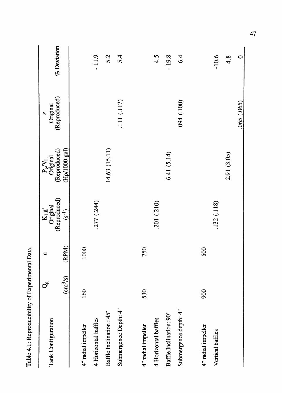
Several experimental runs were repeated during the investigation. The results and their

deviations for KLa', Pg/VL, and e are given for each of these runs in Table 4.1. The data

indicate that the values of KLa', PgA' L' ^^d e were reproducible within +12, +20, and

+7%, respectively.

The validity of the assumptions made in developing the calculations is examined.

Recall that the following main assumptions were made in the derivation in Chapter 2: (1)

the resistance to mass transfer on the gas side is negligible, (2) film theory applies, and (3)

the hquid phase is well mixed (i.e., the gas driving force is the same everywhere).

47

cd

O

c

s 0)

X

W

c o •a

I

U)

T3

fl

^ o ^ cd a.

CO

C/2

due

S

ftS '^' '^'

ble

c« H

ion

4 ->

S

fig

c o U ^ cd H

ON cs U-)

' ^

>n >o T f

oo ON

- ^

vd so o

oo ^ '

o o

ON O

t o

o

o

>o

en vo

I—I p en

0 \

Ti- o

O

oo

CO

o o o o o o

«r)

O O en IT)

o o ON

13

2

00

X )

C

in • •

c o

•a

a a . . — <

S t3 PQ

ex

Q u c £? 6

XJ

00

fe 1/3

X5 a s f2 c o N

•g X

c o

•13 a a

13

ex

O c u D s

X5 3

00

I 13

2

48

The assumptions of negligible mass transfer resistance in the gas side and the

applicability of ftim theory are supported by the fact that the experimental results obtained

by different investigators using the same method, were within + 20% accuracy of the

results of interfacial area obtained from physical metiiods (Midoux and Charpentier, 1980).

The assumption of well mixed gas phase in the liquid for runs with vertical baffle

configuration can be justified based on the experimental results of Metha and Sharma

(1971) who used agitated tanks of similar scale and geometry to the one used in this

investigation. They compared their results with measurements of interfacial area by

physical methods and showed that the assumption of a fully mixed gas phase gives close

agreement (within + 15%) between the results from this chemical method and those of

physical methods. Also, in this investigation, visual observations indicated that there was a

very high recirculation of the gas within the contactor. This also suggests that the gas

phase was close to being well mixed. Zinzuwadia (1987) justified this assumption for

horizontal baffles based on power measurements and since the experimental system used

for this investigation is simiUar to his, this assumption is applied here.

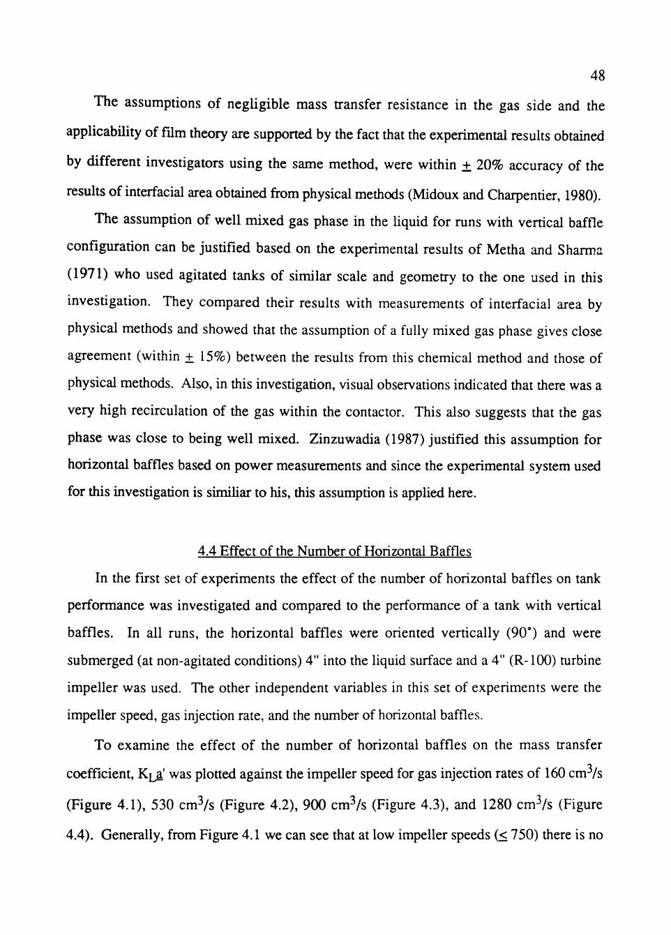
4.4 Effect of the Number of Horizontal Baffles

In the first set of experiments the effect of the number of horizontal baffles on tank

performance was investigated and compared to the performance of a tank with vertical

baffles. In all runs, the horizontal baffles were oriented vertically (90°) and were

submerged (at non-agitated conditions) 4" into the liquid surface and a 4" (R-lOO) mrbine

impeller was used. The other independent variables in this set of experiments were the

impeller speed, gas injection rate, and the number of horizontal baffles.

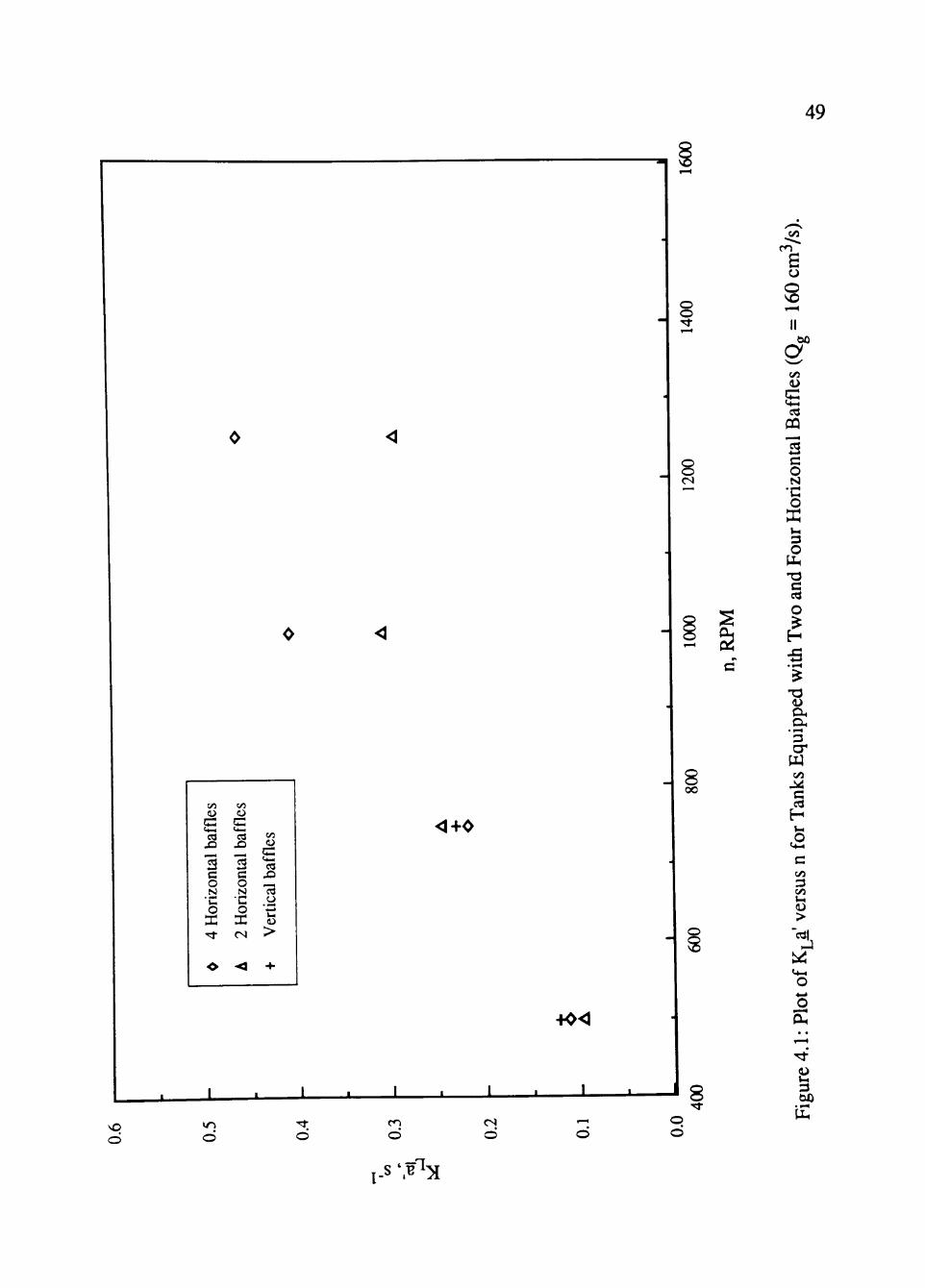
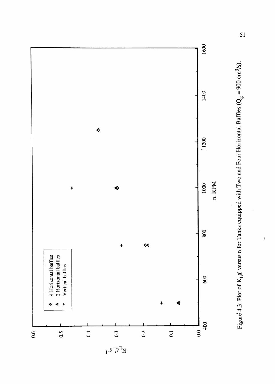
To examine the effect of the number of horizontal baffles on the mass transfer

coefficient, K]j! was plotted against the impeller speed for gas injection rates of 160 cm^/s

(Figure 4.1), 530 cm^/s (Figure 4.2), 900 cm^/s (Figure 4.3), and 1280 cm^/s (Figure

4.4). Generally, from Figure 4.1 we can see that at low impeller speeds (< 750) there is no

49

o o

o o

<y5

en

6 o O

NO

II bO

g D

CQ

"5 c o N •c o 3

o

c« (U

C ( M 03

X3

2 c o N •c o 3: '^

-o

oo o c u - l cd

X3

2 c o N •c o X cs

-<J

(/5 (U s (fl

X3

13 o

. — » <L)

>

+

<+0

00

+^<

o O o o o

-J 8 o c5

o

-S

u a, O H

'3 w C/3

c cd

H

W3

3 1>3 D >

O

o

V H

3

F1^ i-s '.B A:s

50

«>

o <

(73 4

^ ^ M

3 c o N k .

o X <N

<

Vi O

S X5

1

C3 O •5

>

+

<A

^0<

o

o o

8 fti

0 0

o o

CO

e o

O m

s (A

cd

"3 c o N

'C o 3 O

UH T3 C cd O

H -S

T3 <o cx

a, ' 3 cr W c H

<2 C/5

3 (Z) Vl

>

o

<N ^ '

3

vo o o o O

o c>

i-s '. ' :s

51

£ o o ON

so

2 (/) D

OQ

«s

2 c. o N

•c O

OH

3 O

T3 C CO

O

H

C« V3 O 0) P c: • ^ 'eg X ) X5

3 2 c c q o NJ N

•c -c O O

I X •rt CS

• '<l

V3 0)

C U - i

X)

« o

erti

>

+

o o

o o oo

<Xi

o o

o d o d

13 u ex

*3

D c/5

C cd

H

c/5 3 c« Vx

>

O

o

V l

3

p l ^ i-s '.H A:s

• 52

00 

+

+ 0<

\o

o o

(N

O o oo

o o

+ <

d d d d d o d

c/5

m £ o o oo II

60 a 0»5

CQ

c o N •c o Vl 3 O

PH -a c a O

T3 (U CL

' 3 a* W c/5

c

c/5 3 c« VH

>

o o

2^ 3

p l ^ l-s '.B y[

53

difference in KL^' for all baffle types, but at larger impeller speeds (> 1000) the tank

equipped with four horizontal baffles is better for mass transfer. Data on tanks with

vertical baffles is not available at these impeller speeds because the motor could not provide

enough power at this gas injection rate. By increasing the gas rate to 530 cm^/s (Figure

4.2) we see that there is no difference between the use of two and four horizontal baffles,

however, KLa' is greater for vertical baffles compared to horizontal baffles. This trend is

evident also at the higher gas rates of 900 cm^/s (Figure 4.3) and 1280 cm^/s (Figure 4.4).

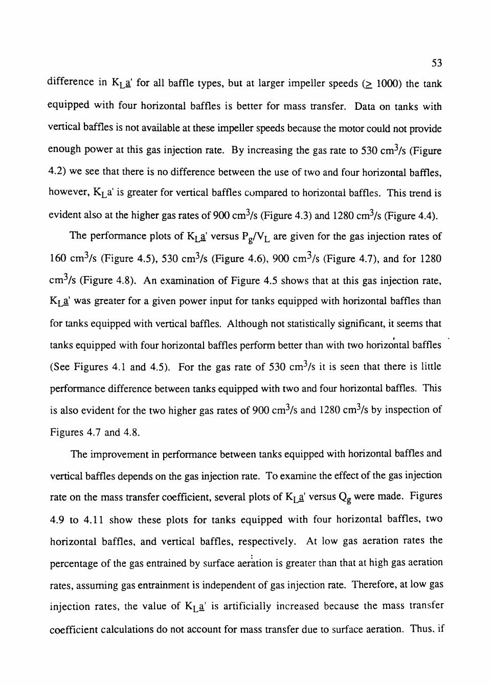
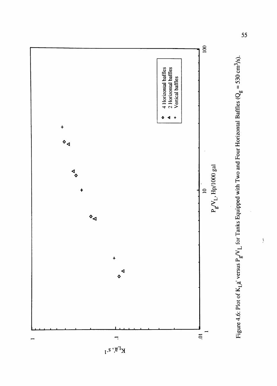
The performance plots of KLa' versus P^/VL are given for the gas injection rates of

160 cm^/s (Figure 4.5), 530 cm^/s (Figure 4.6), 900 cm^/s (Figure 4.7), and for 1280

cm^/s (Figure 4.8). An examination of Figiu-e 4.5 shows that at this gas injection rate,

KLa' was greater for a given power input for tanks equipped with horizontal baffles than

for tanks equipped with vertical baffles. Although not statistically significant, it seems that

tanks equipped with four horizontal baffles perform better than with two horizontal baffles

(See Figures 4.1 and 4.5). For the gas rate of 530 cm^/s it is seen that there is little

performance difference between tanks equipped with two and four horizontal baffles. This

is also evident for the two higher gas rates of 900 cm^/s and 1280 cm^/s by inspection of

Figures 4.7 and 4.8.

The improvement in performance between tanks equipped with horizontal baffles and

vertical baffles depends on tiie gas injection rate. To examine the effect of the gas injection

rate on the mass transfer coefficient, several plots of KL^' versus Qg were made. Figures

4.9 to 4.11 show these plots for tanks equipped with four horizontal baffles, two

horizontal baffles, and vertical baffles, respectively. At low gas aeration rates the

percentage of the gas entrained by surface aeration is greater than that at high gas aeration

rates, assuming gas entrainment is independent of gas injection rate. Therefore, at low gas

injection rates, the value of KLa' is artificially increased because the mass transfer

coefficient calculations do not account for mass transfer due to surface aeration. Thus, if

54

o<

Vi O

C U-r

talb

a

c o N UH

O X -rt

•

Vi ii

G Vw

talb

a

c o •c O X cs

<

affl

es

X) 13 o

ert

>

+

50

- O C-

> "^"50

c/5 CO

£ o

II bO g

c/5

D S PQ

13 c o N

•c o a:

V H

3 O •o C cd O

-a D O H

a, '3 cr W

c/5

c H

• • • • • ' V . I I I .J I I

CL, c/5

3 VH

>

O

in '^' <u VH

3 &0

t-s '.B'^:^

55

1 1 i

+

o<

< 0

+

• • • •

* <

+

< 0

* • • • • • •

baff

les

baff

les

les

4 H

oriz

onta

l 2

Hor

izon

tal

Ver

tical

baf

f

^ < *

•

•

•

•

'

—T

—•

• '

' •

' '

C3

O o o

- O

cu

c«

£ o o

CO >n

bO

s s OQ

13 c o •c o

V H

3 O

PU T3 C c« O

a> ex ex 3

w c/5

c cd

H VH

CU c/5

3 c/5 VH

(U >

o o

V H

3

p l . I-S '.B ^:^

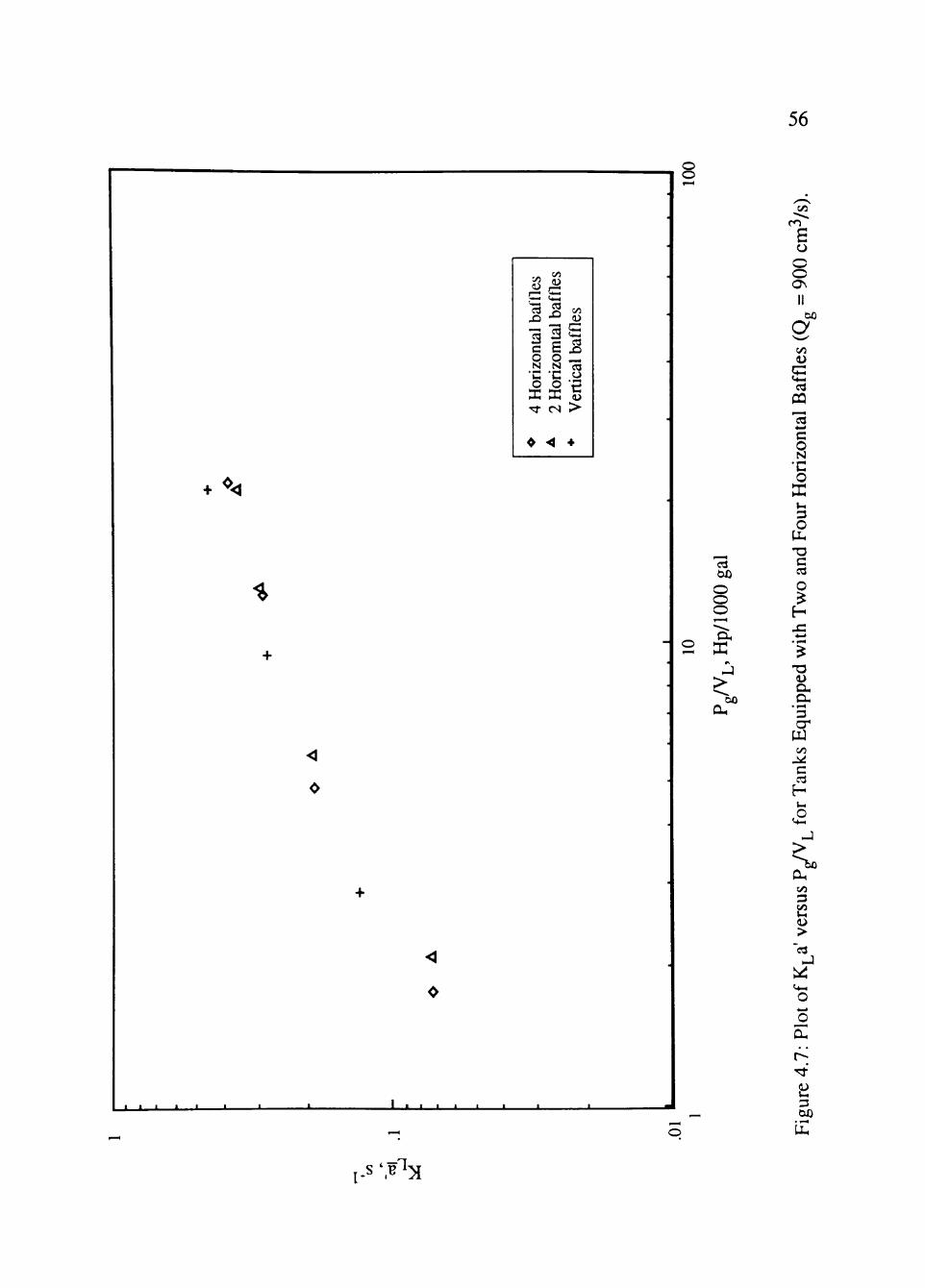
o o

56

*"><

%

<

0

Vi O r -

bal

ntal

o N U l

r/1

( M C3

3 s o N •c

o o X X T j -

•

cs

-4

c/5

baff

l

1 ,

CQ O

erti

>

4

c3

O o o " ^ X

DO

!/5

CO

£ o o ON

bO

g on

£ CQ

'B c o N

•c o PC

VH

3 O

PU T D G cd O

 'a

J J ^ C 4 - 1

o _o CU

3 (30

• £

p l . i-s '.B :s

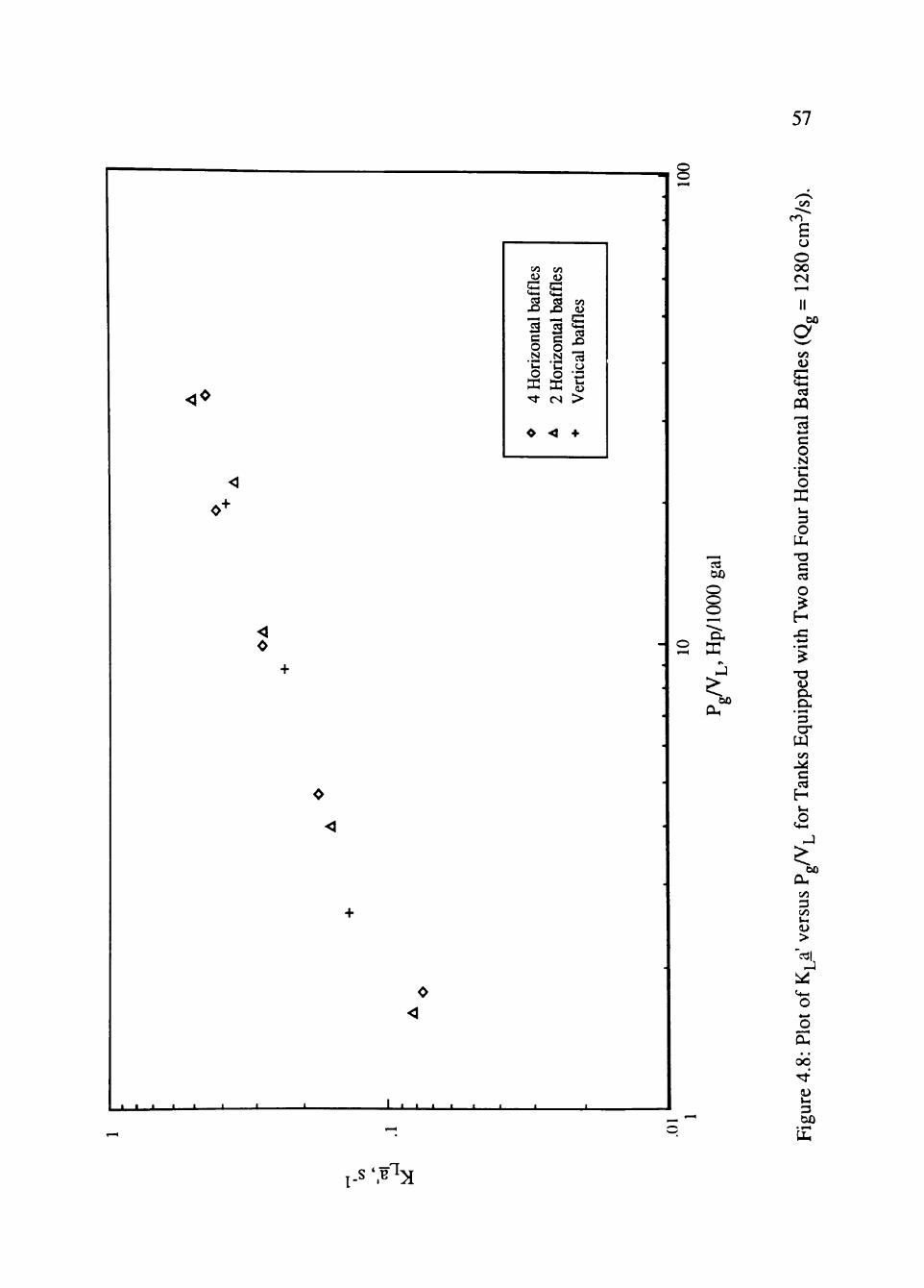
o o

57

<o

Vi 

+

c/5

£ o oo <N

II bO

2 00

CQ

13 4—1 c o N

•c o X

< 0

o o o "a, X

3 O

-o c cd

O

•a ex ex

• l - H

3 cr W 00

C cd

H

^ bO

' ' ' I I I I V . • • ' • '

0 0

3 oo VH

>

« * H

o o

66

V H

3

p l . i-s '. :s

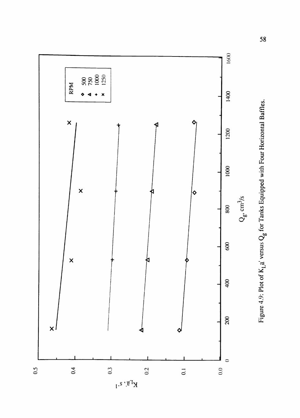
58

^ (X ai

8 »o

•

o </-i t^

<

o 8 +

^

CS

X

o

o o

o o cs

o o 00

00

£ CJ

bO

o

o o

cs

oo

u « H - |

CO

CQ

'2 c o Si

'C o X

V H

3 O

PU

T3 O ex ex

• ^-4

3 cr

W 00

c H

VH a bo

o 3 00 VH

>

« 4 - l

O

o

3

in

o o O <N O

i-s ' i ^ ' ^ : ^

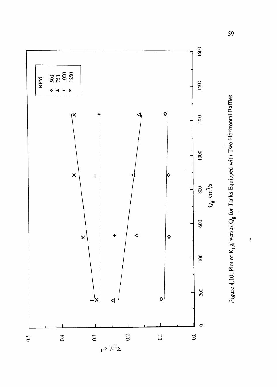
59

CU Oi

8 >o

•

o r-

<

000

^^

+

250

'—'

X

o o cs

c/5

£ OQ

13 4—> c o N

•c • o X o

o o oo £

o bO

D CX CX 3

W 00

M C

H

VO

o o

bO

o> Vi 3 Vi V H u >

<4- l

O

OH

o o cs 3 60

d CD cn d

cs d

o d

p l . i-s '.B :s

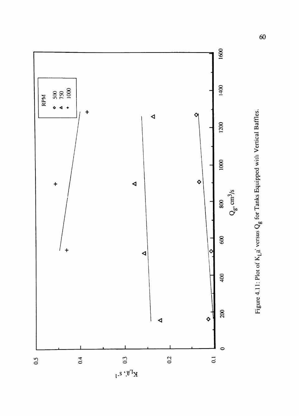
60

(X

Q ^ 'R o m o i n r~~ —'

^ < *

cs

c/5

£ C3

CQ 13

VH

>

oo

en

£ bO a

-a ex a, '3 a* W 00

C ca

H

VO

bO a 3 Vi

VH

>

o o

o o

cs

VH

3 60

in

d d d cs d

f-S '.^^M

61

surface aeration caused an increase in K^j! at low gas injection rates, the slopes of tiie lines

in Figures 4.9 to 4.11 would be negative. A two-variable statistical t-test was used to

determine if the slopes were distinguishable from zero at a 95% confidence level. Due to

the relatively large amount of scatter in tiie data this test indicated that for all three baffle

types the slopes were indistinguishable from zero. Thus, the dependence of KL^' on Qg is

not changed by tiie baffle type.

If surface aeration were the cause for the improvement in KLa' for four horizontal

baffles as found by Zinzuwadia (1987), the amount of gas in tiie dispersion will be greater

than for two horizontal baffles at the same conditions. This may be determined by plotting

the void fraction against the impeller speed for each baffle orientation. Figures 4.12 to

4.15 show these plots for gas injection rates of 160 cm^/s, 530 cm^/s, 900 cm^/s, and

1280 cm^/s, respectively. An examination of Figure 4.12 suggests that at the lowest gas

rate the void fraction for tanks equipped with four horizontal baffles is greater than that for

tanks equipped with two horizontal baffles. Thus, when four horizontal baffles are used

the entrainment of gas is greater than when only two were used. This suggests that surface

aeration is enhanced by the use of four horizontal baffles more than with two horizontal

baffles (See Figure 4.5). One would expect that four horizontal baffles at the liquid surface

would induce twice as much gas into the dispersion due to surface aeration (See Figure

4.12). Such would be the case if by the addition of two more baffles the flow patterns at

the surface were not changed. However, when two more baffles are added to the tank, the

local velocities near the surface are reduced, thus reducing the turbulence and inhibiting

surface aeration.

Also, the void fraction for tanks equipped with horizontal baffles is greater than for

tanks equipped with vertical baffles. Thus, the performance of tanks equipped with

horizontal baffles is better than with vertical baffles (See Figure 4.5).

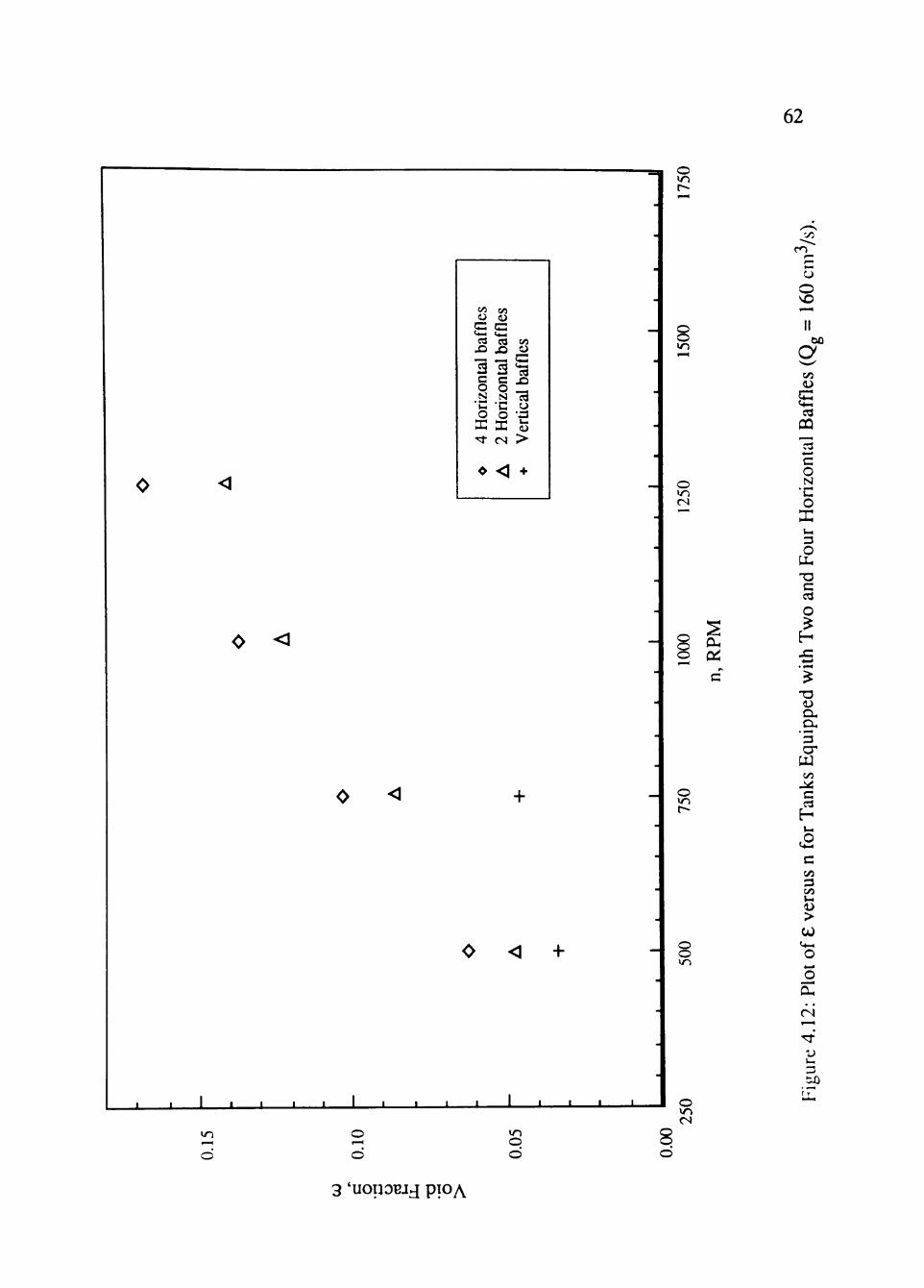
62

00 

+

o »n

o o m

o in

o 0

o >n

o o in

I • I L O vn cs

in

d m o

'^5

cn r— rH

o O vO

II bO s

oo

£ OQ

c

o N

•c o X

VH

3

o c CO O

XJ CO

Vt-H

O

CU

CN

k.

60

3 'uonom j PPA

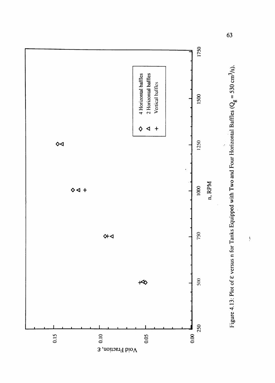
63

00 Hi

G • ^ X5

tal

c o N k.

o X ^

0

Vi 

+

0 <

0 < +

<H-<

-lO

o m

o o m

m (N

8 2

O m

o m (N

d m O

c/5 cn

£ o m

bo s oo

£ C3

CQ

c o N •c o

VH

3 O

-o c o

T3 ex & '3

W c/5

c cd

H

00 3 oo VH

>

W

O

o

^ ' D V H

3 60

3 'uotjOBij pioyv

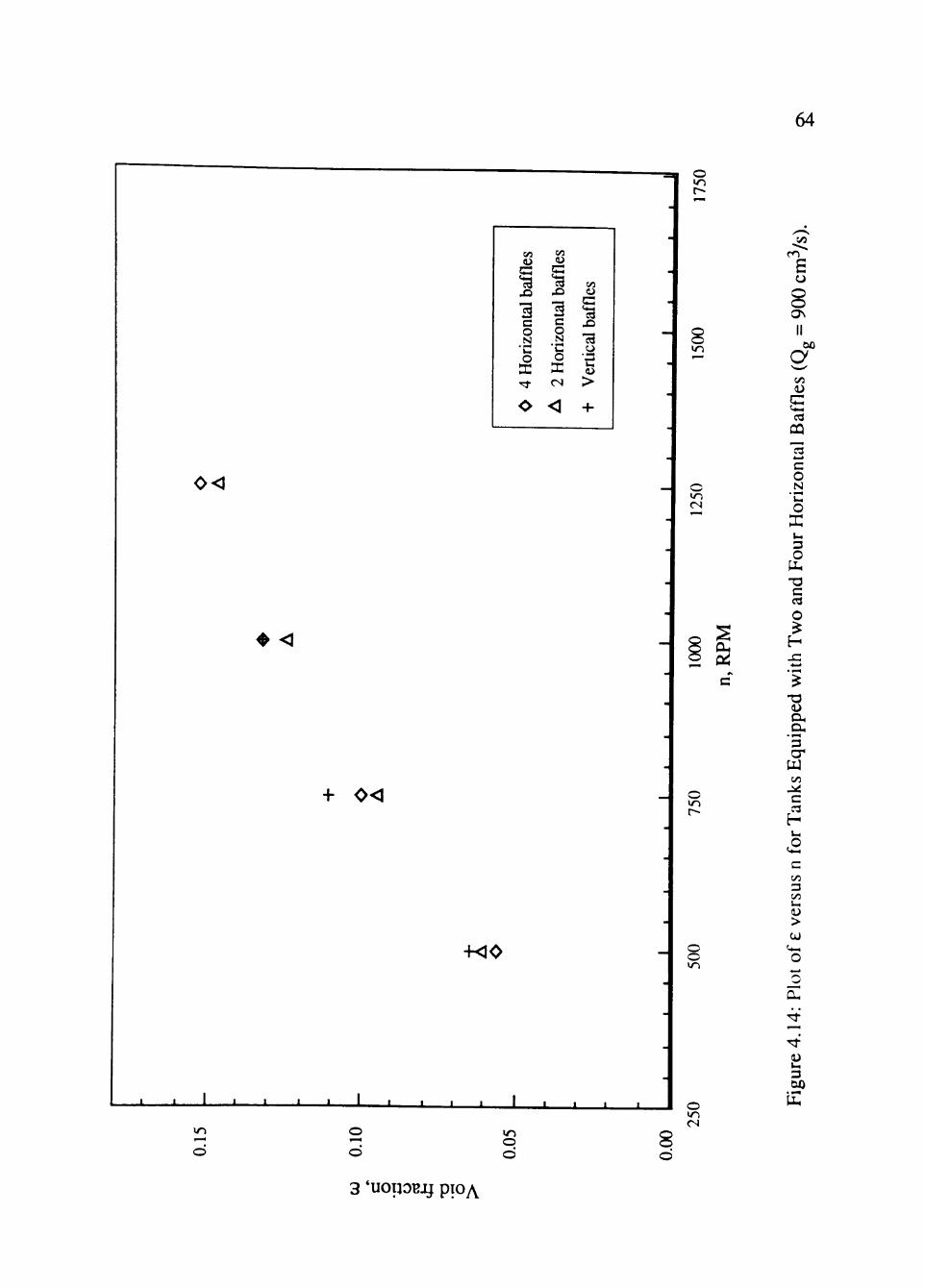
64

0 <

• <J

+ 0<1

CO (U c: 1^ Xl

tal

c o N kn

o X ^

o

Vi ii s 13 X5

3 c o N • c o X

(N

<

CO « s

X)

13 o • 3 Ui

0 >

+

-H30

o >n

m

m cs

o vn

o o i n

I I 1 I • •

d o d

m o d

o m cs

c/5

£

ON

bo

o Vi D

£ 03

CQ "2 c o

'u O 3:

VH

3 O tu -a c c3

O

(U O H CU 3 cr w 00

c r3

H VH

.0

00 3 c/)

VH

>

o

VH

3 60

3 'uopoBj^ plOy^

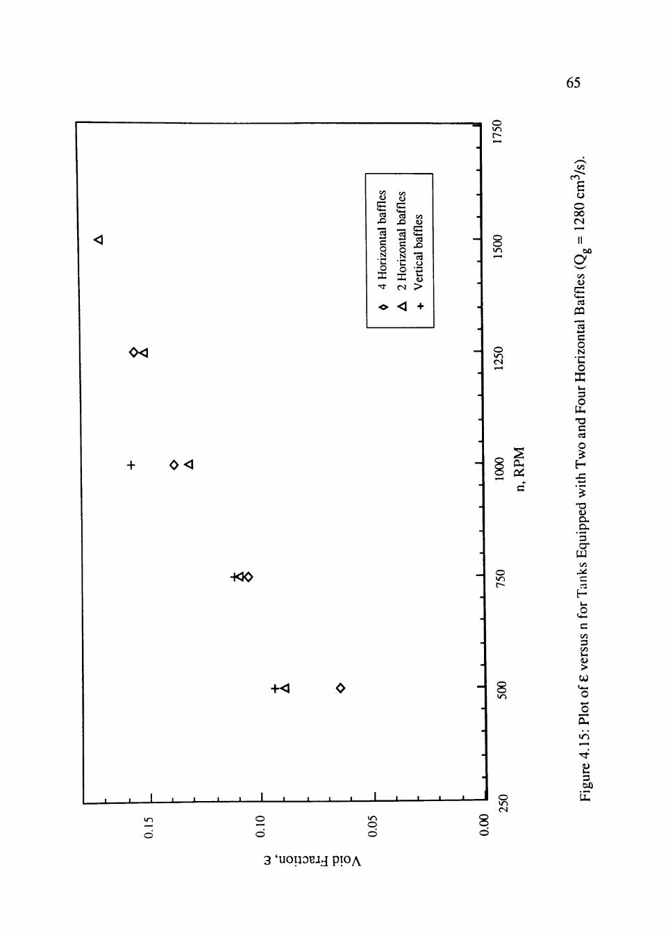
65

<

0<

S? 00 

o < +

_

-

^

—

•

-

-

o >n

0 <

4<0

•K l

o o m

O m cs

ii

o <n

m

J L O i n cs

m

d o d

i n O

c/5

m

£ u

O 00

bO

2 oo (O

< ^ C3

OQ

c O N

•c o X

VH

3 O

PU TD C cd O

D-

' 3 cr W 00

00 3 00 VH

>

(4-1

o o

vri

' ^

£i 3 60

3 'UOUDBJj pIOA

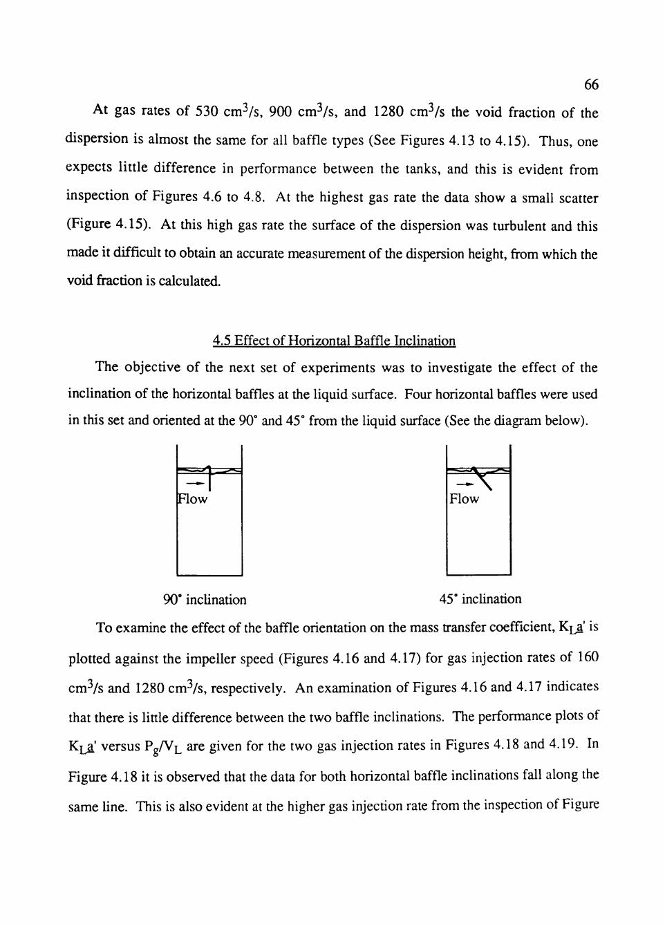
66

At gas rates of 530 cm^/s, 900 cm^/s, and 1280 cm^s the void fraction of the

dispersion is almost the same for all baffle types (See Figures 4.13 to 4.15). Thus, one

expects little difference in performance between the tanks, and this is evident from

inspection of Figures 4.6 to 4.8. At the highest gas rate the data show a small scatter

(Figure 4.15). At this high gas rate the surface of the dispersion was turbulent and this

made it difficult to obtain an accurate measurement of the dispersion height, from which the

void fraction is calculated.

4.5 Effect of Horizontal Baffle Inclination

The objective of the next set of experiments was to investigate the effect of the

inclination of the horizontal baffles at the liquid surface. Four horizontal baffles were used

in this set and oriented at the 90° and 45° from the liquid surface (See the diagram below).

90° inclination 45° inclination

To examine the effect of the baffle orientation on the mass transfer coefficient, K^a' is

plotted against the impeller speed (Figures 4.16 and 4.17) for gas injection rates of 160

cm- /s and 1280 cm^/s, respectively. An examination of Figures 4.16 and 4.17 indicates

that there is little difference between the two baffle inclinations. The performance plots of

KL^' versus PgA^L ^ ^ given for the two gas injection rates in Figures 4.18 and 4.19. In

Figure 4.18 it is observed that the data for both horizontal baffle inclinations fall along the

same line. This is also evident at tiie higher gas injection rate from the inspection of Figure

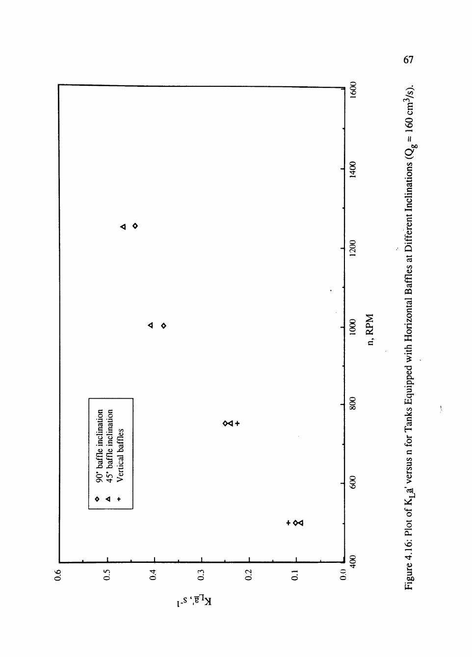
67

< 0

< •

c c o o •a -a C3 Ctl

c c CJ o

c c 'w^ '^m

(U (U

"c3t3 X5 X)

d tn o\ Tt-

• <

a> C C en

X>

cal

Ver

+

0< +

+ •<

o o

o o cs

o o 00

^

d i n

d d d cs d

t-s \^^:>i

Vi

m

£ CJ

o VO II

bo

g c/5 c o

•1.H

a c

. | . H

c c VH

cd 00

£ cd

CQ

«-• c o N

•c O

73 (U ex ex 3

W c/5

c H

VH

,o

OO 3 c/5 VH

>

o

'^'

VH 3 60

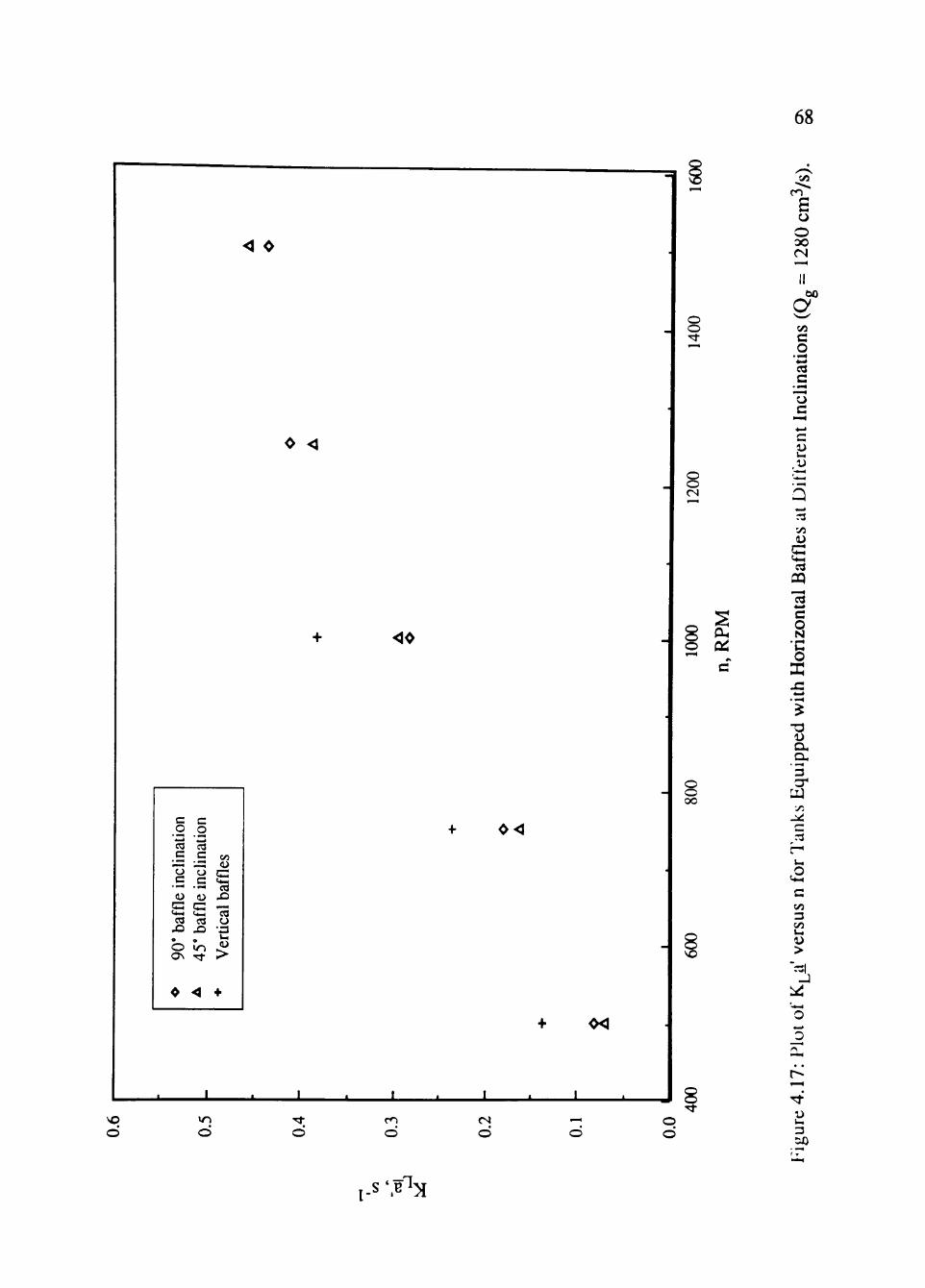
68

< 0

oo m

£ o

O

O O

bo

s Vi C o ^^ a c

"o c

0 <

«>

c o eg

lin

CJ c 

+

• <

•<

o o cs

si o 0

o o oo

VO

d d d en

d cs d

o d

c Si

r3 y5

£ C3

CQ

c o N •c o

T3 U ex a, 3

a Vi 3 00 VH

1) >

-J

"o 3 a-

D kn 3 50

l- s '.¥^ :s

69

c ^mi

a c

w ^

c —•

o c c3

Xi

C C3N

•

C

o • 3 CO c ^^ u c *" o c •^ x> • m • t

<

Vi a> s CQ . A

13

•5 o >

+

c/5 m

£ CJ

O VO

II bo o

C o

.<-H CO

c . 1 .H

c c Si

c/5 (U

£ <+H

PQ "^ c o N

•c o X

<rt T3 ex ex 3

W c/5

c c«

V H

.O

• < I—I

J L. ' • •

00 3 00 V H

>

o o

CX5

V^^ i-s '.B :s

Si 3 60

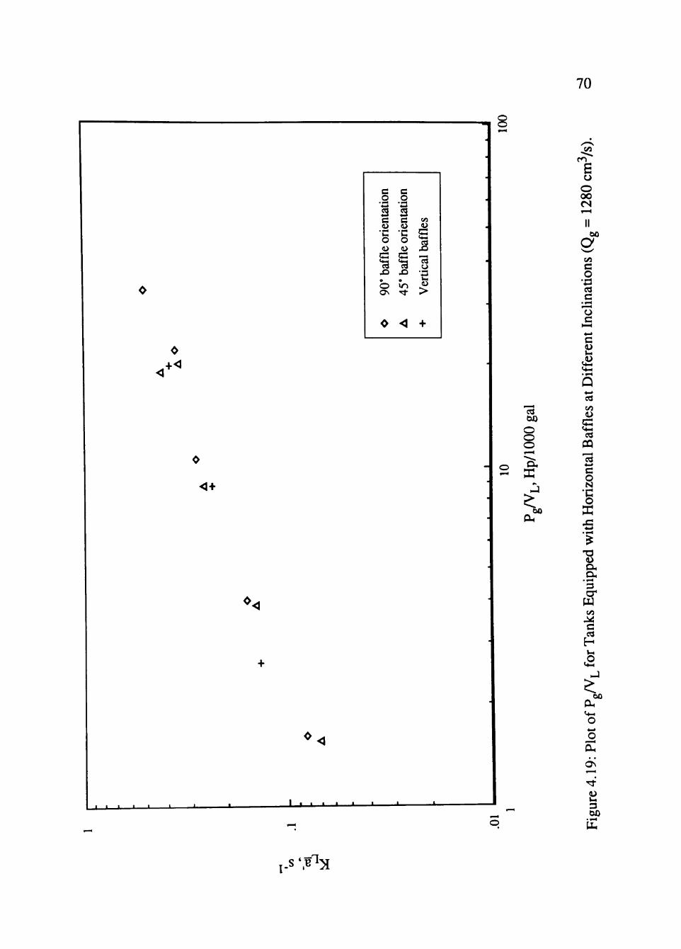
o o

70

c o ^ B a a kH

o c: 'H x> o

o as

0

c o •a a c (U

•c o a> G 13 x> «n -^

<

CO

u s .2 _ CU (J

•n

Ver

+

c/5 m

£ o 00 cs II

bo

s c/5 C o cd

c

c c Si

<+

cd 60

O o o

- O - X

5 .

cd 00

£ cd

CQ 73 c o N

•g X x: T3

-H

3 a' W oo C

bO

j _ i I I 1 1 - I «- ' • • • • '

O

O CU

2i 3 60

F l -i-s '.B :H

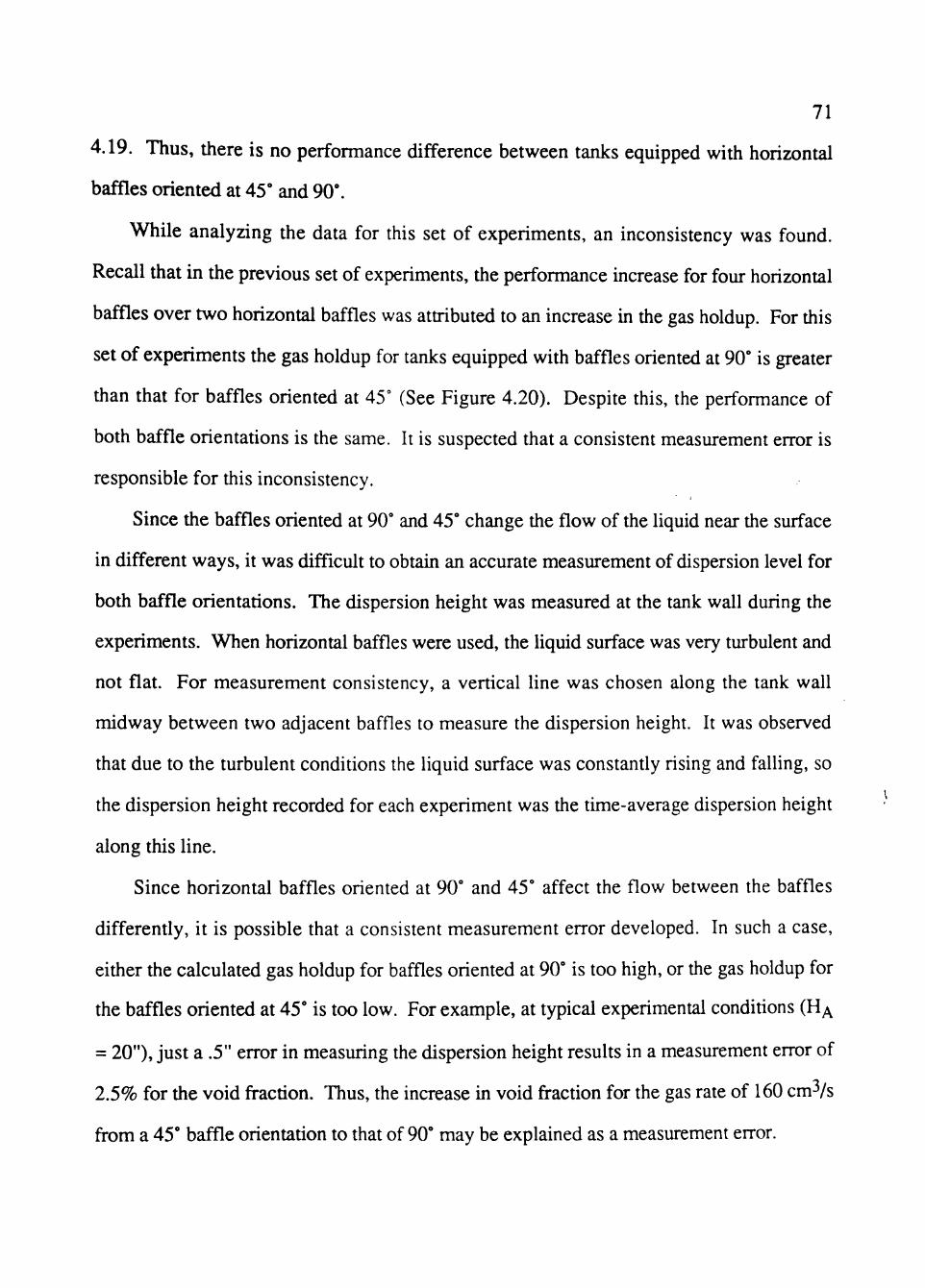
71

4.19. Thus, there is no performance difference between tanks equipped with horizontal

baffles oriented at 45° and 90°.

While analyzing the data for this set of experiments, an inconsistency was found.

Recall that in the previous set of experiments, the performance increase for four horizontal

baffles over two horizontal baffles was attributed to an increase in tiie gas holdup. For tiiis

set of experiments the gas holdup for tanks equipped with baffles oriented at 90° is greater

tiian that for baffles oriented at 45° (See Figure 4.20). Despite this, the performance of

both baffle orientations is the same. It is suspected that a consistent measurement error is

responsible for this inconsistency.

Since the baffles oriented at 90° and 45° change the flow of the liquid near the surface

in different ways, it was difficult to obtain an accurate measurement of dispersion level for

both baffle orientations. The dispersion height was measured at the tank wall during the

experiments. When horizontal baffles were used, the liquid surface was very turbulent and

not flat. For measurement consistency, a vertical line was chosen along the tank wall

midway between two adjacent baffles to measure the dispersion height. It was observed

that due to the turbulent conditions the liquid surface was constantiy rising and falling, so

the dispersion height recorded for each experiment was the time-average dispersion height

along this line.

Since horizontal baffles oriented at 90° and 45° affect the flow between the baffles

differentiy, it is possible that a consistent measurement error developed. In such a case,

eitiier the calculated gas holdup for baffles oriented at 90° is too high, or tiie gas holdup for

the baffles oriented at 45° is too low. For example, at typical experimental conditions (Hy

= 20"), just a .5" error in measuring the dispersion height results in a measurement error of

2.5% for the void fraction. Thus, the increase in void fraction for the gas rate of 160 cm^/s

from a 45° baffle orientation to that of 90° may be explained as a measurement error.

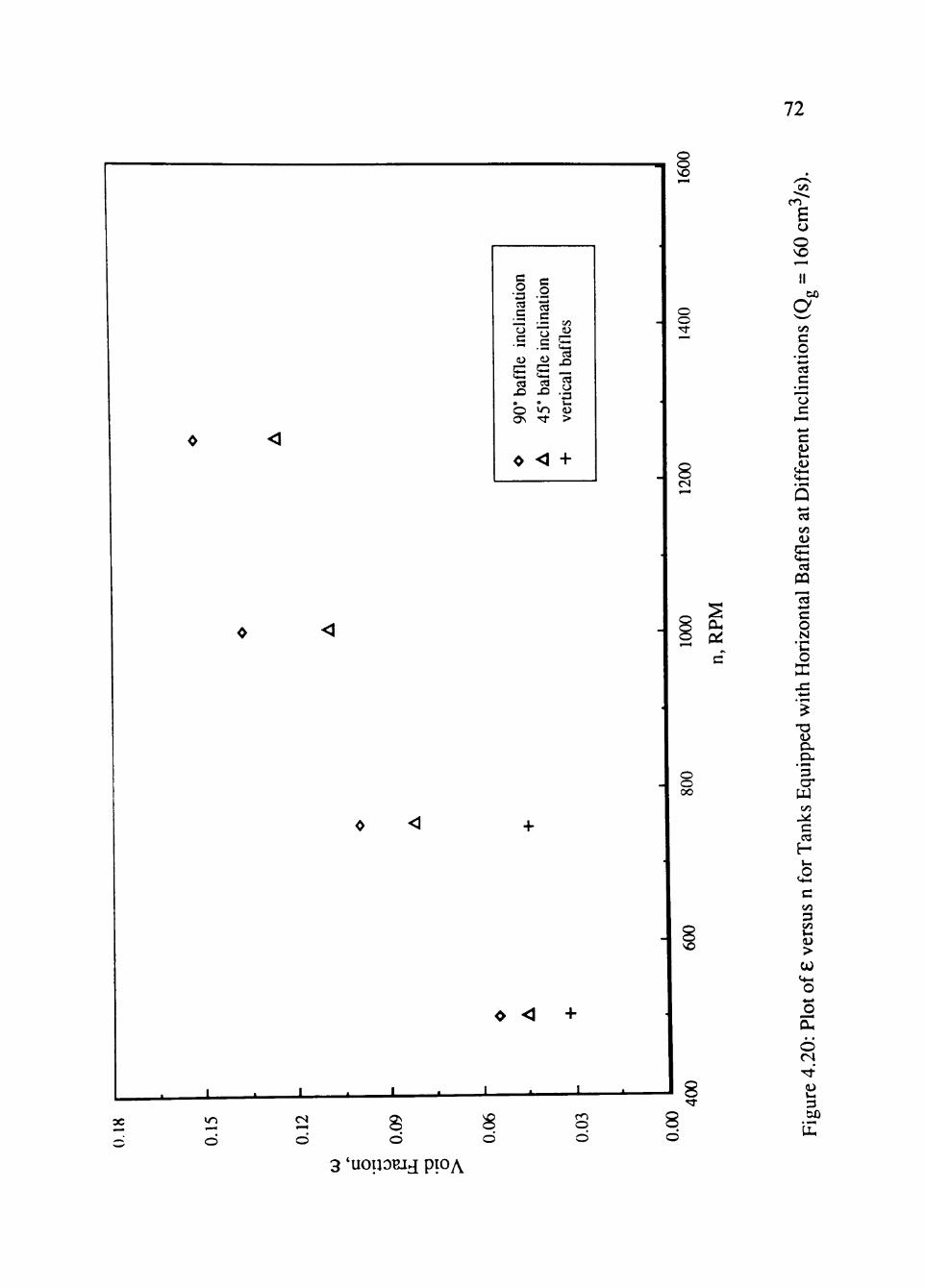
72

tion

ina

o c

<o C C cs Xi o

o OS

•

ion

nat

incl

i>

c ( « H eg

X) o

»n Tf

<

Vi U

Xi

tical

kH

(O >

+

o o VO

o o

cs

2 ^

o o oo

O <

± ±

VO

»n

d cs

d 8 d

O

c/5

£ o O VO

bO

s Vi C o c3 c

• ^

73 c c Si

c/5

£ cd

PQ

's c o N

•c o X

-a D CX

'3 W 00

C

a

c/5 3 c/5 V H

>

o o

CU

o ^ '

(U V H

3 60

UH

3 'uouoBJj ppA

73

At higher gas rates this error did not appear. When the tank was gassed at high rates

the baffles were completely submerged. At this condition, the surface of the dispersion

was not as turbulent, so the dispersion height is measured more accurately. Thus, when

the void fraction is plotted against tiie impeller speed for this gas rate (Figure 4.21) there is

littie difference between the baffle configurations.

4.6 Comparison witii Results of Zinzuwadia (1987)

The results obtained in this investigation were not consistent with those of Zinzuwadia

(1987). The performance of the tank equipped with vertical baffles performed better than

the one used by Zmzuwadia. Also, the performance increase of horizontal baffles was not

as large as reported by Zinzuwadia. At this point it was decided to try to duplicate the

results of Zinzuwadia using this experimental system.

The operating conditions used by Zinzuwadia were different than those used in this

investigation; he operated his system at gas injection rates of 154 cm^/s, 368 cm^/s, and

681 cm^/s. The gas injection rate (1280 cm^/s) used in this investigation is larger than that

used by Zinzuwadia. The experimental system used in this investigation differed in the

design of the horizontal baffle assembly. His horizontal baffles were four 1" strips of

polyacrylic at the liquid surface whereas in this investigation the baffles were 4.125" in

height. Zinzuwadia reported dispersion heights that would submerge the horizontal baffles

in the liquid. Because of the larger baffles used in this investigation, it was observed that

little liquid flowed over the upper edge of the baffle.

Another difference between the two experimental systems was the design of the

sparger. The sparger used in this investigation was a 4" ring mounted 2" above the tank

base. Into this 16 holes (.0938") were drilled into the top of the ring. The sparger used in

his investigation was made from copper tubing bent to form a 5" diameter ring and

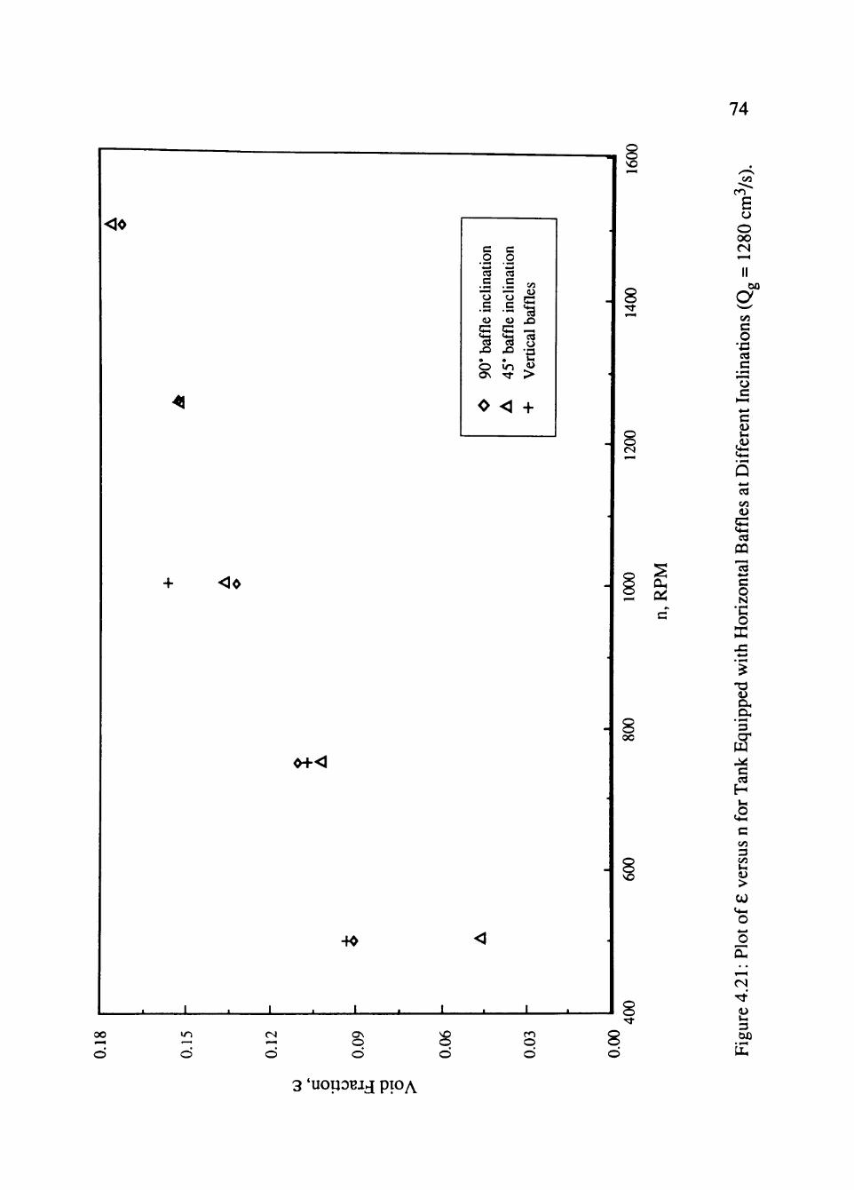
74

«>

^

«>

0+<

c c o o eg eg c c

c c (U a

G C •ta 13 X> Xi

o «n O N -TJ-

0 <

CO

u s X3

eg o •5 4> >

+

4^

o o VO

CS

« OH

2 Q

oo

c« m

£ o

bo

g c« C o

•a a c

73 c

oo

o m O

cs

o o o

VO

o o m O o

c VH

cd c«

£ cd

CQ

"5 c o N

•c o

-a

'3 cr W

H VH

.O

00 3 oo VH

>

O

CU

CN

<U VH

3 60

PU

3 'uopoBJj ptOA

82

2. Use a more acciu-ate method for determining the void fraction of the dispersion.

For example, recording several dispersion height measurements taken at different positions

around the tank perimeter may be a more accurate method to determine the void fraction.

3. Carry out experiments with a larger size contactor to develop scale-up relations.

4. Determine the effect of other geometric variables, such as, the submergence depth

of the horizontal baffles, impeller type and size, etc., on the performance of agitated tanks.

REFERENCES

Bruijn, W., Van't Reit, B., and Smith, J. M., Trans. Instn. Chem. Engrs., 52, 88 (1974).

Calderbank, P. H., Trans. Instn. Chem. Engrs., 36, 443 (1958).

Calderbank, P. H., Trans. Instn. Chem. Engrs. (London), 37, 173 (1959).

Chain, E. B., and Gualandi, G., R. C. sup. Sanit., 17, 5 (1954) (English edition), (Oxford: Blackwell).

Clark, M. W., and Vermeulen, T., Power Requirements for Mixing Gas-liquid Systems, UCRL-10996, Univ. of California, Berkeley (1963).

Cooper, C. M., Femstrom, G. A., and Miller, S. A., Ind. Engng. Chem., 36, 504 (1944).

Danckwerts, P. V., and Sharma, M. M., Br. Chem. Engnr., 15, 522 (1970).

Danckwerts, P. V., and Sharma, M. M., Chem Engnr., 44, 244 (1966).

Dickey, D. S., A. I. Ch. E. 72nd Annual Meeting, San Francisco, paper 116d (1979).

Dickey, D. S., and Fenic, J. G., Chem. Engng., 83, 139 (1976).

Dim, A., and Ponter, A. B., Chem. Engng. Sci., 26, 1301 (1971).

Eckenfelder, Jr., W. W., Principles of Water Quality Management, CBI Pub. Co. Boston (1980).

Elsworth R., Williams, V., and Harris-Smith, R., J. Appl. Chem., 1, 261 (1957).

Fuller, E. C , and Crist, R. H., J. Amer. Chem. Soc, 63, 1644 (1941).

Hassan, I. T. M., and Robinson, C. W., A. I. Ch. E. J., 23, 48 (1977).

Hatta, S., Technol. Repts., Tohoku Imp. University, 10, 119 (1932).

Hiegbie, R., Trans. A. I. Ch. E., 17, 365 (1935).

Holland, F. A., and Chapman, F. S., Liquid Mixing and Processing, Reinhold, New York (1966).

Joshi, J. B., Pandit, A. B., and Sharma, M. M., Chem. Engng. Sci., 37, 813 (1982).

Lewis, W. K., and Whitman, W., Ind. Engng. Chem., 16, 1215 (1924).

83

T • T. 8 4

Loiseau, B., Midoux, N., and Charpentier, J. C , A. I. Ch. E. J., 23, 931 (1977).

Loung, H. T., and Volesky, B., A. I. Ch. E. J., 25, 893 (1979).

Masheklar, R. A., and Soylu, M. A., Chem. Engng. Sci., 29, 1089 (1974).

Matsumara, M., Masunga, H., and Kobayashi, J., / . Ferm. Tech., 55, 388 (1977).

Metcalf and Eddy, Inc., Wastewater Engineering: Treatment/Disposal/Reuse, McGraw-Hill, New York (1979).

Metha, V. D., Ph. D. (Tech) Thesis, University of Bombay (1970).

Metha, V. D., and Sharma, M. M., Chem. Engng. Sci., 26, 461 (1971).

Michael, B. J., and Miller, S. A., A. 1. Ch. E. J., 8, 262 (1962).

Midoux, N., and Charpentier, J. C , BHRA 919, York 337-356, 3rd Conference on Mixing (1980).

Midoux, N., and Charpentier, J. C , Int. Chem. Engng., 24, 2 (1984).

Nagata, S., "Mixing," Wiley (1975).

Oldshue, J. Y., Fluid Mixing Technology, McGraw-Hill, New York (1983).

Perry, R. C , Green, D. W., and Maloney, J. O., Perry's Chemical Engineers Handbook, 6th Ed., McGraw-Hill, New York (1984).

Pharamond, J. C , Roustan, M., and Roques H., Chem. Engng. Sci., 30, 907 (1975).

Puchstein, A. F., Lloyd, T. C , and Conrad, A. G., Alternating Current Machines, 3rd ed., John Wiley and Sons, Inc., New York (1942).

Reid, R. C, and Sherwood, T. K., Properties of Gases and Liquids: Their Estimation and Correlation, McGraw-Hill, New York (1958).

Rushton, J. H., Costich, E. W., and Everet, H. J., Chem. Engng. Progr., 46, 395 (1950). i

Schultz, J. S., and Gaden, E. L., Industr. Engng. Chem., 48, 2209 (1956). t

Sherwood, T. K., and Pigford, R. L., Absorption and Extraction, McGraw-Hill, New '• •, York (1952).

Uhl, V. W., and Gray, J. B., Mixing, Theory and Practice, Academic Press, New York (1966).

Ulbrecht, J. J., and Patterson, G. K. Eds., Mixing of Liquids by Mechanical Agitation, Ch. 3, Gordon and Breach Science Publishers, New York, (1985).

Van Krevelen, D. W., and Hoftijzer, P. J., Rec. Trav. Chim., 67, 563 (1948).

85 Van't Reit, K., Boom, J. M., and Smith, J. M., Trans. Inst. Chem. Engrs., 54, 124

(1976).

Van't Reit, K., Bruijn, W., and Smith, J. M., Trans. Inst. Chem. Engrs., 52, 88 (1974a).

Van't Reit, K., and Smitii, J. M., Chem. Engng. Sci., 28, 1031 (1973).

Van't Reit, K., and Smitii, J. M., Chem. Engng. Sci., 28, 1093 (1974b).

Warmoeskerken, M. M. C. G., and Smith, J. M., Instn. Chem. Engrs. Symp. Series, 89, 59 (1984).

White, A. M., Brenner, E., Phillips, G. A., and Morrison, M. S., Trans. A.I.Ch.E., 30, 570 (1934).

Yung, C. N., Wang, C. W., and Chang, C. L., Can. J. Chem. Engng., 57, 672 (1979).

Zinzuwadia, H., M. S. Thesis, Texas Tech University (1987).

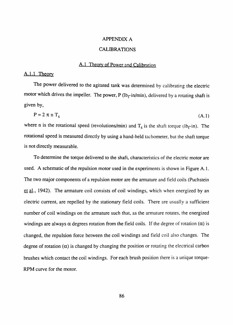
APPENDIX A

CALIBRATIONS

A.l Theory of Power and CaUbration

A. 1.1 Theory

The power delivered to the agitated tank was determined by calibrating the electric

motor which drives the impeUer. The power, P (Ibpin/min), delivered by a rotating shaft is

given by.

P = 2 7t n T s (A.l)

where n is the rotational speed (revolutions/min) and T is the shaft torque (Ibf-in). The

rotational speed is measured directly by using a hand-held tachometer, but the shaft torque

is not directly measurable.

To determine the torque delivered to the shaft, characteristics of the electric motor are

used. A schematic of the repulsion motor used in the experiments is shown in Figure A.l.

The two major components of a repulsion motor are the armature and field coils (Puchstein

et al., 1942). The armature coil consists of coil windings, which when energized by an

electric current, are repelled by the stationary field coils. There are usually a sufficient

number of coil windings on the armature such that, as the armature rotates, the energized

windings are always a degrees rotation from the field coils. If the degree of rotation (a) is

changed, the repulsion force between the coil windings and field coil also changes. The

degree of rotation (a) is changed by changing the position or rotating the electrical carbon

brushes which contact the coil windings. For each brush position there is a unique torque-

RPM curve for the motor.

86

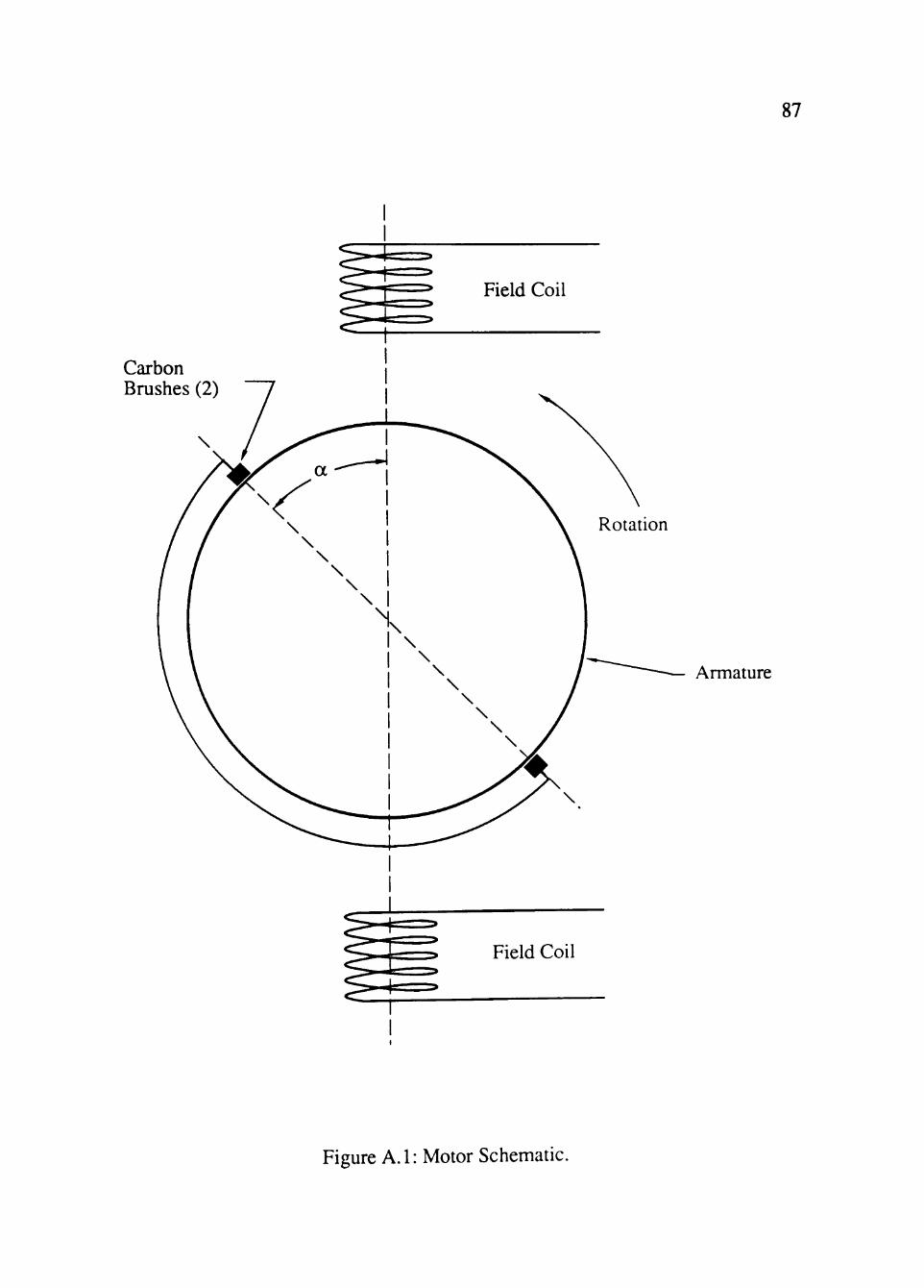
87

Carbon Brushes(2)

Armature

Figure A.l: Motor Schematic.

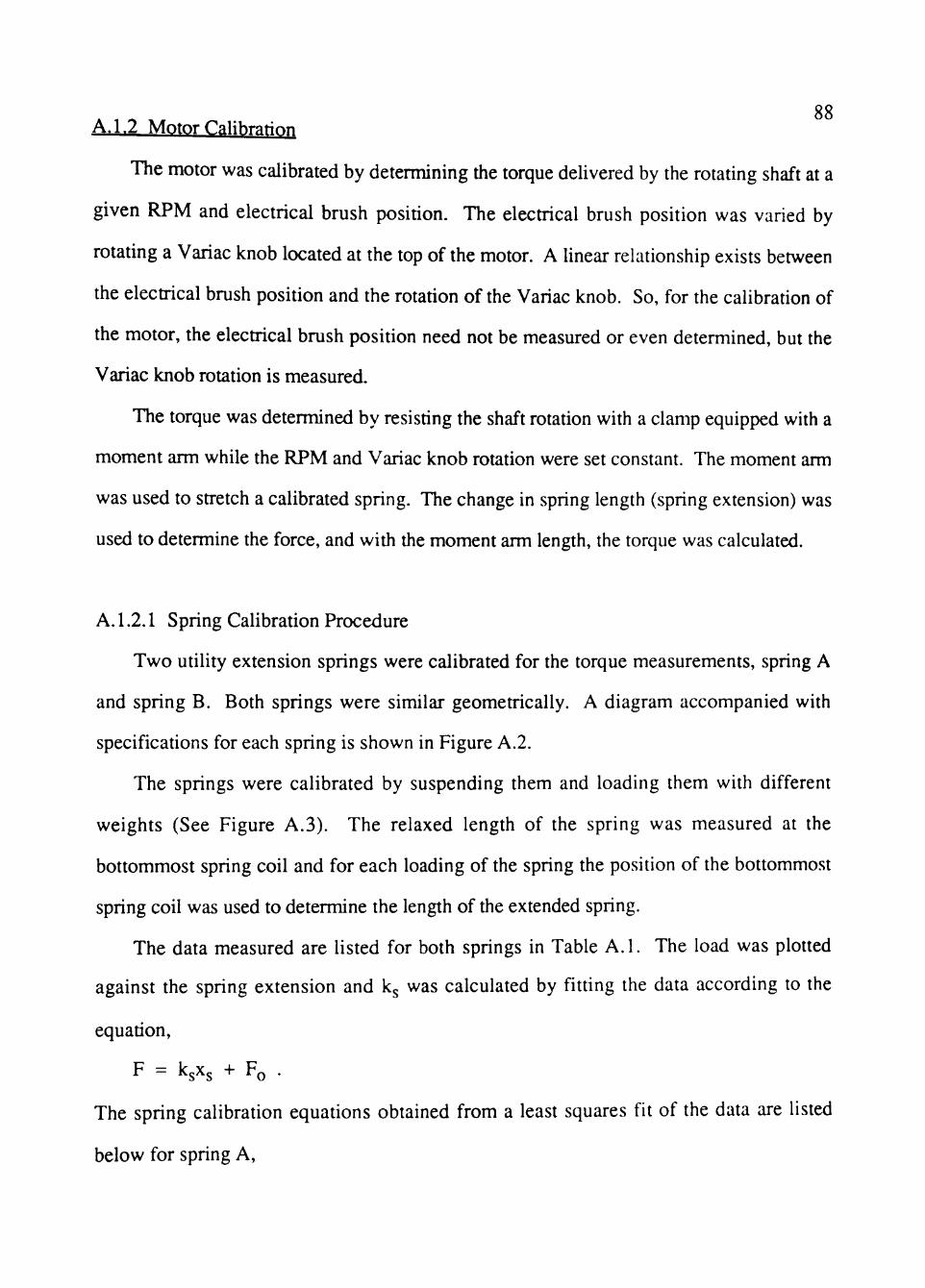
88 A. 1.2 Motor Cahhrntion

The motor was calibrated by determining tiie torque delivered by the rotating shaft at a

given RPM and electrical brush position. The electrical brush position was varied by

rotating a Variac knob located at the top of the motor. A Unear relationship exists between

the electrical brush position and the rotation of the Variac knob. So, for the calibration of

the motor, the electrical brush position need not be measured or even determined, but the

Variac knob rotation is measured.

The torque was determined by resisting the shaft rotation with a clamp equipped with a

moment arm while the RPM and Variac knob rotation were set constant. The moment arm

was used to stretch a calibrated spring. The change in spring length (spring extension) was

used to determine the force, and with the moment arm length, the torque was calculated.

A. 1.2.1 Spring Calibration Procedure

Two utility extension springs were calibrated for the torque measurements, spring A

and spring B. Both springs were similar geometrically. A diagram accompanied with

specifications for each spring is shown in Figure A.2.

The springs were calibrated by suspending them and loading them with different

weights (See Figure A.3). The relaxed length of the spring was measured at the

bottommost spring coil and for each loading of the spring the position of the bottommost

spring coil was used to determine the length of the extended spring.

The data measured are listed for both springs in Table A.l. The load was plotted

against the spring extension and kj was calculated by fitting the data according to the

equation,

r = l s s " ^o •

The spring calibration equations obtained from a least squares fit of the data are listed

below for spring A,

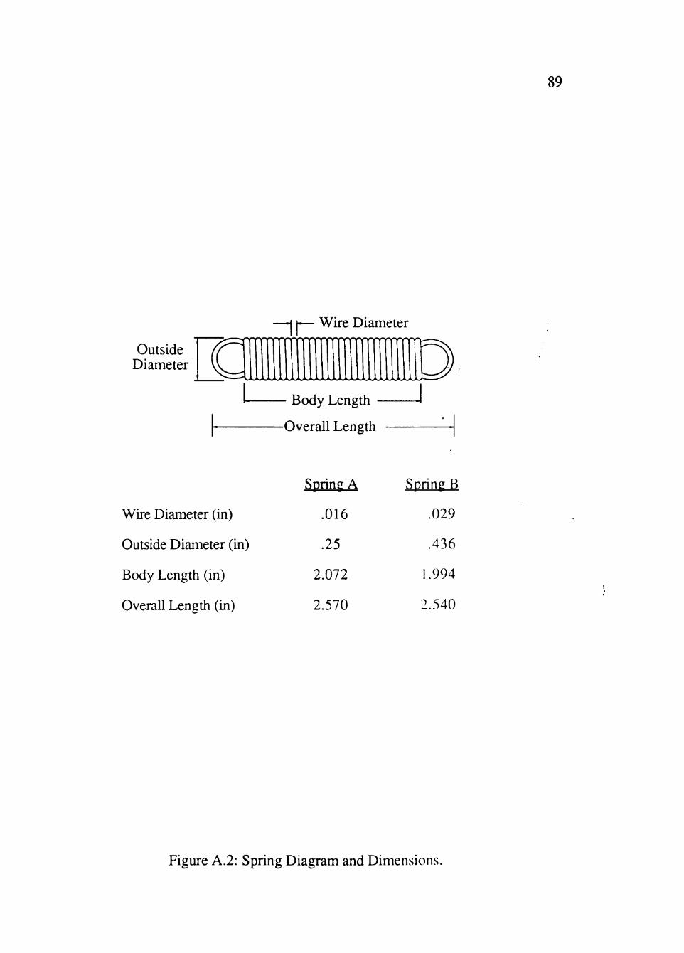
89

Outside Diameter

—I h— Wire Diameter

Body Length -

-Overall Length

Wire Diameter (in)

Outside Diameter (in)

Body Length (in)

Overall Length (in)

Spring A

.016

.25

2.072

2.570

Spring B

.029

.436

1.994

2.540

Figure A.2: Spring Diagram and Dimensions.

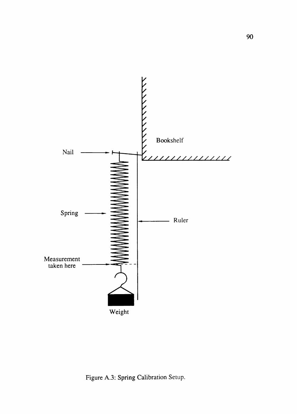
90

Nail

/ / / /

/ / / /

Bookshelf

Spring

Measurement taken here

\ y / / / / / / / / / / / / / / /

Ruler

Weight

Figure A.3: Spring Calibration Setup.

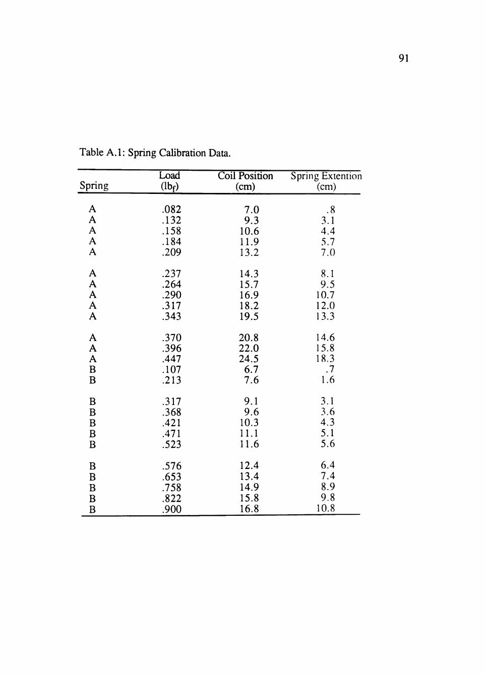
91

Table A.l: Spring CaUbration Data.

Spring

A A A A A

A A A A A

A A A B B

B B B B B

B B B B B

Load (Ibf)

.082

.132

.158

.184

.209

.237

.264

.290

.317

.343

.370

.396

.447

.107

.213

.317

.368

.421

.471

.523

.576

.653

.758

.822

.900

Coil Position (cm)

7.0 9.3

10.6 11.9 13.2

14.3 15.7 16.9 18.2 19.5

20.8 22.0 24.5 6.7 7.6

9.1 9.6

10.3 11.1 11.6

12.4 13.4 14.9 15.8 16.8

Spring Extention (cm)

.8 3.1 4.4 5.7 7.0

8.1 9.5

10.7 12.0 13.3

14.6 15.8 18.3

.7 1.6

3.1 3.6 4.3 5.1 5.6

6.4 7.4 8.9 9.8

10.8

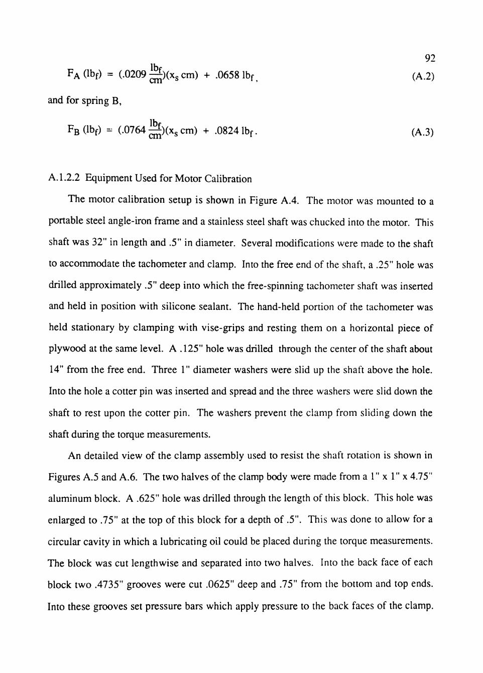
92

FA (Ibf) = (.0209 ^ ) ( x s cm) 4- .0658 Ibf, (A.2)

and for spring B,

FBdbf) - (.0764 ^ ) ( x s cm) + .0824 Ibf. (A.3)

A. 1.2.2 Equipment Used for Motor Calibration

The motor calibration setup is shown in Figure A.4. The motor was mounted to a

portable steel angle-iron frame and a stainless steel shaft was chucked into the motor. This

shaft was 32" in length and .5" in diameter. Several modifications were made to the shaft

to accommodate the tachometer and clamp. Into the free end of the shaft, a .25" hole was

drilled approximately .5" deep into which the free-spinning tachometer shaft was inserted

and held in position with silicone sealant. The hand-held portion of the tachometer was

held stationary by clamping with vise-grips and resting them on a horizontal piece of

plywood at the same level. A .125" hole was drilled through the center of the shaft about

14" from the free end. Three 1" diameter washers were slid up the shaft above the hole.

Into the hole a cotter pin was inserted and spread and the three washers were slid down the

shaft to rest upon the cotter pin. The washers prevent the clamp from sliding down the

shaft during the torque measurements.

An detailed view of the clamp assembly used to resist the shaft rotation is shown in

Figures A.5 and A.6. The two halves of the clamp body were made from a 1" x 1" x 4.75"

aluminum block. A .625" hole was drilled through the length of this block. This hole was

enlarged to .75" at the top of this block for a depth of .5". This was done to allow for a

circular cavity in which a lubricating oil could be placed during the torque measurements.

The block was cut lengthwise and separated into two halves. Into the back face of each

block two .4735" grooves were cut .0625" deep and .75" from the bottom and top ends.

Into these grooves set pressure bars which apply pressure to the back faces of the clamp.

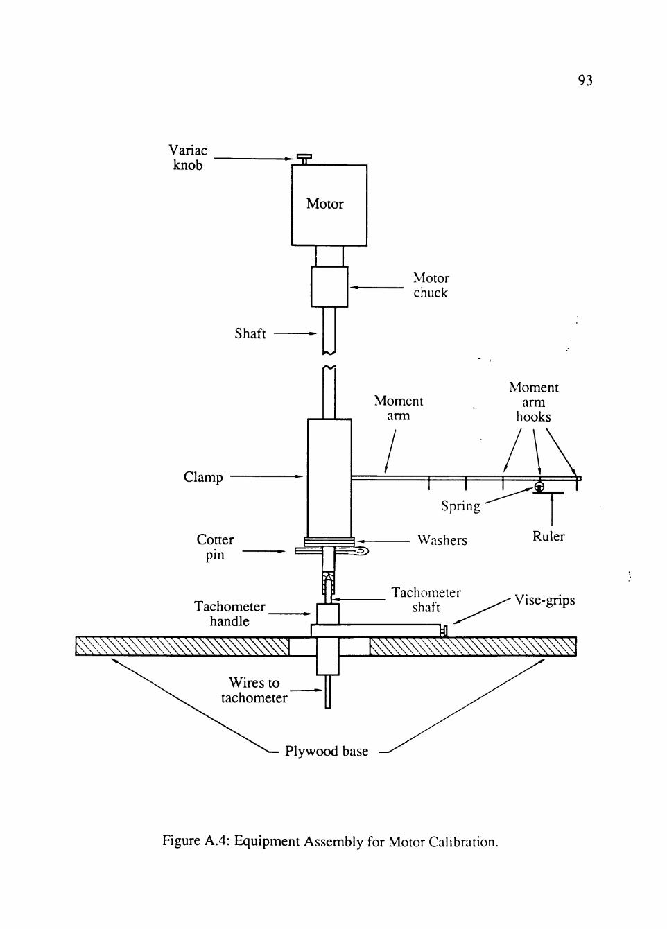
93

Variac knob

Clamp

Tachometer handle

Moment arm

k\\x\\\\\\\\\\\\\\\\\\m^

Motor chuck

Moment arm

hooks

I I I Spring

Washers

Tachometer shaft

Ruler

Vise-grips

fl ^ ^ ^ ^ ^ ^ ^

Wires to tachometer

Plywood base

Figure A.4: Equipment Assembly for Motor Calibration.

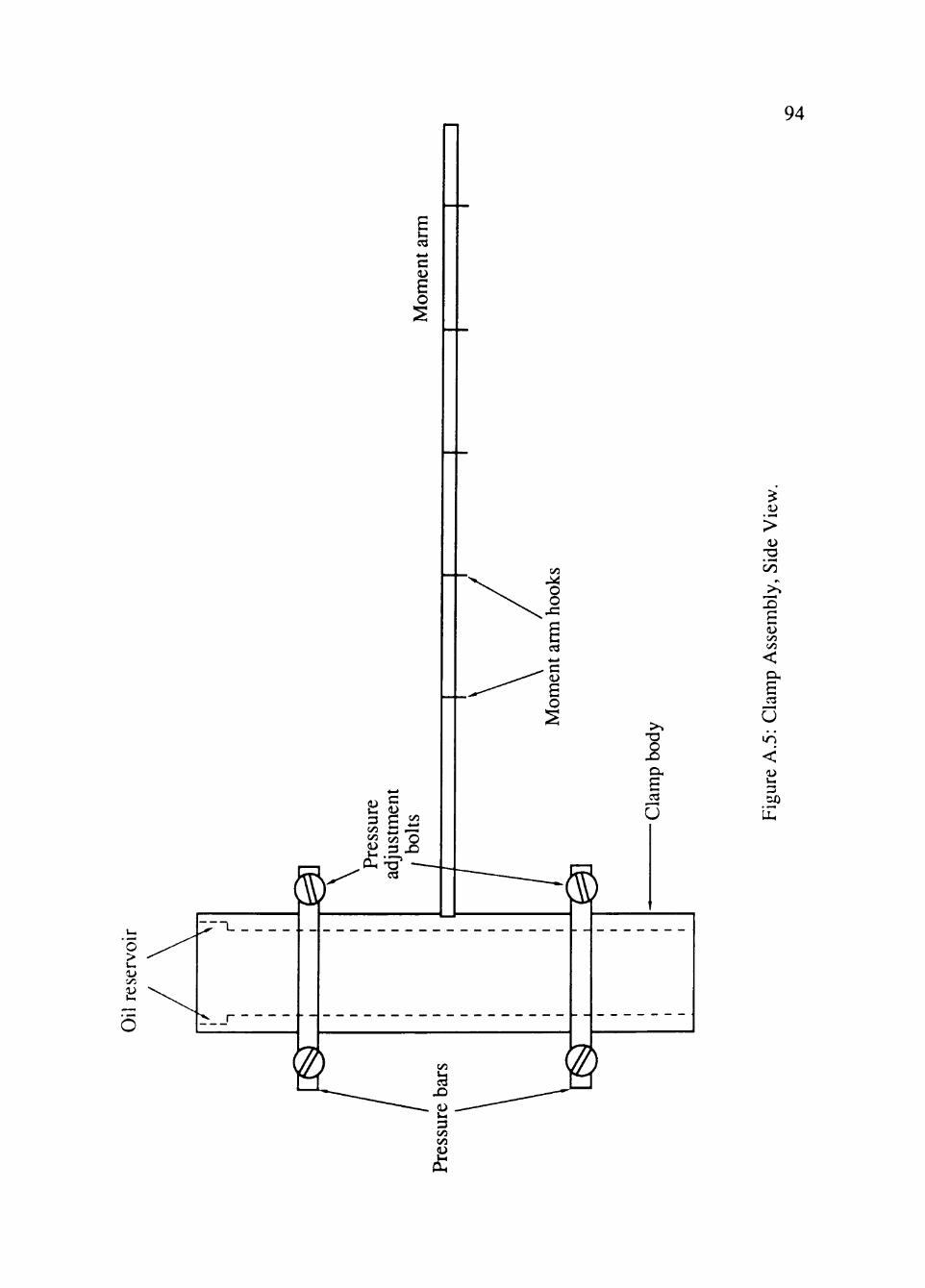
94

."2

IS £ Vi Vi

<

£ u

< •

OJ VH

3 60

3 C/3 C/5

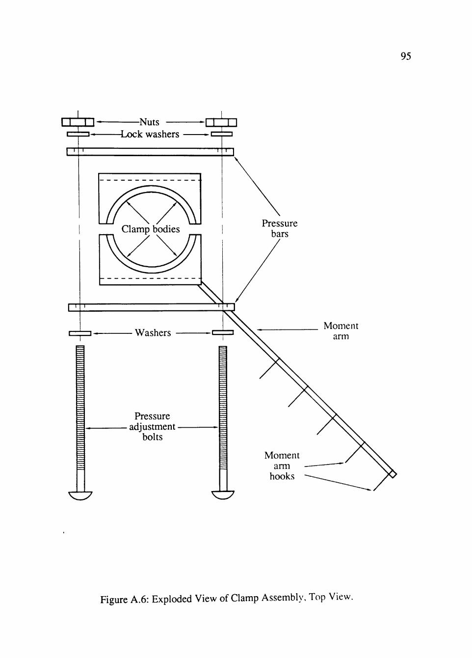
95

r r r n —Nuts -nzpn -Lock washers 1

Pressure bars

Moment arm

Figure A.6: Exploded View of Clamp Assembly, Top View.

96

The four bolts passing through the holes drilled through tiie pressure bars were used for

adjustment of the pressure to the shaft. Into the edge of one of the clamp bodies, a .125"

hole was drilled and threads tapped.

A .1875" brass rod of 12" length was used as the torque moment arm. Threads were

cut onto tiie end of this rod and the rod was screwed into the hole in the clamp body. Steel

hooks made from paperclips wcie soldered to the moment arm at distances of

4",6",8",10", and 12" from the clamp center. These hooks were provided for the

attachment of a spring end loop.

A strip of leather was used as a brake lining. The leather chosen was of medium

weight (.06" in thickness) and its dimensions were 4.5" x 3" (approx.). This strip of

leather was saturated with a light-weight machining oil for lubrication and to keep the

leather from drying out and burning during the torque measurements.

A. 1.2.3 Procedure for Motor Calibration

The torque measurements were obtained by the following procedure. With the motor

shut off the shaft assembly was inserted into the motor chuck and the chuck nut tightened.

A small amount of silicone sealant was applied to the free-spinning tachometer shaft and

this was insened into the hole drilled into the free end of the motor shaft. The silicone

sealant was allowed to cure for at least 12 hours before the motor was operated.

The leather strip was wrapped around the shaft in the direction of shaft rotation about

2" above the washers. The two halves of the clamp were placed around the leather strip.

The four pressure bars, bolts, washers, and nuts were then added. The bolts were hand

tightened so the clamp would not resist the rotation of tiie shaft. The clamp assembly and

leather were slid down the shaft until it rested upon the washers. The motor was then

turned on and was allowed to operate for 20 minutes at about 2000 RPM to allow the motor

to achieve a steady state operating temperature. The moment arm conveniently rotated and

97

hit the angle iron frame which kept the clamp assembly from rotating with the shaft. Care

was taken to enstu^ that the clamp offered no resistance to the rotation of the shaft. Oil was

periodically applied to keep tiie leather and shaft lubricated. After the motor had reached a

steady state operating temperature the variac knob was rotated to the selected position. A

spring was selected according to the magnitude of the torque anticipated. The layout of the

ruler, spring, clamp and moment arm is shown in Figure A.7. The moment arm hook was

selected according to the torque anticipated for the operating conditions of the motor. The

motor was slowed to 50 RPM less than the selected motor speed by tightening the bolts.

The rotational speed of the shaft gradually increased and when the proper RPM was

reached, the position on the ruler below the farthest spring coil was noted. The input

power was then noted from the wattmeter which was located within sight. Immediately,

the four pressure bolts were loosened so to offer no resistance to the shaft rotation.

A. 1.2.4 Motor Calibration Data and Chart

The data collected during the calibration of the motor are listed in Table A.2. A

calibration chart for the motor was made by plotting the torque versus the variac knob

rotation for different RPM. This chart was used during tiie experimental runs to determine

the shaft torque. This calibration chart is shown as Figure A.8.

A. 1.2.5 Sample Calculation

A sample calculation is given for the determination of the data presented in Table A.2.

The raw data recorded during a calibration is shown below.

Variac knob rotation 210°,

RPM 1500/min,

Spring coil position 18.8 cm.

Spring type A,

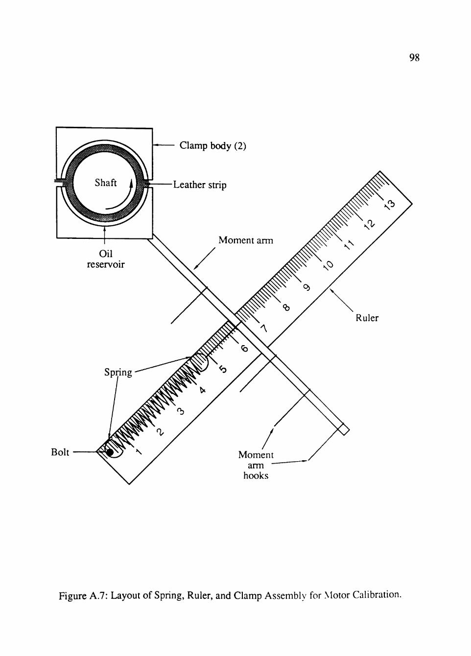
98

Oil reservoir

Clamp body (2)

Leather strip

Bolt Moment arm

hooks

Figure A.7: Layout of Spring, Ruler, and Clamp Assembly for Motor Calibration.

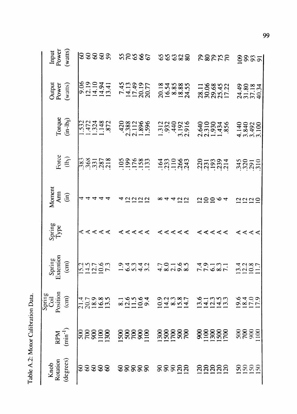
99

n

Q 3

o

U Ui

O

<

.a n

H

a. > c o ^ a.

6/)

v.

(U ,7v

§-^ V H I

O C

c

£ £ 1^

.3 a.

00

c 60 O

CL.B 00 X

Q O O O ON vC VO VO vO lO

»0 O >0 vO t^ lo r^ VO VO

»o w-i m <N o VC VO vO 00 00

ON O ON >0 C r^ CO r^ r~- r--

ON ON m -O ON ON ON

vO ON O -^ -^ O —< — ON rt ON ri Tt Tf CO

»0 m ON Ov r ' . ' . '^ .

t^ ' ' l^ O O -^ -^ <N <N

OO Tt lO OO »o ^ »0 OO OO lO O VC od oo Tt rs -^ —' <N

'—' NO oo »0 <N ^ P VO Tt CN od o ON >o r- <N en <N «N -^

ON O 00 Tf Tt OO —' c<-i ' —' r- d

CN CO en Tt

(N CN Tt OO CN

ro r- cN Tt r--lo - m ^ oo

O oo CN VO VO CN 00 ON ON Tt CO OO >o • • • • • CN (N -^ '—

(N rN O CN VO —' ro Tf ON T- ro ON Tf <—1 Ov

' ro oi

O O O ^ VO Tf r-H CO ro m VO ro Ov "^ OO • • • • •

<N <S —I 1—I

O O (N O '' ON O —' oo Tf ^ •«f ro ro ro

CO 3c -^ r>. oo 3C vo ro oo ^ ro CO CO (N rN

lo Ov VO oo ro O Ov r- »o ro

•^ ro o VO ro VO ro —' VO Tf -^ <N — fN (N

O ^ ro ON Tf CN ro ON ro <N CN <—! <N <N

lO o - o "" <N OS -^ ro ro CN CO

' ^ ' ^ T f T f T f T f < N ( N ( N < N O O T f r f r ^ c N i ( N O O V O T f CNCNCNO

< < < < < < < < < < < < < < < < < < < < < < < <

CJ

— O u o .3; 3

s: .£ a: £

c X i o

c/5

VH

o j i o r ^ v c r o O N T f c o T f c s

»r i CN O r- ^ vd uS Tf CO

r - o — VO u-i

Tf oo cs ON od Tf ON ^^ r o —1 r- r- VO od r-

Tf CN oo r -CO <N o —'

Tf r-- ON oo »o —* o od vd CO (N 0< —I ^ '-H

'—I VO l o vq Tf

od CN '—< O Ov

Ov CN r o oo r^ O Tf od »0 Tf

vq --< r o >o CO CO Tf CN Tf CO

vq Tf O ON

ON od r^ r-

lO r^ ON ^^ CO uo i n t ^ ON "-^ CO »o r^ «r> r^ ON '—' r o »o r^ ^^ 55 ^^ ^5 LO r - —

_; o o o o vO vO vO vO VO o oooo

^ ON ON Ov ON

o o o o o ON ON ON CN CN

ooooo CN CN CN CN CN

lO LO t o LO

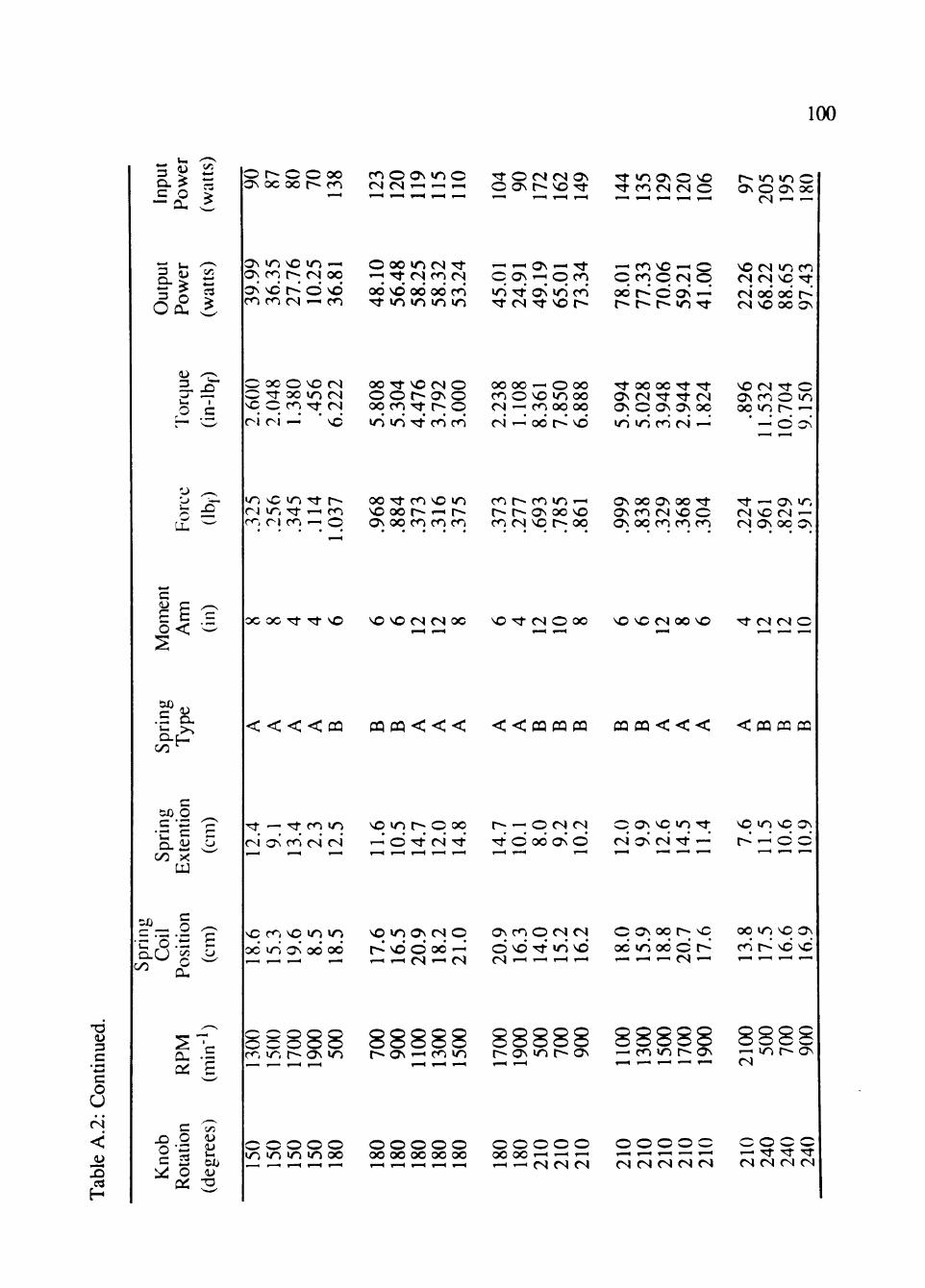
100

•a <u 3 C

•<-H *-^ c o U CN

<

ti Oi « a. t=

3 ^ «

2..0" UH I

O C

si"

o<

.5 CL

00 ^

c M) O c "z:

"C = a. H

LU

^— § •u p .t: cxU ^ ^ S.

r— r-

o

p o

X)

o C

c o

tati

o cci

c/5 ri CN Tf '-J Tf CN ro CN od vd od od ro Tf lO »0 in in

— ^ ON -^ Tf O Oj ""I p ro in rf ON in ro Tf CN Tf VO r-

'- ro VO O p ro p CN p od r- C ON *

r^ r- r^ in Tf

O oo O VO CN O Tf 00 in CN vC O CO Tf CN

00 Tf VO CN O O O t^ ON o oo ro Tf t^ O

oo oo O oo ro o VO in oo fv| -^ ro oo oo

Tf oo oo Tf Tf Ov CN Tf Tf CN ON O 0\ ON OO

Cl Cl ^ VO i n i n T f c o r o cN' -^oor-vo i n i n r o c N ^ -

in vC in Tf r^ rj in Tf T—1 CO r<, rt ro -^ O

oo Tf CO VO m VO oo r^ r^ ON oo CO CO CO

CO r^ CO in H r^ r^ Ov oo VO CO CN VO r^ oo

ON oo 0> oo Tf Ov CO CN vO C ON OO CO CO CO

r>- »n in o ON O ON oc

CN —

VO CN in CO CN CN vq Tf CN od od r^ CN VO oo ON

VO (N Tf C ON CO o in 00 in r- ^ * —"' d o

Tf ON in CN VO CN — CN Ov OO ON

O C O C T f T f v O VOVOCNCNOO V O T f C N O O O VOvOCNOOVO T f c N C N O

< < < < CQ C Q C Q < < < < < CQ CQ CQ CQ PQ < < < < PQ CQ CQ

Tf — Tf CO i n CN ON CO CN CN

VO i n r - o 00

--«* d T f CN Tf

r - — O CN CN Tf d od ON d

o o N v o i n T f voinvooN CN ON CN Tf —* r- d O

vO CO VO in »n od in ON od od

vq in ON CN p r- vd d od ^ ^ -^ CN CN

Ov CO p CN CN d vd Tf in vd CN ^ '—• '-'

r<. in r-> ON m r* ON ro m r-- ON in r^ ON

O ON oo [ vC od in od d t^

^ ro m r^ ON

oo in VO ON ro r- vd vd

^ in r^ ON CN

O O O O O i n i n i n i n oo

O O O O O oo oo oo oo 00

O O O O O oo oo 1—I ^ .—1 r-H r. CN CN CN

O O O O O CN CN CN CN CN

^ Tf ^ ^ CN CN (N CN

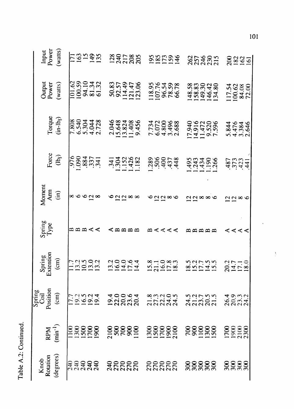
101

3 (U «2

VH I

<1^ ^ - v

O

c

o<

.5 a,

oo

c

60 O

00 X

W

—' ro in ON in r^ vo '- Tf CO

fN ON O Tf CN vO in »-i CO CO • • • • •

— O T^ .-H O O ON 00 VO

OO o r OC in CN Tf —. o o —' CN CN CN CN

CO I— ON r* vO 0C5 in Tf Tf o d CN Tf ' CO in ON CN CN

in in ro Ov VO ON oo r- in Tf

in VO Tf ON oo ON r^ in in r^ od r«.* vd od VO '—' o Ov r«- vo

CN r-* VO o in VO in Tf CO '—I CN CN cs cs CN

00 CO O CN O in 00 CO Tf oo od od ON vd Tf Tf in Tf Tf CO

O CN (N « O oo VO vO CN — — —

Tf CS OC O in VO o o r- d Tf rs — O 00 t^

00 O Tf Tf oo O Tf o Tf CN oc in CO o r-r^ vd in Tf r4

VO oo Tf oo VO Tf Tf rs o in O VO oo Tf Tf

Tf cs O VO 00 ro r- O ON oo r^ o 00 Tf VO

O VO CN O VO Tf -H r- CN Ov ON ON Tf in in

Tf VO Tf VO Tf r-- 00 Tf oo Tf CO VO ^ | f J ^ ; ^ O N r-voTfcocN r^Tfr-^ovr^ inTfcor4

vC o Tf r- -^ r-- ON oo CO Tf ON O oo CO CO

— Tf <N VO CN Tf o in CS OO CO ro -^ Tf ^

ON VO O r- oo oo O O CO Tf CN in Tf Tf Tf

in CO Tf o VO ON Tf CO ON VO Tf CN Tf CN

r CO m — oo r- cj Tf Tf ro Tf Tf

oc VO VO CN oo VO CN CN oo oc VO cs CN oo VO CS CS OO OO vO CN CN 00 VO

E

^ - o •CO.- c

CQ QQ PQ < < < CQ CQ PQ CQ pQ < < < < pQ OQ CQ CQ CQ < < < <

r cl in p CN — CO d ro ro

CN p p vq Tf CO vd Tf r^ Tf

oc H O oo CO

in ^ VO r^ oo in CN r^ in in od in r^ Tf in

CN r^ — O Tf r- oo CN — —

T3 1> 3 C -t.^

C O U C J

<

X) ,"= H

JO

o C ^

S OH oii,

c O

*-> O rf.

,—^ 1

c ^

^ ^

c/5

VH

00 (U -o ^^

r- Ol in CN Tf r-* ON vd ON ON

Tf p p vq Tf ON CN O ro d '^ CN CN CN CN

— CO in r^ ON —' in r-~ ON cs -

00 CO CN o in —<' r- CN Tf Tf <N CN CN CN CN

CO in r^ ON —I

in CN r^ in in Tf rJ CO d ^' CN CS CN CN CN

Tf ON CO (N vd d CO Tf CN CN (N CN

r^ ON ^ ro in r»- CN CO — '^ CN CN

: O O O O TT Tf Tf Tf Tf rJ (N CN CN CN

OOOOO Tf r«. r-. r^ r-CN CN CN CN CN

OOOOO r- r^ t^ r- r^ CN CN CN CN CN

8 CO CO CO ro CO CO CO CO CO

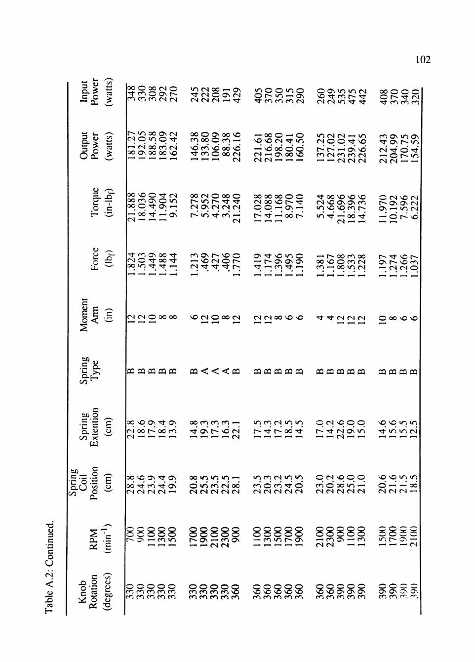
102

3 

3 43 c/5

*-• 5 TS

0(2 1

V H I

1> .—,

U H ^

c

OO O OO CN O Tf CO o Ov r -co CO CO cs CN

r-> i n oo ON CN CN p i n o Tf

^ CN od CO CN oo Ov oc oc VO

i n CN 00 — Ov Tf cs O ON CN CN CN CN T f

OO O ON OO VO ro oo O ro '— vd CO vd od VO Tf CO o oo cs

in o O in o O r^ in ON Tf CO ro ro CN

^ oo O - O vq vq cs Tf in r^ so oc G C^ CN ON 00 VO CN CN -^ r-.

O ON in in CN VO Tf CO r^ Tf CN cs in Tf Tf

in CN CN l-H in

CN o o Tf VO • • • • •

r- r o VO CO cs CO CO CN ^ ^ cs CN CN

oo O O O o r Tf r Tf CO CO CO

ro ON in ON "^ ON r- in CN Tf d Tf - o r- in CN CN -^

oc VO O Tf cs OC CO ON O in oc O Tf Ov

'- OC Tf r-H ON

oo CN O 00 O r- in r»- Tf Tf CN Ov CN CN CN t^ in Tf CO '—

cs

00 oo 00 o O CN oo VO r^ Tf O O -- ON r^ Tf oo r*»

Tf oo VO VO VO CN VO ON ON CO in VO VO CO r-in Tf oo Tf

cs -H

O CN VO CN r- Ov ON CN Ov'—1 in CN ^ o r VO

Tf r<, ON oo Tf CN O Tf OC Tf OC in Tf Tf ,—1

CO Ov r VO o ^ VO CN o r CN Tf Tf Tf r-

ON Tf VO in O •—' r^ Ov O N ON Tf ^ CO Tf l-H

^H r^ OO CO OO oo VO O CO cs CO 00 in CN

r- Tf VO r-ON r- VO CO ^ CN CN O

C N C N O O O O C V O C N O O O C N CNCNOOvOVO T f T f C N C N C N O O O V O v O

e ^ .3 O.

00 '^

3 00 O

'C = a. iii 00 X

£

60 — O C ."3 .^ c o .ti

£

T3 3 C 'S C O U (N

<

X) a H

X5

o c t^

s O-Q:

c O

O fy,

^—V

t

h

Vi

00 <u "O ^—'

CQ PQ QQ PQ PQ PQ < < < PQ PQ PQ PQ pQ PQ CQ pQ pQ CQ PQ CQ CQ CQ CQ

o c v o o v T f O N o o r o r o r O ' — '

CN oc r- 00 ro Tf Ov r^ VO CN in ro CN in in r- Tf r- od Tf

p CN vq p p r- Tf CN Ov '' ^ ^ CN ^

vq vq in in Tf in in CN

oc VO ON Tf ON

od Tf CO Tf ON CN CN CN CN -H

OO »n «n »n .-I d in CO CN od CN CN CN CN cs

in CO CN in in

CO d ro Tf d CN CN CN CN CN

p CS vq p p ro d od in CN CN CN CN CN

vq vq »ri in d * —< od CN CN CN —

O ro in r^ ON '—I ro Ov

—' -H cs CN '-' ro in r^ ON ^H ro ON '- ro

CN CN —' in r- ON —

OOOOO CO CO CO CO CO CO CO CO CO ro

OOOO ro CO CO CO ro CO CO CO CO

O O QQ VO VO 'O 'O ro CO CO CO CO

SQ O O O VO ON ON ON

CO ro CO CO CO

O O O O Ov ON ON ON CO CO r^, (T -

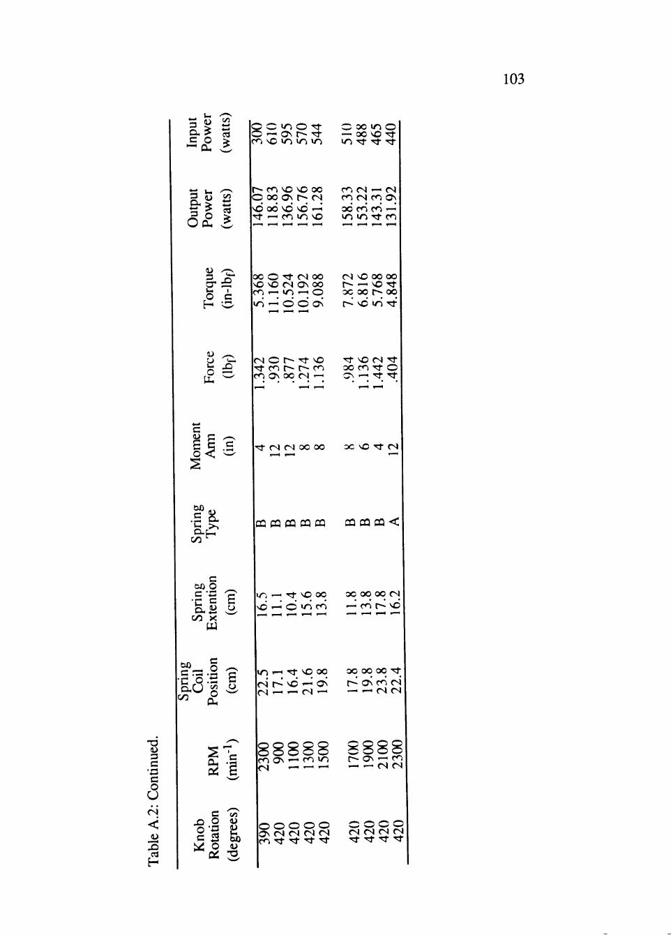
103

CX ? tS C O >

^ CU 3

c/3

VH I

o c

tu ^

Q o in o Tf O —1 ON r-« Tf CO vo in in in

r- CO VO VO oo p oo ON r- CN vd od vd vd '-3 Tf H CO in VO

oo O Tf CN oo vO vO CN ON oo CO i-< in --n Tf Tf Tf

CO CS —1 CN CO cs CO ON od CO CO ^ in in Tf CO

CN VO oo oo r- —' NO Tf oc oo r^ oo r- vd in Tf

Tf VO CN Tf oo CO Tf o ON T—1 Tf Tf

r-( 1—(

T3 <o zs a

•a c o

U • •

cs

3

c n. 00 ^

ring

nt

ion

00 X Hi

T f C S C N O C O O O C v O T f C S

QQCQCQCQPQ CQCQCQ<

£

0 0 —, o •c 'o :B £

CJ

m ' Tf VO oo sO <—1 o in CO

OC oo oc cs ^H en r^ VO

in*—iTfvooo ooooooTf csr-^vd'—'ON r~-ONrocs CN ^ ' - ' CN ' ^ — l u e s e s

C Vi

o O (O

C B bo

OS S

CO ON '—' CO i n es ^ ^ ^ r - ON ^H CO — — cs CN

O O O O O ON CN CN CN CN CO Tf Tf Tf Tf

OOOO CN CN CN CN Tf Tf Tf Tf

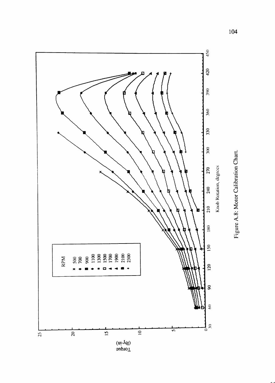
104

i /~. • ^

c CN TT

C

m

i n

o cs

o ON

03 XZ

U o r~ <N

o

o (N

O 30

•"—

•y.

' J u. SO o ^ " o

lal

OL X X

•JL

C o . H H 4 . ^

03 VH

X) _ 03

u VH

o o s

eA.8

:

V.I

3 00

(uiJqO snbjox

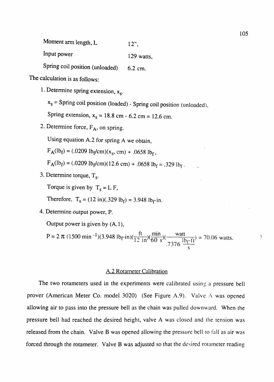
105

Moment arm length, L 12"

Input power 129 watts,

Spring coil position (unloaded) 6.2 cm.

The calculation is as follows:

1. Determine spring extension, x .

Xg - Spring coil position (loaded) - Spring coil position (unloaded),

Spring extension, Xs = 18.8 cm - 6.2 cm = 12.6 cm.

2. Determine force, F^, on spring.

Using equation A.2 for spring A we obtain,

FA(lbf) = (.0209 lbf/cm)(x3, cm) + .0658 Ibf,

FA(lbf) = (.0209 lbf/cm)(12.6 cm) + .0658 Ibf = .329 Ibf.

3. Determine torque, T .

Torque is given by Tg = L F,

Therefore, T = (12 in)(.329 Ibf) = 3.948 Ibfin.

4. Determine output power, P.

Output power is given by (A.l),

P = 2 7C (1500 min -1)(3.948 l b r i n ) ( p r [ ^ ) ( ^ ) ( ^^^^|^) = 70.06 watts. .7376 -L—

A.2 Rotameter Calibration

The two rotameters used in the experiments were calibrated using a pressure bell

prover (American Meter Co. model 3020) (See Figure A.9). Valve A was opened

allowing air to pass into the pressure bell as the chain was pulled downward. When the

pressure bell had reached the desired height, valve A was closed and the tension was

released from the chain. Valve B was opened allowing the pressure bell to fall as air was

forced through the rotameter. Valve B was adjusted so that the desired rotameter reading

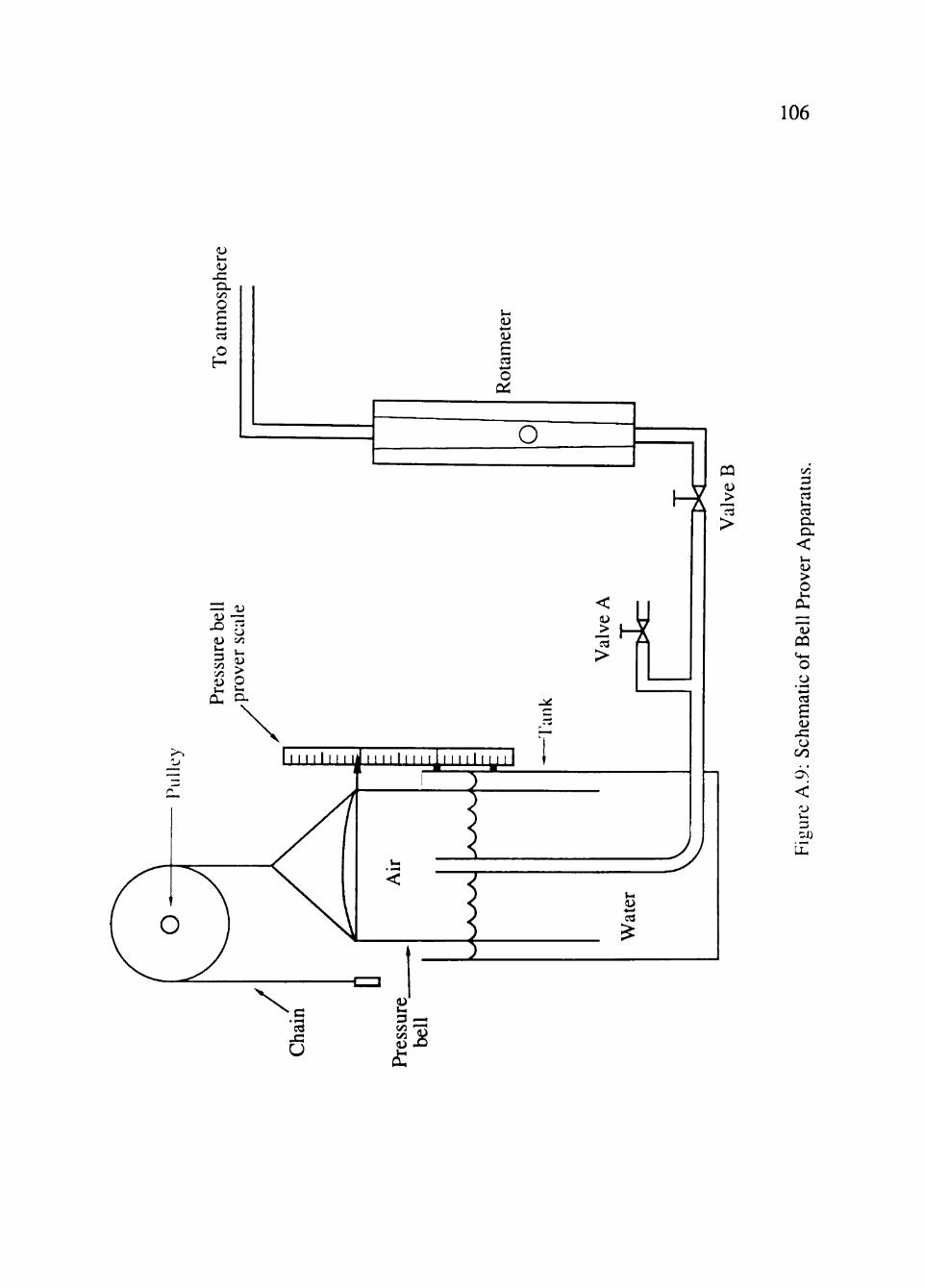
106

VH

sz a. Vi Q

a O H

VH

£ o

pti

O PQ

H ^ l >

1^ 03

>

l j ( l ' l l l M l l | l l l l l H _ l l l

t!J -<—• 03

VH

3 —. c/5 V D . O

3

VH

CX a.

< VH

> O VH

OH

CQ

o CJ

03

£ xz o 00

ON

< k.

Hi

107

was achieved. The small rotameter was read at the top of the ball. The reference gas was

air at a pressure of 100 psia and a temperature of 70T. The bell prover scale indicated the

amount of air passed which flowed through the rotameter as the elapsed time was

measured. The temperature of the air was determined by positioning a thermometer at the

outlet of the rotameter. The barometric pressure was obtained from the National Weather

Service and was 30.13" Hg during the calibration of the rotameter. Table A.3 lists the data

recorded during the nine calibration runs performed on the small rotameter.

The calculations of the air flow rate through the rotameter are as follows: Run 3 is

used as an example.

Measured quantities.

Volume of air passing through rotameter = 2.0 ft^.

Temperature = 8 r F ,

Patm = 30.13 in Hg,

Elapsed time = 7.90 min,

Rotameter indicator reading = .8 .

At this temperature from a psychromeoic chart there are 14.2 ft humid air per Ib^ dry

air and .023 Ib^ H2O per Ib^ dry air (Perry, 1984). The number of moles passing through

the rotameter is determined in the following way. Since the psychrometric chart is at

standard pressure, correct for pressure.

ft3 humid air 29.921" Hg _ ^^ ^^•^ l b n , d r y a i r ^ ^ 0 . 1 3 " H g ^ - ^ ^ - ' ^ ^

ft humid air <^^-^ Tb^" dr7air"> ("sO. T r Hg ^ = ' ^ ' " ^ lb„, dry air '

Calculate the mass of dry air passing through the rotameter,

(2.0 ft3 humid air) ( ^ \ i ' l ^ ' \ , . ) = -l^^^ ^K dry air 14.102 ft humid air

Now calculate the amount of water contained with this air,

. , ,.023 Ibm water r^r^^^^ l u U /-k

(.1418 Ibm dry air) ( ^^^ ^ "y - ) = .00326 Ib^ H2O .

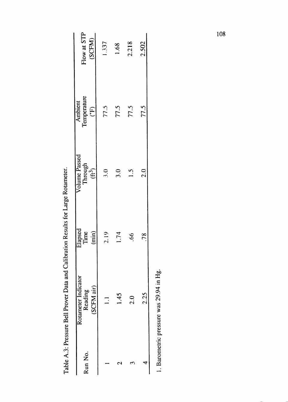
VH

£ «-> O

0^ lU OX)

53 VH

3 00 (U

a: c o 03

03

u C 03

iS 03

Q VH

> o

CQ

3 c/5 00

CO

<

03 H

OH H 0 0

03

O

u 00

c a (U 03 , ^

Xl 0) 1-^

£ & -

f2

CO 0 0 0 0

CN

CN

CN

O >o CN

T3 D Vi

-2H

CU

£

108

i~o q CO

i n q CN

^ P .£

4—>

03

c c ^

O cti

CN

^ r i

T f

r- —

so ^

•

oo r-~

•

^ Tt q — r * CN

CN

CN

O

c 3

— CN CO

c ' ^ OS OS CN Vi

3 Vi Vi lU VH

a. CJ

• ^ fa £ o J3

CQ

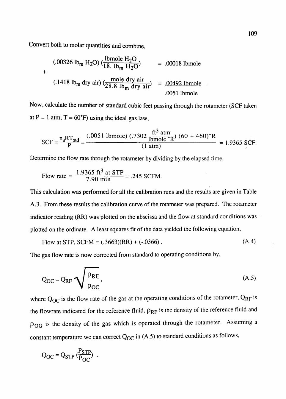
109

Conven both to molar quantities and combine,

(.00326 Ibm H2O) (igTbrnpS)^ = -^^^ ^^"^""^^ +

(a4181b,dryai r ) ( ,37;^^_;n ; ; ; ; .p = .00492 Ibmol, .

.0051 Ibmole

Now, calculate the number of standard cubic feet passing through the rotameter (SCF taken

at P = 1 atm, T = 60°F) using the ideal gas law,

„ RX (.0051 Ibmole) (.7302,/^ V"Jp) (60 + 460)'R SCF = ^ ^ & = , /*^,"^f ^ ^ =1.9365 SCF.

r (1 atm) Determine the flow rate through the rotameter by dividing by the elapsed time,

iri . 1.9365 ft at STP . . . „_„^^ Flow rate = 7 QQ ^^^ = .245 SCFM.

This calculation was performed for all the calibration runs and the results are given in Table

A.3. From these results the calibration curve of the rotameter was prepared. The rotameter

indicator reading (RR) was plotted on the abscissa and the flow at standard conditions was

plotted on the ordinate. A least squares fit of the data yielded the following equation.

Flow at STP, SCFM = (.3663)(RR) + (-.0366). (A.4)

The gas flow rate is now corrected from standard to operating conditions by,

QOC = Q R F A / ^ ^ ' ( -5) \ Poc

where QQC is the flow rate of the gas at the operating conditions of the rotameter, QRF is

the flowrate indicated for the reference fluid, pRp is the density of the reference fluid and

pOG is the density of the gas which is operated through the rotameter. Assuming a

constant temperature we can correct QQC i" (^.5) to standard conditions as follows,

Qoc = QsTP ("p^) •

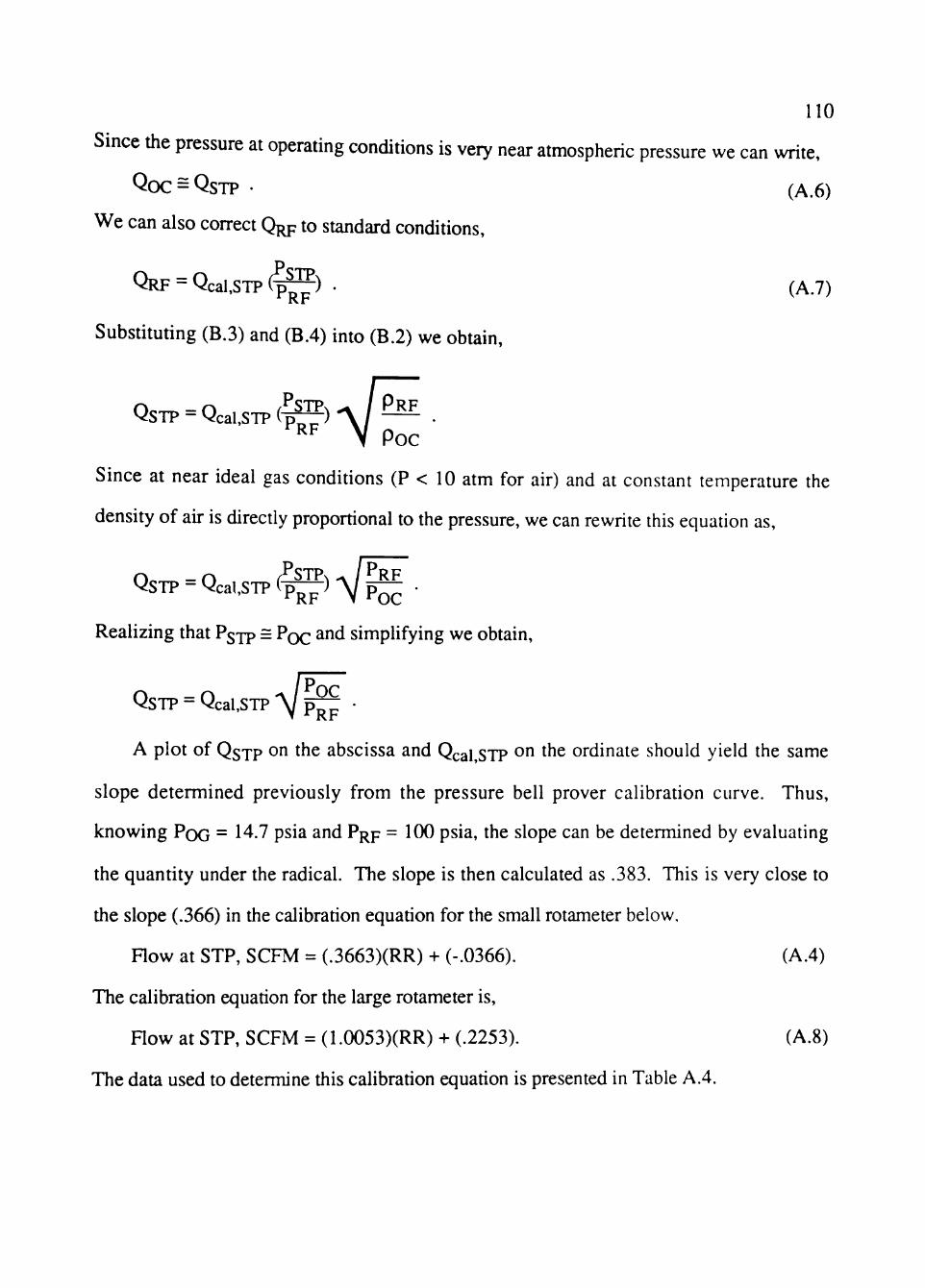
no Since the pressure at operating conditions is very near atmospheric pressure we can write,

Qoc = QsTP • (A.6)

We can also correct Q^p to standard conditions,

QRF = Qcal,STP ( ^ ) . (A.7)

Substituting (B.3) and (B.4) into (B.2) we obtain,

QsTP = Q c a l . S T p t e A / 2 ^ . ^^ \ Poc

Since at near ideal gas conditions (P < 10 atm for air) and at constant temperature the

density of air is directly proportional to the pressure, we can rewrite this equation as,

QsTP = Qca,,STT(^)Vli'-Realizing that Pgip = PQQ and simplifying we obtain.

QsTP = Qcal,STP ^ P ^

A plot of QsTP on the abscissa and Qcal,STP on the ordinate should yield the same

slope determined previously from the pressure bell prover calibration curve. Thus,

knowing PQG = 14.7 psia and PRP = 100 psia, the slope can be determined by evaluating

the quantity under the radical. The slope is then calculated as .383. This is very close to

the slope (.366) in the calibration equation for the small rotameter below.

How at STP, SCFM = (.3663)(RR) + (-.0366). (A.4)

The calibration equation for the large rotameter is.

Row at STP, SCFM = (1.0053)(RR) + (.2253). (A.8)

The data used to determine this calibration equation is presented in Table A.4.

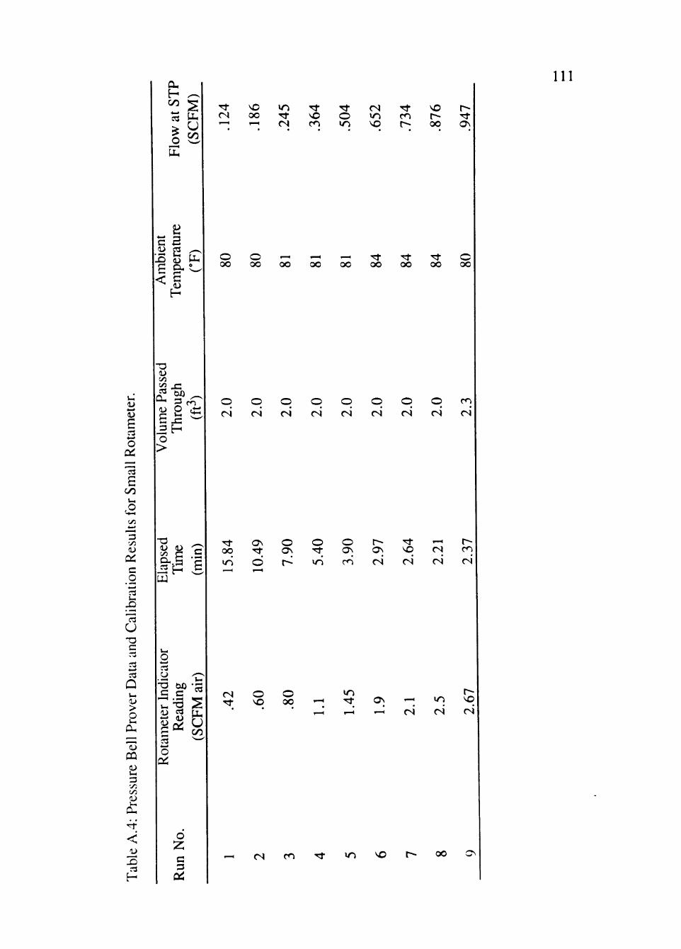
V H

 2

O H

PQ

VH

3

<

X i 03

H

111

o u 00

c (U Xi F <

a e a OH

£ H

tu

'^ CN '"'

VO OO ""l

>n -^ CN

-^ VO CO

-^ o yn

CN lO VO

'^ CO r

VO t^ OO

t^ -^ ON

O OO

O OO

.—1

oo ,-H

oo ^^ oo

rt oo

rt OO

Tt oo

o oo

oo Vi

O H

«o - xz an o

>

xz

p <£

-a ^ <U D O

til

q CN

q CN

q CN

q CN

q CN

q cs q

CN q CN

CO

CN

03

^ P 2 ^ £ " oo 3 ^^ o

o Z c 3

0C3 ON o

ON

O O ON

CO

O N

CN

VO CN

CN CN

CO

CN

CN rt •

o VO

o 00 1-H

1-H

U-) rt ,-H

ON 1-H

'~; CN

»n CN

r-VO (N

CN CO >o VO 0 0

APPENDIX B

EQUATION DERIVATIONS AND CALCULATIONAL

PROCEDURES

B.l Rate of Snlfitp, DepleHnn

The rate of sulfite ion disappearance is used to determine the rate of oxygen

consumption within the dispersion. Oxygen, which is present in the gas phase, is

absorbed into the liquid phase and reacts with the sulfite ions according to the following

half reaction,

2 SO3-2 + O2 ^ ^ • 2 SO4-2.

The rate of change of sulfite ion concentration is determined by a titration procedure using

iodine. Iodine is a moderately strong oxidizing agent and is used to titrate reducing agents

such as sulfite. These titrations are performed in solutions with pH's ranging from neutral

or weakly alkaline to weakly acidic solutions. If the titration is performed in a solution

which is too alkaline, I2 will disproportionate according to the following half reaction,

I2 + 2 OH- V ^ 10- + I + H2O .

If the titration is carried out in a solution which is too acidic, the starch which is used as an

end-point indicator tends to hydrolyze or decompose so that the end-point may be affected.

Also, in strongly acidic solutions the T produced by the reaction tends to be oxidized by

dissolved oxygen according to,

4 r -h O2 + 4 H+ 2 I2 + 2 H2O .

The titration is carried out in a mild solution of acetic acid to control the pH of the solution.

The titration procedure, shown graphically in Figure B.l, involves four solutions; (i) a

starch, acid, and water solution, (ii) the iodine solution, (in) the sulfite solution within the

112

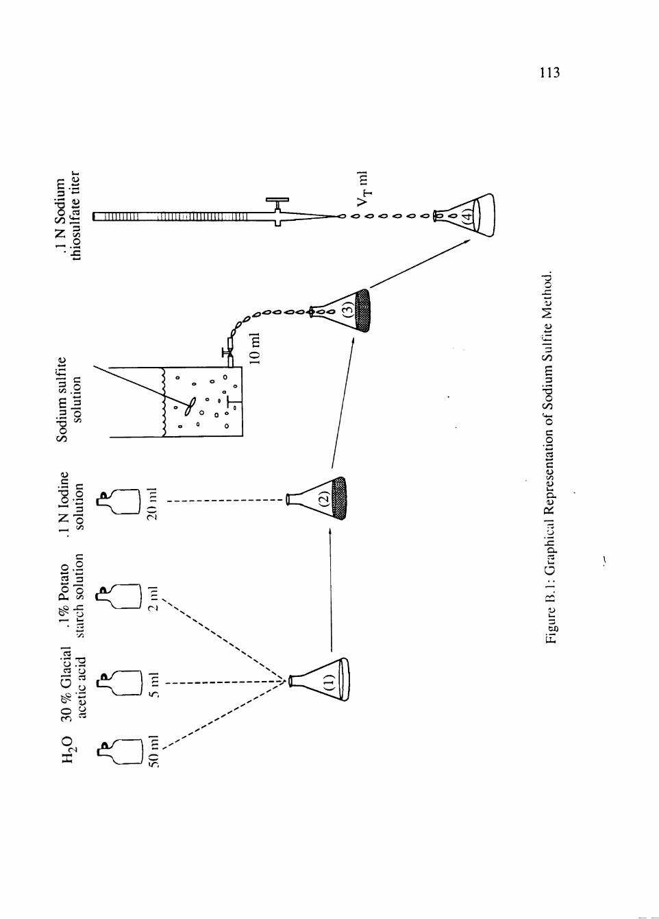
113

r* c 3

-a o 00

Z ^ • ^

'

U-i

a> 4 - ^

• • — '

.^ < * H

3

O XZ

i i i i i i i i i i i i i i i i i i ' H D <D ^ <D <D <D ^

-

. <Z)1 o

CN

X

00

£ 3

•-5 o 00

c .2 B c c/5

VH

a.

a a.

O

3 CX)

IJU

l O

114

dispersion, and (iv) the sodium thiosulfate solution. The iodine solution is prepared by

taking 50 ml of distilled water and placing it in a 250 ml Erienmeyer flask. Then 5 ml of

30% (by volume) glacial acetic acid and 2 ml of . 1 % (by weight) potato starch solution

were added to the flask. Just before a sample was taken from the dispersion, 20 ml of .1 N

iodine solution was added to the flask. A 10 ml sample of sodium sulfite solution was

withdrawn from the dispersion and added to the flask. This solution in the flask was then

titrated with the.l N sodium thiosulfate titer solution.

The rate of change of sulfite ion concentration is determined by following the sulfite

ion concentration throughout the duration of the experiment. The sulfite ion concentration

is determined by adding the sulfite solution to the iodine solution and then back-titrating the

excess iodine with the sodium thiosulfate solution.

The sulfite ion concentration is determined in the following way. A 10 ml sample is

withdrawn from the dispersion at time tj and added to the iodine solution in the 250 ml

flask. The iodine reacts with the sulfite ion according to the following half reaction,

I2 + SO3-2 + H2O • SO4-2 + 21- + 2H+.

Since the concentration of the sulfite solution is not known, let us denote the sodium sulfite

concentration as C moles/1. The number of moles of sulfite ions in the 10 ml sample is

thus,

C moles Na2S07, , _ , , _ 11 _ mole S03-^ ^ ( U^. ^ (10 " 1 ^ "- ^TOOO^^ (mole Na2S03^ =

(.01 C) moles SO3"- in sample.

The number of moles of iodine in 20 ml of the . 1 N (.05 mole I2/I) I2 solution,

/-.i , T , ^/•05 mole I2, , 1 , .001 moles IT (20 ml I2 soln.)( j ) {JQQQ^) = ^ ,^^ .^i.^i^- -

Using the fact that iodine reacts with sulfite ion in an equimolar ratio, the number of moles

of unreacted iodine is given by.

.001 moles I2 01 C moles SO3-2 1 mole I2 Hn the I2 solution^ ' ^ in the sample ^ S mole SO3--

115

)

= (.001 - .OIC) moles I2 unreacted.

Notice that if the concentration of the sodium sulfite solution in the dispersion is greater

than .1 moleA, the equation yields a negative number which means that there is no excess

iodine present in the flask. So, let us suppose the sample withdrawn from the tank had a

sulfite ion concentration such that [Na2S03] < .20 M. The solution of excess iodine is

now titrated with the solution of .1 N sodium thiosulfate. The iodine reacts with the

thiosulfate ion according to the reaction,

.5 I2 + S203-2 • r + .5 S406"^.

The amount of . 1 N (.05 mole Na2S203/l) sodium thiosulfate titer used (Vy ml) to titrate

the excess iodine is given by,

./^/^, /^,^ , x x.moic S2O3-2, mok Na2S203,, 1 ,,1000 ml, (.OOl-.OlC moles l2)( .5 mofe I2 ^ mole S203-^^^-Q^ "^^le Na2S203^(Tl^hr)-

This is reduced to,

Vx = (40-400C). (B.l)

Now another sample from the tank is taken at time t2 and let us assume the

concentration within the tank is now C+AC, where AC is the change in sulfite concentration

between samplings. The amount of sodium thiosulfate solution used to titrate the sample

taken at t2 is therefore,

VT 2 = (40 - 400(C+AC)). (B-2)

Rearranging, (B.l) and (B.2) we obtain,

40 - 400C - VT,I = 40 - 400(C + AC) - VT,2 = 0 ,

Solving for AC we obtain.

116

Substituting AVT = iVj2" "^T,]) and At = t2 - tj and dividing botii sides by At we obtain,

AC^ 1 AVj At ~ • 400 At '

and at the limit as At —> Q,

d C _ 1 dVj dt "400 dt •

Since C represents the concentration of sodium sulfite in the sample and 1 mole of Na2S03'

^ contains 1 mole of 803'^, we can write,

d[S03-^] 1 dVy dt " ' 4 0 0 dt • (^•' )

Thus, the equation above represents the rate of change of sulfite ion concentration

expressed in terms of the rate of change in the sodium thiosulfate titer used. The term

dVj/dt is determined by plotting the volume of sodium thiosulfate titer used (ml) versus the

sampling time (min) and determining the slope (ml/min).

B.2 Determination of Henrv's Law Constant

The Henry's law constant is needed in the calculations for the mass transfer coefficient

(See equation (2.33)). It relates the partial pressure and the concentration at equilibrium

by,

P02 = H C02.

Since the solubility of oxygen in water varies with temperature, the constant is a

function of temperature. For a given partial pressure of oxygen the concentration of

oxygen in water is obtained from oxygen solubility data. Table B.l lists the solubility of

oxygen at various temperatures at an oxygen partial pressure in air of .209 atm.

The Henry's law constants were calculated for the temperature range at which the

experiments were conducted. They were then fitted according to an Ahhrenius expression,

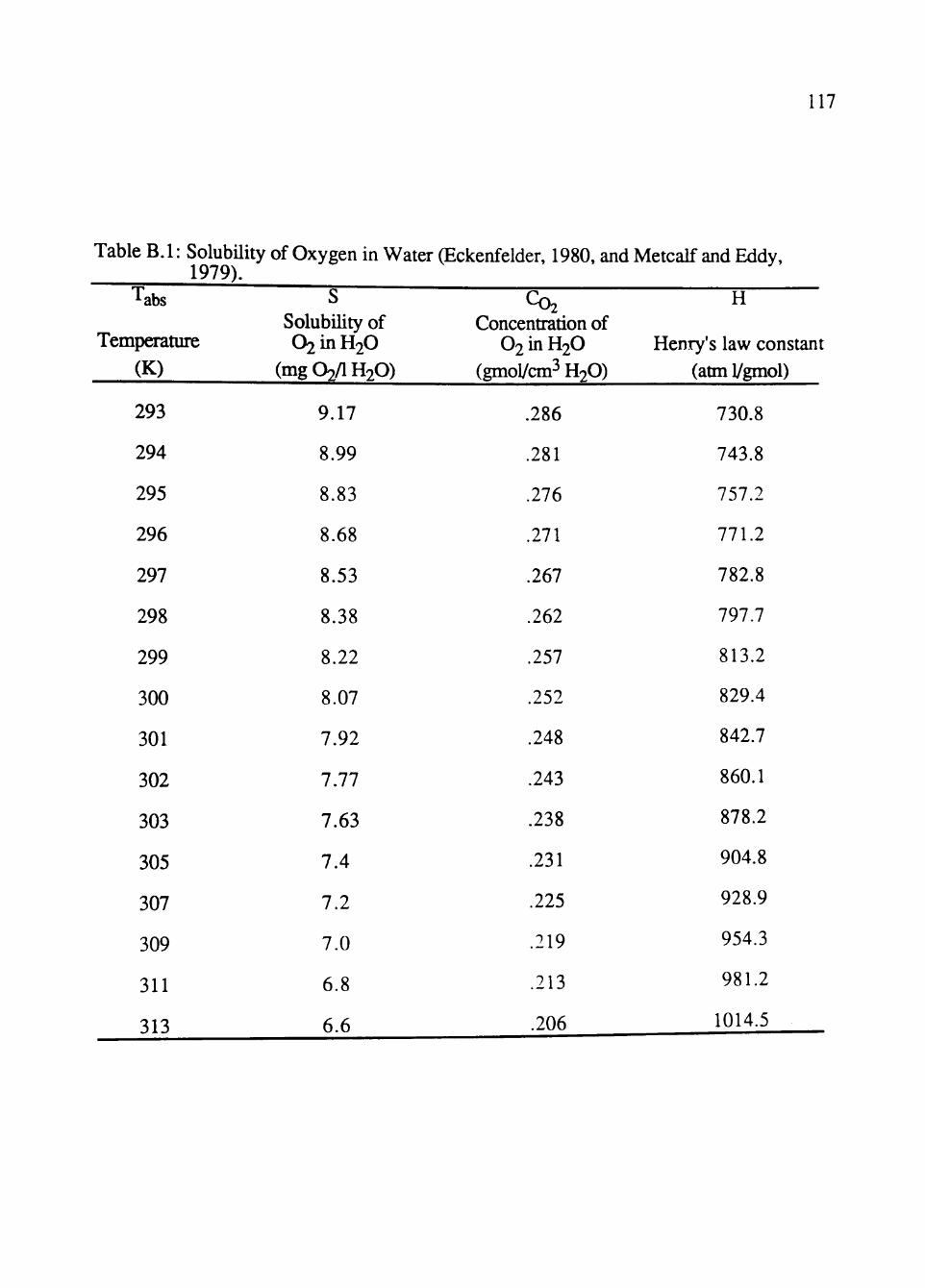
117

Table B. 1: Solubility of Oxygen in Water (Eckenfelder, 1980, and Metcalf and Eddy, 1979).

Tabs S C02 H Solubility of Concentration of

Temperature O2 in H2O O2 in H2O Henry's law constant (K) (mg O2/IH2O) (gmol/cm^ H2O) (atm 1/gmol)

293 9.17 .286 730.8

294 8.99 .281 743.8

295 8.83 .276 757.2

296

297

298

299

300

301

302

303

305

307

309

311

313

8.68

8.53

8.38

8.22

8.07

7.92

7.77

7.63

7.4

7.2

7.0

6.8

6.6

.271

.267

.262

.257

.252

.248

.243

.238

.231

.225

.219

.213

.206

771.2

782.8

797.7

813.2

829.4

842.7

860.1

878.2

904.8

928.9

954.3

981.2

1014.5

118 H = A H e -(En/RTabs)

" ' (B.5)

where A H is a pre-exponential factor (atm 1 / mole) and EH is the apparent activation energy

O cal / mole) of solution. By rearranging,

and plotting In H versus lA^^bs the parameters EA and AH can be determined. A least-

squares fit yield the following equation.

In H = (-1508.807 K) i ^ ) + (11.7469).

or.

^abs

,1508.807, H = 126,361 e - ( " ^ ; ) T ' ' (B.6)

abs

and,

EA = 2.998 kcal / mole ,

which indicates that H is a weak function of temperature.

B.3 Determination of the Average Partial Pressure of Oxygen

This section lists the assumptions and summarizes the procedure for calculating the

average partial pressure of oxygen in the dispersion. The following quantities are known

(See Figure B.2): inlet gas flow rate (Qg,in), inlet gas pressure (Piniet), atmospheric

pressure (Patm)' average dispersion temperature (T^vg), ambient temperature (Tamb), inlet

partial pressure of oxygen (po2,in)' oxygen consumption rate ((- ro2 ) D ) ' ^"^ the

dispersion volume (V^). The average dispersion temperature is determined by taking a

numerical average of the dispersion temperatures during the experiment.

Taking the control volume to be the liquid in the tank, a molar balance over oxygen

gives,

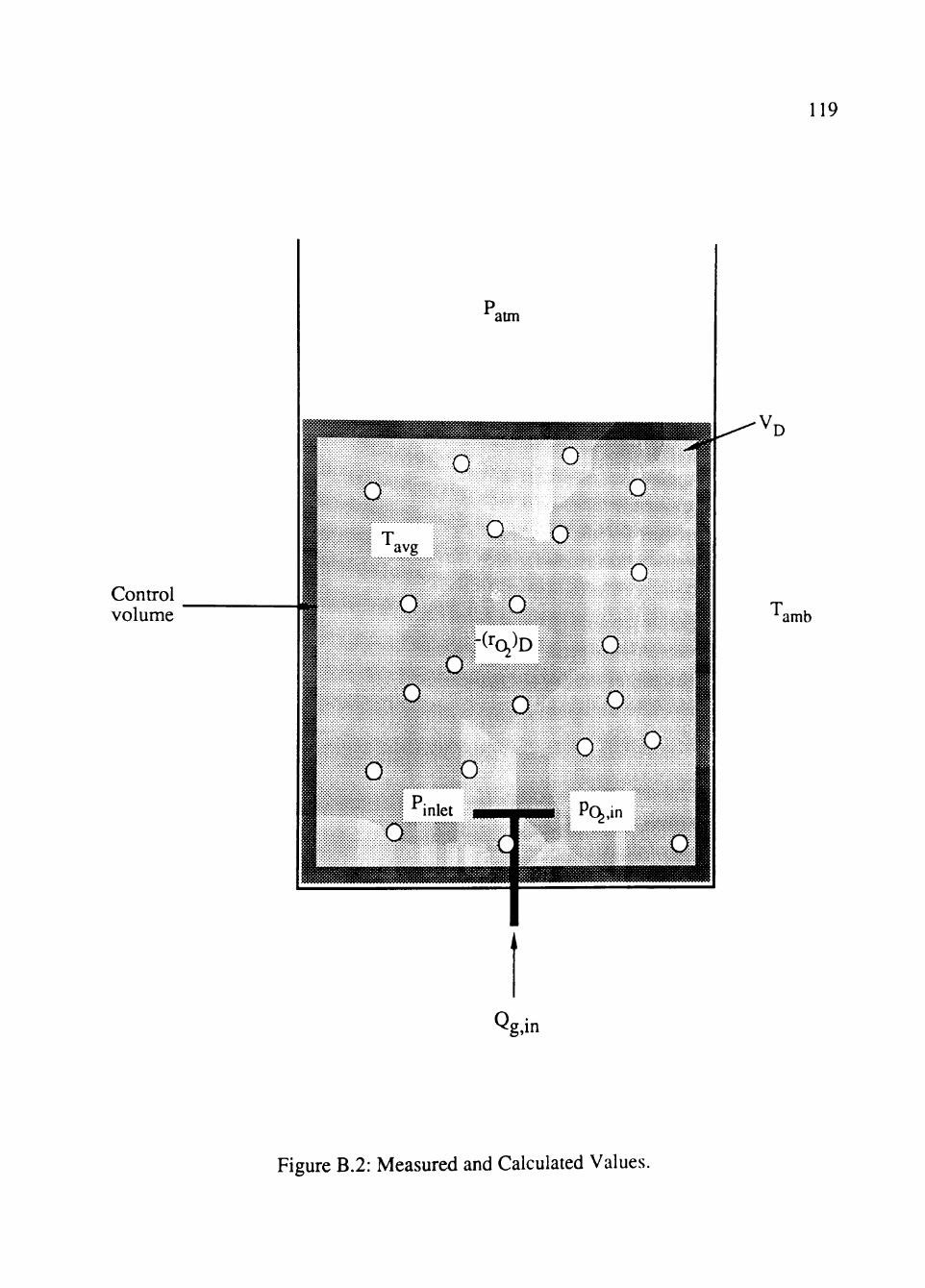
119

Control volume

1 1 T

1 ^ 1 ^ 1 1 ' P" 1 *-'

P

0

o

o -(ro,)D

0

o

o ilet mmmmt

^ 1 0 1 o

0 1 0 0 1

• Pq.in 1

o |

T amb

'g,in

Figure B.2: Measured and Calculated Values.

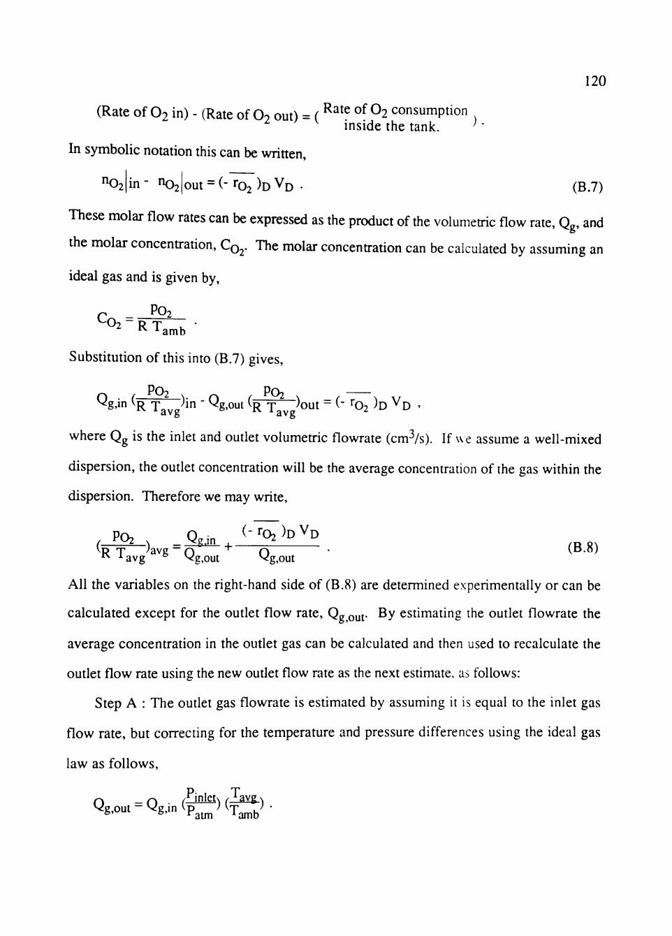
120

(Rate of O2 in) - (Rate of Oo out) = ( ^^^^ °^ ^2 consumption inside the tank. ^ •

In symbolic notation this can be written,

t 02 in - "02 out = (- ro2 )D VD • (B.7)

These molar flow rates can be expressed as the product of the volumeuic flow rate, Qg, and

the molar concentration, C02. The molar concentration can be calculated by assuming an

ideal gas and is given by,

PO2

Substitution of this into (B.7) gives,

^g,in VR Tgvg in • g.out R TavgÔ"t - (" Oz )D v D ,

where Qg is the inlet and outlet volumetric flowrate (cm^/s). If we assume a well-mixed

dispersion, the outiet concentration will be the average concentration of the gas within the

dispersion. Therefore we may write.

Pru O " ^07 )D VD VD T avg ~ o O vt>.o; ^ âvg ° ^g,out ^g,out

All the variables on the right-hand side of (B.8) are determined experimentally or can be

calculated except for the outlet flow rate, Qg out- ^X estimating the outlet flowrate the

average concentration in the outiet gas can be calculated and then used to recalculate the

outlet flow rate using the new outiet flow rate as the next estimate, as follows:

Step A : The outiet gas flowrate is estimated by assuming it is equal to the inlet gas

flow rate, but correcting for the temperature and pressure differences using the ideal gas

law as follows,

Q - o • f inletA / J W \ Vg.out ~ Vg,in Vp M y J •

*' * âim âmb

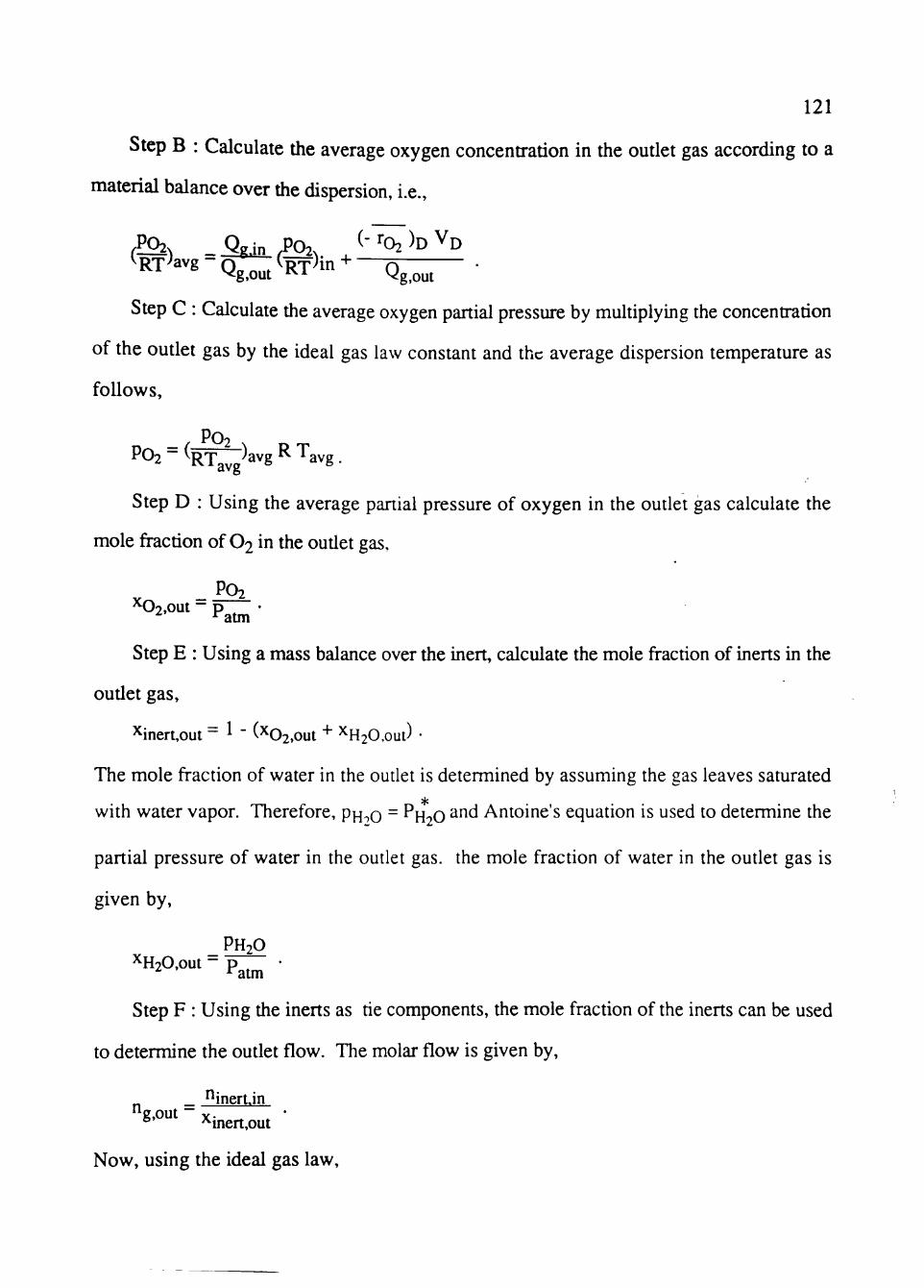
121

Step B : Calculate the average oxygen concentration in the outiet gas according to a

material balance over the dispersion, i.e..

^ R T W Qg,out^RT>in+ Qg^^^ •

Step C : Calculate the average oxygen partial pressure by multiplying the concentration

of the outlet gas by the ideal gas law constant and the average dispersion temperature as

follows.

Step D : Using the average panial pressure of oxygen in the outlet gas calculate the

mole firaction of O2 in the outiet gas,

PO2 ^02,0Ut ~ p •

âtm

Step E : Using a mass balance over the inert, calculate the mole fraction of inerts in the

outiet gas,

'înert,out ~ ^ " v^02,out " H20,out) •

The mole fraction of water in the outlet is determined by assuming the gas leaves saturated

with water vapor. Therefore, PHOO ~ PH2O ' "^ Antoine's equation is used to determine the

partial pressure of water in the outlet gas. the mole fraction of water in the outlet gas is

given by,

PH2O ^H20,out - p ^ âtm

Step F : Using the inerts as tie components, the mole fraction of the inerts can be used

to determine the outiet flow. The molar flow is given by,

_ "inertin "g.out ~ Y-® 'înert,out

Now, using the ideal gas law.

122

Q _ "g.out R l^avg g.out-— p - ^ .

^atm

Step G : Now, check to see if the outiet gas flow rate calculated in step F is within

.005% of the outlet flow assumed in step A. If it is, use the average partial pressure of

oxygen calculated in step C. If it is not within .005%, use the outlet flow calculated in step

F as the new value for the flow and repeat with step B.

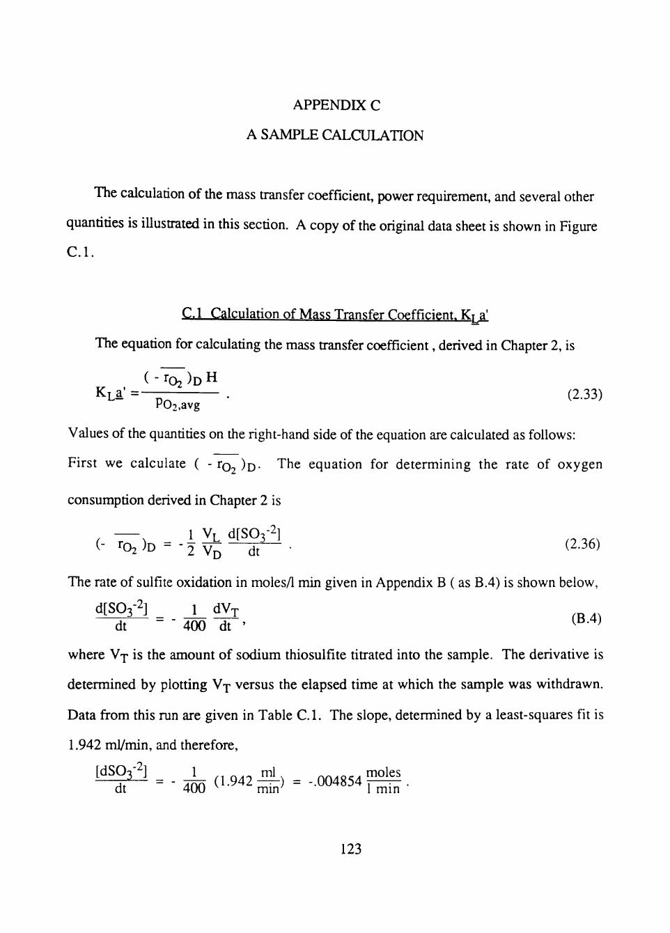
APPENDDC C

A SAMPLE CALCULATION

The calculation of the mass transfer coefficient, power requirement, and several other

quantities is illustrated in this section. A copy of the original data sheet is shown in Figure

C.l .

C. 1 Calculation of Mass Transfer Coefficient. K^a'

The equation for calculating the mass transfer coefficient, derived in Chapter 2, is

( - ro2 )D H K L I ' = - r - . (2.33)

F02,avg

Values of the quantities on the right-hand side of the equation are calculated as follows:

First we calculate ( - ro2 )D- The equation for determining the rate of oxygen

consumption derived in Chapter 2 is

'- ^ '-^^^ . (2.36) (- ro2 )D - - 2 VD dt

The rate of sulfite oxidation in molesA min given in Appendix B ( as B.4) is shown below,

d[S03-'] ^ d V r dt " • 400 dt ' ^^-^^

where Vj is the amount of sodium thiosulfite titrated into the sample. The derivative is

determined by plotting V-j- versus the elapsed time at which the sample was withdrawn.

Data from this run are given in Table C.l. The slope, determined by a least-squares fit is

1.942 ml/min, and therefore,

i ^ ^ = - j i x ( 1 . 9 4 2 ^ ) = - . 0 0 4 8 5 4 = ^ . dt 400 ^ min^ 1 min

123

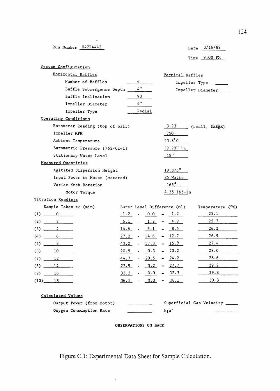
124

Run Number H42R44^2

System Configuration

Horizontal Baffles

Number of Baffles _

Baffle Submergence Depth _

Baffle Inclination _

Impeller Diameter _

Impeller Type _

Operatine Conditions

Rotameter Reading (top of ball)

Impeller RPM

Ambient Temperature

Barometric Pressure (762-0141)

Stationary Water Level

Measured Quantities

Agitated Dispersion Height

Input Power to Motor (metered)

Variac Knob Rotation

Motor Torque

Titration Readings

Date 3/16/89

Time 9:00 PM

Vertical Baffles

Impeller T>'pe

4" Inpeller Diameter

90

Radial

3.23 (small, XSJLP)

750

23.8 C

29.90' r.2

18"

19.875"

85 Watts

165'

4.55 Ibf-in

CD (2)

(3)

(A)

(5)

(6)

(7)

(8)

(9)

(10)

Cs

Jample Taken a t

0

2

4

6

8

10

12

14

16

18

i lcu la ted Values

Buret Level Difference (ml)

1.2

6.1

14.6

27.3

43.2

20.5

44.7

27.9

32.3

36.1

0.0 1.2

1.2

6.1

14.6

4.9

8.5

- 12.7

Temperature (°C)

25.1

25.7

26.2

26.9

27.3 - 15.9 27.4

0.3 - 20.2 28.0

20.5 - 24.2 28.6

0.2 - 27.7 29.2

0.0

0.0

32.3

36.1

29.8

30.3

Output Power (from motor)

Oxygen Consumption Rate

Superficial Gas Velocity

k^a'

OBSERVATIONS ON BACK

Figure C.l: Experimental Data Sheet for Sample Calculation.

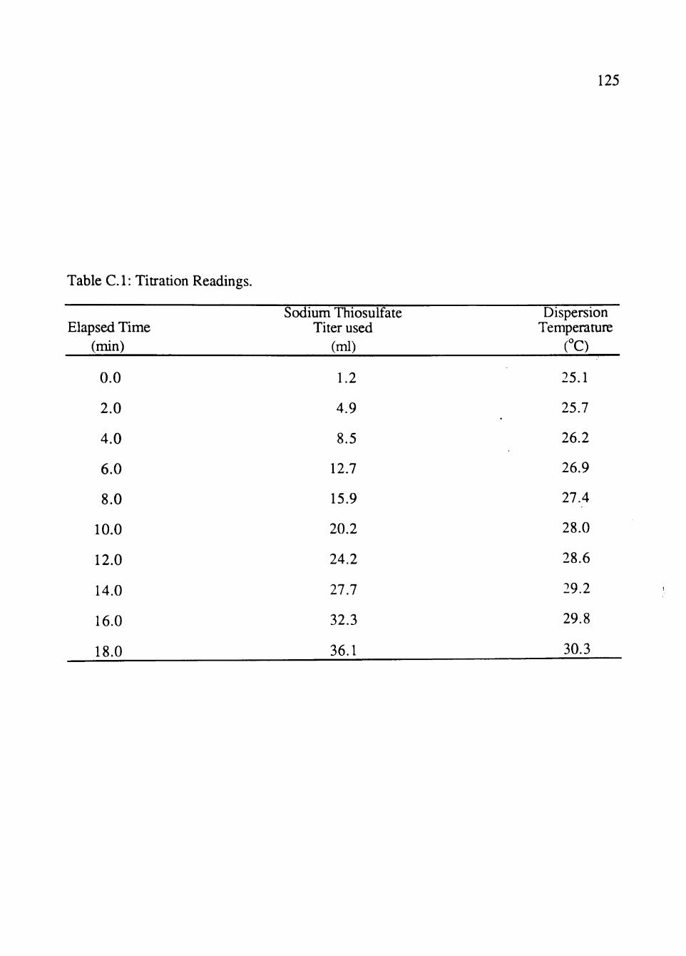
125

Table C.l: Titration Readings.

Elapsed Time (min)

0.0

2.0

4.0

6.0

8.0

10.0

12.0

14.0

16.0

18.0

Sodium Thiosulfate Titer used

(ml)

1.2

4.9

8.5

12.7

15.9

20.2

24.2

27.7

32.3

36.1

Dispersion Tempera tuns

CO

25.1

25.7

26.2

26.9

27.4

28.0

28.6

29.2

29.8

30.3

126

The liquid volume is given by,

VL = 7 r ( | ) 2H = ; t ( l M 5 u i ) 2 ( j g o i „ ) m3 ^ ^ ^ ^ ^ ^ 3 ^ 61,023.5 in-

and die dispersion volume is given by,

VD = 71 (^)2 HA = 7C ( i ^ ^ ) 2 (19.875 in) ( T T T I ? ^ ) = -0353 m3 . ^ ^ 61,023.5 in^

By substituting all these quantities into (2.36) gives,

(- " ^ > D = - \ -^^—l (-.004854 3 ^ ) = .002198 2^?l£i02 ^ 2 0353 m- 1 min^ 1 mm

Next we calculate the value of Po2,avg- Assuming that the gas in the tank is well-

mixed, Po2,avg is taken as Po2,out- '^^is quantity is obtained by iteration as described in

Appendix B. The relevant quantities are as follows:

Inlet pressure is determined by taking into account the barometric pressure and the

hydrostatic head above the sparger ring. Since the sparger ring is 2" (.167 ft) above the

tank base the inlet pressure is,

( H s - . 1 6 7 ) P H 2 0 g ^inlet ~ ' atm ••" a '

(1 .5- .167)f t (62.2yf) (32 .174^)

Pinlet = 101.254 kPa . , ^ ^ . . i b l - f t ^ 7 7 ^ ' 3 2 . 1 7 4 ' - ^ 20.885*-^

Ibf s2 ft2

Pinlet = 105.225 kPa .

The inlet air flow rate (at STP) was determined from the rotameter reading. For the

rotameter reading RR = 3.23,

Qg,in = (RR)(.3663) - (.0366) = (3.23)(.3663) - .0366 = 1 - 1 4 7 ^ . (A.4)

Now, to correct the pressure and temperature to the experimental conditions, it was

assumed that the inlet air enters the sparger ring at ambient temperature.

127

O - o ^amb Pstd , .y. ft . 296.95 K, , 101.325 kPa. . . . . ft Vg,in-^g4n 7^^ Piniet" min ' 288.7 K ^ M05.225 kPa ^ " ^-^-^^min '

The molar flow through the rotameter is given by,

p,„,^,Q^,„ (105.225 Pa) (.000536 g^) ^^.es a.r

(8.314 ^ 3 f | ) (296.95 K)

Now, taking the inlet air composition as 20.946% oxygen and the balance inerts, the

component molar flow rates are,

"02,in = (.20946) (.0228 moles air/s) = .0478 moles O2/S,

"inert,in = (.79054) (.0228 moles air/s) = .0181 moles inen/s,

and the partial pressiu^es are,

P02,in = X02 Pinlet = (-20946) (105.225 kPa) = 22.040 kPa,

Pinert = inert Pinlet = (.79054) (105.225 kPa) = 83.184 kPa.

The time-average dispersion temperature was calculated by,

^ Zi=l ^ i where tj is the elapsed time between sample i and sample i-1, tf is the total elapsed time of

the run, and Tj is the temperature of the dispersion when sample i was withdrawn. For this

run, N = 10, tf = 20 min.

^ N Ii=l ^-^ Atj = 554.4 °C min.

and,

Tavg = ^^zOm^n""'" = 27-72 'C = 300.87 K.

The average outiet partial pressure of oxygen is now calculated by using the iterative

procedure described in Appendix B:

128

Step 1. Taking the outiet volumetric gas flow as equal to the inlet gas but corrected for

temperature and pressure differences,

O - o r inlet fj^s .n^^f.^^\ . 105.23 kPa 300.87 K _ . . 0 0 ^ Qg.out - Qg,in ip^) ij^) - (1.136 ^ ( jQ^ 25 kPa^(296.95 K " ^'^"^ min '

Step 2. Using the rate of oxygen consumption and solving for (P02/^Tavg)avg we

obtain,

( ^^2 s _ vg,in / ^<J2 V t (B 8) ^RT,,gâvg - Qg ^ ^ ^RT^bîn + Q^^^^^ • ^ • >

The calculation of tiie inlet concenttation , (p02/RT)in, is calculated under tiie assumption of

thermal equilibrium with the surroundings,

( PO^).^ = 22,040 Pa ^ ^^^1 mole/m3. ^RTamb in (8314 m^Pa/mole K)(296.95 K)

Substituting into (B.8),

1 1 3 6 i t l , (2.198 5 ^ ) ( . 0 3 5 3 m 3 )

( ^ ) a v g = - ^ (8-927 3 ^ ) '^^^^^ = 6.164 " ^ . ^ " 1 . 2 0 0 ^ -' . 0 3 4 0 ^

Step 3. Calculate the average partial pressure given by,

PO2 POzavg = ^RTavg ^ S âvg'

taking the temperature to be the average dispersion temperature, T^vg. So, using,

P02.avg = (6.164 ^ ) (.008314 m^ ^ ^ ^ )(300.87 K = 15.474 kPa.

Step 4. Calculate the mole fraction of oxygen in tiie outlet gas. This is calculated by,

_ P02,avg _ 15.474 kPa _ .^^^ xo2,out - p^^^ - 101.254 kPa ~ •^^^*-

Step 5. Using an inert balance, determine the mole fraction of inerts in the outlet gas.

An inert balance gives,

Xinert,out ~ 1 " (^02,oul •*" ^H20,out)-

129

The mole fraction of water in the outiet is determined by assuming the outlet gas is

saturated with water vapor. Therefore, PH2O = P*H20' ^^^ Antoine's equation can be used

to determine the partial pressure of the water vapor in the outiet gas,

LogioP*H20 = 8.10765 - ( j + 235.0) '

where tiie temperature, T, is in °C, P*H20 is in mm Hg. For T = 300.87 K,

LoglOP*H20 = 8.10765 - (27.72 °C +235.0) " ^^^'^^^

So,

P*H20 = PH2O = 29.680 mm Hg = 3.957 kPa.

The mole fraction of the water in the outlet gas is given by,

PH2O 3.957 kPa _ XHzCoui - p^j^ - 101.254 kPa " •^^^^•

Now, using the inert balance,

Xinert,out = 1 - (-1528 -H .0391) = .8081.

Step 6. Use the inerts as a tie component to determine the molar outlet flow,

^inertin "g.out - X- * . • ** ^inert,out

And using njngrt,in = -0181 moles/s and Xing out = -8081,

. 0 1 8 0 ^ ^ ^ s_ _ mole

ng,out- 8081 -'^^^^ s •

The outiet flow rate is

D T (1.341 ^ ^ ) ( . 2 9 3 6 ^ V ^ ^ ) ( 3 0 0 . 8 7 K) .3 r» n^.outRTavg ^ "^ mm-'^ mole min^^ 1 ^ 1 1 7 4 ^ ^ ^g.out- p^^^ - 101.25 kPa ' ' ' ^ m i n '

Step 7. Check to see if the calculated outlet flow is within tolerance to the outlet flow

guessed in Step 1. If it is not within tolerance, repeat these calculations using the outiet

130

flow calculated in Step 6 for the guess in Step 1. The tolerance chosen is .005% the value

of the calculated flow:

Tolerance = .00005 (1.174 ^ )= .0000587 4 - . mm' mm

Check the tolerance:

I I f t3

I Qg,out (calculated)-Qg,out(guessed)| < .0000587 ^ - j ^ ?

Substituting, we obtain,

ft ft ft 1 . 1 7 4 - ^ - 1 . 2 0 0 - ^ = - . 0 2 6 - ^ . inin min min

ft ft Is -.026 —^ < .0000587 —^ ? No, so go through second iteration. For subsequent min mm ' & & ^

iterations the guessed volumetric flows, and outiet oxygen partial pressure are shown

below.

ition

1

2

3

4

5

Guessed Volumetric flow

(ft^/min)

1.200

1.174

1.179

1.178

1.178

P02,0Ut

(kPa)

15.47

15.82

15.75

15.76

15.76

The average outlet partial pressure P02,avg' is thus equal to 15.762 kPa.

The Henry's law constant is calculated using,

TT 10/: o/:i a t m l ^-1508.807, /r> /:\ « = 126,361 -^^ exp ( T3,g ) • ^^'^^

Substituting these values into the expression we obtain.

131

2.998 ^ TJ I'^/ro/ri atm 1 , * mole v Q^. . atm 1

™^^ (.001987^^^^^)(301.950 K) ™^^

Now, all of the terms in (2.33) are known, so the mass transfer coefficient can be

calculated. The following values are substituted:

moles O2, o - . a tml ( - ro, )D H (.002198 • ^) (854.1 --^^)

K L I ' = = ^-^^^^ ^^^^ = .201 s-l . P^2,avg 15.762 kPa

C.2 Calculation of Input Power. P

The power of a rotating shaft is given by (A. 1) shown below,

P = 2 7CnTs. (A.l)

The shaft rotational speed is measured directiy and for tiiis experimental run it is 750 RPM.

The shaft torque is determined from the motor calibration chart shown as Figure A.8. At a

Variac knob rotation of 165° and a rotational speed of 750 RPM, the shaft torque is

determined to be 4.55 Ibf-in. So, substituting into the equation above we obtain,

P = 2 71 (750 min-^) (4.55 Ibf.in) = 21,440 - ^ = 40.4 watts .

C.3 Calculation of Dimensionless Groups and Other Quantities

The Reynolds number is given by.

The equation used to determine viscosity of water is found in Reid et al- (1958) and is

shown below,

hi^(cp)= A i + ; p ^ - h C i T -hDi (Ta^g)2 (Cl) , 1avg ^ ^

132

where for water, Aj = -24.71, Bi = 4209, Cj = .04527, and Dj = -3.376 x lO'^.

Substituting, we obtain.

In i = -24.71 + 3 Q Q 2 ^ ^ + (.04527)(300.87 K) + (-3.376 x 10-5)(300.87)2

In M.(cp) =-.17914 cp.

Therefore,

\i = .83599 cp = 5.625 x 10"^ . ^ ft s

Calculating the Reynolds number,

(12.5s-^)(62.2i^)(.333ft)2

NRE = ^^T^ = 153,600. 5.625 X 10-4 ^ ft s

The Froude number for a agitated tank is given by,

M - " ^ D (12.5 s-l)2(.333 ft) _ , Q NpR -—I— = K = 1.619.

^ 32.11 A ^ s^

The power number is given by the following equation,

Ibf ft ^^^ 1^. Ibm ft. (29.78 — ^ ) ( 3 2 . 1 7 4 — ^ )

Np = ^ - ^ ^ = ^ i ^ ^ ^ = 1.917. _ p g c ^ i M :

Pl "^ ^^ (62.2 ^-^)(12.5 s-l)3(.333 ft)5 ft

The aeration number is given by the equation below,

ft3 0 • .0189'-^

Na = ^ = -. ^ ^ = .0409. ^ n D 3 (12.5 s-l)(.333 ft)^

The superficial gas velocity is given by the following equation,

ft! _s_

^ J s 2 " ^ ..9792 ft,9 " •"""'' s

n . . 0189-^ . v = - % ^ = ——%_=.0251 "

2'

133

The input power (Hp) per 1000 gallons of liquid is given by.

Power (Hp) P ..^^^ ,. 5^414x 10 '^Hp, __ „ , ^ .^o TT /innn i 1000 gal = v [ ^^^^ sal) = g 449 ^^^—^ 1000 gal = 6.408 Hp/1000 gal.

The void fraction, £, is the fractional volume of air contained in tiie dispersion and is given

by,

e = 1 - ^ = 1.0 - , ^ ^ „ ° ' " = .0943. HA 19.875 in

APPENDIX D

COMPUTER PROGRAM LISTING

C This computer program was written to calculate the overall gas-liquid mass transfer C coefficient for gas sparged agitated tank in which sodium sulfite is used as tiie chemical C method. The following are the program inputs: C C Impeller diameter, inches C Rotameter reading (if a rotameter is used to determine air flow into the tank) C *-The rotameter equations used in this program are unique and if other C rotameters are used the equations must be supplied. C Number of samples withdrawn from the tank C Shaft RPM C Ambient Temperature, °C C Atmospheric Pressure, inches of Hg C Dispersion Height, inches C Stationary Liquid Height, Inches C Motor Torque, Ibf in C Amount of Sodium Thiosulfate Titer used (entered as an array), ml C Temperature of Dispersion (entered as an array), °C C Elapsed time at sampling (entered as an array), minutes

C The program outputs the following: C C Impeller RPM C Impeller Diameter, in C Superficial Gas Velocity, feet per second C Inlet Air Rowrate, cubic feet per minute C Dispersion Volume, cubic meters C Void Fraction C Oxygen Consumption Rate, moles per liter minute C Average Dispersion Temperature, Kelvin C Overall Liquid-Side Mass Transfer Coefficient, inverse seconds C Overall Liquid-Side Mass Transfer Coefficient at a Reference Temperature, C C sec-1 C Log base 10 of the Overall G-L Mass Transfer Coefficient at a Reference C C Temp. C Overall Gas-Side Mass Transfer Coefficient, Ibmole / hr ft3 atm C Output Power, watts C Horsepower per 1000 gallons of dispersion C Log 10 of the Horsepower per 1000 gallons of dispersion C Partial Pressure of Oxygen out of the dispersion,Kpa C Reynold's Number C Log 10 of the Reynold's Number C Froude Number C Power Number C Log 10 of the Power Number

134

c c c c c c c c c c

Aeration Number 135

Program written by: For: Date: Place:

Charles C Forster Research directed by Dr. Uzi Mann Fall, 1988 Texas Tech University

Chemical Engineering Department Lubbock, Texas 79406 (806)742-3553

Q ************************ VARIABLE DEFINITIONS ********************* C

AA Ah BB CC Cone

C C C C C C D C DD

-Constant used for calculating the liquid viscosity -Henry's law proportionality constant, atm 1 / mole -Constant used for calculating the liquid viscosity -Constant used for calculating the liquid viscosity -Average concentration of outiet air, moles / m3 -Impeller diameter, inches -Constant used for calculating the liquid viscosity

C Den -Value of the denominator for the titration-slope plot C Dplgmn -Average partial pressure driving force, Kpa C DS03DT -Change of sulfite concentration with respect to time, moles /1 min C E -Void fraction C Ea -Activation energy for the overall mass transfer coefficient, cal / mole C Eh -Activation energy for the Henry law constant, Kcal / mole C H -Stationary liquid height, inches C Ha -Dispersion height, inches C Hen -Henry's law constant, atm 1 / mole C I -Counting increment C K -Number of samples taken C Kga -Mass transfer coefficient (gas-side), Ibmole / hr ft3 atm C Kla -Mass transfer coefficient (liquid-side), 1 / sec C Klatvg -Mass transfer coefficient not corrected to the reference temperature, 1 / sec C Lgpsat -The log base 10 of the vapor pressure of water C Lnmu -The natural log of the water viscosity C Mu -Viscosity of water, centipoise C N -Integer flag, If N = 0 tiie smaller rotameter was used, otherwise the larger C rotameter was used C Na -Aeration number C Nfr -Froude number C Ngin -molar flowrate of air through the rotameter, mole / sec C Ngout -Molar flow of air through tiie rotameter, mole / sec C Ninen -Molar flow of the inerts at tiie inlet, mole / sec C N02in -Molar flow of oxygen at inlet, mole / sec C Np -Power number C Nre -Reynold's number C Num -The numerator for the calculation of the slope equation C Patm Atmospheric pressure, inches of Hg C PH20 -The vapor pressure of water at tiie average dispersion temperature, mm of C Hg C Pinert -Partial pressure of inerts in the inlet air, Kpa C Pinlet -Inlet pressure at tiie sparger ring

C Pow C Powgal C P02 C P02out C Pstd C Qgin C C C C C C C

Qgnew Qgout R RR Rad RPM

C SCFM C

Slope Smprod

C C c c c c c c c c c c c c c c c c c c c c c c c c c

c 101

Summl Sumtem

Sumtim Sumtsq T(I) Tamb Tavg Temp(I) Tol Torque Tref Tstd TT(I)

V VI Vr Xinert XH20 Xnrtot X02out

n . . 136 -Power of agitation, watts -Power of agitation, Hp / 1000 gallons liquid -Partial pressure of oxygen in tiie inlet air, Kpa -Outlet partial pressure of oxygen, Kpa -Standard pressure, 101.325 Kpa -Volumetric flowrate of the inlet air corrected from standard temperature and

pressure, ft3 / min -The calculated volumetric flowrate, ft3 min -Outiet gas flowrate, ft3 / min -Ideal gas law constant, M3 Pa / mole K -Rotameter reading from the rotameter used. -Absorption rate of oxygen based upon dispersion volume, mole /1 min -Impeller RPM, 1 / min -Standard cubic feet per minute of air (T = 60F, P = 1 atm) flow through

rotameter -The slope of the sodium thiosulfate titer-time plot, ml / min -The sum of tiie product of the sodium thiosulfate titer used and the sampling

time, ml inin -The sum of the sodium thiosulfate solution used in the titrations, ml The sum of the products of the temperature taken at sampling time T and the

sampling time T, K min -The sum of the sampUng times, min -The sum of the sampHng times squared, min2 -Time at which sample T was taken -Ambient temperature, "C -Time weighted average of the dispersion temperature, K -The temperature recorded at sampHng time T, °C -Iteration tolerance on the outiet flowrate -Motor torque from the motor caUbration graph, Ibf in -Reference temperature, °C -Standard temperature, 60 "F , 288.7 K -Titration amount (ml) of .1 N sodium thiosulfate solution used to titrate

sample T, ml -Superficial gas velocity, ft / sec -Liquid volume, m3 -Dispersion volume, m3 -Mole fraction of inerts in inlet air -The outlet mole fraction of the water vapor in the gas -The mole fraction of inerts in the outiet stream -Outiet mole fraction of oxygen

* * * * This is the beginning of the data input * * * * * * * * * * * * * * * * * * * * * * * *

Read(5,101)D,RR,N,RPM,Tamb,Patm,H,Ha,Torque Format(2D10.4,I3,6D10.4)

102 103

C p *************

Do 1021= 1,10 Read(5,103)T(I),TT(I),Temp(I) Format(3D5.1)

*This ends the input data section ***************************

C ''' R = 8.314 Pstd = 101.325 Tstd = 288.7

C *-Enter standard rotameter conditions Tref = 25.0

*-Enter reference temperature at which all 'Kla' comparisons will be made

Tref = Tref+273.15 C *-Convert reference temperature to absolute temperauire

Patm = Patm * (101.325 / 29.921) *-Conven pressure to Kpa

Tamb = Tamb+ 273.15 *-Convert ambient temperature to absolute temperature

C ^ ************** (Calculate inlet air comDosition ***************************** C

If(RR.LT..01)Goto 15 *-Skip this section if no air was injected into the tank

Pinlet = Patm + ((H - 2.0) * .2481784773) C *-Calculate inlet air pressure. Sparger ring is 2 inches from the bottom of C the tank C

If(N.EQ.O)Goto 10 C *-Come here when the larger rotameter was used C C SCFM = (RR * 1.005276074) + .2252806748 C *-Calculate volumetric air flow at standard conditions through the larger

rotameter C

C

c SCFM = (RR * .3663058976) - .03657576

C *-Calculate tiie volumetric air flow through the smaller rotameter at standard conditions

C

C

c

Goto 20

10 Continue

Goto 20

15 Continue

SCFM = 0 P02out = Patm * .20946 Goto 25

C 20 Continue

C Qgin = SCFM * (Tamb / Tstd) * (Pstd / Pinlet)

r *r- 138 ^ -Convert flow to actual conditions from standard conditions C

Ngin = (Pinlet * Qgin * .4719496713) / (R * Tamb) *-Calculate molar flow of air at inlet using the ideal gas law. mole / sec

X02 = .20946 Xinert = .79054

C P02 = X02 * Pinlet Pinert = Xinert * Ngin

C ^ N02in = X02 * Ngin Ninert = Xinert * Ngin

C 25 Continue

C Q *************** Calculate liquid volume and void fraction ********************* C

VI = .0017769 * H E = 1 . 0 - ( H / H a )

C

C Sumtim = 0.0 Summl = 0.0 Smprod = 0.0 Sumtsq = 0.0

C *-Set all summing variables to zero C

Do 50 I =1,10 C

If(TT(I).LT..l)Goto60 C

Sumtim = Sumtim + T(r) Summl = Summl + TT(I) Smprod = Smprod + (TG) * (TT(I)) Sumtsq = Sumtsq + (T(I)**2)

C

50 Continue 60 Continue

K = I - 1

Num = (Smprod - (Sumtim * Summl / Float(K))) Den = (Sumtsq - ((Sumtim**2) / Float(K))) Slope = Num / Den

C *-Calculate tiie slope of tiie titration plot, ml / min C

DS03DT = (0.0 - .0025) * Slope C *-Calculate the rate of sulfite concentration change, mole /1 min C

Vr = Vl/(1.0-E)

139 C *-Calculate the volume of the dispersion, m3 C

Rad = (0.0 - 0.5) * (VI / Vr) * DS03DT C *-Calculate the rate of oxygen consumption, mole /1 min

Q ******************(^^^^j^jg flowrate and average oxygen concentration ********** C

Sumtem = 0.0 C

D o l 0 0 I = l , K Temp(I) = TEMP(I) + 273.15 Sumtem = Sumtem + (Temp(I) * T([))

100 Continue C

C

C

Tavg = Sumtem / Sumtim

*-Time weighted average of tiie dispersion temperature

If(RR.LT..01)Goto 300

Qgout = Qgin * (Pinlet / Patm) * (Tavg / Tamb) *-Guess the outiet flow equal to tiie inlet flow but correct for the

temperamre and pressure difference 200 Continue

C Cone =.((Qgin / Qgout) * ((P02 * 1000.) / (Tamb * R))) - (Rad * Vr *

35314.5/Qgout) C *-Calculate average concentration of tiie outiet gas C

P02out = Cone * R * Tavg / 1000. X02out = P02out / Patm

C Lgpsat = 8.10765 - ((1750.286) / ((Tavg - 273.15) + 235.0)) PH20 = 10. ** Lgpsat . ,

C *-Calculate the partial pressure of the water vapor using Antoine s equation, mm Hg

C

C

C

C

C

C

C

PH20 = PH20 * (101.325 / 760.) •-Convert partial pressure to Kpa

XH20 = PH20 / Patm

Xnrtot = 1. - (X02out + XH20)

Ngout = Ninert / Xnrtot

Qgnew = (Ngout * R *Tavg / Patm) * .001 * 35.3145 * 60.

Tol = .00005 * Qgnew

If(DABS(Qgnew - Qgout).LT.Tol)Goto 300 C *-Check to see if convergence criteria has been met

C '^0

Qgout = Qgnew

Goto 200 C

300 Continue C Q *************** Calculate Average Partial Pressure *************************

Dplgmn = (P02 - P02out) / (DLOG(P02/P02out))

Q *************** Calculate Henry's law constant *************************** C

Ah = 126363.0 Eh = 2.998

C Hen = Ah * (DEXP(0. -(Eh /(R * Tavg / 4184.0))))

C *-Calculate Henry's law constant, atm 1 / mole C C *************** Calculate tiie mass transfer coefficients ********************** C

Kla = (Rad * Hen / P02out) * (101.325 / 60.) Klatvg = Kla Kga = Rad * 395.20901 / Dplgmn

C f^ 5F 5|c 3|C 5|C 3(c 3|C :|C 3|C :ic aic f^(yKt*^r*t iCyv t " P T n n P * r J l f n T P H l T T i p f P T l O P ^ 3(c 5|c s|c 3(c a|c :|e 3(c 5|C ;(c ;Jc :(c 3(c :ic :ic % 5|C 3jc ajc sjc % 3|C % 5(c 3(c :Jc sje ijc % :|c % %

C Ea= 16500. Kla = Kla * (DEXP((0. - .5) * (Ea / R) *(4.18) * ((1. / Tavg) - (1. / Tref))))

C Pow = 2.* 3.1415926 * RPM * Torque / (.7376 * 60. * 12.)

C *-Calculate power, watts C

Powgal = Pow * .15870987 C

V = Qgin/45.18084747 C *-Calculate superficial gas velocity, ft/sec C Q ************** Calculate dimensionless groups ****************************** C

AA =-24.71 BB = 4209.0 CC = .04527 DD = -3.376E-5

C *-Constants for viscosity calculation C

Lnmu = AA + (BB / Tavg) + (CC * Tavg) + (DD * (Tavg ** 2)) Mu = DEXPOLnmu)

C *-Viscosity in centipoises C

Mu = Mu * (2.42 / 3600.) C *-Convert centipoise to Ibm / ft sec

c ''' Nre = ((D ** 2) * PRM * 62.2 / Mu)/ 8640.0 Nfr = ((RPM ** 2) * (D / 32.174) / 43200.0 Np = (Pow / (62.2 * ((RPM / 60.) ** 3) * (D / 12.) ** 5)) * .7376 * 32.174 Na = (Qgin / (RPM * (D ** 3))) * 1728.

C ************** pYint out results ************************************* C

410 Format(/' The calculated values ai« as follows:'/) Write(6,410)

C 411 Format(/' Impeller RPM = ',D12.7)

Write(6,411)RPM C

412 Format(/' Impeller diameter = ',D8.4,' inches ' ) Write(6,412)D

C 413 Format(/' Superficial gas velocity = ',D12.7,' Ft / sec')

Write(6,413)V C

420 Format(/' Inlet air flowrate = ',D12.7,' Ft3/min' ) Write(6,420)Qgin

C 430 Format(/'Dispersion Volume = ',D12.7,'M3 ' )

C Write(6,430)Vr C

440 Format(/' Void Fraction = ',D12.7) Write(6,440)E

C 450 Format(/'Oxygen Consumption Rate = ',D 12.7,' Moles/L min')

Write(6,450)Rad C

460 Format(/'Average dispersion Temperature = ',D12.7,' K') Write(6,460)Tavg

C 465 Format(/' Kla(Tavg) = ',D12.7,' Sec -1' )

Write(6,465)Klatvg C

470 Format(/ Kla(Tref) = ',D12.7,' Sec -1 ' ) Write(6,470)Kla

C Kla = DLOG10(Kla)

475 Format(3x,' Log 10 Kla(Tref) = ',D12.7) Write(6,475)Kla

C 477 Format(' Kga(Tavg) = ',D12.7,' Ibmole / hr ft3 atm' )

Write(6,477)Kga C

480 Format(/' Output Power = •,D12.7,' Watts' ) Write(6,480)Pow

C 489 Format(/' Horsepower per 1000 gal = ',D12.7 )

c

c

142 Write(6,489)Powgal

Powgal = DloglO(powgal) 490 Format(3x,' Log 10 Hp / 1000 gal = ',D12.7 )

Write(6,490)Powgal C

500 Format(' Partial Pressure of oxygen out = ',D12.7,' Kpa') Write(6,500)PO2out

C 510 Format(' Reynold's number = 'X)14.7 )

Write(6,510)Nre C

Nre = DLOG10(Nre) 515 Format(3x,' Log 10 Reynold's number = 'D14.7 )

Write(6,515)Nre C

520 Format(' Froude number = ',D14.7 ) Write(6,520)Nfr

C 530 Format(' Power Number = ',D12.7 )

Write(6,530)Np C

Np = DLOG10(Np) 535 Format(3x,' Log 10 Power number = ',D14.7)

Write(6,535)Np C

540 Format(' Aeration Number = 'J) 12.7,) Write(6,540)Na

C 550 Format(///) Write(6,550)

Stop End

PERMISSION TO COPY

In presenting this thesis in partial fulfillment of the

requirements for a master's degree at Texas Tech University, I agree

that the Library and my major department shall make it freely avail

able for research-purposes.—4>ermission to copy this-thesis-f£ix___.

scholarly purposes may be granted by the Director of the Library or

my major professor. It is understood that any copying or publication

of this thesis for financial gain shall not be allowed without my

further written permission and that any user may be liable for copy

right infringement.

Disagree (Permission not granted) Agree (Permission granted)

Student's signature Student's signature

Date D a t e 7

investigation of the use of horizontal baffles

Documents