No 77

Investment Behavior in a Constrained Dictator Game

Michael Coenen, Dragan Jovanovic

November 2012

    IMPRINT  DICE DISCUSSION PAPER  Published by Heinrich‐Heine‐Universität Düsseldorf, Department of Economics, Düsseldorf Institute for Competition Economics (DICE), Universitätsstraße 1, 40225 Düsseldorf, Germany   Editor:  Prof. Dr. Hans‐Theo Normann Düsseldorf Institute for Competition Economics (DICE) Phone: +49(0) 211‐81‐15125, e‐mail: normann@dice.hhu.de    DICE DISCUSSION PAPER  All rights reserved. Düsseldorf, Germany, 2012  ISSN 2190‐9938 (online) – ISBN 978‐3‐86304‐076‐5   The working papers published in the Series constitute work in progress circulated to stimulate discussion and critical comments. Views expressed represent exclusively the authors’ own opinions and do not necessarily reflect those of the editor.    

Investment Behavior in a Constrained Dictator Game�

Michael Coeneny Dragan Jovanovicz

November 2012

Abstract

We analyze a constrained dictator game in which the dictator splits a pie which will be

subsequently created through simultaneous investments by herself and the recipient. We

consider two treatments by varying the maximum attainable size of the pie leading to either

high or low investment incentives. We �nd that constrained dictators and recipients invest

less than a model with self-interested players would predict. While the splitting decisions of

constrained dictators correspond to the theoretical predictions when investment incentives

are high, they are more sel�sh when investment incentives are low. Overall, team productivity

is negatively a¤ected by lower investment incentives.

JEL-Classi�cation: C72, C91, D01.

Keywords: Bargaining Game, Dictator Game, Investment Incentives, Team Production.

�We thank Volker Benndorf, Veit Böckers, Miguel A. Fonseca, Justus Haucap, Nikos Nikiforakis, Hans-Theo

Normann, Holger Rau, Yossi Spiegel, and Christian Wey for useful comments.

yDüsseldorf Institute for Competition Economics (DICE), Heinrich-Heine University Düsseldorf, Univer-

sitätsstr. 1, 40225 Düsseldorf, Germany; email: coenen@dice.hhu.de.

zDüsseldorf Institute for Competition Economics (DICE), Heinrich-Heine University Düsseldorf, Univer-

sitätsstr. 1, 40225 Düsseldorf, Germany; email: jovanovic@dice.hhu.de.

1

1 Introduction

In standard dictator games the size of the pie is exogenously given as in, for example, Kahneman

et al. (1986). A favored deviation from this is to endogenize the size of the pie. The �rst

alternative is to make the size of the pie dependent on either the dictators� behavior or the

recipients� behavior, which may consist of real-e¤ort tasks or investing an endowment. For

instance, Cherry et al. (2002) use such a setting with dictators �rst determining the size of

the pie before the splitting decision takes place. Further examples are provided by Berg et

al. (1995) and Ru­ e (1998). While the former speci�es that the pie is created through the

investment decisions of the recipients, the latter uses a real-e¤ort task.1 The second alternative

is to make the size of the pie dependent on both the dictator�s and the recipient�s behavior as in,

for example, Konow (2000). However, those papers presume that the recipients and/or dictators

determine the size of the pie before the dictators decide on the division. This timing is reversed

in Van Huyck et al. (1995), who let the dictators �rst decide on the division of the pie which is

subsequently created by the recipients�investment choices.

In this paper, we analyze situations in which the size of the pie depends on both the dictator�s

behavior and the recipient�s behavior, as in various settings of team production. In contrast to

Konow (2000), we let division occur before the pie production takes place. That is, we build

on Van Huyck et al. (1995) to account for team production where the recipient may punish

the dictator but may not eliminate the whole pie created through simultaneous investment

decisions.2 More precisely, we consider a game in which a strong agent (dictator) �rst decides

on how to split a team product (pie) which is subsequently created by herself and a weak agent

(recipient). That is, the dictator in our model will also be involved in the subsequent investment

stage instead of solely determining the division of the pie. We thus analyze a simultaneous

1More recent examples for real-e¤ort experiments in this context are given by Oxoby and Spraggon (2008) and

Heinz et al. (2012).

2 In their Peasant-Dictator Game Van Huyck et al. (1995) consider two cases with respect to the dictator�s

decision in stage one: i) either the dictator can credibly commit to a tax rate before her peasant has to decide on

how many beans to plant in order to generate crops and how many to keep for herself for immediate consumption,

or ii) the dictator cannot credibly commit and e¤ectively sets the tax rate after production. They �nd that

credible commitments signi�cantly increase e¢ ciency in the experiment, which is in line with the theoretical

predictions.

2

move game in the second stage, rather than a single decision by the recipient. The pie will be

maximized if both agents invest their entire endowments, while it is zero if and only if none of

them invests. Unilaterally refraining from contribution does not imply that no pie is generated.

Thus, on the one hand we do not focus on a standard dictator game in which the weak agent is

entirely passive. And, on the other hand the situation also does not re�ect the decision structure

of a standard ultimatum game, since the weak agent does not have the full means to punish the

strong agent by rejecting her proposal.3 We therefore call the dictator in our game a constrained

dictator.

We use the constrained dictator game to test i) whether individual behavior in the lab is

predicted by theory, and ii) how variations in investment incentives a¤ect the outcome of the

constrained dictator game. Regarding the latter, we consider two treatments by varying the

maximum attainable size of the pie leading to either high or low investment incentives. We �nd

that both constrained dictators and recipients invest less than a model with self-interested players

would predict. Moreover, the deviation of the constrained dictator�s investment choice from the

theoretical optimum is increased when investment incentives are low, resulting in lower team

productivity. In fact, we show that reducing the maximum attainable size of the pie negatively

a¤ects the constrained dictator�s investment behavior. In conjunction with the �nding that

the recipients do not alter their behavior when investment incentives are exogenously varied,

it is straightforward that lower investment incentives also negatively a¤ect team productivity.

We also show that the constrained dictator�s splitting decision in stage one is in line with

the theoretical prediction when investment incentives are high, while she concedes less than

predicted when they are low. Thus, decreasing the maximum attainable size of the pie reduces

the constrained dictator�s willingness to share, but leaves the recipients� investment behavior

una¤ected. In that respect, our paper is related to Forsythe et al. (1994) who conversely claim

that proposals are not a¤ected by the size of the pie in both standard dictator games and

standard ultimatum games.4 Finally, we demonstrate that welfare is not a¤ected by varying

3Van Huyck et al.�s (1995) setup may be interpreted as a modi�ed ultimatum game in which the responder

has a �continuous� set of means to punish the proposer, rather than a discrete choice between either accepting

or rejecting the proposal.

4Forsythe et al. (1994) also (and even more importantly) show that fairness alone does not explain the

proposers�behavior in simple bargaining games (i.e., ultimatum games and dictator games). It is rather the exact

3

investment incentives, although team productivity decreases when investment incentives are low.

The paper is organized as follows. In Section 2, we present our model and derive the the-

oretical equilibrium. Section 3 discusses the experimental design. In Section 4, we present our

results. Section 5 concludes the paper.

2 Theoretical Model and Predictions

We consider two agents, s and w. Agent s (strong) is the constrained dictator, while agent w

(weak) represents the recipient. Both agents are initially endowed with D and face a tradeo¤

between keeping the entire endowment or investing either a part or the whole of the endowment

in order to create a pie. Let ei denote agent i�s investment, where i = s; w. Thereby, ei may

be interpreted as player i�s e¤ort, investment in human capital, or incremental time devoted to

work instead of leisure, with ei 2 [0;D]. The size of the pie depends on both players�investment

levels and is given by k (es + ew), where higher values of k � 1 re�ect, all other things being

equal, higher investment incentives and a higher maximum attainable size of the pie, respectively.

Notice that es and ew are perfect substitutes.

We analyze a two-stage game in which agent s decides on how to split the pie before both

agents simultaneously decide on their respective investment levels, es and ew. In other words,

s decides on how much of k (es + ew) to keep and on how much to concede to w. Let pw

and ps denote the share conceded to w and the share kept by s, respectively, with pi 2 [0; 1]

and pi = 1 � pj for i 6= j. Then, pik (es + ew) yields agent i�s share of the pie. Welfare

is independent of division and can thus be calculated as the sum of the pie and the agents�

remaining endowments, i.e., W = k (es + ew) + (D � es) + (D � ew). Note that the crucial

di¤erence between our game and Van Huyck et al.�s (1995) is that, given pi, the pie in our

setup is not only shaped by agent w�s investment choice, but also by the constrained dictator�s

behavior, i.e., agent s�s investment decision.

type of the bargaining game (dictator game or ultimatum game) and the possibility to incentivize the subjects

with money which further explains deviations from the theoretical predictions. Several other papers emerged to

deepen the understanding of the deviations found by Forsythe et al. (1994); e.g., Ho¤man et al. (1994) focus

on the e¤ects of anonymity and property rights, Bolton and Zwick (1995) study the implications of punishments,

and Ho¤man et al. (1996) study the impact of social distance.

4

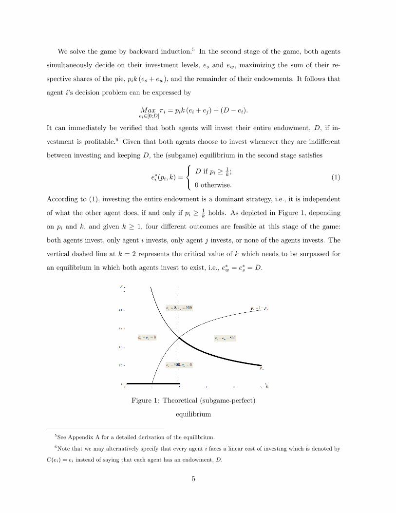
We solve the game by backward induction.5 In the second stage of the game, both agents

simultaneously decide on their investment levels, es and ew, maximizing the sum of their re-

spective shares of the pie, pik (es + ew), and the remainder of their endowments. It follows that

agent i�s decision problem can be expressed by

Maxei2[0;D]

�i = pik (ei + ej) + (D � ei).

It can immediately be veri�ed that both agents will invest their entire endowment, D, if in-

vestment is pro�table.6 Given that both agents choose to invest whenever they are indi¤erent

between investing and keeping D, the (subgame) equilibrium in the second stage satis�es

e�i (pi; k) =

8<: D if pi � 1k ;

0 otherwise.(1)

According to (1), investing the entire endowment is a dominant strategy, i.e., it is independent

of what the other agent does, if and only if pi � 1k holds. As depicted in Figure 1, depending

on pi and k, and given k � 1, four di¤erent outcomes are feasible at this stage of the game:

both agents invest, only agent i invests, only agent j invests, or none of the agents invests. The

vertical dashed line at k = 2 represents the critical value of k which needs to be surpassed for

an equilibrium in which both agents invest to exist, i.e., e�w = e�s = D.

Figure 1: Theoretical (subgame-perfect)

equilibrium

5See Appendix A for a detailed derivation of the equilibrium.

6Note that we may alternatively specify that every agent i faces a linear cost of investing which is denoted by

C(ei) = ei instead of saying that each agent has an endowment, D.

5

In the �rst stage of the game, agent s decides on how much of k (es + ew) to concede to w

by choosing pi. It is straightforward to see that s has a strict incentive to induce w to invest

whenever k � 2. Since she is a dictator at this stage of the game and her pro�t is strictly

decreasing in pw and strictly increasing in ps, respectively, agent s will choose a share such that

w is just indi¤erent between investing D or keeping D. It follows that s�s optimal choice is given

by

p�w(k) =

8<:1k if k � 2;

0 otherwise,(2)

with p�s(k) = 1� p�w(k). In equilibrium, given k � 2, both agents invest their entire endowment

and their pro�ts are �w = 2D and �s = 2(k � 1)kD. If, however, k < 2 holds, then only s

invests and keeps the entire pro�t for herself, i.e., p�w = 0. Thereby, agent w realizes �w = D,

while agent s�s pro�t is �s = kD. We depict the equilibrium share conceded to w, p�w(k), by the

bold black line in Figure 1. In the following sections, this theoretical equilibrium will serve as a

reference.

3 Experimental Design

In our experiment, each subject played 10 rounds of the same treatment. Every round consisted

of two stages. In the �rst stage, the computer randomly assigned a role to each subject after a

random matching. Agent s �rst had to decide on the division of the pie which was generated

in the second stage of the game by both agents investing non-cooperatively and simultaneously.

Each subject received an initial endowment of 500 experimental currency units (ECU, called

�Taler� during the course of the experiment) of which the players could invest any discrete

amount. After investments were chosen, earnings were calculated and information about the

player�s own behavior and the other player�s behavior were given out to the subjects. In addition,

we provided information about players�decisions and earnings in the particular round as well as

the player�s own history of decisions and outcomes of all previous rounds. Then, the next round

started with a new random matching of subjects.

Instructions were kept in a neutral language.7 Agents were labeled �participants�and the

amounts chosen by the subjects in the second stage were called �investments�. Instructions were

7See Appendix B for a transcript of the instructions.

6

distributed prior to the �rst round and read in silence by the participants who could then ask

questions in private. In addition, they had to correctly answer a number of control questions

which addressed the structure of the stages in the game, the decision order for the players, and

the calculation of pro�ts. Once the experimenters had ensured that everyone had understood the

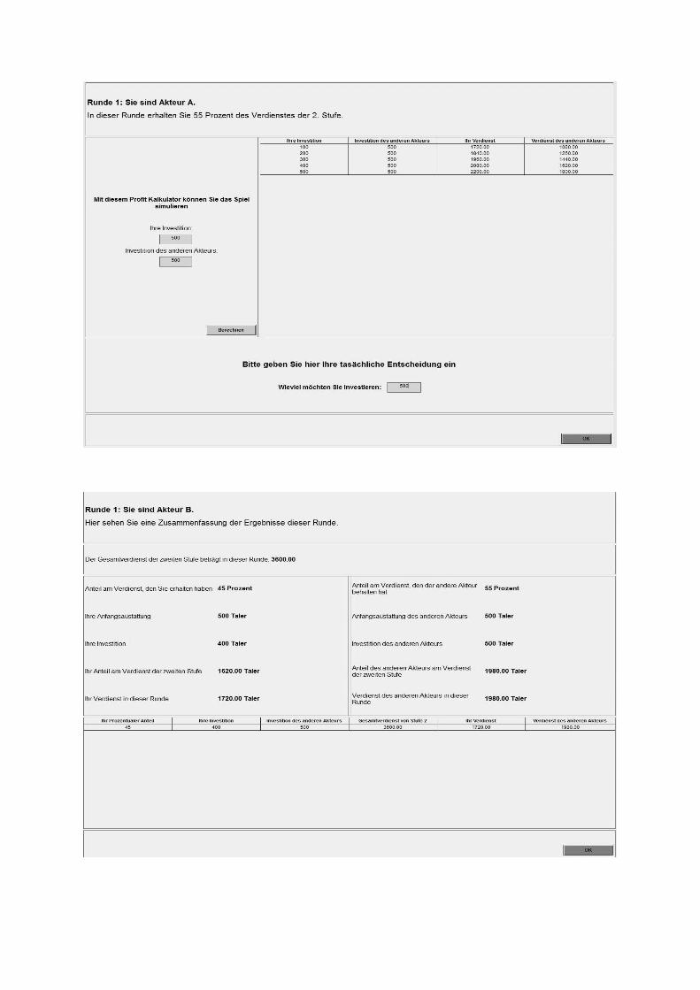
game, the �rst computer screen was displayed and subjects could submit their decisions.8 In each

stage, subjects could use a pro�t calculator for simulation purposes. Therefore, it would have

been possible for any participant to establish rational responses conditional on any expectation

of the other player�s behavior.

After the �nal round, the individual pro�ts of each round were summed up and converted

to payo¤s by a treatment speci�c exchange rate. The exchange rates were chosen to keep the

expected earnings from the treatments similar while still helping to induce a relative distance

between the treatments regarding the weight of the endowment and the size of the pie, respec-

tively. In the �rst treatment, the exchange rate was set to 10 units of the ECU equaling 0:01

e. The size of the pie in the �rst treatment was determined by k = 2:5 times the sum of both

players�investments in the second stage. In the second treatment, the exchange rate was set to

20 units of ECU equaling 0:01 e. Thus, as their nominal value in ECU remained unchanged,

the relative value of the initial endowments was virtually reduced by half between treatments.

Besides, the productivity factor of investments was increased to k = 4. All other things being

equal, we are convinced that this parameter speci�cation induces a higher initial investment

incentive in the second stage.9 Correspondingly, we call the treatment with the smaller (big-

ger) maximum attainable size of the pie and investment incentive, respectively, that is k = 2:5

(k = 4), L-treatment (H-treatment).

The experiments were conducted in the DICE Laboratory for Experimental Economics be-

tween May 2011 and January 2012. Random matching took place in matching groups of eight

subjects each which remained unchanged over the course of a session. Thus, for the econometric

analysis independent observations are given on the matching group level rather than on an indi-

vidual level. We ran eight sessions with 16 subjects in each session, thus totaling 64 subjects per

8See Appendix C for an overview of the computer screens used in the course of the experiment.

9Notice that both in terms of nominal values and real values the investment incentive, i.e., the marginal gain

of investing, is strictly larger for k = 4 given pi > 0 and pj > 0, respectively, with i 6= j.

7

treatment and 80 independent observations in each.10 Subjects were recruited from all faculties

using the Online Recruitment System for Economic Experiments (ORSEE, see Greiner, 2004).

25 percent of the subjects declared to study courses a¢ liated to the Faculty of Business and

Economics.11�12 Forty-one percent of the subjects declared to be female. The experimental

software was developed in z-Tree (see Fischbacher, 2007). One session lasted about 50 minutes

on average. Average earnings were 9:60 e in the L-treatment and 7:61 e in the H-treatment.

In addition to their individual earnings, subjects received an obligatory show-up payment of 4

e.

4 Results

4.1 Theory vs. Experiment

We begin by asking whether our experimental data con�rm the theoretical predictions of our

model in Section 2. Therefore, we formulate the following hypothesis.

Hypothesis 1 (SPE). Agent s �rst chooses p�w = 1=k, and both agents subsequently respond

10The results of a preliminary session with 18 subjects conducted on May 17, 2011, were dropped as a pre-

cautionary measure. Matching groups in this session contained six subjects only. Participants would therefore,

though told otherwise in the instructions, have encountered the same subject twice on average during the course

of the experiment. Such a setting might be too prone to potential reputation e¤ects. Hence, we neglected the

results from this session for the following descriptions and estimations.

11That is, they declared in a non-incentivized standard questionnaire that they were students of either the

B.Sc. or M.Sc. programs in Economics, Business Administration or Business Chemistry. Some of the subjects

did not answer these questions as completing the questionnaire was not compulsory. Therefore, the number has

to be regarded as a lower bound for the actual fraction of economists in the room. An upper bound for the actual

fraction of economists in the experiment might be 37.5 percent as 62.5 percent of the participants declared that

they studied courses in faculties other than the Faculty of Business and Economics.

12Fehr et al. (2006) and Engelmann and Strobel (2006) discuss whether economics majors may behave di¤erently

in simple distribution experiments. We decided to include economics students into the subject pool. This approach

is appropriate since (a) the majority of students in the pool consisted of undergraduates (who might not yet be

in�uenced by strategic thinking in the same way as graduate students are), and (b) we �nd eliminating economics

students from experiments is overly arti�cial and biasing in itself because a reasonable part of social interaction

in reality is in�uenced by explicit economic thinking and economic education.

8

by setting e�i (pi; k) =

8<: D if pi � 1k ;

0 otherwise., with i = s; w.

If the conditions of a subgame perfect equilibrium (SPE) are met, agent s should concede

just as much as to make agent w indi¤erent between investing and keeping D. The equilibrium

shares are 40 percent and 25 percent in the L-treatment and in the H-treatment, respectively.

Then, both agents should always invest 500 ECU. Thereby, s would earn 1; 500 ECU (3; 000

ECU), while w would earn 1; 000 ECU (1; 000 ECU) in the L-treatment (H-treatment).

Recall that our observations are given on the matching group level. We present some de-

scriptive statistics in Table 1.

variable mean std. dev. min max

L-treatment

pw .2934 .1413 .025 .65

es 420.3125 85.2335 190 500

ew 192.7375 125.515 0 500

H-treatment

pw .2567 .0991 .065 .49

es 474.6156 43.8024 337.5 500

ew 206.1406 123.2065 0 500

Table 1: Descriptive statistics per matching group

In the L-treatment, the mean share conceded to w is :2934 and is thus well below the optimal

o¤er, p�w(L) = :4, predicted by the theoretical equilibrium. In the H-treatment, the theoretical

optimum is almost reached, though only on average. The average share conceded by s is :2567,

and is thus close to the optimal proposal of p�w(H) = :25. This observation is con�rmed by

a t-test to check for statistically signi�cant di¤erences between our experimental data and the

theoretical predictions. The p-values are :00 and :5461 for the L-treatment and the H-treatment,

respectively.13 Thus, we �nd evidence that the predicted equilibrium share is chosen on average

13The t-test may only be applied if the respective variables follow a normal distribution. For the shares chosen

by the strong agents a normality test shows that the null hypothesis cannot be rejected.

9

in the H-treatment, whereas the average share falls short of the equilibrium values in the L-

treatment. Figure 2 depicts the sorted average shares per treatment, pw(m), with m = L;H.

Figure 2: Average splitting decisions per

matching group

While the average shares conceded to agent w in the H-treatment oscillate near their corre-

sponding theoretical optimum, indicated by the dashed grey line, the average shares in the

L-treatment are almost constantly below the theoretical prediction, p�w(L) = :4, given by the

dashed black line.

We have controlled for possible learning e¤ects over the course of the experiment by compar-

ing clusters of earlier rounds to those of later rounds both on the average matching group level

and on the individual matching group level. Wilcoxon signed-rank tests reveal no signi�cant

di¤erences between clusters in the H-treatment, whereas statistically signi�cant di¤erences are

found for the L-treatment.14 The persistence of these �ndings for the L-treatment over time,

however, indicates a negative trend rather than initial learning. Hence, in both treatments the

elimination of �rst and/or last round data is not appropriate.

Strong agents invested more on average than weak agents. Weak agents invested ew(L) =

192:74 ECU and ew(H) = 206:14 ECU in the L-treatment and in the H-treatment, respectively,

where the upper bar indicates the average values. Strong agents invested es(L) = 420:31 ECU

14For this decision pattern mental accounting on behalf of the constrained dictators may be responsible. In

particular, we cannot reject that the subjects� propensity to propose riskier, that is lower shares, which put

investments by weak agents at danger, does not increase in the sum of earnings from past periods.

10

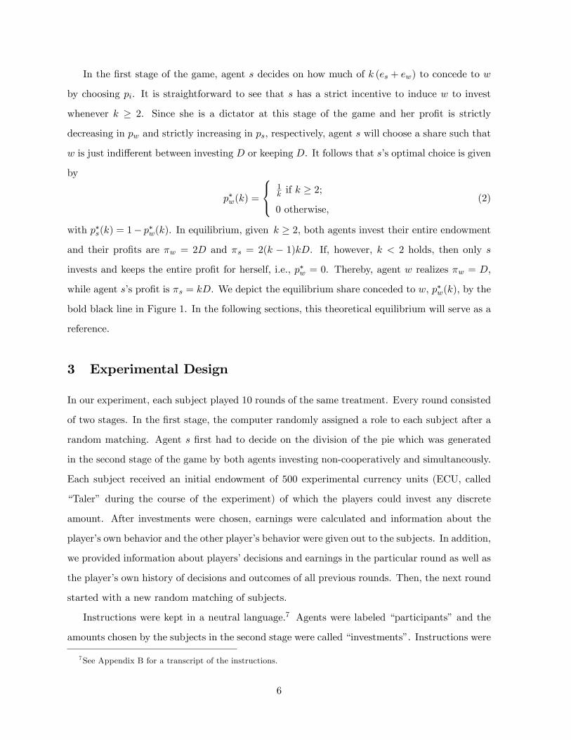
and es(H) = 474:62 ECU in the respective treatments. Recall that equilibrium investments

would have implied that all agents invest their entire endowments in both treatments given

optimal division, p�w(m). However, from our analysis of the decisions on pw, we know that pw

has not been chosen optimally in the L-treatment, whereas the average share comes close to the

optimal value in the H-treatment. Therefore, we need to examine the theoretical best responses

for each agent and for each treatment, given the divisions from stage one, and compare them

to the investment decisions taken in the lab. It is straightforward that the theoretical best

responses do not simply state that both agents should invest 500 ECU in both treatments. This

is illustrated by the following �gures in which both agents�theoretical best responses for each

matching group, e�w and e�s, and average investment decisions for each matching group, ew and

es, are depicted by the dashed lines and by the solid lines, respectively. Figure 3 (a) represents

the L-treatment and �gure 3 (b) represents the H-treatment. Note that the black lines depict

agent s, while the grey lines depict agent w.

Figure 3: (a) Average investment decisions per matching group in the L-treatment; (b)

Average investment decisions per matching group in the H-treatment

It can immediately be seen that both agents invest well below their optimal values in both treat-

ments most of the time. This observation is further con�rmed by a Kolmogorov-Smirnov test

on the equality of the average investment decisions in the lab and the corresponding theoretical

best responses. Both agents invest signi�cantly less than they should from a theoretical point

of view (given pw from stage one).

11

Though our �ndings suggest that the theoretical model is not particularly well-suited to pre-

dict the observed behavior in the lab, we show that at least the relationship between investments,

es and ew; and shares, pw (ps), is as the theory predicts. Table 2 presents Spearman�s rank cor-

relation coe¢ cients for the constrained dictators�proposals in stage one and the corresponding

investment decisions in stage two.

L-treatment H-treatment

pw and ew pw and es pw and ew pw and es

Spearman�s rho 0:7312��� �0:4498��� 0:7544��� �0:0991

Table 2: Spearman�s rank correlation coe¢ cient test

We �nd that ew and pw are signi�cantly correlated with a positive sign. Though negative

(�0:3810 in the L-treatment and �0:0714 in the H-treatment), thus pointing in the presumed

direction, the correlation between agent s�s investment decision, es, and the share of the pie

conceded to w, pw, is only signi�cant in the L-treatment. This result must, however, be seen

with caution. Since, in most of the cases, pw is chosen such that it is pro�table for s to invest, we

rarely observe a su¢ ciently high pw to explain (from a theoretical point of view, at least) why

agent s would refrain from investing D. The same problem prevails in terms of causality. We

ran �xed e¤ects panel regressions, in which we controlled for unobserved heterogeneity between

the matching groups to check whether the level of pw explained the investment decisions taken

by both agents. We report the results in the following table.

Agent s Agent w

L-treatment H-treatment L-treatment H-treatment

coe¤. std. err. coe¤. std. err. coe¤. std. err. coe¤. std. err.

pw -2.728��� .718 -.422 .554 5.6��� .912 7.679��� 1.002

const. 500.351��� 22.427 485.456��� 15.012 28.421 28.473 9.017 27.128

Table 3: Panel regression (�xed e¤ects) on individual (group) level

Whereas agent w�s investment choice is signi�cantly and positively a¤ected by her pro�t-

share, pw, in both treatments, the result for agent s is ambiguous. In the L-treatment, pw exerts

a signi�cantly negative e¤ect on es. However, in the H-treatment, the coe¢ cient is negative, but

12

insigni�cant. Again, we claim that this result is explained by the small number of observations

on pw which suggests that agent s should not invest, rather than by the absence of a signi�cantly

negative relationship between es and pw.

4.2 Varying Investment Incentives

We analyze whether the participants�behavior di¤ers across treatments to check for treatment

e¤ects. It is important to note that we interpret di¤erences in k as indicative of varying invest-

ment incentives. That is, we resort to the common understanding that, all other things being

equal, a higher maximum attainable size of the pie generally increases the agents�incentives to

invest.

In theory, both treatments di¤er substantially, as optimal division, p�w(m), is :25 in the H-

treatment and :40 in the L-treatment. From that we derive Hypothesis 2, by which we postulate

higher values of pw(m) for the treatment with lower investment incentives.

Hypothesis 2. Lower investment incentives lead to larger proposals by the constrained

dictators, i.e., pw(L) > pw(H) holds on average per matching group.

From Figure 2 the validity of Hypothesis 2 could be expected. At least with respect to

those �ve matching group clusters with the highest average proposals on the right, it is obvious

that proposals in the L-treatment are greater than those in the H-treatment. However, this

impression is not unambiguously con�rmed by statistical tests. A Wilcoxon rank-sum (Mann-

Whitney) test returns a p-value of :1024. That is, with respect to the share of the pie conceded

to w, pw, the identity of both treatments may be, though with caution, rejected.

Next, we ask whether there is any treatment e¤ect on both agents� investment decisions.

From theory we would not expect a treatment e¤ect; in either treatment, strong agents decide

on the division of the pie such that incentives for strong and weak agents to fully invest are

provided. Therefore, we derive Hypothesis 3.

Hypothesis 3. There is no treatment e¤ect on investment decisions, i.e., ew(L) = ew(H)

and es(L) = es(H) hold on average per matching group.

We performed Wilcoxon rank-sum (Mann-Whitney) tests to check for possible di¤erences

between investment decisions. With respect to the strong agents�investment decisions identity

13

in the L-treatment and in the H-treatment may be rejected (p-value: :00), whereas it may

not be rejected with respect to the weak agents�decisions (p-value: :6132).15 That is, we �nd

statistical evidence of a clear treatment e¤ect on strong agents�investment behavior, but none

with respect to weak agents�investment behavior. On average, strong agents invested less when

investment incentives were low, i.e., k = 2:5. This treatment e¤ect is illustrated in Figure 4,

in which black dots and diamonds depict the matching group average investment decisions by

strong agents and grey dots and diamonds show those taken by the weak agents.16

Figure 4: The impact of varying investment

incentives on average investment decisions per

matching group

We turn to the size of the pie and welfare as measures for team productivity and e¢ ciency,

respectively. Pie size, Cg;t (m) = k (es;g;t + ew;g;t), determines team productivity for each match-

ing group g = 1; :::; 8 in period t = 1; :::; 10. When both agents fully invest, then the pie size

takes on the values 2; 500 and 4; 000 in the L-treatment and in the H-treatment, respectively.

It is straightforward that the treatments cannot be compared in terms of absolute values. We

therefore focus on relative pie size deviations from their theoretical benchmarks. We use the

15Alternatively, one could use the Kolmogorov-Smirnov test to check for treatment e¤ects on the agents� in-

vestment behavior and on the constrained dictators�splitting decisions. The results con�rm our �ndings based

on the Wilcoxon rank-sum (Mann-Whitney) test.

16For the sake of comparison, in Figure 4, Figure 5, and in Figure 6 matching groups are sorted by the extent

of the average deviation from the optimum.

14

measure eCg;t (m) = Cg;t (m)

C (m)�, (3)

where C (m)� is the (optimum) productivity level, with m = H;L, predicted by our theoretical

benchmark. Cg;t (m) denotes the pie size realized in period t by matching group i in treatment

m. eCg;t (m) is equal to one if matching group g�s team productivity at time t corresponds to thetheoretical optimum and is less than one if it is below optimum. It can immediately be veri�ed

that the higher (3), the lower the (negative) deviation from optimal pie size, C (m)�.

Pie size is always maximized in the theoretical optimum of our model regardless of the agents�

actual investment incentives. Therefore, we derive Hypothesis 4.

Hypothesis 4. There is no treatment e¤ect regarding team productivity. That is, normalized

pie sizes are equal in the L-treatment and in the H-treatment, i.e., eCg;t (L) = eCg;t (H) holds.In Figure 5, we provide the average relative pie size deviations per matching group for both

treatments. Instead of accounting for each period, t, we use average deviations per matching

group, Cg(m), which are calculated using Cg(m) =PteCg;t(m)=10.

Figure 5: The impact of varying investment

incentives on the average pie size per matching

group

Figure 5 shows that average deviations are higher when investment incentives are low. The

black line, which depicts average deviations per matching group in the L-treatment, is constantly

below the grey line, which depicts the average deviations per matching group in theH-treatment.

15

This observation seems a plausible consequence of the constrained dictators�investment behavior

in the lab; they invest less when investment incentives are low, while recipients�investments are

identical on average across treatments. The observation is con�rmed by a Wilcoxon rank-sum

(Mann-Whitney) test. The identity of average deviations, eCg;t (m), in the L-treatment and inthe H-treatment has to be rejected (p-value: :0017). Thus, in our setting lower investment

incentives have a detrimental e¤ect on team productivity.

We have to treat the results with caution, as a similar analysis may be performed with respect

to averaged welfare, W g(m), which is derived from the pie size plus the respective remainder of

the endowments. As before, we make use of the normalized welfare measure

fWg;t (m) =Wg;t (m)

W (m)�. (4)

Wg;t (m) is the agents�(partial) welfare for each matching group, g = 1; :::; 8; and period,

t = 1; :::; 10. W (m)� is welfare in the theoretical benchmark for treatment m, with m = L;H.fWg;t (m) is equal to one if matching group g�s welfare at time t corresponds to the theoretical

optimum and is less than one if welfare is below optimum. In the theoretical benchmark, welfare

and pie size are equal, since both agents fully invest regardless of k. Because of the latter, again,

we do not expect di¤erences between treatments. We may therefore state Hypothesis 5 in

analogy to Hypothesis 4.

Hypothesis 5. There is no treatment e¤ect regarding welfare. That is, normalized welfare

is equal in the L-treatment and in the H-treatment, i.e., fWg;t (L) = fWg;t (H) holds.

Again, we inspect some descriptive statistics to compare the treatments. Figure 6 o¤ers an

illustration of the average welfare deviations per matching group, W g (m), which are calculated

by W g (m) =PtfWg;t (m) =10.

For the four matching groups with the highest deviations (matching groups 1-4 on the left

in Figure 6) the averaged normalized welfare deviation is lower when investment incentives are

low, as the black line for the L-treatment is running above the grey line for the H-treatment.

For the four matching groups with lowest deviations (matching groups 5-8 on the right in Figure

6) the ordering is reversed. Here, lower investment incentives induce lower averaged normalized

welfare deviations. A Wilcoxon rank-sum (Mann-Whitney) test con�rms this impression so that

16

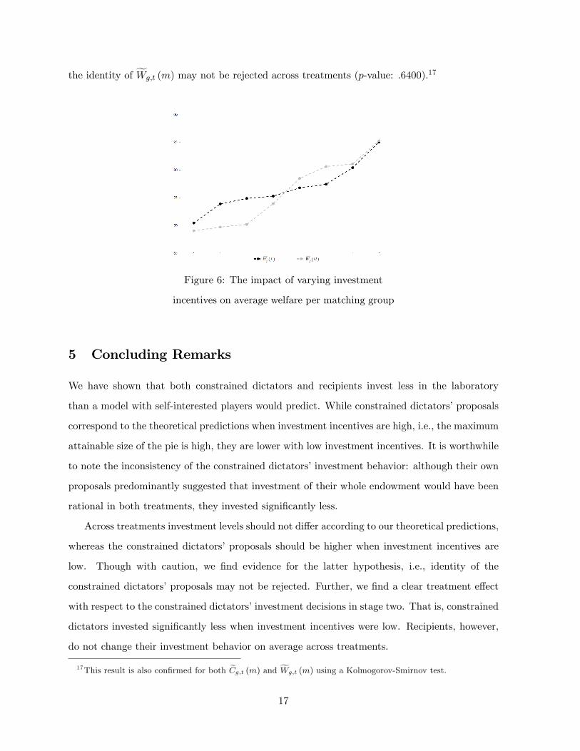
the identity of fWg;t (m) may not be rejected across treatments (p-value: :6400).17

Figure 6: The impact of varying investment

incentives on average welfare per matching group

5 Concluding Remarks

We have shown that both constrained dictators and recipients invest less in the laboratory

than a model with self-interested players would predict. While constrained dictators�proposals

correspond to the theoretical predictions when investment incentives are high, i.e., the maximum

attainable size of the pie is high, they are lower with low investment incentives. It is worthwhile

to note the inconsistency of the constrained dictators�investment behavior: although their own

proposals predominantly suggested that investment of their whole endowment would have been

rational in both treatments, they invested signi�cantly less.

Across treatments investment levels should not di¤er according to our theoretical predictions,

whereas the constrained dictators�proposals should be higher when investment incentives are

low. Though with caution, we �nd evidence for the latter hypothesis, i.e., identity of the

constrained dictators�proposals may not be rejected. Further, we �nd a clear treatment e¤ect

with respect to the constrained dictators�investment decisions in stage two. That is, constrained

dictators invested signi�cantly less when investment incentives were low. Recipients, however,

do not change their investment behavior on average across treatments.

17This result is also con�rmed for both eCg;t (m) and fWg;t (m) using a Kolmogorov-Smirnov test.

17

Finally, we asked whether increasing the maximum attainable size of the pie and, thereby,

investment incentives have an impact on team productivity and welfare. Instead of using absolute

values for both team productivity and welfare, we computed relative measures of deviation from

the theoretical optima. On the one hand, we �nd evidence that team productivity is higher when

investment incentives are high. On the other hand, we do not �nd that varying the investment

incentives makes a statistically signi�cant di¤erence in terms of welfare. This is easily explained

when one keeps in mind that welfare, in contrast to team productivity, accounts for the players�

residual endowment and, thereby, for the amount of money not invested.

Only one part of our results may be explained by the characteristics we have deliberately

chosen in the experiment. While nominal parameter and outcome settings di¤ered by obvious

margins, we have also used di¤erent exchange rates, which make treatments similar in real

terms. In the low investment incentives treatment, endowments were 0:50 e per agent and per

round, whereas they were just 0:25 e per agent and per round in the high investment incentives

treatment.18 Show-up fees amounted to a real value of 4 e in both treatments, while maximum

attainable pie sizes were 2:50 e in the L-treatment and 2 e in the H-treatment. Focusing

on the theoretical optimum though, di¤erences between treatments are not obvious when real

values rather than nominal values are considered. More speci�cally, suppose that the constrained

dictator chose the equilibrium o¤er, p�w(k), and both agents responded accordingly by investing

their whole endowments, then the constrained dictators would have earned 1:50 e in real terms

irrespective of the treatment. However, a strictly larger incentive to invest is preserved in the

high investment incentive treatment, since the marginal gain from investing is, all other things

being equal, higher regardless of the di¤erences between nominal and real values.

We are convinced that the constrained dictator game covers various examples of economic

actions. For instance, our setup is well suited to examine the e¤ects of so-called occupational

unions in labor con�icts. Recall that, in contrast to trade unions and industrial unions, occu-

pational unions are job-speci�c and typically represent the interests of those parts of a �rm�s

workforce which are characterized by high skill levels and sit in pivotal positions of the pro-

duction process. As they are not easy to be substituted, they own strong bargaining power

18This di¤erence between endowments in real terms could constitute an endowment e¤ect, which might also

explain one part of the subjects�behavior in the lab (see Kahneman et al. (1990)).

18

relative to other worker groups. In Germany, for instance, major examples are the unions of

train drivers, civil aviation pilots, and hospital physicians. In our setup, the occupational union

would be represented by the constrained dictator. Though the occupational union could fully

appropriate a �rm�s available rent for her members through higher wages, it will crucially depend

on the remaining workforce�s action, since the appropriable rent is a team product rather than

the consequence of a sole action by one part of the workforce. Hence, the crucial question is

whether or not occupational unions would make excessive use of their bargaining power, so that

the team�s productivity is negatively a¤ected. As a further example may serve R&D coopera-

tions of a dominant organization and a minor �rm, in which the former might have the power to

appropriate the whole joint surplus generated by R&D in the product market. Nonetheless, the

surplus would be positively a¤ected by the small �rm�s behavior, since the R&D cooperation

would yield maximum results only if both �rms fully contribute. Finally, the typical principal

agent problems in small- and medium-sized owner-led enterprises may serve as an example. The

owner of the �rm is not only the administrator of the business, but is also involved in the pro-

duction of the �rm�s �nal team product. Thus, such an owner would also be a dictator limited

by her employees�behavior, i.e., she is a constrained dictator.

19

Appendix A

Theoretical Prediction. It is straightforward to see that �i is linear and monotone in ei,

i.e., @�i=@ei 6= 0 if pi 6= 1=k and @2�i=@e2i = 0. More precisely, �i is monotonically increasing

(decreasing) in ei if pi > 1=k (pi < 1=k). This is true irrespective of the other agent�s decision,

ej , with j 6= i. Hence, depending on pi, it is optimal for agent i either to invest her entire

endowment, D, or not to invest at all, i.e., ei = 0. Note that each agent�s decision is a discrete

(binary) choice due to �i�s properties, although ei is a continuous variable. Therefore, the game

may be be reduced to a normal form representation as in Table 4. s is the column player,

whereas w is the row player.

es = D es = 0

ew = D pwk2D ; psk2D pwkD ; D + pskD

ew = 0 D + pwkD ; pskD D ; D

Table 4: The agents�investment choice in stage two

It can be immediately inferred that it is each agent�s dominant strategy to invest D if

pi � 1=k and to keep the entire endowment, i.e., ei = 0, if pi < 1=k. This is re�ected by

(1). Thus, the second stage equilibrium decisions, (e�w; e�s), are: (0; D) if pw < 1=k, (D;D) if

1=k � pw � (k � 1)=k, and (D; 0) if pw > (k � 1)=k.

In the �rst stage, agent s decides on how to split k(ew + es) between herself and agent w

maximizing �s = psk(e�s + e�w) + (D � e�s). It is important to note that s acts as a constrained

dictator at this stage of the game: although she has all the bargaining power to decide on pw

and ps, respectively, the size of the pie, k(ew + es), also depends on the weak agent�s decision.

It is never rational for s to keep the entire pie for herself if k � 2. Rather, it is optimal to

set pw = 1=k which triggers w to invest assuming that she prefers investing whenever she is

indi¤erent between investing and keeping D, i.e., pw = 1=k holds.

Appendix B

[Insert Transscript of Instructions here]

20

Appendix C

[Insert Screenshots here]

21

References

[1] Berg, J., Dickhaut, J., and McCabe, K. (1995), Trust, Reciprocity, and Social History,

Games and Economic Behavior 10, 122-142.

[2] Bolton, G. E., and Zwick, R. (1995), Anonymity versus Punishment in Ultimatum Games,

Games and Economic Behavior 10, 95-121.

[3] Cherry, T. L., Frykblom, P., and Shorgen, J. F. (2002), Hardnose the Dictator, American

Economic Review 92, 1218-1221.

[4] Engelmann, D., and Strobel, M. (2006), Inequality Aversion, E¢ ciency and Maximin Pref-

erences in Simple Distribution Experiments: Reply, American Economic Review 96, 1918-

1923.

[5] Fehr, E., Naef, M., and Schmidt, K. M. (2006), Inequality Aversion, E¢ ciency and Maximin

Preferences in Simple Distribution Experiments: Comment, American Economic Review 96,

1912-1917.

[6] Fischbacher, U. (2007), z-Tree �Zurich Toolbox for Readymade Economic Experiments,

Experimental Economics 10, 171-178.

[7] Forsythe R., Horowitz, J. L., Savin, N. E., and Sefton, M. (1994), Fairness in Simple

Bargaining Experiments, Games and Economic Behavior 6, 347-369.

[8] Greiner, B. (2004), An Online Recruitment System for Economic Experiments, in: K. Kre-

mer and V. Macho, eds. Forschung und wissenschaftliches Rechnen 2003, GWDG Bericht

63, Gesellschaft wir wissenschaftliche Datenverarbeitung, Göttingen, Germany, 79-83.

[9] Heinz, M., Juranek, S., and Rau, H. (2012), Do Women Behave More Reciprocally than

Men? Gender Di¤erences in Real E¤ort Dictator Games, Journal of Economic Behavior

and Organization 83, 105-110.

[10] Ho¤man, E., McCabe, K., Shachat, K., and Smith, V. (1994), Preferences, Property Rights,

and Anonymity in Bargaining Games, Games and Economic Behavior 7, 346-380.

22

[11] Ho¤man, E., McCabe, K., and Smith, V. (1996), Preferences, Property Rights, and

Anonymity in Bargaining Games, American Economic Review 86, 653-660.

[12] Kahneman, D., Knetsch, J. L., and Thaler, R. H. (1986), Fairness and the Assumptions of

Economics, Journal of Business 59, 285-300.

[13] Kahneman, D., Knetsch, J. L., and Thaler, R. H. (1990), Experimental Tests of the En-

dowment E¤ect and the Coase Theorem, Journal of Political Economy 98, 1325-1348.

[14] Konow, J. (2000), Fair Shares: Accountability and Cognitive Dissonance in Allocation

Decisions, American Economic Review 90, 1072-1091.

[15] Oxoby, R. J., and Spraggon, J. (2008), Mine and Yours: Property Rights in Dictator Games,

Journal of Economic Behavior and Organization 65, 703-713.

[16] Ru­ e, J. B. (1998), More Is Better, But Fair is Fair: Tipping in Dictator and Ultimatum

Games, Games and Economic Behavior 23, 247-265.

[17] Van Huyck, J. B., Battalio, R. C., andWalters, M. F. (1995), Commitment versus Discretion

in the Peasant-Dictator Game, Games and Economic Behavior 10, 143-170.

23

Transcript of L-Treatment Instructions

Welcome to this decision experiment!

Basic Information

Please read these instructions very carefully! At the end of these instructions you will find some

control questions. The control questions will give you and the experimenters the final chance to check

whether you have fully understood the rules of the experiment. Your decisions during the control

questions will have no effect on your earnings from the experiment.

After you have answered the control questions correctly the experiment will start.

During the experiment you will make decisions by which you can earn money. How much money you

will earn depends on the decisions you take and on the decisions the other participants take. ECU is

the currency used during the experiment.1 At the end of the experiment, the amount of ECU earned

will be converted to Euro according to an exchange rate of

10 ECU = 1 Cent.

Your earnings will then be paid to you. In addition to your earnings from the experiment, you will

receive a secure show-up payment of 4 EUR.

You will start the experiment with an initial endowment of 500 ECU (50 cents). This amount will be

increased by your earnings and decreased by your losses. You may always exclude losses by your own

decisions.

After the experiment has been concluded, the sum of your earnings in the rounds will be converted

into Euro and paid to you. That is, every decision you take will affect your payment. In addition to

your earnings you will get a decision independent payment of 4 € (show-up payment). Apart from the

experimenters no one else will get to know your earnings from the experiment and the amount of

money that is paid to you.

The experiment takes place anonymously, that is, you will not know which of the other participants

you are interacting with.

Please note that you are not allowed to talk to any other participant throughout the experiment! Should

this happen, we will be forced to abandon the experiment. If you have any question, please hold your

hand up and an experimenter will come to you!

Course of the Experiment

Decision Structure

In the experiment an agent “A” encounters an agent “B”. Each round of the experiment consists of two

stages. In the first stage agent A decides on how the earnings from the subsequent second stage will be

1 In German the expression “Taler” was used instead of Experimental Currency Unit (ECU).

divided between himself and agent B. In the second stage agent A and agent B choose simultaneously

and independently which amount of ECU they want to invest.

At the beginning of each round it will be randomly determined whether you are an agent of type A or

type B. Your type will then be displayed on top of the screen.

The experiment will last for 10 rounds. In each round, pairings will be drawn, each consisting of an

agent A and an agent B. For each new round a new pairing will be randomly drawn. Information about

your decisions and your performance will only be communicated to the respective other agent in that

round. All the other agents will not learn anything about your choices!

In the following, we explain choice alternatives and their consequences for the respective agent’s

earnings.

Stage 1

In the first stage agent A decides on how the earnings from the subsequent second stage will be

divided between himself and agent B. To do so agent A has to choose an integer value from 0 to 100,

indicating the share of the total earnings obtained in the second stage which he will concede to agent

B.

If he chooses 20, for instance, 20 percent of the earnings in the second stage are left with agent B, if he

chooses 63, for instance, then 63 percent of the earnings in the second stage are left with agent B.

Agent A has an on-screen calculator at his disposal. He can enter his own planned investment, the

expected second stage investment by agent B, and proposals for the division of the total earnings to be

decided by himself in the first stage. The on-screen calculator then determines the earnings for both

agents from the proposed decisions.

The on-screen calculator returns information on the division entered, the investments entered, and the

earnings resulting from these inputs. The information on earnings is differentiated into earnings from

investment and division in the second stage and total earnings for each agent, which also includes the

residuum of the initial endowment.

The earnings in the second stage, which will be split between the agents, will be calculated as follows:

A B2.5 i i . Ai refers to the amount of investment of agent A and Bi is the investment of agent B.

Thus, the sum of the investments by both agents will be multiplied by 2.5 in order to determine their

earnings from investment in the second stage.

Stage 2

In the second stage agent B finds out about agent A’s decision in the first stage.

Subsequently, agent A and agent B invest an amount of money simultaneously and independently.

That is, they do not know of the investment decision of the respective other. In each round, each of the

agents has a maximum of 500 ECU (50 cents) at his disposal. Everyone may therefore invest an

integer value from 0 to 500 ECU. Residual money which has not been invested may be kept by the

agent. In particular this means that the total earnings of an agent who invests 0 ECU is 500 ECU (50

cents).

Apart from their investments, agents do not have to bear any costs.

Again, both agents have an on-screen-calculator at their disposal for informative purposes. Subjects

may enter their own planned investment and the expected investment of the other agent. The on-screen

calculator then determines the expected earnings for both agents while taking the decision on the

division from the first stage into account. The on-screen calculator returns information on the

investment decisions entered and the resulting earnings for the agents, both as earnings from the

investment in the second stage and as total earnings including the residuum of the initial endowment.

At the end of each round, the agents will also be fully informed about the actual decisions taken. On

the screen they will get information on the division agent A has chosen in the first stage and the

investment decisions of agent A and agent B in the second stage. In accordance to the division and

investments, the earnings of the agents will be calculated and displayed.

Example

Agent A decides to concede, for instance, 15 percent of the earnings from the second stage of the

experiment to agent B, thus keeping 85 percent for himself. If both invest 100 ECU of their initial

endowment, agent A yields (2.5 * (100 + 100) * 0.85) as earnings from the second stage, that is 425

ECU, and agent B yields 75 ECU. Adding their retained initial endowments agent A would therefore

yield total earnings of 825 ECU in this round of the experiment and agent B 475 ECU.

After reading and confirming the displayed information on the results the next round of the experiment

is going to commence.

Conclusion and Payment

After 10 rounds the experiment ends. Before making the pay-outs we will ask you to answer a final

questionnaire. Your answers to the final questionnaire will not have any effect on your payments.

Please press the confirm-button after you have completed the questionnaire!

When the experiment is concluded, the Euro-equivalent of the sum of your earnings over the rounds of

the experiment will be paid to you. 10 ECU are equal to 1 cent. In addition to your earnings you will

get a decision independent payoff of 4 € (show-up payment).

Please wait in your cabin until you are called by the experimenters to come forward and collect

your payment! Please hand back all the documentation you have received! Apart from the

experimenters you will be the only one to know your earnings from the experiment and the

amount of money that is paid to you.

Transcript of L-Treatment Control Questions

Question 1: Please tick the correct conclusions! Multiple correct conclusions are possible.

(a) agent A decides in stage 1 first, which proportion of the earnings from stage 2 agent B will

get, and then decides over his investment in stage 2

(b) agent B decides in stage 1 first, which proportion of the earnings from stage 2 agent A will

get, and then decides over his investment in stage 2

(c) only agent B invests in stage 2

(d) only agent A invests in stage 2

(e) both agents invest in stage 2

(f) agent B does not take a decision in stage 1

Question 2: Assume that agent A has set 25 as the share to be conceded to agent B. Earnings of the

second stage are 1,000 ECU, with both agents A and B having invested 200 ECU of their initial

endowments each.

(a) How many ECU does agent A get from the earnings of the second stage?

(b) How many ECU does agent B get from the earnings of the second stage?

(c) What are the total earnings (that is, share of the earning of the second stage + remainder of the

initial endowment) of agent A?

(d) What are the total earnings (that is, share of the earning of the second stage + remainder of the

initial endowment) of agent B?

Question 3: Assume that agent A has set 60 as the share to be conceded to agent B. Earnings of the

second stage are 1,000 ECU, with agent A having invested 300 ECU and agent B having invested 100

ECU of their initial endowments.

(a) How many ECU does agent A get from the earnings of the second stage?

(b) How many ECU does agent B get from the earnings of the second stage?

(c) What are the total earnings (that is, share of the earning of the second stage + remainder of the

initial endowment) of agent A?

(d) What are the total earnings (that is, share of the earning of the second stage + remainder of the

initial endowment) of agent B?

Thank you!

Transcript of H-Treatment Instructions

Welcome to this decision experiment!

Basic Information

Please read these instructions very carefully! At the end of these instructions you will find some

control questions. The control questions will give you and the experimenters the final chance to check

whether you have fully understood the rules of the experiment. Your decisions during the control

questions will have no effect on your earnings from the experiment.

After you have answered the control questions correctly the experiment will start.

During the experiment you will make decisions by which you can earn money. How much money you

will earn depends on the decisions you take and on the decisions the other participants take. ECU is

the currency used during the experiment.2 At the end of the experiment, the amount of ECU earned

will be converted to Euro according to an exchange rate of

20 ECU = 1 Cent.

Your earnings will then be paid to you. In addition to your earnings from the experiment, you will

receive a secure show-up payment of 4 EUR.

You will start the experiment with an initial endowment of 500 ECU (25 cents). This amount will be

increased by your earnings and decreased by your losses. You may always exclude losses by your own

decisions.

After the experiment has been concluded, the sum of your earnings in the rounds will be converted

into Euro and paid to you. That is, every decision you take will affect your payment. In addition to

your earnings you will get a decision independent payment of 4 € (show-up payment). Apart from the

experimenters no one else will get to know your earnings from the experiment and the amount of

money that is paid to you.

The experiment takes place anonymously, that is, you will not know which of the other participants

you are interacting with.

Please note that you are not allowed to talk to any other participant throughout the experiment! Should

this happen, we will be forced to abandon the experiment. If you have any question, please hold your

hand up and an experimenter will come to you!

Course of the Experiment

Decision Structure

In the experiment an agent “A” encounters an agent “B”. Each round of the experiment consists of two

stages. In the first stage agent A decides on how the earnings from the subsequent second stage will be

2 In German the expression “Taler” was used instead of Experimental Currency Unit (ECU).

divided between himself and agent B. In the second stage agent A and agent B choose simultaneously

and independently which amount of ECU they want to invest.

At the beginning of each round it will be randomly determined whether you are an agent of type A or

type B. Your type will then be displayed on top of the screen.

The experiment will last for 10 rounds. In each round, pairings will be drawn, each consisting of an

agent A and an agent B. For each new round a new pairing will be randomly drawn. Information about

your decisions and your performance will only be communicated to the respective other agent in that

round. All the other agents will not learn anything about your choices!

In the following, we explain choice alternatives and their consequences for the respective agent’s

earnings.

Stage 1

In the first stage agent A decides on how the earnings from the subsequent second stage will be

divided between himself and agent B. To do so agent A has to choose an integer value from 0 to 100,

indicating the share of the total earnings obtained in the second stage which he will concede to agent

B.

If he chooses 20, for instance, 20 percent of the earnings in the second stage are left with agent B, if he

chooses 63, for instance, then 63 percent of the earnings in the second stage are left with agent B.

Agent A has an on-screen calculator at his disposal. He can enter his own planned investment, the

expected second stage investment by agent B, and proposals for the division of the total earnings to be

decided by himself in the first stage. The on-screen calculator then determines the earnings for both

agents from the proposed decisions.

The on-screen calculator returns information on the division entered, the investments entered, and the

earnings resulting from these inputs. The information on earnings is differentiated into earnings from

investment and division in the second stage and total earnings for each agent, which also includes the

residuum of the initial endowment.

The earnings in the second stage, which will be split between the agents, will be calculated as follows:

A B4 i i . Ai refers to the amount of investment of agent A and Bi is the investment of agent B.

Thus, the sum of the investments by both agents will be multiplied by 4 in order to determine their

earnings from investment in the second stage.

Stage 2

In the second stage agent B finds out about agent A’s decision in the first stage.

Subsequently, agent A and agent B invest an amount of money simultaneously and independently.

That is, they do not know of the investment decision of the respective other. In each round, each of the

agents has a maximum of 500 ECU (25 cents) at his disposal. Everyone may therefore invest an

integer value from 0 to 500 ECU. Residual money which has not been invested may be kept by the

agent. In particular this means that the total earnings of an agent who invests 0 ECU is 500 ECU (25

cents).

Apart from their investments, agents do not have to bear any costs.

Again, both agents have an on-screen-calculator at their disposal for informative purposes. Subjects

may enter their own planned investment and the expected investment of the other agent. The on-screen

calculator then determines the expected earnings for both agents while taking the decision on the

division from the first stage into account. The on-screen calculator returns information on the

investment decisions entered and the resulting earnings for the agents, both as earnings from the

investment in the second stage and as total earnings including the residuum of the initial endowment.

At the end of each round, the agents will also be fully informed about the actual decisions taken. On

the screen they will get information on the division agent A has chosen in the first stage and the

investment decisions of agent A and agent B in the second stage. In accordance to the division and

investments, the earnings of the agents will be calculated and displayed.

Example

Agent A decides to concede, for instance, 20 percent of the earnings from the second stage of the

experiment to agent B, thus keeping 80 percent for himself. If both invest 200 ECU of their initial

endowment, agent A yields (4 * (200 + 200) * 0.80) as earnings from the second stage, that is 1,280

ECU, and agent B yields 320 ECU. Adding their retained initial endowments agent A would therefore

yield total earnings of 1,580 ECU in this round of the experiment and agent B 620 ECU.

After reading and confirming the displayed information on the results the next round of the experiment

is going to commence.

Conclusion and Payment

After 10 rounds the experiment ends. Before making the pay-outs we will ask you to answer a final

questionnaire. Your answers to the final questionnaire will not have any effect on your payments.

Please press the confirm-button after you have completed the questionnaire!

When the experiment is concluded, the Euro-equivalent of the sum of your earnings over the rounds of

the experiment will be paid to you. 20 ECU are equal to 1 cent. In addition to your earnings you will

get a decision independent payoff of 4 € (show-up payment).

Please wait in your cabin until you are called by the experimenters to come forward and collect

your payment! Please hand back all the documentation you have received! Apart from the

experimenters you will be the only one to know your earnings from the experiment and the

amount of money that is paid to you.

Transcript of H-Treatment Control Questions

Question 1: Please tick the correct conclusions! Multiple correct conclusions are possible.

(g) agent A decides in stage 1 first, which proportion of the earnings from stage 2 agent B will

get, and then decides over his investment in stage 2

(h) agent B decides in stage 1 first, which proportion of the earnings from stage 2 agent A will

get, and then decides over his investment in stage 2

(i) only agent B invests in stage 2

(j) only agent A invests in stage 2

(k) both agents invest in stage 2

(l) agent B does not take a decision in stage 1

Question 2: Assume that agent A has set 25 as the share to be conceded to agent B. Earnings of the

second stage are 1,600 ECU, with both agents A and B having invested 200 ECU of their initial

endowments each.

(e) How many ECU does agent A get from the earnings of the second stage?

(f) How many ECU does agent B get from the earnings of the second stage?

(g) What are the total earnings (that is, share of the earning of the second stage + remainder of the

initial endowment) of agent A?

(h) What are the total earnings (that is, share of the earning of the second stage + remainder of the

initial endowment) of agent B?

Question 3: Assume that agent A has set 60 as the share to be conceded to agent B. Earnings of the

second stage are 1,600 ECU, with agent A having invested 300 ECU and agent B having invested 100

ECU of their initial endowments.

(e) How many ECU does agent A get from the earnings of the second stage?

(f) How many ECU does agent B get from the earnings of the second stage?

(g) What are the total earnings (that is, share of the earning of the second stage + remainder of the

initial endowment) of agent A?

(h) What are the total earnings (that is, share of the earning of the second stage + remainder of the

initial endowment) of agent B?

Thank you!

PREVIOUS DISCUSSION PAPERS

77 Coenen, Michael and Jovanovic, Dragan, Investment Behavior in a Constrained Dictator Game, November 2012.

76 Gu, Yiquan and Wenzel, Tobias, Strategic Obfuscation and Consumer Protection Policy in Financial Markets: Theory and Experimental Evidence, November 2012.

75 Haucap, Justus, Heimeshoff, Ulrich and Jovanovic, Dragan, Competition in Germany’s Minute Reserve Power Market: An Econometric Analysis, November 2012.

74 Normann, Hans-Theo, Rösch, Jürgen and Schultz, Luis Manuel, Do Buyer Groups Facilitate Collusion?, November 2012.

73 Riener, Gerhard and Wiederhold, Simon, Heterogeneous Treatment Effects in Groups, November 2012.

72 Berlemann, Michael and Haucap, Justus, Which Factors Drive the Decision to Boycott and Opt Out of Research Rankings? A Note, November 2012.

71 Muck, Johannes and Heimeshoff, Ulrich, First Mover Advantages in Mobile Telecommunications: Evidence from OECD Countries, October 2012.

70 Karaçuka, Mehmet, Çatik, A. Nazif and Haucap, Justus, Consumer Choice and Local Network Effects in Mobile Telecommunications in Turkey, October 2012. Forthcoming in: Telecommunications Policy.

69 Clemens, Georg and Rau, Holger A., Rebels without a Clue? Experimental Evidence on Explicit Cartels, October 2012.

68 Regner, Tobias and Riener, Gerhard, Motivational Cherry Picking, September 2012.

67 Fonseca, Miguel A. and Normann, Hans-Theo, Excess Capacity and Pricing in Bertrand-Edgeworth Markets: Experimental Evidence, September 2012. Forthcoming in: Journal of Institutional and Theoretical Economics.

66 Riener, Gerhard and Wiederhold, Simon, Team Building and Hidden Costs of Control, September 2012.

65 Fonseca, Miguel A. and Normann, Hans-Theo, Explicit vs. Tacit Collusion – The Impact of Communication in Oligopoly Experiments, August 2012. Forthcoming in: European Economic Review.

64 Jovanovic, Dragan and Wey, Christian, An Equilibrium Analysis of Efficiency Gains from Mergers, July 2012.

63 Dewenter, Ralf, Jaschinski, Thomas and Kuchinke, Björn A., Hospital Market Concentration and Discrimination of Patients, July 2012.

62 Von Schlippenbach, Vanessa and Teichmann, Isabel, The Strategic Use of Private Quality Standards in Food Supply Chains, May 2012. Forthcoming in: American Journal of Agricultural Economics.

61 Sapi, Geza, Bargaining, Vertical Mergers and Entry, July 2012.

60 Jentzsch, Nicola, Sapi, Geza and Suleymanova, Irina, Targeted Pricing and Customer Data Sharing Among Rivals, July 2012.

59 Lambarraa, Fatima and Riener, Gerhard, On the Norms of Charitable Giving in Islam: A Field Experiment, June 2012.

58 Duso, Tomaso, Gugler, Klaus and Szücs, Florian, An Empirical Assessment of the 2004 EU Merger Policy Reform, June 2012.

57 Dewenter, Ralf and Heimeshoff, Ulrich, More Ads, More Revs? Is there a Media Bias in the Likelihood to be Reviewed?, June 2012.

56 Böckers, Veit, Heimeshoff, Ulrich and Müller Andrea, Pull-Forward Effects in the German Car Scrappage Scheme: A Time Series Approach, June 2012.

55 Kellner, Christian and Riener, Gerhard, The Effect of Ambiguity Aversion on Reward Scheme Choice, June 2012.

54 De Silva, Dakshina G., Kosmopoulou, Georgia, Pagel, Beatrice and Peeters, Ronald, The Impact of Timing on Bidding Behavior in Procurement Auctions of Contracts with Private Costs, June 2012. Forthcoming in: Review of Industrial Organization.

53 Benndorf, Volker and Rau, Holger A., Competition in the Workplace: An Experimental Investigation, May 2012.

52 Haucap, Justus and Klein, Gordon J., How Regulation Affects Network and Service Quality in Related Markets, May 2012. Published in: Economics Letters 117 (2012), pp. 521-524.

51 Dewenter, Ralf and Heimeshoff, Ulrich, Less Pain at the Pump? The Effects of Regulatory Interventions in Retail Gasoline Markets, May 2012.

50 Böckers, Veit and Heimeshoff, Ulrich, The Extent of European Power Markets, April 2012.

49 Barth, Anne-Kathrin and Heimeshoff, Ulrich, How Large is the Magnitude of Fixed-Mobile Call Substitution? - Empirical Evidence from 16 European Countries, April 2012.

48 Herr, Annika and Suppliet, Moritz, Pharmaceutical Prices under Regulation: Tiered Co-payments and Reference Pricing in Germany, April 2012.

47 Haucap, Justus and Müller, Hans Christian, The Effects of Gasoline Price Regulations: Experimental Evidence, April 2012.

46 Stühmeier, Torben, Roaming and Investments in the Mobile Internet Market, March 2012. Published in: Telecommunications Policy, 36 (2012), pp. 595-607.

45 Graf, Julia, The Effects of Rebate Contracts on the Health Care System, March 2012.

44 Pagel, Beatrice and Wey, Christian, Unionization Structures in International Oligopoly, February 2012.

43 Gu, Yiquan and Wenzel, Tobias, Price-Dependent Demand in Spatial Models, January 2012. Published in: B. E. Journal of Economic Analysis & Policy,12 (2012), Article 6.

42 Barth, Anne-Kathrin and Heimeshoff, Ulrich, Does the Growth of Mobile Markets Cause the Demise of Fixed Networks? – Evidence from the European Union, January 2012.

41 Stühmeier, Torben and Wenzel, Tobias, Regulating Advertising in the Presence of Public Service Broadcasting, January 2012. Published in: Review of Network Economics, 11, 2 (2012), Article 1.

40 Müller, Hans Christian, Forecast Errors in Undisclosed Management Sales Forecasts: The Disappearance of the Overoptimism Bias, December 2011.

39 Gu, Yiquan and Wenzel, Tobias, Transparency, Entry, and Productivity, November 2011. Published in: Economics Letters, 115 (2012), pp. 7-10.

38 Christin, Clémence, Entry Deterrence Through Cooperative R&D Over-Investment, November 2011. Forthcoming in: Louvain Economic Review.

37 Haucap, Justus, Herr, Annika and Frank, Björn, In Vino Veritas: Theory and Evidence on Social Drinking, November 2011.

36 Barth, Anne-Kathrin and Graf, Julia, Irrationality Rings! – Experimental Evidence on Mobile Tariff Choices, November 2011.

35 Jeitschko, Thomas D. and Normann, Hans-Theo, Signaling in Deterministic and Stochastic Settings, November 2011. Forthcoming in: Journal of Economic Behavior and Organization.

34 Christin, Cémence, Nicolai, Jean-Philippe and Pouyet, Jerome, The Role of Abatement Technologies for Allocating Free Allowances, October 2011.

33 Keser, Claudia, Suleymanova, Irina and Wey, Christian, Technology Adoption in Markets with Network Effects: Theory and Experimental Evidence, October 2011. Forthcoming in: Information Economics and Policy.

32 Çatik, A. Nazif and Karaçuka, Mehmet, The Bank Lending Channel in Turkey: Has it Changed after the Low Inflation Regime?, September 2011. Published in: Applied Economics Letters, 19 (2012), pp. 1237-1242.

31 Hauck, Achim, Neyer, Ulrike and Vieten, Thomas, Reestablishing Stability and Avoiding a Credit Crunch: Comparing Different Bad Bank Schemes, August 2011.

30 Suleymanova, Irina and Wey, Christian, Bertrand Competition in Markets with Network Effects and Switching Costs, August 2011. Published in: B. E. Journal of Economic Analysis & Policy, 11 (2011), Article 56.

29 Stühmeier, Torben, Access Regulation with Asymmetric Termination Costs, July 2011. Forthcoming in: Journal of Regulatory Economics.

28 Dewenter, Ralf, Haucap, Justus and Wenzel, Tobias, On File Sharing with Indirect Network Effects Between Concert Ticket Sales and Music Recordings, July 2011. Published in: Journal of Media Economics, 25 (2012), pp. 168-178.

27 Von Schlippenbach, Vanessa and Wey, Christian, One-Stop Shopping Behavior, Buyer Power, and Upstream Merger Incentives, June 2011.

26 Balsmeier, Benjamin, Buchwald, Achim and Peters, Heiko, Outside Board Memberships of CEOs: Expertise or Entrenchment?, June 2011.

25 Clougherty, Joseph A. and Duso, Tomaso, Using Rival Effects to Identify Synergies and Improve Merger Typologies, June 2011. Published in: Strategic Organization, 9 (2011), pp. 310-335.

24 Heinz, Matthias, Juranek, Steffen and Rau, Holger A., Do Women Behave More Reciprocally than Men? Gender Differences in Real Effort Dictator Games, June 2011. Published in: Journal of Economic Behavior and Organization, 83 (2012), pp. 105‐110.

23 Sapi, Geza and Suleymanova, Irina, Technology Licensing by Advertising Supported Media Platforms: An Application to Internet Search Engines, June 2011. Published in: B. E. Journal of Economic Analysis & Policy, 11 (2011), Article 37.

22 Buccirossi, Paolo, Ciari, Lorenzo, Duso, Tomaso, Spagnolo Giancarlo and Vitale, Cristiana, Competition Policy and Productivity Growth: An Empirical Assessment, May 2011. Forthcoming in: The Review of Economics and Statistics.

21 Karaçuka, Mehmet and Çatik, A. Nazif, A Spatial Approach to Measure Productivity Spillovers of Foreign Affiliated Firms in Turkish Manufacturing Industries, May 2011. Published in: The Journal of Developing Areas, 46 (2012), pp. 65-83.

20 Çatik, A. Nazif and Karaçuka, Mehmet, A Comparative Analysis of Alternative Univariate Time Series Models in Forecasting Turkish Inflation, May 2011. Published in: Journal of Business Economics and Management, 13 (2012), pp. 275-293.

19 Normann, Hans-Theo and Wallace, Brian, The Impact of the Termination Rule on Cooperation in a Prisoner’s Dilemma Experiment, May 2011. Published in: International Journal of Game Theory, 41 (2012), pp. 707-718.

18 Baake, Pio and von Schlippenbach, Vanessa, Distortions in Vertical Relations, April 2011. Published in: Journal of Economics, 103 (2011), pp. 149-169.

17 Haucap, Justus and Schwalbe, Ulrich, Economic Principles of State Aid Control, April 2011. Forthcoming in: F. Montag & F. J. Säcker (eds.), European State Aid Law: Article by Article Commentary, Beck: München 2012.

16 Haucap, Justus and Heimeshoff, Ulrich, Consumer Behavior towards On-net/Off-net Price Differentiation, January 2011. Published in: Telecommunication Policy, 35 (2011), pp. 325-332.

15 Duso, Tomaso, Gugler, Klaus and Yurtoglu, Burcin B., How Effective is European Merger Control? January 2011. Published in: European Economic Review, 55 (2011), pp. 980‐1006.

14 Haigner, Stefan D., Jenewein, Stefan, Müller, Hans Christian and Wakolbinger, Florian, The First shall be Last: Serial Position Effects in the Case Contestants evaluate Each Other, December 2010. Published in: Economics Bulletin, 30 (2010), pp. 3170-3176.

13 Suleymanova, Irina and Wey, Christian, On the Role of Consumer Expectations in Markets with Network Effects, November 2010. Published in: Journal of Economics, 105 (2012), pp. 101-127.

12 Haucap, Justus, Heimeshoff, Ulrich and Karaçuka, Mehmet, Competition in the Turkish Mobile Telecommunications Market: Price Elasticities and Network Substitution, November 2010. Published in: Telecommunications Policy, 35 (2011), pp. 202-210.

11 Dewenter, Ralf, Haucap, Justus and Wenzel, Tobias, Semi-Collusion in Media Markets, November 2010. Published in: International Review of Law and Economics, 31 (2011), pp. 92-98.

10 Dewenter, Ralf and Kruse, Jörn, Calling Party Pays or Receiving Party Pays? The Diffusion of Mobile Telephony with Endogenous Regulation, October 2010. Published in: Information Economics and Policy, 23 (2011), pp. 107-117.

09 Hauck, Achim and Neyer, Ulrike, The Euro Area Interbank Market and the Liquidity Management of the Eurosystem in the Financial Crisis, September 2010.

08 Haucap, Justus, Heimeshoff, Ulrich and Luis Manuel Schultz, Legal and Illegal Cartels in Germany between 1958 and 2004, September 2010. Published in: H. J. Ramser & M. Stadler (eds.), Marktmacht. Wirtschaftswissenschaftliches Seminar Ottobeuren, Volume 39, Mohr Siebeck: Tübingen 2010, pp. 71-94.

07 Herr, Annika, Quality and Welfare in a Mixed Duopoly with Regulated Prices: The Case of a Public and a Private Hospital, September 2010. Published in: German Economic Review, 12 (2011), pp. 422-437.

06 Blanco, Mariana, Engelmann, Dirk and Normann, Hans-Theo, A Within-Subject Analysis of Other-Regarding Preferences, September 2010. Published in: Games and Economic Behavior, 72 (2011), pp. 321-338.

05 Normann, Hans-Theo, Vertical Mergers, Foreclosure and Raising Rivals’ Costs – Experimental Evidence, September 2010. Published in: The Journal of Industrial Economics, 59 (2011), pp. 506-527.

04 Gu, Yiquan and Wenzel, Tobias, Transparency, Price-Dependent Demand and Product Variety, September 2010. Published in: Economics Letters, 110 (2011), pp. 216-219.

03 Wenzel, Tobias, Deregulation of Shopping Hours: The Impact on Independent Retailers and Chain Stores, September 2010. Published in: Scandinavian Journal of Economics, 113 (2011), pp. 145-166.

02 Stühmeier, Torben and Wenzel, Tobias, Getting Beer During Commercials: Adverse Effects of Ad-Avoidance, September 2010. Published in: Information Economics and Policy, 23 (2011), pp. 98-106.

01 Inderst, Roman and Wey, Christian, Countervailing Power and Dynamic Efficiency, September 2010. Published in: Journal of the European Economic Association, 9 (2011), pp. 702-720.

ISSN 2190-9938 (online) ISBN 978-3-86304-076-5