ionosphere scintillation mapping - ieeaieea.fr/publications/ieea-2013-bss.pdfionosphere...
TRANSCRIPT

Ionosphere Scintillation Mapping
Beacon Satellite Symposium, Bath, 8 – 12 july 2013
Y. Béniguel, P. Hamel, IEEA, Paris, France
C. Sambou, M. Darces, M. Hélier, UPMC, Paris, France

Contents
• Calculation technique
• Input Data
Beacon Satellite Symposium, Bath, 8 – 12 july 2013
• Conclusion
• Algorithm
• Examples of results

Calculation Technique
Kriging technique
• Well suited to random data processing
Beacon Satellite Symposium, Bath, 8 – 12 july 2013
• Accuracy increases with the number of data
• Allows to produce a map and the corresponding error map

Input Data
50 Hz receivers Monitor Project
Beacon Satellite Symposium, Bath, 8 – 12 july 2013
1 Hz IGS Data
Simulated GISM

Monitor Network50 Hz receivers
Beacon Satellite Symposium, Bath, 8 – 12 july 2013

Scintillation indices at 50 Hz (top panel)vs 1 Hz (IGS data: bottom panel)
Beacon Satellite Symposium, Bath, 8 – 12 july 2013
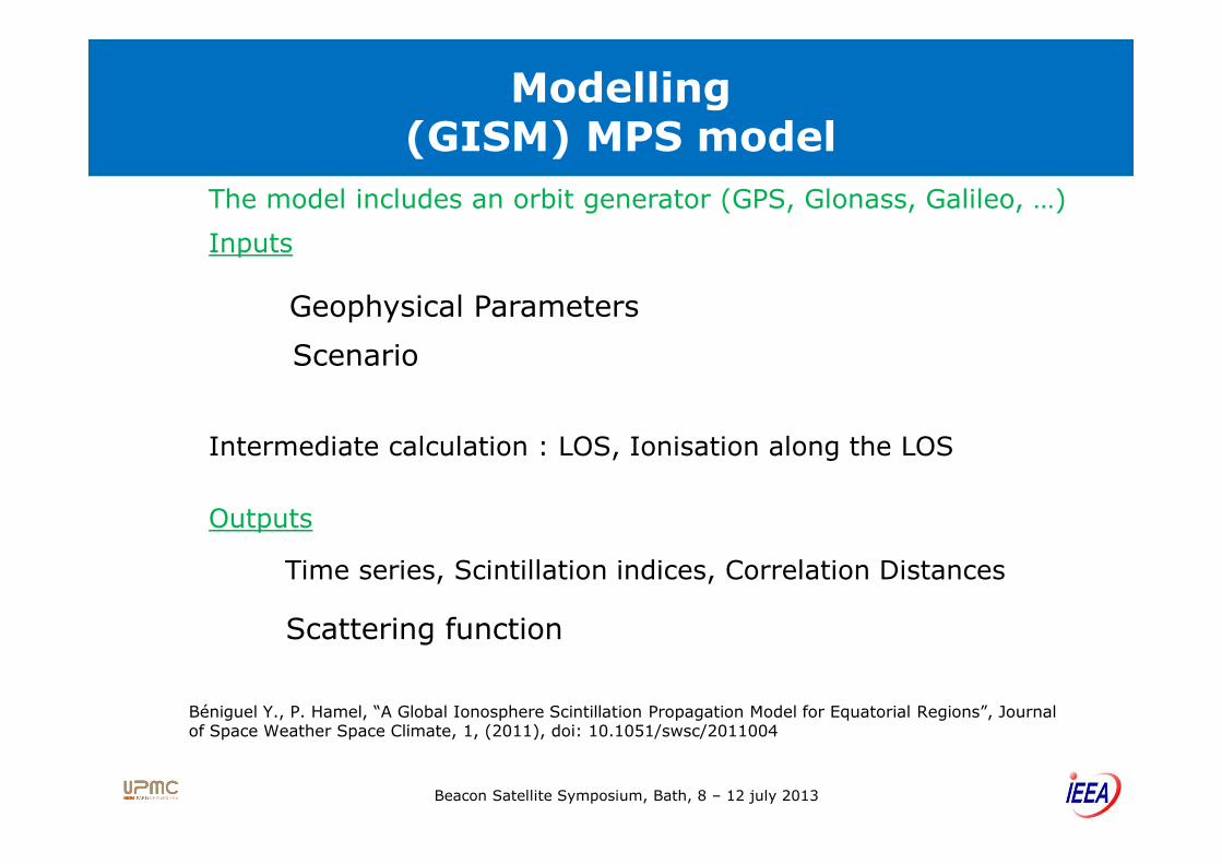
Modelling(GISM) MPS model
Inputs
Geophysical Parameters
Scenario
The model includes an orbit generator (GPS, Glonass, Galileo, …)
Intermediate calculation : LOS, Ionisation along the LOS
Beacon Satellite Symposium, Bath, 8 – 12 july 2013
Outputs
Intermediate calculation : LOS, Ionisation along the LOS
Scattering function
Time series, Scintillation indices, Correlation Distances
Béniguel Y., P. Hamel, “A Global Ionosphere Scintillation Propagation Model for Equatorial Regions”, Journal of Space Weather Space Climate, 1, (2011), doi: 10.1051/swsc/2011004

0
0.2
0.4
0.6
0.8
1
-40 -20 0 20 40 60 80 100
S4 all satellitesCayenne days 314 to 319 : year 2006
PRN2PRN13PRN10PRN4PRN24PRN28PRN17PRN12PRN8PRN29PRN26PRN9PRN6PRN23
S4
Samples with S4 < 0.2 were ignored (noise level)
Modelling vs Measurements(Intensity)
Measurements
Beacon Satellite Symposium, Bath, 8 – 12 july 2013
LT
0
0.2
0.4
0.6
0.8
1
18 19 20 21 22 23 24 25
Cayenne day 314 / 2006GISM
132327817284102429226596
S4
LT
Modelling

0
0.2
0.4
0.6
0.8
1
-40 -20 0 20 40 60 80 100
Sigma Phi all satellitesCayenne, days 314 to 319 / year 2006
PRN2PRN13PRN10PRN4PRN24PRN28PRN17PRN12PRN8PRN29PRN26PRN9PRN6PRN23
Sig
ma
Phi
(ra
dian
)
LT
The phase RMS value is slightly lower than the S4 valueSome samples exhibit high
Modelling vs Measurements(Phase)
Measurements
Beacon Satellite Symposium, Bath, 8 – 12 july 2013
0
0.2
0.4
0.6
0.8
1
18 19 20 21 22 23 24 25
Cayenne day 314 / 2006G ISM
132327817284102429226596
Sig
ma
phi
LT
Some samples exhibit high values (both measurements and modelling) due to the phase jumps
Modelling

Comparison with MeasurementsYear 2011 / Guiana / Novatel Measurements
0.6
0.8
1
S4 Calculated (GISM) in CayenneLatitude 4°8 Longitude 37°6 year 2011
0.7
0.8
0.9
1
S4 Measurement in CayenneLatitude 4°8 Longitude 37°6 year 2011
Beacon Satellite Symposium, Bath, 8 – 12 july 2013
0.2
0.4
0.6
0 50 100 150 200 250 300Doy
0.2
0.3
0.4
0.5
0.6
0 50 100 150 200 250 300
Doy

Kriging Algorithm
Beacon Satellite Symposium, Bath, 8 – 12 july 2013
Kriging Algorithm
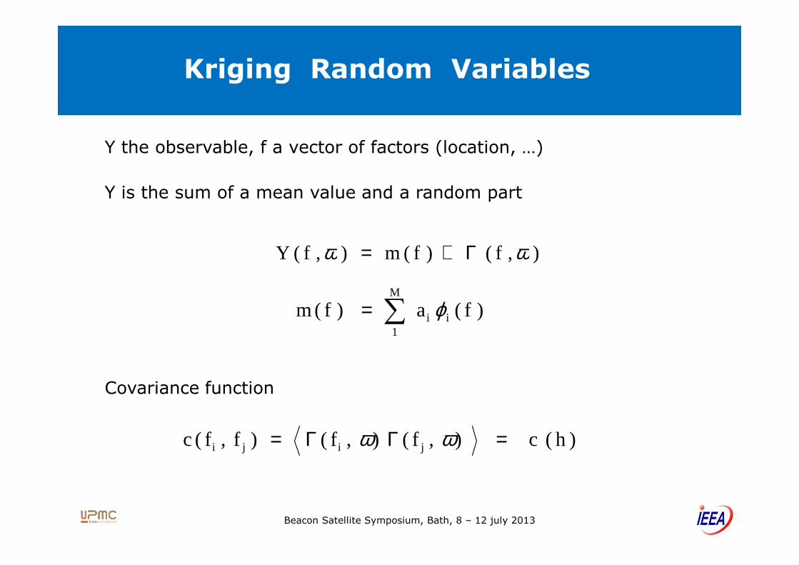
) , f ( ) f ( m ) , f ( Y ωω Γ+=
Y the observable, f a vector of factors (location, …)
Y is the sum of a mean value and a random part
Kriging Random Variables
Beacon Satellite Symposium, Bath, 8 – 12 july 2013
) f ( a ) f ( m i
M
1i ϕ∑=
)h ( c ) , f ( ) , f ( ) f , f ( c jiji =ΓΓ= ωω
Covariance function

Covariance Function
� Few data points
� Many data points
Computation of the experimental covariance
Beacon Satellite Symposium, Bath, 8 – 12 july 2013
� Few data points
Choice of the covariance function among known models.

Kriging Interpolation Technique
) , f ( Y *Y j
N
1 j ωλ∑=
A linear estimator is built with all data points
The outcome at f0 is linear
Beacon Satellite Symposium, Bath, 8 – 12 july 2013
The estimator gives an exact value at the data points
(Lagrange multipliers)
) f ( Y ) c , f , (f ) f ( *Y N
1jj0 j 0 ∑= λ
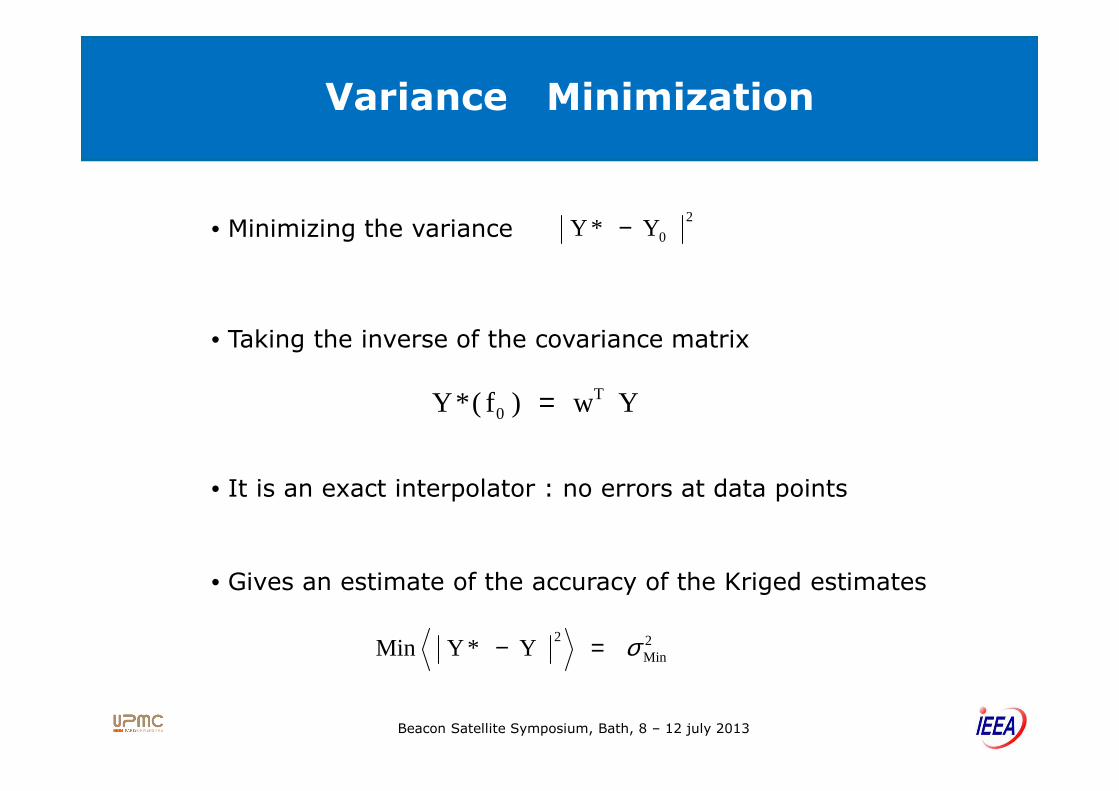
Variance Minimization
2
0 Y *Y −• Minimizing the variance
• Taking the inverse of the covariance matrix
Y w ) f ( *Y T=
Beacon Satellite Symposium, Bath, 8 – 12 july 2013
Y w ) f ( *Y T0 =
• It is an exact interpolator : no errors at data points
• Gives an estimate of the accuracy of the Kriged estimates
2Min
2 Y *Y Min σ=−
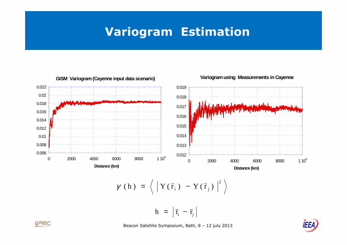
Variogram Estimation
0.014
0.016
0.018
0.02
0.022
GISM Variogram (Cayenne input data scenario)
0.016
0.017
0.018
0.019
Variogram using Measurements in Cayenne
Beacon Satellite Symposium, Bath, 8 – 12 july 2013
r r h ji −=
) r ( Y ) r ( Y )h ( 2
j i −=γ
0.006
0.008
0.01
0.012
0 2000 4000 6000 8000 1 104
Distance (km)
0.012
0.013
0.014
0.015
0 2000 4000 6000 8000 1 104
Distance (km)

Variograms Estimated on a Reduced Time Duration
Experimental variograms based on GISM calculations
Beacon Satellite Symposium, Bath, 8 – 12 july 2013
S4 variogram variogramϕσ

Covariance Function
)h ( T )h ( C γ−= 4 10 4.7 T −=with
Beacon Satellite Symposium, Bath, 8 – 12 july 2013
range
T

Reference data Kriged data
Beacon Satellite Symposium, Bath, 8 – 12 july 2013
Results of S4 data kriging
Reference data
Kriging data
Kriged data

Cut at Latitude 6°
Beacon Satellite Symposium, Bath, 8 – 12 july 2013
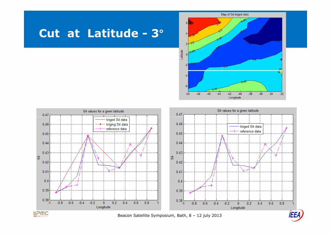
Cut at Latitude - 3°
Beacon Satellite Symposium, Bath, 8 – 12 july 2013

Cut at Latitude – 3°
Beacon Satellite Symposium, Bath, 8 – 12 july 2013

Cut at Longitude - 44°
Beacon Satellite Symposium, Bath, 8 – 12 july 2013

Cut at Longitude - 44°
Beacon Satellite Symposium, Bath, 8 – 12 july 2013

Cut at Longitude - 36°
Beacon Satellite Symposium, Bath, 8 – 12 july 2013

Coupe de SigmaPhi pour
une longitude de -36°
Cut at Longitude - 36°
Beacon Satellite Symposium, Bath, 8 – 12 july 2013

Kriging Over a Whole Year
Beacon Satellite Symposium, Bath, 8 – 12 july 2013
The covariance function used was
deduced from GISM calculationsLima 2012
Dip Lat. 0°65

Conclusion
Analysis of scintillations using the IGS network
Improve the calculation of the variogram
(Comparison to 50 Hz data)
Beacon Satellite Symposium, Bath, 8 – 12 july 2013
Improve the calculation of the variogram
(Time as an additionnal factor)
Produce the error maps

Thank you
Beacon Satellite Symposium, Bath, 8 – 12 july 2013