iowa’s arctic research dimension
DESCRIPTION
ARCTSET: Arctic, Remote and Cold Territories Social and Environmental Trends Research Group @University of Northern Iowa (UNI). Iowa’s Arctic research dimension. Arctic Wildfires and Clime Change: A Spatial Longitudinal Analysis Using MODIS Data. CORRESPONDENCE TO ENVIRONMENTAL CONDITIONS. - PowerPoint PPT PresentationTRANSCRIPT

ARCTSET:Arctic, Remote and Cold Territories
Social and Environmental TrendsResearch Group
@University of Northern Iowa (UNI)
Iowa’s Arctic research dimension

This study aims to conduct an exploratory spatiotemporal analysis to reveal spatial patterns and temporal fluctuations of wildfire events in the Arctic. Tundra wildfires have an important impact on arctic ecosystems as they can substantially alter the amount of biomass and animal abundance in affected areas. The knowledge base about tundra wildfires is limited. Most fires take place in remote areas and remain unmonitored from the ground or air. This study uses MODIS-derived active fire data to analyze spatial and temporal patterns of tundra wildfires between 2004 and 2008. The dataset incorporates locations of active fire events and estimates of fire radiated power (FRP).In 2004-2008 MODIS sensors registered over 3,000 fire events. The largest number of fire events was recorded in 2005. The wildfires exhibit clear seasonality determined by seasonal changes in tundra landscapes with most fires occurring in July and August. We observed inter-year fluctuations when a fire season either started earlier (in June) or lasted longer (in to September). The wildfires demonstrate a tendency to cluster, although year-to-year locations of clusters vary. Wildfires concentrated in Alaska and in Northwestern and Northeastern Russia. This is also true for the intensity of fires: in the five-year period the FRP values in some areas exhibited considerable spatial autocorrelation.To analyze possible factors that determine spatiotemporal variation of arctic wildfires occurrence and intensity, we analyzed fire events in respect to geographic location (latitude/longitude), climate parameters, vegetation types and proximity to points of human-caused disturbance (settlements, roads, pipelines, oil wells, etc.). The results clearly indicate the relationship between vegetation types and occurrences and intensity of wildfires: areas with larger amounts of combustible biomass and longer warm periods having a greater number and more intensive fires. We were unable to detect a clear relationship between wildfire locations and elements of anthropogenic disturbance.
Identify spatial (distribution and clustering) and temporal patterns (seasonal and multiyear) of arctic wildfire events and their intensity characteristics Analyze relationships between wildfire occurrence and intensity and environmental conditions
Wildfire data [FIRMS]:Fire events: detected fire occurrences (confidence >= 50)Fire Radiative Power (FRP): a measure of radiant heat output of detected fires in MegaWatts (MW) derived from MODIS Data Processing System (MODAPS) Collection 5.1 Active Fire Products
Other data:oClimate variables [U Delaware]oVegetation and bioclimatic variables [CAVM]oHuman-caused disturbance
Exploratory Analysis:oTime series analysis: character and fluctuations in seasonality and multiyear patternsoAnalysis of spatial distribution : evidence of spatial clustering (NN, Ripley’s K), spatial autocorrelation and fire hot-spots (Moran’s I , Geary’s C, LISA)Explanatory Analysis: (correlation analysis using wildfire environmental factors/drivers and grid and zonal aggregates of fire occurrences and intensity) oSpatial correspondence with temperature and precipitationoSpatial correspondence with vegetation types and biomassoSpatial correspondence with human-induced disturbances
Spatiotemporal characteristics of wildfires: Seasonality with most fires occurring in July and August. In some years a fire season either started earlier (in June) or lasted longer (in to September). Multiyear geographical consistency: concentrated in Alaska, NE and NW Russia. More intensive and frequent fires are concentrated in Alaska and NE Russia.Clustering and autocorrelation in intensity characteristics: tend to form localized isolated clusters, often of high intensity.
Relationships with environmental factors:Both fire occurrences and intensity are positively associated with temperatures in spring, and intensity with temperatures in May and August. More intensive fires correspond to higher temperatures in August and September.Fire intensity declines with higher precipitation in August, September and winter.Areas with more combustible biomass have a greater number and more intensive wildfires.No clear relationship between wildfire locations and anthropogenic disturbance.
Research Objectives
Summary
Arctic Wildfires and Clime Change: A Spatial Longitudinal Analysis Using MODIS Data
Total Fires By Year And Month Average FRP by Year and Month
Number of Fires by Region
Results:ARCTIC FIRES SPATIAL AND SEASONAL DISTRIBUTION
CORRESPONDENCE TO ENVIRONMENTAL CONDITIONS
Methodology
Data Clustering: Ripley’s K Function
Hot Spot Analysis LISA Analysis
SPATIAL CLUSTERING, HOT-SPOTS
Correspondence with climatic parameters
MEASURE STATISTICS OBSERVATIONSAverage Nearest Neighbor [Clark-Evans
Index]R = 0.05;
z = -105.6 st dvClustered; significant
Global Moran’s I (FRP)I = 0.13;
z = -105.2 st dv;Threshold Distance = 100 km
Positive autocorrelation significant


Creative Arctic: Understanding the Role of Creative Capital in the Circumpolar North
Andrey N. Petrov, University of Northern Iowa, USA
Creative Arctic: Understanding the Role of Creative Capital in the Circumpolar North
Andrey N. Petrov, University of Northern Iowa, USA
ABSTRACTThe vast majority of studies in economic geography of talent and creativity have focused on large metropolitan areas and core regions. However, I argue that the creative capital is an equally necessary factor (an agent of economic transformation and revitalization) in the northern frontier. This theoretical account serves as the basis for the empirical study into the economic geography of talent and creative capital in the Canadian North. The paper advances the two-ring-four-sector approach to define the creative class structure. It extends the creative capital metrics to measure four ‘sectors’ of the creative class: scientists (“talent”), leaders, entrepreneurs and bohemia. The empirical part of the paper applies the extended creative class metrics at two different scales. The findings for 288 Canadian regions suggest that the geographic distribution of the creative capital is uneven and heavily clustered in major urban centers. However, some frontier regions appear to perform exceptionally well in all rankings. The in-depth analysis of 34 communities in the Canadian North identifies creative clusters in economically, geographically and politically privileged communities that serve as creative ‘hot spots.’ Thus, contrary to the metropolitan bias, these results indicate that northern communities are not ‘hopeless places’ fully deprived of the creative capital. Creative ‘hot spots’ in the Canadian North exist, and could become the centers of regional reinvention, if appropriate policies are introduced in support.
RESEARCH OBJECTIVESRethink and revise the creative capital approach to economic development to make it applicable in the North Develop creative capital metrics appropriate for northern communitiesConduct an exploratory analysis of the creative capital in the Canadian North
METHODOLOGYDevelop and test creative capital metrics
RESULTSTest dependencies between CC, attractiveness and specialization
CONCLUSIONSCreative capital (CC) is pivotal for the economic path-creation in northern regionsMost CC-economic development relationships found in the metropolis are maintained in the NorthThe nature and composition of the creative capital in the North is different, so are its interactions with other forms of capital, particularly social and civic. Direct application of Florida’s scripts to peripheral communities does not appear appropriateThe four-sector approach provides a more complete and sophisticated understanding of the creative capital, It is more accurate for the peripheryOther attractiveness factors must be considered: relation with Aboriginality, role of women in the communityCC structure: evidence of both intergroup clustering and disproportions. The North most seriously lacks the entrepreneurship and leadership components of the CCIn the North there were localized concentrations of the creative class, included Yellowknife, Whitehorse, Iqaluit, Inuvik, Fort Smith, Smithers
Creative class metrics (Characteristics of the creative class) Construct to be measured Traditional measures
Talent Index (TI) is a location quotient of the population over 20 years of age who have a university degree.
Level of formal education of the labour force
Bohemian Index (BI) is a location quotient of the employment in artistic and creative occupations: “Art and Culture” (NOC group F)
Creative class: bohemians
Additional (new) measures Leadership index (LI) is a location quotient of people with leadership and managerial occupations (NOC group A);
Creative class: leaders
Entrepreneurship index (EI) is a location quotient of people with business occupations (NOC group B);
Creative class: entrepreneurs
Applied science index (ASI) is a LQ of people with applied science occupations (NOC group C);
Creative class: scientists
Quality of Human Resources Index (QHRI) is an integral indicator that combines the educational and professional characteristics of population and is defined and a half-sum of the proportions of people with university degree and a creative occupation
A degree to which the region’s labour force has university education and engaged in
creative professional activity Creative Drive Index (CDI) is calculated by multiplying the TI by LI (i.e. by combining talent and leadership).
“Power” of the creative drive in a region
Measures of ‘quality of place’ (characteristics of attractiveness to the creative class)
Traditional measures Mosaic Index (MI) is a location quotient of the total population that is foreign-born. Society’s diversity Visible Minority Ratio (VMR) is a location quotient of visible minorities in total population.
Society’s diversity
Additional (new) measures Common Law Couples Ratio (CLCR) is a location quotient of population in common law relationship.
Society’s tolerance
Feminist Index (FI) is a location quotient of women in managerial (leadership) occupations
Society’s openness, “low barriers of entry”
Aboriginality Index (AI) is a location quotient of people with Aboriginal identity (by the Census definition) in total population.
Presence of Aboriginal population
Resource-dependency Index (RDI) is a location quotient of employment in the occupations unique for the primary sector.
A degree of resource-reliance
Measure of technology sector specialization Tech-Pole Index (TPI) is a location quotient of the employment in North American Industry Classification System (NAICS) high technology sectors (information and cultural industries and professional, scientific and technical services).
Specialization in technology sectors
Components
1 2BI .924LI .858 .269
CDI .802 .535QHRI .779 .598
EI .664 .536TPI .578 .592TI .570 .692
ASI .959
Percent of variance
49.3 34.4
IndicesCDI QHRI TPI TI BI LI EI ASI MI VMR CLCR FI AI RDI
CDI 1.000.950*
*.712*
*
.872**
.835**
.876** .744**.559*
*.370* .411* .227 .692** .523** -.504**
QHRI 1.000.735*
*.890*
*.819*
*.817** .849**
.613**
.302 .328 .293 .622** .568* -.575
TPI 1.000.692*
*.596*
*.597** .679**
.545**
.531**
.379* .069 .429* .145 - .398*
TI 1.000.701*
*.563** .633**
.636**
.356* .369* .180 .360* .256 -.521*
BI 1.000 .743** .644** .297 .202 .209 .338 .597** .527** -.472*LI 1.000 .723** .354* .292 .276 .178 .886** .697** -.432*
EI 1.000.537*
*.204 .340* .315 .485** .551** -.587**
ASI 1.000 .294 .486* .214 .126 .195 -.305
MI 1.000.694*
*-.540** .305 .035 -.132
VMR 1.000 -.189 .192 .157 -.150
CLCR 1.000 .042 .276 -.179
FI 1.000 .667** -.213
AI 1.000 -.227
RDI 1.000
Rank Rankling 1: creative class Rankling 2: creative class ‘pull-factors’
1 2 3 4 5 6 7 8 9 10 11 12 13 14 15 16 17 18 19 20 21 22 23 24 25 26 27 28 29 30 31 32 33 34
Yellowknife Whitehorse
Iqaluit Fort Smith Smithers Inuvik
Rouyn-Noranda Rankin Inlet Thunder Bay Slave Lake
Chicoutimi-Jonquiere Hay River Val-d’Or
Prince George Baie-Comeau
Sault Ste Marie Fort McMurray Kirkland Lake
Alma Thompson
Happy Valley-Goose Bay Elliot Lake
Kenora Fort St.John
Timmins Kapuskasing Labrador City Chibougamau
Mackenzie Roberval Flin Flon
Iroquois Falls Port Cartier Greenstone
Whitehorse Yellowknife
Inuvik Elliot Lake
Iqaluit Smithers
Rankin Inlet Thunder Bay Fort Smith
Prince George Fort McMurray
Hay River Sault Ste Marie
Kenora Slave Lake
Kirkland Lake Thompson
Fort St.John Mackenzie
Rouyn-Noranda Kapuskasing Labrador City
Timmins Baie-Comeau Greenstone
Chicoutimi-Jonquiere Val-d’Or Flin Flon Happy Va
Alma Iroquois Falls
Roberval Chibougamau Port Cartier
RESULTS
DIVERSITY
TOLERANCE
OPENNESS
ABORIGINA-LITY
)
,+ creative ‘hot spots’
Aboriginal creative townslarge industrial centerssmaller industrial centers (2 clusters)(
Types of communities
)
,+ creative ‘hot spots’
Aboriginal creative townslarge industrial centerssmaller industrial centers (2 clusters)(
Types of communities
attractiveness attractiveness
Creative capital
Creative capital ranking of northern communities
‘Talent’ in the North
MOREhttp://www.uni.edu/apetrov/creativearctic.html
metrIcs
metrIcs

Coping with ‘ethanol boom’:understanding
agricultural systems’ response in America’s Heartland
Andrey N. Petrov,Matthew Voss & Ramanatan Sugumaran
University of Northern Iowa
This research is NOT funded by NSF Iowa EPSCoR

Iowa NSF EPSCoR
• Harnessing Energy Flows in the Biosphere to Build Sustainable Energy Systems – IA is 1st in ethanol production (26%)– IA is 4th in wind energy generation
• Alternative energy systems• Energy resources • Energy generation and transportation• Pending at NSF

Background
• Much is written on energy, ecological, economic, industrial, climate impacts of increased ethanol production
• Little known on coping strategies/responses in agriculture-based socio-ecological systems in the USA
• Need for a detailed spatially-explicit analysis of ethanol boom implications and responses in America’s heartland.
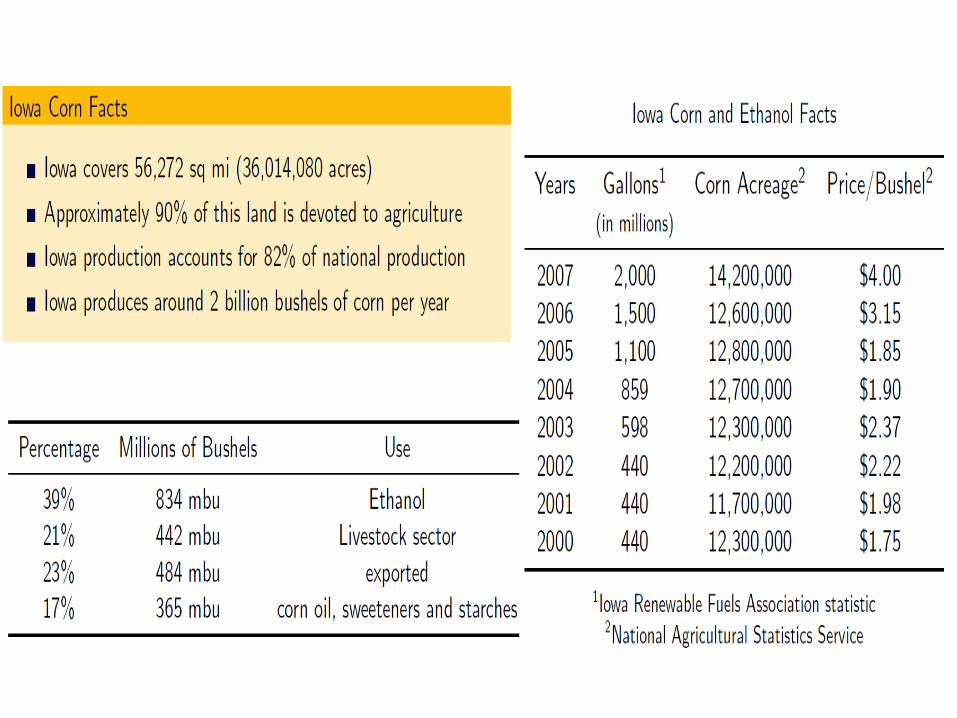
• Iowa is the main producer of corn-based ethanol


Research Tasks
• Analyze the relationship between ethanol production and land cover change [2006-07]
• Analyze the effects of ethanol on the Conservation Reserve Program lands and other vulnerable ecosystems
• Analyze the effect of ethanol on long term sustainability of agriculture:– Utilization and preservation of land resources– Maintaining crop diversity– Possible impacts on soil fertility and fertilizer use

Working hypotheses• (1) Corn production could have displaced other crops,
possibly causing a decline in crop diversity and redistribution of croplands to areas less suitable for growing crops
• (2) Increases in corn production and acreage have been largely achieved by altering crop rotation patterns with more severe rotation deviations prevalent on most fertile and productive lands.
• (3) Crop production expanded to Conservation Reserve Program lands and other vulnerable and underrepresented ecosystems (such as wetlands and wooded areas).
• (4) Proximity of ethanol plants per se does not cause corn acreage growth in particular areas.

Data
• NASS crop acreage and harvest statistics (2000-08)
• NASS Cropland Data Layer (2000-08)• SSURGO (Soil Survey) soil data; CSR – corn
Suitability Rating• FSA Crop Reserve Program data (CRP lands)

Data pre-processing & Issues
• CDL is based on different imagery - need to resample to make comparable
• Most comparable CDLs: 2005, 2006 and 2007 (same imagery source)
• CDL accuracy 95% for most large crops, but only 50% for some smaller crops
• Buffer ethanol plants (15 and 30 miles); separate models run for 2003, 2004 and 2007
Measuring crop rotation
• Corn-soybeans and corn-corn-soybeans are accepted rotation patterns
• Deviation: corn-corn-corn… (corn at least for three consecutive years)
• 2000-2002 to 2005-2007

Land quality data
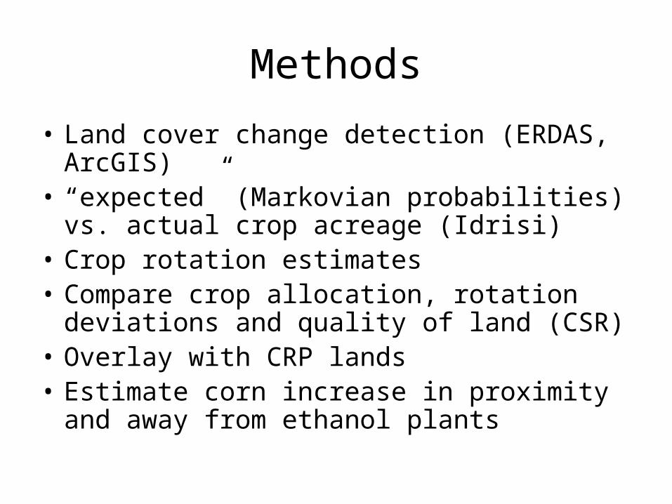
Methods
• Land cover change detection (ERDAS, ArcGIS)• “expected” (Markovian probabilities) vs. actual
crop acreage (Idrisi)• Crop rotation estimates• Compare crop allocation, rotation deviations and
quality of land (CSR)• Overlay with CRP lands• Estimate corn increase in proximity and away
from ethanol plants

Results

Increase in corn acreage
-land under corn grew 12.6%,-deviated from “expected” 17% -under soybeans dropped 15%-switch in trend comparedto the 1990s.


Displacement of ‘other’ crops and land cover types; decrease in crop diversity
2005 2006 2007 2008 Oats 210 110 67 75 Hay,
including alfalfa 1600 1500 1480 1550
Alfalfa 1250 1180 1140 1150
Land cover types replaced by corn the following season

Deviation from normal rotation cycles

Corn x 3 seasons in a row
2003-05 2004-06
2005-07
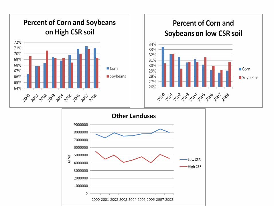
Most rotation deviations are on most fertile soils

Corn and land quality
% corn planted on low CSR decreased from 34% to 29%. cornfields area on high CSR soil increased from 66% to 71% These data give no evidence that corn was pushed to lower quality or marginal lands.An increasing area of more productive lands was allocated for growing corn. This trend reflects the tendency to address the demand to increase corn planted areas by planting the most valuable crop (corn) on most suitable soils overuse of most fertile land2007 season – highest ever use of fertilizers

CRP lands and the boom• CRP declined in 2005-2006; 2007-2009
2007 2008• Acres eligible: 500,000 330,000• Acres withdrawn in Iowa (%) 28 33• Acres withdrawn in USA(%) 15 19
• Termination of CRP contracts at the peak of the ‘boom’ in 2007 and subsequent 2008 was one of the reasons of the 13.5% CRP acreage decline in 2007-2009

Year Near plants Not Near plants

Concluding remarks: Implications of ethanol boom
• Overuse of primary lands, highest-quality soils• Rotation deviation and increased use of fertilizers• Displacement of secondary crops to less productive
soils• Decrease in crop diversity• Withdrawal from CRP, but limited (30%)• Little relationship between location of ethanol
plants and corn acreage expansion• Most coping practices are unsustainable

?