ipa05-g-006 _p011_023

8/3/2019 IPA05-G-006 _p011_023

http://slidepdf.com/reader/full/ipa05-g-006-p011023 1/13

11

IPA05-G-006

PROCEEDINGS, INDONESIAN PETROLEUM ASSOCIATION

Thirtieth Annual Convention & Exhibition, August 2005

4D SEISMIC AND ROCK PHYSICS MODELING RESPONSES TO RESERVOIR STEAM FLOOD

Muhammad Edisar*Lilik Hendrajaya*

Gunawan Handayani*

Umar Fauzi*

Laode Ngkoimani*

Yarmanto**

ABSTRACT

Time Lapse (4D) seismic and Rock Physics model

was constructed in Melati oil field on central SumatraBasin to monitoring and tracking steam flood and

production related changes in the reservoir. A model

of the reservoir steam flood was constructed for a

pattern steam flood in Area X of the field. The model

was based on a geostatistical geological model and

populated with temperature and porosity. Pressure

and saturation properties were added to provide the

necessary input for seismic modeling. Through a rock

physics model based on the core analysis of the field,

the elastic properties (Vp, Vs and density) were

determined from the reservoir properties. These

elastic properties were used to determine the seismicresponse of the model with and without steam. The

results indicated that from the rock physics modeling

using Gassmann equation, steam injection decreases

the V p by an average of 20-25% in the reservoir

sands. Rock physics analysis also show that shear

velocities are also sensitive to steam injection, with an

average decrease of 12%. However, the Gassmann

calculation results show that Vs is insensitive to steam

injection. This discrepancy is probably caused by

Gassmann's assumptions that no chemico-physical

interactions exist between the rocks and pore fluids.

Time shifts in seismic modeling events provided an

indication of the presence of steam in the overlyingreservoir. The relationship between time shift and

steam thickness was strong for thick steam, but

it was not possible to distinguish thin steam

zones from thick hot oil zones solely on the

basis of time shift. At the same time, tuning between

* Institute Technology Bandung

** P. T. Caltex Pacific Indonesia

the steams related and geologically related seismic

events influenced seismic amplitudes. It appears that

a combination of attributes is necessary to resolve the

effects of steam on the 4D seismic data acquired over the field.

INTRODUCTION

During the last two decades, a number of successful

strategies have emerged for detecting hydrocarbons

from seismic data. Most of these are based on rock

elastic properties, travel time (or velocity),

impedance, bright spots and can be understood

deterministically in terms of the compressibility and

density of the pore fluids, coupled with the stiffness

of the rock matrix. The mechanics of these elasticfluid signatures at low seismic frequencies are

described by the well-known Gassmann (1951)

relations. AVO analysis, which uses inference of both

P and S-wave impedances helps to separate pore fluid

from lithologic effects (Ostrander, 1984; Smith and

Gidlow, 1987). However, many problems remain,

especially the detection of low gas saturation, oil

water contact (OWC ), gas oil contact (GOC ) and

seismic attenuation still difficult to resolve from

seismic, using rock physic and seismic modeling and

correlated to seismic and well log data will provides

an additional discriminator for hydrocarbon indicator

(Edisar et al., 2004).

Hydrocarbon production directly affects the reservoir

properties (saturation gas, oil and water, pressure

and temperature). In order for time-lapse (4D)

monitoring to be effective, the changes in reservoir properties must cause a detectable change in the

seismic parameters (Edisar, 2000). In this case rock

physics relationships provide the bridge between the

http://gobackdoc/

http://gobackdoc/

http://gobackdoc/

http://gobackdoc/

8/3/2019 IPA05-G-006 _p011_023


12

primary reservoir properties and the seismic

parameters. 4D seismic technology is a volume

resolution enhancing used to monitoring of reservoir

parameters properties changes respect to lapse time.

Petrophysic data and seismic are important

information for static and dynamic reservoir

characterization such as porosity, saturation and fluiddistribution properties (Edisar, 2002). One of the most

common rock physics modeling processes is based onthe theories of Biot and Gassmann for determining

the properties of fluid saturated rock from the

properties of dry or air filled rock. Particular care is

taken to use realistic solid mineral properties in the

Biot-Gassman transform. For example calibrate theclay bulk modulus and density and then compute the

correct average solid moduli and density at each

depth sample. This gives more accurate results than

the common block or zone averaging approach. Fluid

properties are also carefully computed using either homogenous or “patchy” fluid mixing rules to give

the correct results. This avoids the problem of over or

under predicting fluid saturation effects that can occur

with more simplistic approaches (Edisar et al., 2004).

In this study, we attempted to understand the seismic

and rock physic of reservoir response with respect to

steam flood from a forward modeling approach. In

this methodology, a model is constructed and the

resultant seismic cube interpreted in a similar manner

to the real seismic data on the field. Since the

properties of the model are known, we can obtaininsights into the usefulness and pitfalls of different

interpretation methodologies. Comparing properties

predicted from the synthetic seismic data to the

properties used to construct the synthetic seismic data

could do this. The process of synthetic seismic

modeling involves the following steps: (1) Rock

physics modeling (2) Construction of static (facies

and porosity) and dynamic reservoir (temperature,

pressure and saturation) property earth model. (3)

Calculation of the elastic properties (Vp, Vs and

density) from the dynamic and static reservoir

properties using an appropriate rock physic model. (4)Calculation of reflectivity and convolution with an

appropriate seismic wavelet to output a synthetic

seismic model.

Interpretation of the model involved rock physics

analysis result, analysis of the amplitudes, time shifts

and reservoir properties versus the seismic parameter

caused by the presence of the steam. Despite of the

limitations, the model provides some idea of the

usefulness and potential pitfalls of relying on each of

the interpretation techniques.

ROCK PHYSICS MODELING

Fluid properties can be estimated using relationships

(Batzle and Wang, 1992). These relationships are based on empirical measurements. Fluid calculating

requires oil API gravity, gas gravity, GOR, reservoir

pressure, and temperature. Brine salinity is also

required. In case of Melati field the pore

fluid/reservoir pressure varied from 50 psi to 350 psi.

The API gravity is around 20om and salinity assumed

5000 ppm for the water. The elastic properties

(modulus and velocity) of the reservoir oil and water

were then calculated. At 350o F, water will become

steam when pressure is below 135 psi. As a result, for

simply assumed a bulk modulus of 0.2 GPa and a

bulk density of 0.2 g/cm3 for steam. Velocities inoil/water-saturated rocks were calculated using the

Gassmann equation (Gassmann, 1951):

2

2

1

)/1(

m

dry

m f

mdry

drysat

K

K

K K

K K K K

−−

+

−+=

φ φ , (1)

Where K sat is the bulk modulus of a rock saturated

with a fluid of bulk modulus K f , K d is the frame (dry)

bulk modulus, and K m is the matrix (grain) bulk

modulus of the same rock, and φ is the porosity. Theshear modulus Gsat of the rock is not affected by fluid

saturation, so that

drysat GG = , (2)

Where Gdry is the frame (dry) shear modulus of the

rock. The density ρ sat of the saturated rock is simply

given by

f drysat φρ ρ ρ += . (3)

Where ρ sat and ρ dry are the fluid-saturated and dry

densities of the rock, respectively. ρ f is the pore

fluid’s density. The frame bulk and shear moduli were

calculated using the measured velocities in the frame

rock:

⎟ ⎠

⎞⎜⎝

⎛ −= 22

3

4s pdrydry V V K ρ , (4)

8/3/2019 IPA05-G-006 _p011_023


13

2

sdrydry V G ρ = . (5)

The bulk modulus K f of the oil/water mixture was

calculated using Wood’s equation (Wood, 1930)

o

o

w

o

f K

S

K

S-1

K

1+= , (6)

Where K w and K o are the bulk moduli of water and

oil, respectively, and So is the oil saturation in

fraction. The bulk density ρ f of the oil/water mixture

is calculated by

( ) oowo f SS ρ ρ ρ +−= 1 (7)

Where

ρ w and ρ o are the bulk densities of water andoil, respectively.

In the Gassmann calculation, assumed that the pore

spaces were occupied by only water and oil no gas is

present and also assumed a grain (matrix) bulk

modulus , K m, of 38 GPa for the sands and shales and

76 GPa for other samples with high grain densities.

For each sample selected for temperature

measurements from 75o to 350o F, on the velocities,

which is defined as (Wang, 2001)

( ) %10075

75350% xF Vat

F Vat F Vat V o

oo

−=∆ (8)

Where V can be either compressional (V p) or shear

(V s) velocity.

At 350o F, water in the pore space will transform to

steam whenever the reservoir pore fluid pressure

drops below 135 psi. Therefore, the measured

velocity changes at 100 and 50 psi are caused by both

the temperature increase and the presence of steam.

Since define the effect of steam injection at these

reservoir pressures on the measured and calculatedseismic properties as, here V p as an example

(Wang, 2001).

%100

75

75350 ×−

=∆F p

F pF p

po

oo

V

V V V , (9)

Where V p350o F and V p75o F are the measured

compressional velocities at 350o F and 75o F,

respectively.

The changes in seismic properties in the above

discussion are caused by the combined effect of

increase in temperature and presence of steam in the

rock. For each sample, also tried to separate the effect

of temperature from that of steam. Assuming that

there was no free steam in the pore space so that the

effect of temperature alone can be defined as (V p asan example)

%100

75

75350 x

MeasV

MeasV ExtrpV V

F p

F pF p

p

o

oo −=∆ (10)

The effect of steam alone is therefore defined as

%100

350

350350 x

ExtrpV

ExtrpV MeasV V

F p

F pF p

p

o

oo −=∆ (11)

The effect of steam alone was calculated using the

extrapolated seismic properties, assuming no phase

changes in the pore fluids, at 100-psi reservoir pore

pressure and 350o F. By comparing the extrapolated

data with the measured data, one is able to quantify

the effect of steam in the pore space on the seismic

properties. The changes in seismic properties due to

the presence of steam can be correlated to porosity.

For the velocity changes (Wang, 2001),

118.2153.0 −−≈∆ φ p

V (12)

5.011.0 +≈∆ φ s

V (13)

Where ∆V p and ∆V s are the percentage changes in

compressional and shear velocities,φ=Porosity

P and S wave velocities increase with pressure.

Increasing pressure closes cracks and pores in the

rock frame. Two types of pressure affect seismic

velocities; Overburden pressure: Combined weight of

rock and fluids above reservoir (Mavko et al, 1998).

( )dz zgS z

b∑=0

ρ (14)

Normal gradient is 1.0 psi/ft or 0.0225 MPa/m

Hydrostatic ( pore or reservoir ) pressure weight of the

fluid column

gzP fl H ρ = (15)

8/3/2019 IPA05-G-006 _p011_023


14

Normal gradient is 0.465 psi/ft or 0.0105 MPa/m.

Where g is gravity, ρ b and ρfl are bulk and fluid

density respectively and z is depth. Seismic velocity

is primarily influenced by effective pressure:

H eff PSP −= (16)

The rock physics and seismic modeling relationships

are based on real core data measured on frame rocks

that allows one to model seismic responses to fluid

saturation and pressure changes. The frame bulk and

shear moduli were calculated using the measured

velocities and bulk densities. Statistical relationships

between the frame bulk and shear moduli and

porosity were obtained through linear correlations

(Wang, 2001)

φ baK dry += (17)

And

φ d cGdry += (18)

Where porosity φ is in fraction, K dry and Gdry are in

GPa (Gigapascal).

In order to obtain meaningful statistical relationships,

normally measured a large number of samples from

each reservoir/field to minimize the effect of

heterogeneity and scaling. The coefficients a, b, c,and d in equations (17) and (18) are obviously

dependent on the net overburden pressure. It is the net

overburden pressure (also called differential pressure

or sometimes effective pressure) that governs the

elastic properties of reservoir rocks. Therefore further

we can correlate the coefficients a, b, c, and d to the

net overburden (effective) pressure Peff

eff eff o PaPaaa 21 ++= (19)

eff eff o PbPbbb 21 ++= (20)

eff eff o PcPccc 21 ++= (21)

eff eff o Pd Pd d d 21 ++= (22)

Where the net overburden (effective) pressure. Peff is

in psi. For the correlations on all the measured Melati

sands. The correlation coefficients result are listed in

the (Table.1).

BUILDING THE MODEL

The input object for the seismic modeling tools arethe Sgrid in depth, porosity, water saturation, oil

saturation, gas saturation, P-wave velocity, density,

facies, pore pressure, temperature, solvent saturation

and S-wave velocity. In this case we looked at for

Duri Technical Team, PT. CPI, built a style of simulation model. The porosity, permeability and

temperature were geostatistically simulated across the

Area-X 7-spot steam pattern of Melati field central

Sumatra basin (Figure 1a). Vertical cell thickness

averaged 0.8 feet (0.25m). It was necessary to add pressure and saturation properties, and to modify the

temperature property. Simulation model for steam

rigorous fluid modeling average porosity by layer no

lateral heterogeneity spatially symmetrical, pressure

was determined from consideration of the likely

bottomhole pressure in the injectors and producers

(Figure 1b). Geological model for steam, temperature

simulated from logs greater variability in steam

thickness multiple steam zones closer to complex

reality (Figure 1c). Stratigraphic framework to

synthetic seismic modeling (Figure 1d). Temperature

was reset to a constant gradient where the temperaturewas less than 350F (176C). It was necessary to ensure

that temperature and pressure conditions were

appropriate for steam generation. Saturations was

assigned on the following basis:

Initial Conditions

Water: Sw0 = 1.45 log {Permeability}-0.37

Oil: So0 = 1-Sw

Gas: Sg0 = 0.0

Steam: Ss0 = 0.0

Temp: Tm0 = 90+0.262.Depth (TVDSS)

Steamed Conditions

Sw1 = Sw0 x 0.9 for Temp change > 210F

So1 = So0 x 0.117 for Temp Change > 210F

Sg1 = 0.0

Ss1 = 1-Sw-So-Sg

Temp: Reset to 90+0.262.Depth (TVDSS)

Where Tm < 176C

8/3/2019 IPA05-G-006 _p011_023


15

Because temperature was built using the temperature

of observation (TO) wells, and not including the

injection wells, the greatest steam thickness is located

over the TO wells, and not the injectors. The

temperature logs also show a broad decline above and

below hot zones, and it was necessary to remove this

for the model to adequately generate a seismicresponse to steam. Review of the model after analysis

showed that there was more steam in the model thanwas likely in the real subsurface. The wireline logs

show that the amount of steam in the section occurs in

much more limited intervals than the temperature

profile. The temperature logs taken on their own

therefore appear to over-estimate the amount of steamin the subsurface. Despite this, the decision was taken

to use this model since it provided an appropriate

variety of geological and steam conditions.

CALCULATION OF ELASTIC PROPERTIES

The function of this step is to transform the reservoir

properties ( porosity, facies, saturation etc) into elastic

properties (Vp, Vs, Density). Using the Batzle-Wang

relationships (Batzle and Wang,1992), the elastic

properties Vp, Vs and Density were determined for the

sands of the reservoir using a rock physics model

built from the core analysis carried on Melati field

samples (Edisar et al., 2004). The fluid properties

necessary for these equations were: Gas-oil Ratio: 0,

Oil Gravity: 20 degrees API, Water Salinity: 5000 ppm. The dry frame bulk (K ) and shear (G) moduli

were determined from the following relationships

(Wang, 2001)

+++= eff eff odry PaPaaK 21

)eff eff o PbPbb 21 ++φ (23)

+++= eff eff odry PcPccK 21

( )eff eff o

Pd Pd d 21

++φ (24)

( ) ( )φ ρ ρ −= 1/ 3

graindry cmg (25)

Where the scalar in this equation are derived from

core analysis (Table 2).

Peff =( Lithostatic Pressure – Pore Pressure) in psi,

ρ grain = 2.64 g/cm3and φ = Porosity.

While the dry frame and fluid properties were

combined to generate the fluid-saturated bulk and

shear moduli, and density, using the Gassmann

equation in equation (1), (4), (5) and (7 ) the above.

SEISMIC MODELING

The seismic modeling step inputs the Vp, Vs and

Density properties, converts from time to depth,

determines reflectivity with offset and outputs the

convolved seismic trace. At each XY location, PP and

PS reflection mode are derived from Aki-Richards

(1980)

( ) ( ) s

s

s p

p

S pp V

V

V pV

V

V p R

∆

−

∆

⎟ ⎠

⎞

⎜⎝

⎛

+

∆

−=

22222

4cos2

1

41 θ ρ

ρ (26)

( )−

∆

⎪⎩

⎪⎨⎧

⎟⎟ ⎠

⎞⎜⎜⎝

⎛ −⎟⎟

⎠

⎞⎜⎜⎝

⎛ =

s

s

s p

ss

p

psV

V

V V

V pV

pV R

ϕ θ

ϕ

coscos44

cos2

222

( ) ⎪⎭

⎪⎬⎫∆

⎟⎟ ⎠

⎞⎜⎜⎝

⎛ +−

ρ

ρ ϕ θ

s p

ss

V V

V pV coscos221 222

(27)

( ) ( ) ρ ρ

θ θ ∆

−+∆

⎟ ⎠

⎞⎜⎝

⎛ −=

22222

12

14cos2

1

2

1 pV V

V V p R s

s

sSss (28)

Where:

θ sin

pV p = ; θ ϕ 2sin1cos ⎟

⎟ ⎠

⎞⎜⎜⎝

⎛ −=

p

s

V

V

Seismic reflection models deal with the interface

between the top (or base) and what is above it (or

below it). To determine the acoustic impedancechange at the interface for normal incidence set θ = 0,then the equation can be written as:

( ) ( ) ) ( ) ( ) )

( ) ( )( ) ( ) ( )( )nn pnn p

nn pnn p

PV V

V V I

ρ ρ

ρ ρ

+

−=

++

++

11

11(29)

Where n = 1, 2, 3,… N (number of layer )

8/3/2019 IPA05-G-006 _p011_023


16

To build of seismic modeling, specify the source-

receiver offset ranges that we wish model. These

offsets will be converted to incident angles for the

reflectivity calculation. Noffset is the number of

offsets, Offset0 is the first offset, and ∆offset is the

increment. Note that:

( ) Offset Noffset MaxOffset ∆−= 1 (30)

Reflectivity was determined for the 8 offsets in the

range 0-975 feet (0-297m). Each offset was

convolved with zero phase Butterworth filter of 10-70

Hz frequency with 36dB/octave roll off at either end.

The offset traces were stacked to produce a single

trace at each location.

ROCK PHYSIC MODEL ANALYSIS

Calculated P-wave and S-wave impedances are using

the bulk density and compressional and shear

velocities. The velocities and bulk density were

calculated using the Gassmann equation and the

measured dry frame rock properties under reservoir

saturation, pressure, and temperature conditions. All

the samples were saturated with oil at Ssteamirr . For

laboratory steam flood experiments, the samples were

re-saturated with reservoir-equivalent hydrocarbon oil

at irreducible steam saturations. Steam flood was

performed and seismic properties were monitored.

The measured magnitude of V p changes as the oil

saturated (at irreducible steam saturation) samplesare flooded with steam at a constant net overburden

pressure (Table 1). The results indicated that from the

rock physics modeling using Gassmann equation,

steam injection decreases the V p by an average of 20-

25% in the reservoir sands (Figure 2). The analysis

also shows that shear velocities are also sensitive to

steam injection, with an average decrease of 12%.

However, the Gassmann calculation results show that

Vs is insensitive to steam injection. This discrepancy

is probably caused by Gassmann's assumptions that

no chemico-physical interactions exist between the

rocks and pore fluids. Velocity changes as a functionof pressure and temperature (Figure 3), velocity

decreases during the primary production cycle before

steam injection due to the presence of evolved

hydrocarbon gas (point 1 to 2). At the beginning of

steam injection the free gas is pushed back into

solution and there is a velocity increase (point 2 to 3).

As steam injection continues, a velocity decrease is

due to heat (point 3 to 4) and finally due to steam

(point 4 to 5). From the rock physics modeling and

analysis resulted sand properties parameters

(Table 2). These parameters will be used for synthetic

seismic modeling.

INTERPRETATION OF THE SYNTHETIC

SEISMIC MODEL

The seismic response to steam flooding is manifestedin two key attributes amplitude and time shift. There

are other potential attributes Vp/Vs ratio from the

amplitude gradient of the prestack gathers, and

measures of attenuation through the low impedance

steam zones, but these were not investigated in thismodeling workflow, but represent possible avenues to

explore in the future. The time section summarizes

the results of the synthetic seismic model of pre-

steam and steamed (Figure 4). There are a number of

events on the pre-steam model that are generated bythe static geological model. The steamed model

shows two additional seismic reflections from the top

and base of the steam zone. At the top of the steam

there is an increase in amplitude where the top steam

event constructively interferes with the Top Pertama

seismic event. At the base of steam there is

destructive interference between the base steam and

Top Kedua seismic event. The implication is that

amplitude is potentially affected by interference

between the steam and the geological seismic

markers. While this potentially complicates the

interpretation of the seismic amplitudes, it also potentially provides information as to the location of

the steam within the section, and the proximity of the

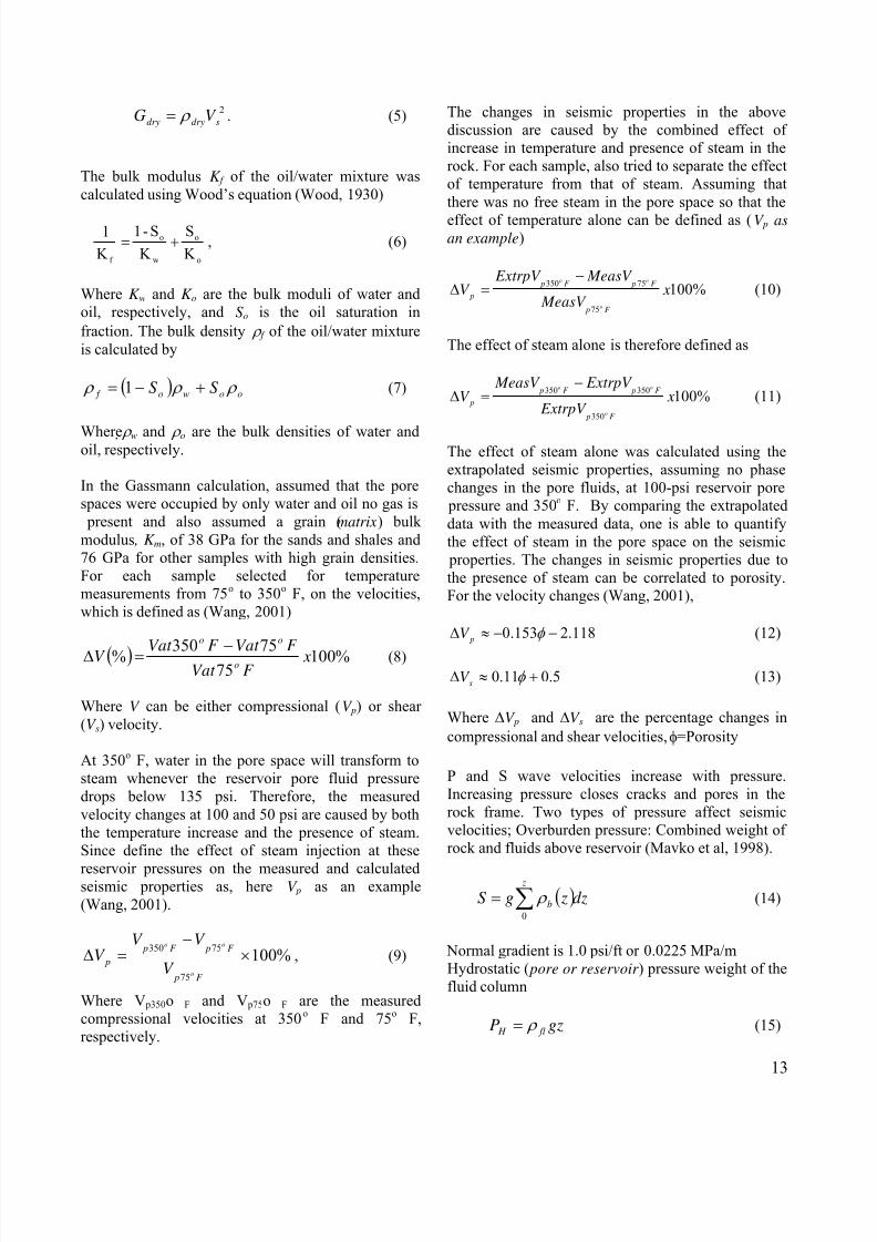
steam to the Top Pertama and Kedua. To compare the

synthetic seismic modeling section correlated to the

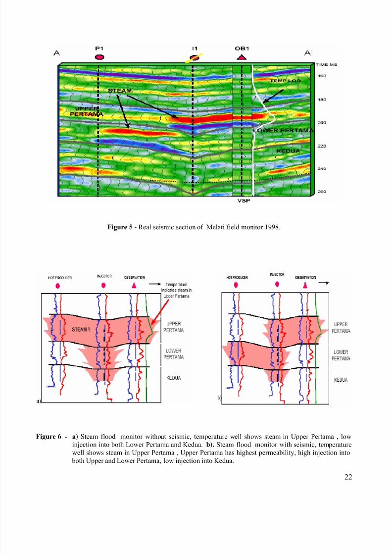
monitor real seismic section (Figure 5). If we view

steam flood monitoring from well log data only, on

the (Figure 6) we can see that steam distributions are

different using seismic and without seismic. Without

seismic (Figure 6a) shows temperature well steam in

Upper Pertama has high injection and both low

injection into Lower Pertama and Kedua. Steam flood

monitoring with seismic (Figure 6b), the temperaturewell shows steam in Upper Pertama has highest

permeability, also the data indicates high injection

into both Upper and Lower Pertama, low injection

into Kedua.

The time shift is caused by the change in interval

transit time of the reservoir, and results from the

decrease in P-wave velocity due to steam. The

expected response can be calculated from the input

8/3/2019 IPA05-G-006 _p011_023


8/3/2019 IPA05-G-006 _p011_023


18

2) Time shifts should play a role in the interpretation

of the steam flood response, but the attribute is

poor at distinguishing thick hot oil zones from

thin steam zones. It is at best an indicator of heat.

3) Horizon-based methods for determining time shift

should work for strong events below the steamedzone, where there is not interference between

steam and geological seismic events.

4) Cross-correlation methods will work better for

horizons closer to the steam zone, where there is a

possibility of interference between steam and

geological seismic events.

5) Amplitudes may be a useful indicator of steam,

except where the steam is thick enough to cause

interference with high amplitude geologically

related seismic events. Recognition of where thisoccurring may be important for the calibration of

seismic amplitude to steam.

ACKNOWLEDGEMENTS

The authors thank to PT.CPI particularly Duri

Technical Team, HRD, Chevron Texaco, partners,

and colleagues at YSCTI for their support.

REFERENCES

Aki, K., and Richards, P.G., 1980. Quantitativeseismology; Theory and Methods; W.H. Freeman and

Co.

Batzle, M., and Wang, Z., 1992. Seismic Properties of

Pore Fluids: Geo-physics, 57, p. 1396–1408.

Edisar, M, Handayani, G, Subiyanto, B., 2000. Proses

dan Analisis Data Seismik 3D dan 4D untuk

Monitoring Injeksi Steam Lapangan “Losf 588” PT.

Caltex Pacific Indonesia, Tesis, Geofisika Terapan,

ITB Bandung.

Edisar, M., 2002. Optimasi cross-equalisasi seismik

time-lapse (4-D) untuk monitoring dan karakterisasi

sifat dinamika reservoir lapangan “mory”,

Proceeding, The HAGI 27th annual meeting-Malang.

Edisar, M., Hendrajaya, L., Handayani, G., Fauzi, U.,

Yarmanto., 2004. Seismic and Rock Physics

Diagnostic to Predict Porosity and Fluids Saturation,Proceeding, The HAGI 29th Annual Meeting-

Yogyakarta.

Edisar.M, Hendrajaya, L., Handayani, G., Fauzi, U.,

Yarmanto, 2004. Predicting Porosity and Saturation

from Acoustic Velocities Based on Rock Physics

Diagnostic, Proceeding, Simposium Nasional &Kongress VIII, IATMI, (29 Nov-01 Desember),

Jakarta

Gassmann, F.,1951. Elastic Waves through a Packing

of Spheres: Geophysics, 16, p. 673-685

Mavko, G., Mukerji, T., and Dvorkin, J., 1998. The

Rock Physics Handbook: Tools for Seismic Analysis

in Porous Media: Cambridge University Press.

Ostrander, W., J., 1984. Plane-wave Reflection

Coefficients for Gas Sands at Non-normal Incidence:

Geophysics, v. 49, p. 1637-1648.

Smith, G., C., and Gidlow, P., M., 1987. WeightedStacking for Rock Property Estimation and Detection

of Gas; Geophys. Prosp., 35, p. 993-1014.

Wang, Z .,2001. Y2K, Tutorial, Fundamentals of

seismic rock physics, Geophysics, v. 66, no. 2

(March-April 2001), p. 398–412.

Widyantoro, A., Primadi, H., 1998. Understanding

Steam Behavior of Area 5 Duri After Six years

Injection,” presented at the CPI Technology Meeting.

Wood, A. B., 1930. A textbook of sound: G. Bell andSons, London.

8/3/2019 IPA05-G-006 _p011_023


19

TABLE 1

THE MEASURED MAGNITUDE OF VP CHANGES AS THE OIL SATURATED

SAMPLES ARE FLOODED WITH STEAM AT A CONSTANT NET OVERBURDEN PRESSURE

TABEL 2

MELATI SAND PROPERTIES FROM ROCK PHYSIC ANALYSIS

8/3/2019 IPA05-G-006 _p011_023


20

Figure 1 - a) The style simulation model, the porosity, permeability and temperature were geostatistically

simulated 7-spot steam pattern b) Simulation model for steam rigorous fluid modeling average

porosity by layer no lateral heterogeneity spatially symmetrical c) Geological model for steam,

temperature simulated from logs greater variability in steam thickness multiple steam zones closer

to complex reality d) Stratigraphic framework to synthetic seismic modeling.

Figure 2 - Rock physics modeling using Gassmann equation, steam injection decreases the V p by an average

of 20-25% in the reservoir sands ( Modified from Wang, 2001).

8/3/2019 IPA05-G-006 _p011_023


21

Figure 3 - Velocity changes for a single cell in the model as a function of pressure and temperature. Changes

in pore fluid are indicated with color. Velocity decreases during the primary production cycle

before steam injection due to the presence of evolved hydrocarbon gas ( point 1 to 2). At the

beginning of steam injection the free gas is pushed back into solution and there is a velocity

increase ( point 2 to 3). As steam injection continues, a velocity decrease is due to heat (Point 3 to

4) and finally due to steam ( point 4 to 5).

Figure 4 - Seismic section through the synthetic seismic model showing the modeled response for the pre-

steamed and steamed reservoir cases.

8/3/2019 IPA05-G-006 _p011_023


22

Figure 5 - Real seismic section of Melati field monitor 1998.

Figure 6 - a) Steam flood monitor without seismic, temperature well shows steam in Upper Pertama , low

injection into both Lower Pertama and Kedua. b). Steam flood monitor with seismic, temperature

well shows steam in Upper Pertama , Upper Pertama has highest permeability, high injection into

both Upper and Lower Pertama, low injection into Kedua.

8/3/2019 IPA05-G-006 _p011_023


23

Figure 7 - a) Cross plot of the calculated and the vertical steam thickness vs time shift determined from the

earth model ( Modified from Wydiantoro and Primadi., 1998). b and c) shows the distribution of

calculated time shift at the base of model. d) Calculating the time shift at the base of model from

the seismic interpretation.

Figure 8 - a) The time shift calculated at the Top Kedua using cross-correlation methods, b) The process

repeated for the Top Kedua event. c) using the cross-correlation method works better to calculate

time shift steam effect Top Kedua, d) Calculate the amplitudes at the Top pertama event in the

model, here we can see where expected to see high amplitudes associated with the steam, we see

low amplitudes.

ipa05-g-006 _p011_023

Documents