SPECTROSCOPIC STUDIES OF POLYATOMIC MOLECULES

Thesis

Submitted for the Award of the Degree of

DOCTOR OF PHILOSOPHY

By

Sheeraz Ahmad Bhat

Under the Supervision of

Prof. Shabbir Ahmad

DEPARTMENT OF PHYSICS

ALIGARH MUSLIM UNIVERSITY

ALIGARH-202002 (INDIA)

2016

Dedicated to

My Brother (Late Mohammad Shafi Bhat)

And

My Beloved grandmother (Late Azizah)

Abstract

The applications of experimental spectroscopic techniques and quantum-chemical

methods have increased in many domains of scientific research and these have proved

very useful for studying the vibrational and electronic spectra as well as some other

properties of molecules. The development of both Fourier transform techniques and

quantum chemical calculations have become increasingly useful for the assignments

and interpretations of the spectra. However, the calculated frequencies based on

harmonic approximation generally overestimate the experimental ones as a

consequence of the anharmonicity in molecular vibrations. To account for the

anharmonicity, the vibrational second order perturbation (VPT2), vibrational self

consistent field (VSCF) and correlation corrected VSCF (CC-VSCF) methods have

been implemented. Although, these are of high computational cost, but the results are

more accurate. The extension of density functional theory to the time dependent

domain (TD-DFT) has also become the most widely used approach to simulate the

optical properties of molecules and facilitates a better understanding of electronic

spectra.

The present thesis entitled, “Spectroscopic Studies of Polyatomic Molecules"

is mainly concerned with the vibrational and electronic spectral studies of

temozolomide [1], D-tyrosine [2], 4-hydroxy-7-methyl-1,8-naphthyridine-3-

carboxylicacid [3] and 2,3-pyrazinedicarboxylicacid [4] which are chosen because of

their biological, pharmaceutical or industrial importance. The FTIR and FT-Raman

spectra of these molecules are recorded and investigated using quantum chemical

calculations at HF, DFT and MP2 levels of theory. In addition to harmonic

frequencies, anharmonic frequencies are calculated using VPT2, VSCF, CC-VSCF

methods. The vibrational assignments are made using potential energy distributions

(PED), visual inspection of the animated modes and the literature. The correlation

plots, root mean square (RMS) error and mean absolute deviation (MAD) values

indicate a good agreement between the anharmonic and experimental data. The

vibrational frequencies of temozolomide and D-tyrosine in solution phases reveal that

the frequencies are little affected by the solvent. The frequencies computed using HF

theory are found largely deviated from the experiment due to the neglect of electron-

electron correlations whereas DFT and MP2 frequencies are closer. The deviations, if

Abstract Page | 2

any, may be due to the limitations of the anharmonic methods, mode-mode coupling,

intra and inter- molecular interactions etc. Therefore, harmonic frequencies were also

computed on the possible dimers and trimers. The anharmonic methods fail to define

large amplitude and soft torsion vibrations, which may be due to strong coupling

between the vibrational modes. The coupling strengths between mode pairs are also

estimated using two mode representation of the quartic force field (2MR–QFF)

potential energy function. The coupling strengths between mode pairs involving the

same atoms are found higher. The combination and overtone bands in the FTIR

spectra are also assigned using anharmonic frequency calculations. TD-DFT

calculations on the electronic absorption spectra show a reasonable agreement with

experiment. Some molecular properties like natural bond orbital, HOMO–LUMO,

atomic charges, molecular electrostatic potential, non-linear optical parameters and

thermodynamic properties of molecules are also reported.

References

1. S. A. Bhat, S. Ahmad, Quantum chemical calculations and analysis of FTIR,

FT–Raman and UV–Vis spectra of temozolomide molecule, J. Mol. Struct.

1099 (2015) 453–462.

2. S. A. Bhat, S. Ahmad, FTIR, FT–Raman and UV–Vis spectral studies of D-

tyrosine molecule, J. Mol. Struct. 1105 (2016) 169–177.

3. S. A. Bhat, S. Ahmad, Quantum chemical and spectroscopic investigations of

4-hydroxy-7-methyl-1,8-naphthyridine-3-carboxylic acid, J. Theor. Comput.

Chem. 15 (2016) 1650042–1650066.

4. S. A. Bhat, M. Faizan, M. J. Alam, S. Ahmad, Vibrational and electronic spectral

analysis of 2,3-pyrazinedicarboxylic acid: A combined experimental and

theoretical study, Spectrosc. Lett. 49 (2016) 449–457.

CANDIDATE'S DECLARATION

I, SHEERAZ AHMAD BHAT, certify that the work embodied in this Ph. D.

thesis is my own bonafide work carried out by me under the supervision of Prof.

Shabbir Ahmad at Department of Physics, Aligarh Muslim University, Aligarh. The

matter embodied in this Ph. D. thesis has not been submitted for the award of any

other degree.

I declare that I have faithfully acknowledged, given credit to and referred to the

research workers wherever their works have been cited in the text and the body of the

thesis. I further certify that I have not willfully lifted up some other's work, para, text,

data, result, etc. reported in the journals, books, magazines, reports, dissertations,

theses, etc., or available at web-sites and included them in this Ph. D. thesis and cited

as my own work.

Date: (Signature of the candidate)

Sheeraz Ahmad Bhat

(Name of the candidate)

CERTIFICATE FROM THE SUPERVISOR

This is to certify that the above statement made by the candidate is correct to the

best of my knowledge.

Signature of the Supervisor:

Name & Designation: Dr. Shabbir Ahmad (Professor)

Department: Physics

(Signature of the Chairman of the Department with seal)

COURSE/ COMPREHENSIVE EXAMINATION/ PRE-

SUBMISSION SEMINAR COMPLETION CERTIFICATE

This is to certify that Mr. SHEERAZ AHMAD BHAT, Department of Physics,

has satisfactorily completed the course work/ comprehensive examination and pre-

submission seminar requirement which is part of his Ph. D. programme.

Date: (Signature of the Chairman of the Department)

COPYRIGHT TRANSFER CERTIFICATE

Title of the Thesis: Spectroscopic Studies of Polyatomic Molecules

Candidate's Name: Sheeraz Ahmad Bhat

COPYRIGHT TRANSFER

The undersigned hereby assigns to the Aligarh Muslim University, Aligarh

copyright that may exist in and for the above thesis submitted for the award of the

Ph. D. degree.

Signature of the candidate

Note: However, the author may reproduce or authorize others to reproduce material

extracted verbatim from the thesis or derivative of the thesis for author's

personal use provide that the source and the University's copyright notice are

indicated.

Acknowledgements

And Allah said, "Let there be light," and there was light. At the outset, I

surrender myself to Almighty Allah, for showering His blessings upon me for making

me able to complete this work and peace be upon all His messengers for their

guidance to mankind.

I am bereft of words to thank my supervisor, Prof. Shabbir Ahmad for his

keen interest, valuable guidance, strong motivation, constant support and

encouragement. His outlook on research and enthusiasm for life has been invaluable.

He has been the most fantastic role model. Thanking him for always challenging and

helping me to achieve this goal. I will be forever grateful for the opportunities he has

given me and the doors he has opened.

I am immensely grateful to Prof. Mohd. Afzal Ansari, Chairman, Department

of Physics, A.M.U. Aligarh for providing me all the necessary facilities. I owe

profound thanks and would like to express my sincerest appreciation to Retd. Prof.

Rahimullah Khan, Ex-Chairman, Department of Physics, A.M.U. and Dr. S. M. Afzal

for their support, advice, guidance and encouragement throughout completing this

work. I am also thankful to the rest of faculty and staff members of our department for

their helpful suggestions and encouragement.

My sincere thanks to Prof. Jens Spanget-Larsen, Senior Associate Professor

(emeritus), Department of Science (NSM) Roskilde University, Denmark and Dr.

Nuwan De Silva, Post–Doc fellow and member Gordon Research Group, Iowa State

University, Ames-United States for their wonderful discussions. The FT-Raman

facility provided by SAIF-IIT, Madras is also greatly acknowledged.

To my wonderful friends at A.M.U: Dr. Mir Hashim, Mohammad Tariq, Dr.

Irshad Ahmad Bhat, Bilal Masoodi, Dr. Mohammad Ikram, Dr. Mohammad Jane

Alam, Dr. Mohammad Rafi Alam, Dr. Sabir Ali, Peerzada Tufail, Aijaz ul Haq, Irfan

Qureshi, Faizan, Asloob Rather, Lateef Ahmad, Rashid Saleem, Imran Mustafa, Bilal

Nabi, Suhail Dar, Shabir, Ishfaq, Suhail Tali and Muntazir Gull: Without a shadow of

doubt I can say; I would have never made this far without you guys. Thanks for

always being there; calming me down when I was stressed; for always making me

laugh; for making me forget that I was 'foreign' (sometimes) and away from my

family. These silly words cannot express how I feel. You guys have provided me some

of the best memories.

To my dear friends at home: Dr. Irfan Nabi, Umar jan, Ishtiyaq Hurrah, Javid

Reshi and Bilal Hurrah: Hey guys; You are awesome. Thanks for being always there,

standing by my side and inspiring me throughout this duration. There is too much for

you to say, so I will do one brisk sweep and say THANK YOU to all of you!

Thank you Mohd. Abdullah Mir (Nanaji), Amina Akhter (Khala), Shameema

(Mami), Gh. Mohammad (Uncle), Jana Akhter (Aunt), Riyaz Ahmad (Cousin) for your

constant support and encouragement. Good wishes and love to Farhana, Mehvish,

Anisa Fatima, Amina, Insha, Yasmeena, Tasleema, Tanveer, Yawar and Shakir.

Finally, the whole credit and special thanks goes to my dear Parents and

Brother (Irfan Majeed Bhat) for their unconditional love, sacrifice and patience

throughout these years away from home. Though I fear heights, I am happy that you

have given me a beautiful glimpse of the world from up high. I do not regret the view.

Cheers!

Date : (Sheeraz Ahmad Bhat)

xiii

Contents

Certificates Acknowledgements Contents.............................................................................................................xiii–xiv List of Publications...........................................................................................xv–xvii 1. Introduction 1–11 1.1 General introduction................................................................................1 1.2 Motivation................................................................................................6 1.3 Aims and overview of the thesis..............................................................7 References....................................................................................................10 2. Methodology 13–41 2.1 Experimental techniques..........................................................................13 2.1.1 FTIR spectroscopy..........................................................................13 2.1.1.1 Sample preparation.............................................................16 2.1.2 Raman spectroscopy........................................................................16 2.1.3 UV–Vis spectroscopy......................................................................20 2.2 Theoretical methods.................................................................................22 2.2.1 Hartree–Fock method......................................................................23 2.2.2 Moller−Plesset perturbation theory.................................................25 2.2.3 Density functional theory................................................................26 2.2.4 Time dependent density functional theory......................................29 2.2.5 Basis set...........................................................................................30 2.2.6 Geometry optimization....................................................................32 2.2.7 Vibrational frequency calculations..................................................33 2.2.7.1 Second order perturbative approach....................................34 2.2.7.2 Vibrational self-consistent field approach...........................35 2.2.7.3 Quartic force field potential and anharmonic mode–mode

coupling strength.................................................................36

References................................................................................................38 3. Quantum chemical calculations and analysis of FTIR, FT- Raman

and UV-Vis spectra of temozolomide molecule 43–70

3.1 Introduction..............................................................................................43 3.2 Experimental details.................................................................................44 3.3 Computational details...............................................................................45 3.4 Results and discussions............................................................................46 3.4.1 Geometric structure.........................................................................46 3.4.2 Vibrational analysis.........................................................................48 3.4.3 UV-Vis and HOMO–LUMO analysis.............................................57 3.4.4 Natural charge and electron population analysis.............................59 3.4.5 Natural bond orbital analysis...........................................................61 3.4.6 Molecular electrostatic potential.....................................................63 3.4.7 Thermodynamic and NLO properties.............................................64 3.5 Conclusions..............................................................................................66 References................................................................................................67

xiv

4. FTIR, FT-Raman and UV-Vis spectral studies of D-tyrosine

molecule 71–92 4.1 Introduction..............................................................................................71 4.2 Experimental details.................................................................................72 4.3 Computational details...............................................................................73 4.4 Results and discussions............................................................................73 4.4.1 Geometric structure.........................................................................73 4.4.2 Vibrational analysis.........................................................................75 4.4.3 UV-Vis and HOMO–LUMO analysis.............................................83 4.4.4 Molecular electrostatic potential.....................................................85 4.4.5 Natural bond orbital analysis...........................................................86 4.4.6 Other molecular properties..............................................................88 4.5 Conclusions..............................................................................................90 References................................................................................................91 5. Structural, vibrational and electronic studies of 4-hydroxy-7methyl-

1,8-naphthyridine-3-carboxylic acid 93–116

5.1 Introduction..............................................................................................93 5.2 Experimental details.................................................................................94 5.3 Computational details...............................................................................94 5.4 Results and discussions............................................................................95 5.4.1 Geometric structure.........................................................................95 5.4.2 Vibrational analysis.........................................................................97 5.4.3 UV-Vis and HOMO–LUMO analysis...........................................105 5.4.4 Molecular electrostatic potential...................................................108 5.4.5 Natural bond orbital analysis.........................................................108 5.4.6 Other molecular properties............................................................110 5.5 Conclusions............................................................................................112 References..............................................................................................114 6. Vibrational and electronic spectral analysis of 2,3-pyrazinedicarboxylic

acid 117–140

6.1 Introduction...........................................................................................117 6.2 Experimental details..............................................................................118 6.3 Computational details............................................................................118 6.4 Results and discussions.........................................................................119 6.4.1 Geometric structure......................................................................119 6.4.2 Vibrational analysis......................................................................121 6.4.3 UV-Vis and HOMO–LUMO analysis..........................................129 6.4.4 Molecular electrostatic potential..................................................133 6.4.5 Natural bond orbital analysis........................................................133 6.4.6 Other molecular properties...........................................................135 6.5 Conclusions...........................................................................................137 References............................................................................................139 7. Summary and conclusion..................................................................141–143

1 Introduction

1.1 General introduction

Spectroscopy, in its broadest sense, is concerned with the interaction of light with

matter. Spectroscopic methods can be based on phenomena of emission, absorption,

fluorescence or scattering [1,2]. Different spectroscopic methods are frequently used

for the characterization of a wide range of samples of various interests. In recent

years, applications of spectroscopic techniques have increased in every domain of

scientific research and these have proved to be very useful for studying the properties

of atoms, molecules and condensed matters. The developments in experimental tools

with improved sensitivities and resolutions as well as the progress in the theoretical

methods have resulted in detailed studies of the structures and dynamics of large and

macromolecules, and in particular biological molecules [1,3]. Since, each molecule

possesses a unique spectrum due to its unique set of electronic, rotational and

vibrational levels; the various regions of electromagnetic radiation (e.g. ultraviolet–

visible, infrared and microwave) are used to investigate various molecular processes.

Among spectroscopic methods, vibrational spectroscopy is one of the

important, powerful and widely applicable approach for characterizing structures,

bonding and dynamical properties of polyatomic molecules. Vibrational spectroscopy

covers well-established analytical methodologies, suitable for both qualitative and

quantitative purposes. It is possible to draw important conclusions concerning sample

morphology as vibrational modes can provide a great deal of information on the

structures and interactions in molecules. The success of vibrational spectroscopy in

the field of science is mainly due to the technical developments, for instance,

availability of lasers as excitation sources for Raman spectroscopy and the

development of interferometers for measuring accurate vibrational spectra. The

Chapter 1 Page | 2

Fourier transform infrared (FTIR) and Raman (FT-Raman) instruments are a great gift

of these technical advancements.

In vibrational spectroscopy, the direct absorption of a photon of appropriate

energy or non-elastic scattering of photons involves a change in the vibrational

quantum number of the molecule and hence, the vibrational signature of the molecule

can be probed in both cases. The frequency at which a bond absorbs radiation depends

on the masses of the atoms associated to the bond. The bonds which absorb radiation

at higher wavenumber are those which involve light atoms. Light atoms vibrate

strongly and rapidly, so one can see a strong and high energy absorption. Multiple

bonds absorb higher energy radiation than single bonds. The vibrations of a

polyatomic molecule can be considered as a system of coupled anharmonic

oscillators. A molecule undergoes a complicated motion consisting of angle-bending

and bond-stretching which can be broken into a combination of normal vibrations of

the molecule. These are superimposed in different proportions. A normal mode of

vibration is one in which all the nuclei undergo harmonic oscillation and they have the

same frequency of oscillation as well as they move in phase but these may have

different amplitudes.

A polyatomic molecule having N atomic nuclei has 3N–6 vibrational modes,

while a linear molecule has only 3N–5. There is a set of simple rules for determining

the number of modes of each of the symmetry species of the point group to which the

molecule belongs. The nature of the normal modes can be studied from the knowledge

of bond lengths and angles in a molecule including the bond-stretching and angle-

bending force constants. The methods of calculations for normal modes of vibrations

will be discussed in Chapter 2.

A normal mode of vibration involves movement of all the nuclei in a molecule

and there may be cases in which the movement is localized in some parts of the

molecule and atomic movements give rise to bands that appear approximately at the

same position in a large variety of molecules having same group. The vibrations

associated to a group of atoms are called functional group vibrations. Absorption

bands are characteristic of the molecule as a whole but it is an approximation to

consider that molecular vibrations are localized in particular functional groups. The

group vibration wavenumbers are almost independent of the rest of the molecule to

which it is attached and these are fairly constant from one molecule to other. These

wavenumbers are transferable from one molecule to other which make vibrational

Chapter 1 Page | 3

spectroscopy an important analytical tool. In addition to stretching and bending, group

vibration is classified as rocking, twisting, scissoring, waging, tortional, ring

breathing and inversion vibration [4]. Each functional group absorbs within a narrow

range of wavenumbers so that one can identify a functional group in a molecule by

identification of an absorption band in a particular range of the infrared and Raman

spectra.

Among the techniques in vibrational spectroscopy, infrared (IR) and Raman

spectroscopic techniques are the most important [3–6]. The IR and Raman spectra can

be recorded in any physical state of the molecules (vapours, liquids, solutions,

amorphous and crystalline solids etc.) which make them the versatile physical

techniques for characterization of molecular structures. Every molecule has a unique

fingerprint of vibrational frequencies, which makes IR and Raman spectroscopy

highly specific techniques for molecular identification. Both techniques are rapid,

sensitive and simple in operation. They provide useful information about the

composition, structure, and interaction within a molecule. IR and Raman spectroscopy

provide complementary information about molecules and are sometimes referred to as

"sister" techniques [7]. Many bands that are weak in IR spectrum are strong in the

Raman spectrum. The different selection rules make them complementary rather than

competitive. For a molecule to be infrared active, the fundamental requirement is that

there must be a net change in the dipole moment during the vibration of the molecule,

while for a molecule to be Raman active, a net change in the polarizability must

occur. The intensity of an infrared absorption band is proportional to the square of the

change in amplitude of the molecular electric dipole moment caused by molecular

vibration. The selection rules depend on the symmetry properties of the molecule

concerned. In a molecule with a centre of inversion, the fundamentals which are

active in the Raman spectrum are inactive in the infrared spectrum and those which

are active in the infrared spectrum are inactive in the Raman spectrum. It is called

mutual exclusion rule. The infrared and Raman spectra are mutually exclusive for the

molecule. There may be some vibrations which are inactive in the both spectra. The

intensity of Raman scattering is proportional to the square of the change in the

molecular polarizability [8]. In addition to the fundamentals, combination and

overtone bands may also appear in the vibrational spectra of the molecules. In

principle, these transitions add considerable uniqueness and richness to the

spectroscopic fingerprint of a molecule. An overtone band in the IR spectrum appears

Chapter 1 Page | 4

due to the anharmonic properties of potential surface and non-linear changes in the

dipole moment with respect to the normal coordinate, whereas combination band

depends upon mode coupling and coupled dipole effects [9].

Although, IR and Raman spectroscopic techniques are among the powerful

techniques for characterising medium size molecules, but proper assignment of the

spectra is often not straightforward due to several factors like inter and intra-

molecular hydrogen bonding [10,11], anharmonic mode-mode coupling interaction

[12–14], Fermi resonance and Darling−Dennison resonance [15–20]. However, for

proper understanding of IR and Raman spectra, a reliable assignment of all vibrational

bands is essential. In the last few years, the substantial development in theoretical

algorithms with increasing accuracy and effectiveness has proved helpful in proper

analysis of these spectra. The ab initio quantum chemical methods are based on first

principle calculations, which are used to solve Schrodinger equation without reference

to experimental parameters except physical constants. These are mathematically

rigorous and computationally expensive, but are accurate. Among these methods,

density functional theory (DFT) is very popular because it is more accurate and

computationally less expensive. The DFT method comprises of variety of gradient–

corrected exchange−correlation functionals such as BLYP, B3LYP and B3PW91 that

generate reliable theoretical molecular data. Hartree–Fock (HF) method is also

important due to its legacy but its results deviate much from the experiments due to

the negligence of electron−electron correlations. In post HF methods e.g.

multi−configuration self–consistence field (MCSF) and Moller–Plesset perturbation

(MPn) methods, such correlations have been included. The quantum chemical

methods involving computation of harmonic force fields have proved helpful in

predicting relatively accurate structures and vibrational spectra of molecules with

moderate computational effort [21]. The harmonic approximation, which has limited

accuracy for flexible systems, may be useful for rigid molecules. However, the

vibrational data obtained using harmonic approximation are rather crude due to

considerable anharmonic effects. The vibrational modes like O–H, C–H and N–H can

posit anharmonicity as large as 10%. The anharmonic effects in the weakly bound

systems involving intra and inter- molecular hydrogen bonding are also greater [22].

Also, the prediction of combination and overtone bands is not possible in harmonic

approximation. To attain good accuracy in the calculated vibrational spectra of

polyatomic molecules, the anharmonic treatment needs to be considered. The different

Chapter 1 Page | 5

vibrational modes are not mutually separable, which makes the anharmonic

Hamiltonian inherently non-separable. However, several approaches [21–32] have

been proposed to account for the anharmonicity. Among them, the vibrational second

order perturbation level of theory (VPT2) implemented by Barone [21] allows for a

quantitative agreement of the fundamental bands and also a qualitative interpretation

of the overtones and combination bands. The VPT2 theory has been implemented into

the GAUSSIAN suit of quantum chemical programs [33] offering a more accurate

tool for the band assignment with respect to its ‘‘harmonic” counterpart. The VPT2

treatment is useful and reasonably accurate for approximate calculations of low lying

vibrational levels and the anharmonic corrections are calculated from third and fourth

order derivatives of potential energy surface along the normal mode coordinates. The

vibrational self consistent field (VSCF) approximation is another first principles based

method having great accuracy and moderate computational time, introduced by

Gerber and co-workers [34–37]. In this method, each vibrational mode is

characterised by moving in the mean field of rest of the vibrational motions. The

efficiency of VSCF approximation depends upon the choice of coordinate system.

The VSCF method with normal coordinates fails for soft torsional motions, where the

couplings between the torsional modes and other modes are large. The VSCF

approximation has been further improved with the inclusion of second order

perturbation correction (PT2-VSCF) and is more accurate than VSCF method within

the separable approximation. It is also known as correlation corrected VSCF (CC-

VSCF) in the literature. PT2-VSCF method employs directly ab initio potentials and,

for simple analytic force fields, it is viable for systems up to hundreds of normal

modes [38–40]. VSCF and PT2-VSCF methods are included in Gamess-US program

[41].

The extension of DFT to the time dependent domain, namely time dependent

density functional theory (TD-DFT) has also become the most widely used approach

to simulate the optical properties of both organic and inorganic molecules. TD-DFT

has become an extremely popular approach for modeling the energies, structures, and

properties of electronically excited states and facilitates a better understanding of the

observed electronic spectra. The environmental effects during TD-DFT simulations

are included notably within the well known polarizable continuum model (PCM) [42].

TD-DFT is efficient enough to provide excitation energies for systems in both gas and

condensed phases. Therefore, it is concluded that gradual evolution in the accuracy of

Chapter 1 Page | 6

theoretical methods along with high speed computing systems have led to an

increasingly synergistic approach in the study of molecular structures.

1.2 Motivation

Vibrational spectroscopy technique is an effective and sensitive tool to probe the basic

process of life and it has proven itself a valuable contributor in the field of medicine,

biochemistry, materials science, analytical chemistry and pharmaceutical science etc.

[43]. It is very helpful to investigate the structures and dynamical properties of

molecules. The main interest is the spectroscopy of medium and large molecules and

in particular biological molecules using both theoretical and experimental methods.

The qualitative aspects of infrared and Raman spectroscopy are the most important

attributes of these diverse and versatile analytical techniques. Raman spectroscopy

has an advantage over infrared spectroscopy that low and high wavenumbers can be

observed with equal ease. However, proper interpretation and assignment of the

spectral bands is not straightforward in large systems, unstable species or non

standard bonding situations. Computational spectroscopy offers a powerful tool to

analyze such spectra. The ab initio HF method is a fundamental approach in this

regard but the results are largely deviated from the experimental results due to

negligence of electron−electron correlation effects. Therefore, the computations using

DFT method are preferred. It is well known that most of the vibrational spectroscopy

data obtained using harmonic approximations never reach experimental accuracy.

There is a considerable deviation of the simulated data using harmonic approximation

from the experimental ones for nearly all fundamental transitions. In order to attain

good accuracy in the calculated vibrational spectra of polyatomic and biological

molecules, it is needed to consider anharmonic effects. Therefore, investigation of

anharmonic effects in molecular systems has attracted much attention in the last few

years. The anharmonic calculations provide reliable and accurate data that help in

assigning the fundamentals as well as combination and overtone bands in the

vibrational spectra. The vibrational modes are coupled to each other due to

anharmonicity and, therefore, mode-mode coupling affects the vibrational spectrum.

The vibrational modes show anharmonicity due to mode−mode coupling along with

intrinsic anharmonicity. It is therefore necessary to investigate mode−mode coupling

among the anharmonic modes. The environmental effect on molecules in nature has

Chapter 1 Page | 7

also prompted to carry out theoretical computations in solvents and in the presence of

other weak interactions. Therefore, in the present thesis, emphasis is also given on the

study of solvent effects and intra and inter- molecular hydrogen bonding in molecules.

In the case of ultraviolet and visible spectroscopy, the transitions between electronic

energy levels result in the absorption of radiation. An electron is promoted from an

occupied orbital to an unoccupied orbital of higher energy. The most probable

transition is from the highest occupied molecular orbital (HOMO) to lowest

unoccupied molecular orbital (LUMO). The electronic spectra of the molecules

contains bands because electronic, vibrational and rotational transitions occurs

simultaneously. The TD-DFT level of the theory is used to get accurate and reliable

predictions of the absorption spectra of the molecules.

1.3 Aims and overview of the thesis

The present thesis mainly deals with the vibrational and electronic spectroscopic

studies of polyatomic molecules. The theoretical methods of the spectroscopy of

molecules are implemented to support the experimental results. In the past few

decades, great efforts have been made in the development of several computational

codes, which are grouped in suits of programs like Gaussian 09, Gamess-US etc. that

allow the computation of molecular properties from first physical principles. The

experimental methods which have been used for the present investigations are FTIR,

FT-Raman and ultraviolet-visible (UV-Vis) spectroscopy. In the present thesis, almost

all experimental results are supported with the theoretical computations. In addition,

the work carried out in this thesis also reports the thermodynamic and non-linear

optical properties of the molecules. The vibrational and electronic spectra of

temozolomide, D-tyrosine, 4-hydroxy-7-methyl-1,8-naphthyridine-3-carboxylicacid

and 2,3-pyrazinedicarboxylic acid are studied in the present investigating. These

molecules are chosen because of their biological, pharmaceutical and industrial

importance. The thesis consists of seven chapters. The summary of these Chapters are

as follows.

In Chapter 1, a brief and general introduction of the vibrational and electronic

spectroscopy as well as the quantum chemical methods is given. It also describes the

motivation, aim and overview of the present work.

Chapter 1 Page | 8

Chapter 2 describes the experimental and theoretical techniques used in the

present study. The FTIR, FT-Raman and UV-Vis spectroscopy as well as the

theoretical methods like HF, MP2, DFT, TD-DFT including vibrational second order

perturbation theory (VPT2), vibrational self–consistent field (VSCF) and correlation

corrected VSCF (CC−VSCF) theory for anharmonic force field calculations are

discussed. A brief note on coupling between mode pairs is also given.

Chapter 3 of the thesis deals with the vibrational and electronic spectral

analysis of temozolomide molecule. FTIR and FT-Raman results are supported by

anharmonic frequency calculations using DFT/VPT2 (in isolated and solution phase),

VSCF and CC-VSCF levels of theory with 6-311++G(d,p) basis set. The vibrational

assignments of the normal modes are made on the basis of potential energy

distributions (PED) using VEDA 4 program and visual inspection of the animated

modes. The effects of intra and inter molecular interactions on the vibrational spectra

of temozolomide are also discussed using harmonic frequency calculations in three

possible dimer structures. The effect of coupling on different vibrational modes is also

reported. The UV-Vis spectrum is compared with the results simulated by TD-DFT/6-

311++G(d,p) calculations in combination with IEF-PCM model. Furthermore, the

analysis of molecular electrostatic potential (MEP), natural bond orbital (NBO),

HOMO–LUMO, natural and Mulliken charges, thermodynamic and non linear optical

(NLO) properties of the title molecule are also reported .

Chapter 4 comprises of the investigations on the molecular structure along

with FTIR, FT-Raman and UV-Vis spectra of D-tyrosine molecule. The experimental

data are compared with the theoretical results simulated by harmonic and anharmonic

frequency calculations using HF, DFT and MP2 levels of theory in combination with

6-311G(d,p) basis set. The assignments of the various vibrational modes are also

discussed using PED analysis. The anharmonic frequencies are also obtained by

VSCF and CC-VSCF methods and compared with the experiments. The effect of

solvent (CCl4) on the vibrational spectra is also taken into account. The efficiencies of

HF, DFT and MP2 levels of theory are also compared. The anharmonic mode-mode

coupling strength, which has a significant effect on the vibrational spectra of

polyatomic molecules, is calculated and discussed for D-tyrosine molecule. The

experimental UV-Vis and the simulated spectrum including the excitation energies

and oscillator strengths of D-tyrosine molecule in ethanol solvent are reported using

TD-DFT/6-311G(d,p) level of theory. The HOMO-LUMO energies, MEP and NBO

Chapter 1 Page | 9

analysis are performed. Apart from the above analysis, other molecular properties like

natural and Mulliken charges, thermodynamic quantities and NLO properties are also

reported in this chapter.

In Chapter 5 of the thesis, quantum chemical and spectroscopic investigations

of 4-hydroxy-7-methyl-1,8-naphthyridine-3-carboxylic acid are performed. The

structure of the title molecule is optimized and the harmonic and anharmonic

frequencies are obtained from HF, DFT, MP2, VSCF and CC-VSCF levels of theory

incorporating 6-311G(d,p) basis set. The FTIR and FT-Raman spectroscopy are used

for the vibrational analysis. The theoretical data are compared with the experimental

ones and the observed vibrational modes are assigned using PED analysis. The effects

of intra and inter molecular hydrogen bonding as well as mode-mode coupling on the

vibrational spectra are also discussed. Intra- and inter- molecular bonding effects are

studied by taking the dimer structure into consideration. The electronic spectroscopy

of the title molecule is performed using the experimental and simulated UV-Vis

spectral analysis in ethanol and water solvents. The simulated UV-Vis spectra at TD-

DFT/6-311++G(d,p) level of theory are also compared with the experimental spectra.

HOMO–LUMO analysis is discussed. The stability of the monomer and dimer

structures of the title molecule is also explained using NBO analysis. This Chapter

also presents MEP analysis, natural and Mulliken charges, thermodynamic and NLO

properties of 4-hydroxy-7-methyl-1,8-naphthyridine-3-carboxylic acid.

In Chapter 6, the experimental FTIR, FT-Raman and UV-Vis results of 2,3-

pyrazinedicarboxylic acid molecule are analyzed. The theoretical data are simulated

by DFT using VPT2, VSCF and CC-VSCF methods with 6-311G(d,p) basis set. The

vibrational bands are assigned using PED analysis of all the normal modes. The

effects of the intra and inter molecular interactions and mode-mode coupling on the

vibrational spectra are also discussed. The simulated results in ethanol, methanol and

acetonitrile solvents by TD-DFT/6-311G(d,p) level of theory are analyzed. In

addition, NBO, MEP, charge and NLO properties of 2,3-pyrazinedicarboxylic acid are

reported.

Finally, the overall conclusions are summarized in chapter 7.

Chapter 1 Page | 10

References

[1]. W. Demtroder, Molecular Physics: Theoretical Principles and Experimental

Methods, Wiley-VCH, Verlag GmbH & Co. KGaA, 2003.

[2]. A.B.S. Elliott, R. Horvath, K.C. Gordan, Chem. Soc. Rev. 41 (2012) 1929–

1946.

[3]. T.K. Roy, R.B. Gerber, Phys. Chem. Chem. Phys. 15 (2013) 9468–9492.

[4]. J.M. Hollas, Modern Spectroscopy, John Wiley & Sons Ltd, 2004.

[5]. A.A. Bunaciu, H.Y. Aboul-Enein, V.D. Hoang, Trends. Anal. Chem. 69

(2015) 14–22.

[6]. P. Klaeboe, Vib. Spectrosc. 9 (1995) 3–17.

[7]. J. Coates, Interpretation of Infrared Spectra: A Practical Approach in

Encyclopaedia of Analytical Chemistry, R.A. Meyers (Ed.), John Wiley &

Sons Ltd, Chichester, 2000.

[8]. S. Wartewig, IR and Raman Spectroscopy: Fundamental Processing, Wiley-

VCH, Verlag GmbH & Co. KGaA, 2003.

[9]. B. Brauer, F. Dubnikova, Y. Zeiri, R. Kosloff, R.B. Gerber, Spectrochem.

Acta A 71 (2008) 1438–1445.

[10]. C. Cirak, Y. Sert, F. Ucun, Spectrochim. Acta A 127 (2014) 41–46.

[11]. S. Ortiz, M. A. Palafox, V. K. Rastogi, R. Tomer, Spectrochim. Acta A 97

(2012) 948–962.

[12]. Y. Miller, G. M. Chaban, R. B. Gerber, J. Phys. Chem. A 109 (2005)

6565−6574.

[13]. P. Seidler, T. Kaga, K. Yagi, O. Christiansen, K. Hirao, Chem. Phys. Lett. 483

(2009) 138−142.

[14]. T. Rasheed, S. Ahmad, Vib Spectrosc. 56 (2011) 51−59.

[15]. J.M. Hollas, High Resolution Spectroscopy, 2nd

Edition, John Wiley and Sons,

UK, 1998.

[16]. G. Herzberg, Molecular Spectra & Molecular Structure: Spectra of Diatomic

Molecules, Vol. 1, D. Van Nostrand Company, INC., New York, 1945.

[17]. G. Herzberg, Molecular Spectra & Molecular Structure: Infrared and Raman

Spectra of Polyatomic Molecules, Vol. 2, D. Van Nostrand Company, INC.,

New York, 1945.

[18]. K.V. Berezin, V.V. Nechaev, P.M. Elkin, J. Appl. Spectros. 72 (2005) 9−19.

Chapter 1 Page | 11

[19]. B.T. Darling, D.M. Dennison, Phys. Rev. 57 (1940) 128−139.

[20]. D.M. Dennison, Rev. Mod. Phys. 12 (1940) 175−321.

[21]. V. Barone, J. Chem. Phys. 122 (2005) 014108–014110.

[22]. V. Barone, J. Bloino, C.A. Guido, F. Lipparini, Chem. Phys. Lett. 496 (2010)

157–161.

[23]. A. Willetts, N. Handy, W. Green, D. Jayatilaka, J. Phys. Chem. 94 (1990)

5608–5616.

[24]. J. Vázquez, J. Stanton, Mol. Phys. 104 (2006) 377–388.

[25]. S. Heislbetz, G. Rauhut, J. Chem. Phys. 132 (2010) 124102–124109

[26]. E. Matito, J.M Barroso, E. Besalu, O. Christiansen, J.M. Luis, Theor. Chem.

Acc. 123 (2009) 41–49.

[27]. B. Njegic, M.S. Gordon, J. Chem. Phys. 129 (2008) 164107–164120.

[28]. P. Carbonniere, A. Dargelos, C. Pouchan, Theor. Chem. Acc. 125 (2010) 543–

554.

[29]. C.Y. Lin, A.T.B. Gilbert, P.M.W. Gill, Thoer. Chem. Acc. 120 (2008) 23–35.

[30]. O. Christiansen, J. Chem. Phys. 120 (2004) 2149–2159.

[31]. O. Christiansen, J. Kongsted, M.J. Paterson, J.M. Luis, J. Chem. Phys. 125

(2006) 214309–214321.

[32]. O. Christiansen, Phys. Chem. Chem. Phys. 9 (2007) 2942–2953.

[33]. M.J. Frisch, G.W. Trucks, H.B. Schlegel, G.E. Scuseria, et. al., Gaussian 09,

Revision D.01, Gaussian, Inc., Wallingford CT, 2009.

[34]. J.M. Bowman, J. Chem. Phys. 68 (1978) 608−610.

[35]. R.B. Gerber, M.A. Ratner, Chem. Phys. Lett. 68 (1979) 195−198.

[36]. L. Pele, B. Brauer, R.B. Gerber, Theor. Chem. Acc. 117 (2007) 69−72.

[37]. L. Pele, R.B. Gerber, J. Chem. Phys. 128 (2008) 165105−165115.

[38]. L.S. Norris, M.A. Ratner, A.E. Roitberg, R.B. Gerber, J. Chem. Phys. 105

(1996) 11261–11267.

[39]. R. Gerber, M. Ratner, Adv. Chem. Phys. 70 (1988) 97–132.

[40]. T.K. Roy, R.B. Gerber, Phys. Chem. Chem. Phys. 15 (2013) 9468–9492.

[41]. M.W. Schmidt, K.K. Baldridge, J.A. Boatz, S.T. Elbert, M.S. Gordon, et. al.,

J. Comput. Chem. 14 (1993) 1347–1363.

[42]. J. Tomasi, B. Mennucci, R. Cammi, Chem. Rev. 105 (2005) 2999–3093.

[43]. J.M. Chalmers, P. Griffiths, Handbook of Vibrational Spectroscopy, Vol. 1,

Wiley Chichester, UK, 2001.

2 Methodology

A combined experimental and theoretical approach has proved to be a useful tool to

study the spectroscopy of molecules. This Chapter presents a concise description of

the various experimental techniques like FTIR, FT-Raman and UV-Vis spectroscopy

along with the quantum chemical methods like ab initio HF, DFT and MP2, which

are used in the present study. Additional specific details for each studied molecule

will be presented in the relevant Chapters .

2.1 Experimental techniques

2.1.1 FTIR spectroscopy

Infrared spectroscopy probes the molecular vibrations in great detail and contributes

considerably not only to identification of the molecules but also to study the

molecular structure. Furthermore, an interaction with the surrounding environment

also causes a change in molecular vibrations, and hence, infrared spectroscopy is also

useful in studying this interaction. Functional groups can be associated with

characteristic IR absorption bands, which correspond to the fundamental vibrational

modes of these functional groups [1]. In the past, dispersive instrumentation was used

to obtain infrared spectra, but this approach has been almost superseded by

sophisticated Fourier transform infrared (FTIR) spectroscopy. FTIR spectrometers

have high signal to noise ratio, high optical throughput, and internal wavenumber

calibration. Therefore, it is more advantageous as compared to dispersive instruments.

The basic components of an FTIR spectrometer are mainly an infrared source,

Michelson interferometer, sample chamber, detector, amplifier, analog−to−digital

converter and computer processor for performing Fourier transform of the signal [2].

The most commonly used interferometer in FTIR spectrometers is Michelson

interferometer, which consists of a germanium coated KBr beam splitter, bisecting the

Chapter 2 Page | 14

planes of a movable and a fixed mirror as shown in Fig. 2.1. When a collimated beam

of radiation is passed through the beam splitter, half of the incident radiation is

reflected to one of the mirrors while the other half is transmitted to the other mirror.

The two beams after reflection from these mirrors return to the beam splitter and

interfere. One beam travels a fixed length and the other path is constantly changing as

its mirror moves. The signal from the detector is the result of these two interfering

beams. It is called an interferogram [3] which has information about every infrared

frequency which comes from the source. The interferogram is a signal produced as a

function of the change of path length between the two beams introduced by moving

mirror. The two domains of functions (distance and frequency) are interconvertible by

the mathematical method of Fourier transformation. To obtain a frequency spectrum,

the measured interferogram can be interpreted by a Fourier transformation which is

performed by the computer. Since, all frequencies are being measured simultaneously;

the Michelson interferometer produces fast measurements.

The typical experimental arrangement of FTIR spectrometer is shown in Fig.

2.1. For the IR spectroscopy, the Globar or Nernst glower source is commonly used.

The normal detector for routine use is a pyroelectric device incorporating deuterium

triglycine sulfate (DTGS) and, for more sensitivity, mercury cadmium telluride

(MCT) can be used but it has to be cooled to liquid N2 temperatures

Fig. 2.1 Layout of FTIR spectrometer.

The radiation emerging from the source is passed to the sample through the

interferometer before reaching a detector. On amplification of the signal, in which

Chapter 2 Page | 15

high-frequency contributions have been eliminated by a filter, the data are converted

to a digital form by an analog-to-digital converter and transferred to the computer for

Fourier transformation. In this transformation, the intensity, , which is a function

of optical path difference, is subjected to transform as a whole to give spectrum,

which is a function of the wavenumber. The integral used in Fourier transformations

is given as follow:

where, the interferogram, is defined as

In practical, x does not go from - to . The maximum distance moved by

the movable mirror has to be restricted to some finite distance, L. Therefore, a

function, which is known as apodization function, is multiplied to interferogram.

Some important apodization functions are boxcar, triangular, Happ−Genzel and

Blackman−Harris functions. Different apodization functions are used for different

purposes such as removing side lobes or minimizing smearing of the central

absorption peak [4]. Boxcar apodization arises naturally due to finite mirror

movement in a Michelson interferometer, and it multiplies collected interferogram

data points by unity and is defined to be zero outside the range of mirror travel [5].

Some of the important advantages of FT-IR over the dispersive technique are

Fellgett, Jacquinot and Connes advantages. All of the frequencies are measured

simultaneously. This is referred as the Fellgett advantage. The FTIR measurements

are made in few seconds rather than several minutes as in dispersive devices. The fast

scans of the FTIR spectrum make able to record several scans for signal averaging in

order to improve the signal-to-noise ratio of the measurement. The random

measurement noise is drastically reduced to a desired level. The optical throughput of

FTIR spectrometer is much higher because no slit is used in it which results in much

lower noise levels. It is called Jacquinot advantage. The FTIR spectrometer is

equipped with circular aperture of relatively lager dimension. The efficiency of the

spectrometer is mainly due to this advantage. In addition to this, the detectors

employed are more sensitive, therefore, sensitivity of the FT measurement is

drastically improved.

Chapter 2 Page | 16

The FTIR instrument is employed with a He-Ne laser for internal wavelength

calibration. It is called Connes advantage. The position and movement of the

movable mirror are controlled by He-Ne laser. The interferogram of the laser is used

to control the sampling of the interferogram. The accuracy of the spectral frequencies

is due to precise collection of the inteferogram signal triggered by the laser. The

moving mirror is the only moving part in the interferometer, therefore, there is very

little possibility of mechanical breakdown. All these advantages make measurements

extremely accurate and reproducible. The sensitivity and accuracy of measurement as

well as advanced software algorithms, have made the FTIR spectroscopy suitable for

both quantitative and qualitative analysis.

2.1.1.1 Sample preparation

In the present study, KBr pellet technique has been used to record the FTIR spectra of

the samples. In this technique, the sample is finely grinded with KBr in the ratio of

1:200. The mixture is then transformed into transparent pellets by subjecting about 6–

8 metric ton pressure in a suitable die. The only precaution to be taken is to prevent

the mixture from atmospheric moisture. The pellets are then placed in the FTIR

spectrometer in a suitable holder and the IR beam is passed through it to get the

spectrum.

2.1.2 Raman spectroscopy

In 1928, an Indian physicist, Chandrashekhara Venkata Raman discovered the

phenomena based on inelastic scattering of light, known as the Raman effect, which

explains the shift in the wavelength of a small fraction of radiation scattered by

molecules from that of the incident beam [6]. Raman effect provides information

about the structure, symmetry, electronic environment and bonding of the molecule. A

molecular vibrational mode is Raman active when there is a change in polarizability

during the vibration. The irradiation of a molecule with a monochromatic light always

results in either elastic or inelastic scattering. The elastic or Rayleigh scattering results

in no change in photon frequency. However, the inelastic scattering shifts photon

frequency. Either the incident photon may lose or gain some amount of energy. The

process in which the frequency of the scattered light is higher than that of incident

light is known as anti-stokes Raman scattering, while the process in which the

frequency of the scattered light is lower than that of the incident light is called as

Chapter 2 Page | 17

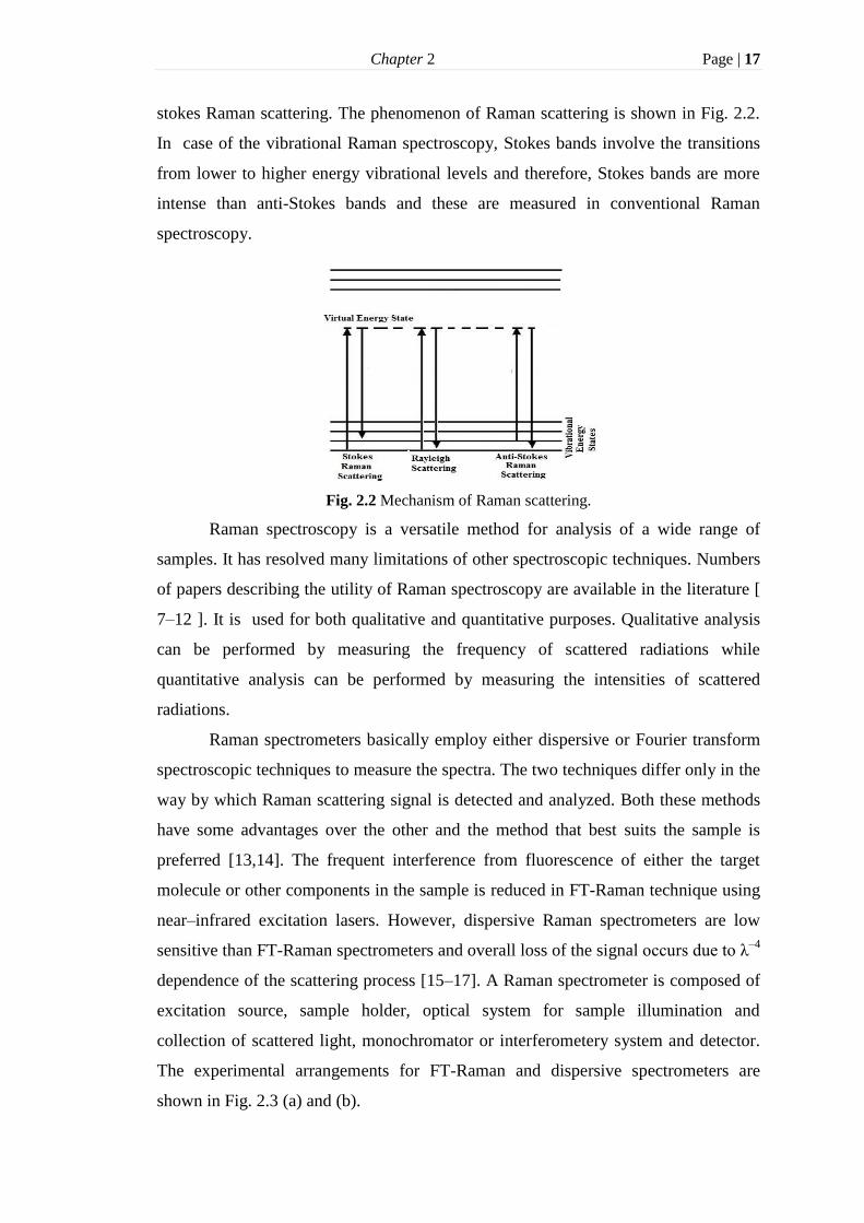
stokes Raman scattering. The phenomenon of Raman scattering is shown in Fig. 2.2.

In case of the vibrational Raman spectroscopy, Stokes bands involve the transitions

from lower to higher energy vibrational levels and therefore, Stokes bands are more

intense than anti-Stokes bands and these are measured in conventional Raman

spectroscopy.

Fig. 2.2 Mechanism of Raman scattering.

Raman spectroscopy is a versatile method for analysis of a wide range of

samples. It has resolved many limitations of other spectroscopic techniques. Numbers

of papers describing the utility of Raman spectroscopy are available in the literature [

7–12 ]. It is used for both qualitative and quantitative purposes. Qualitative analysis

can be performed by measuring the frequency of scattered radiations while

quantitative analysis can be performed by measuring the intensities of scattered

radiations.

Raman spectrometers basically employ either dispersive or Fourier transform

spectroscopic techniques to measure the spectra. The two techniques differ only in the

way by which Raman scattering signal is detected and analyzed. Both these methods

have some advantages over the other and the method that best suits the sample is

preferred [13,14]. The frequent interference from fluorescence of either the target

molecule or other components in the sample is reduced in FT-Raman technique using

near–infrared excitation lasers. However, dispersive Raman spectrometers are low

sensitive than FT-Raman spectrometers and overall loss of the signal occurs due to λ–4

dependence of the scattering process [15–17]. A Raman spectrometer is composed of

excitation source, sample holder, optical system for sample illumination and

collection of scattered light, monochromator or interferometery system and detector.

The experimental arrangements for FT-Raman and dispersive spectrometers are

shown in Fig. 2.3 (a) and (b).

Chapter 2 Page | 18

(a)

(b) Fig. 2.3 Layout of (a) FT-Raman and (b) dispersive Raman spectrometer.

Since Raman scattering is a weak effect, the excitation source should be highly

intense. The intensities of the Raman lines are related to the forth power of the

frequency of the laser and the square of the polarizibility of the molecule. The UV

radiation has higher frequency. It produces less fluorescence but it can degrade the

sample. The choice of the laser depends on the situation. The laser sources like argon

ion (488.0 and 514.5 nm), krypton ion (530.9 and 647.1 nm), He:Ne (632.8 nm),

Nd:YAG (1064 nm and 532 nm) and diode laser (630 and 780 nm) are used as

excitation sources. The laser power incident on the sample is selected in between 10

and 1000 mW. The laser may be continuous or quasi-continuous. Nd:YAG (1064 nm)

laser source is generally preferred due to its lower fluorescent effect than visible

wavelength lasers [18]. A severe limitation of Raman spectroscopy is the fluorescence

phenomenon which is 107 times stronger than Raman scattering. A small amount of

impurities can give strong fluorescence so that it is impossible to detect the Raman

spectrum of the molecule of interest. To avoid masking of Raman scattering by

fluorescence, NIR excitation is preferred, because there are very few electronic

transitions in the NIR. The disadvantage of NIR excitation is that it reduces the

Raman scattering intensity [19].

Chapter 2 Page | 19

The 90º and 180º scattering geometries are used in collecting Raman

scattering and both the arrangements are effective. In the 180º scattering system, the

laser is delivered through the collection lens and the scattered light is collected back

through same lens [20].

The Rayleigh scattering is avoided by using a notch filter in the

interferometery system. The scattered light is collected with a low f-number lens. The

single monochromator should not be used for the Raman measurement because stray

light is not reduced to desired level in it. Therefore, double or triple monochromater is

preferred. The commonly used double monochromator mounting is Czerny-Turner

arrangement. The triple monochromators are suitable for the measurement of low

frequency bands near Rayleigh line. The first monochromator mainly separates the

frequency-shifted Raman scattering from the other radiation and the second

monochromator increases the dispersion and separates the Raman peaks. Triple

monochromators in additive mode have high angular dispersion and permit the

recording of Raman spectra with very good resolution [19].

Detectors are important parts of Raman spectrometers due to the low intensity

of Raman bands. In earlier days, the photographic plate was used as a detector to

record the Raman spectra. Advances in the instrumentation and technology replaced

this detector with more sensitive photomultipliers, image intensifiers and optical

multichannel analyzers. These have greatly enhanced the detection sensitivity.

Photomultiplier has good characteristics in the ultraviolet and visible spectral regions,

hence they are the preferred detectors in a single channel dispersive Raman

spectrometer. The sensitivity of photomultipliers is limited by their dark current

which decreases with decreasing temperature. For routine Raman experiments, Peltier

cooling is often sufficient. Instrumentation such as optical multichannel analyzers or

charge-coupled device (CCD) arrays allow simultaneous recording of extended

spectral ranges with sensitivities comparable to those of photomultipliers.

Multichannel detection at the single photon level is achieved with a back-illuminated

CCD. CCD's are characterized by a high dynamic range (≤100 dB), high quantum

efficiency (90%), wide spectral range (350–900 nm) and low read-out noise (4-6 e-).

Commercial Fourier Transform-Raman spectrometers (FT-Raman) were

introduced in late 1980’s. FT-Raman spectrometer uses a Michelson interferometer

and continuous wave laser such as Nd–YAG. FT-Raman spectra are commonly

measured in a 90◦ scattering geometry. Commercial systems use a Nd:YAG laser

Chapter 2 Page | 20

(1.064 μm) with a near-infrared interferometer coupled to either a liquid nitrogen

cooled germanium (Ge) or indium gallium arsenide (InGaAs) detector. Lasers with

short pulses are not suitable for Raman spectrometer, because the detectors in Raman

spectrometers are highly sensitive and they get saturation very easily.

In the FT-Raman spectrometer, the scattered radiation is focused on the

entrance port of a conventional FTIR Spectrometer where the internal light source of

absorption FTIR spectroscopy is removed. The analysis of the Raman spectrum is

performed using Fourier transform technique. In a modern instrument, weak and

broad but recognizable spectra can be obtained even with low power and low-cost

lasers. Raman scattering using a Raman microscope with a laser pointer or He-Ne

laser can be recorded.

In fact, all advantages of FTIR spectroscopy, as discussed in the above

section, benefit the Raman analysis. In addition to the multiplex and throughput

advantages, the higher wavenumber accuracy is obtained in the interferometric

method. The FT-Raman technique references the measured frequencies to the

accuracy of frequency of an internal He-Ne laser. Therefore, the absolute frequency

can be determined to better than 0.01 cm-1

and the recorded band positions are

limited by the collection parameters.

FT-Raman spectroscopy has provided a means of measuring the Raman

spectrum of visible absorbers without masking by fluorescence. When using the 1064

nm line of a Nd:YAG laser as an excitation source, the Stokes shifted Raman spectrum

occurs in the near infrared. The Raman frequencies in an FT-Raman spectrometer

have Rayleigh and Tyndall radiation at laser frequency which is up to eight orders of

magnitude more intense than the Raman scattering, hence it can cause saturation or

even cause damage to the detectors. Hence, a filter for filtering out radiation at laser

frequency is an essential component of an FT-Raman spectrometer. The best Rayleigh

filter has a cut-off frequency closer to the exciting laser frequency. Rayleigh filters is

the main limiting factor, preventing application of FT-Raman spectrometers in low

frequency Raman spectroscopy [19].

2.1.3 UV–Vis spectroscopy

The absorption of electromagnetic radiation in the UV–Vis region causes a change in

the electronic states of molecules. Molecules having electrons in the delocalised

aromatic systems often absorb in the wavelength region 800–200 nm, resulting in

Chapter 2 Page | 21

excitation of valence electrons from the ground electronic state to the excited

electronic state. Ultraviolet spectra are measured by dissolving the sample in a

solvent. The absorption is measured as a function of wavelength. The informations

obtained from any absorption peak are wavelength of the peak maximum, denoted by

λ max, and the intensity of the absorption. The intensity depends on Lambert’s law,

which states that absorbance of a material is directly proportional to the thickness

(path length) and the fraction of the radiation absorbed is independent of the intensity

of the radiation source, and Beer’s law, which states that the absorption is

proportional to the number of absorbing molecules. For a given ideal solution, there is

a linear relationship between concentration and absorbance provided that the path

length is kept constant; molar extinction coefficient (ε) is constant for each

wavelength.

where, c is the molar concentration and l is the path length in cm, Io is the intensity of

radiation before entering the sample and I is the intensity after leaving the sample

[21,22]. The experimental layout of UV–Vis spectrophotometer is shown in Fig. 2.4.

The radiation sources are a deuterium lamp, which emits light in the UV

region and a tungsten–halogen lamp for the visible region. After passing through a

monochromator, the light is focused on two separate cuvettes inside the sample

chamber. One of the cuvetts contains only the solvent and acts as a reference while

the another one contains sample dissolved in the solvent. The commonly used

detector is a photomultiplier tube (PMT). The light intensity measured by the detector

is converted by it into an electrical signal and is plotted as a function of wavelength.

However, for molecules, vibrational and rotational energy levels are superimposed on

the electronic energy levels. Therefore, the electronic bands are broad as many

transitions with different energies can occur. The broadening is even greater in

solutions owing to solvent-solute interactions [23].

Chapter 2 Page | 22

Fig. 2.4 Layout of UV–Vis Spectrophotometer.

2.2 Theoretical methods

The molecular simulation using the advanced quantum chemical methods is an

exciting field of research in many disciplines like physics, chemistry, biology,

biochemistry, biotechnology, etc. The primary focus of the quantum chemical

calculations is the prediction of structures having minimum energy and other

molecular properties. The calculations are performed taking different parameters into

account which are based on the fundamental laws of physics. The ab initio treatments

of polyatomic molecules consist of Hartree−Fock (HF) method, which excludes

electron correlation, and post Hartree−Fock methods like Moller–Plesset perturbation

(MPn), coupled-cluster (CC), multi−configuration self–consistence field (MCSCF)

and configuration interaction (CI), which include electron correlation [24,25]. These,

however, are the most computationally demanding and restrict the size of the

molecules. These calculations are based upon the basic laws of quantum mechanics

and exploit a variety of mathematical transformation and approximation techniques to

solve the fundamental equations [26]. The density functional theory (DFT) methods

take the effect of electron correlation into account by using exchange−correlation

functionals and attempt to calculate the ground state electron density rather than

molecular wave function and calculate the molecular energy functional. Presently,

DFT is most popular and successful approach to compute properties of medium to

Chapter 2 Page | 23

large sized molecular systems because of its high accuracy and relatively low

computational cost. These theoretical calculations have gained popularity amongst the

scientific community due to the advancement in theoretical models, computer

hardwares and softwares.

2.2.1 Hartree–Fock method

Hartree and Fock proposed ab initio approach to solve the Schrodinger equation by

invoking variational principle for many electron systems. The many-electron

Schrodinger equation is broken into many simpler one-electron equations. Each one

electron equation is solved to yield a single-electron wave function (called an orbital)

and an energy (called an orbital energy). The orbital describes the behaviour of an

electron in the net field of all the other electrons. The equations are solved using an

iteration procedure that gives rise to self−consistence field (SCF) method which uses

mean field, non−relativistic, Born−Oppenheimer and molecular orbital

approximations to solve fundamental equation. According to Born−Oppenheimer

approximation, the nuclei of the molecules are treated as stationary and produce a

static potential field in which electrons are moving. HF method assumes that the

electrons, which are moving in static potential, are not interacting to each other. In

this method, the primary approximation (central field approximation) is that the

Coulombic electron–electron repulsion is taken into account by integrating the

repulsion term. This gives the average effect of the repulsion but not the explicit

repulsion interaction.

Any problem in the electronic structure is solved by time dependent

Schrodinger equation. However, in most cases, while dealing with atoms and

molecules, time independent interactions are taken into account, which is given by

where, is the electronic energy and is the wave function, the Hamiltonian

operator is given by [27].

Chapter 2 Page | 24

where, 1st term is the kinetic energy operator, 2

nd, 3

rd and 4

th terms represent all

possible interactions (potential energies) between charged particles.

For a given system, equation has many independent solutions with

eigenfunctions and eigenvalues . is always taken to be normalized and

orthogonal i.e.

=1 for k=l and 0 otherwise. The average of many measurements of energy is

given by:

Since, each measurement gives one particular eigenvalue of Ĥ, we have;

Equation is the variational principle which states that the energy computed from

a trial wavefunction is always an upper bound to the true ground-state energy.

Thus, one can use the iteration procedure for finding the set of coefficients that

minimize the energy of the resultant wavefunction. The general idea is that the lower

the energy, the better the trial wavefunction.

Molecular orbitals (MOs) can be written as linear combinations of

pre−defined set of one−electron functions known as basis functions or basis sets.

These basis functions are usually centred on the atomic nuclei and so resemblance to

atomic orbitals. The wave function describing each molecular orbital can be expressed

as follows:

where, the coefficients are known as the molecular orbital expansion coefficients

and N is the number of basis functions. The function refers to a trial basis function

and thus represents a trial MO. The are also chosen to be normalized.

According to the Pauli exclusion principle, no two electrons can occupy the

same spin orbital. Therefore, two electrons satisfying the antisymmetry principle can

have same spatial orbital but must differ in spin functions. The antisymmetry is

necessary due to the fermionic character of electrons. For a system having even

number of electrons, restricted Hartree-Fock, (RHF) method is taken into

Chapter 2 Page | 25

consideration. N orbitals are compromised of N/2 orbitals of the form

and N/2 orbitals of the form , where represents the spatial orbital

and and are the spin functions [27]:

The expectation values of the energy form equation (2.7) are obtained by putting

normalization integral =1. It is expressed as

where,

, and are the coulomb and

exchange integrals and is the electron electron repulsion energy. The

Hartree-Fock equations are then given by

where, is a matrix consisting of Lagrange multipliers.

2.2.2 Moller–Plesset perturbation theory

The Moller-Plesset (MP) perturbation theory was proposed in 1934. This theory

provides a systematic approach to calculate the correlation energy of molecular

systems. However, these calculations are not variational. Therefore, the results are not

in general an upper-bound of the true ground state energy. The zero order

(unpertubed) Hamiltionian is defined as the sum of all the N one-electron

Hartree-Fock Hamiltoninas ( ) [28]:

The first-order perturbation is then given by

Chapter 2 Page | 26

where, is the true molecular Hamiltonian (equation (2.5)). The HF energy

associated with the normalized ground state wavefunction is written as

where, is the zero order HF energy and is the first order HF energy. The first

order correction to the ground state energy due to electron correlation in an electronic

system is given by second order perturbation theory (MP2), which can be written as

The Moller-Plesset calculation up to second order is called MP2 method, whereas

higher order corrections are called as MP3, MP4 and so on [29–32]. These

calculations are not applicable to excited states and are also to be used with a higher

basis set for useful results [33]. Correlated models are, however, very useful for

reliable thermodynamic information.

2.2.3 Density functional theory

Density functional theory (DFT) is an important quantum mechanical approach to

calculate the properties of molecular systems by the inclusion of electron density,

, where,

Since, density is a function of wavefunction (functional), the probability of finding

an electron within a volume element in an electron system with arbitrary spin is

given by

Here, the integral is solved over the spin coordinates of all electrons and overall but

one of the spatial orbitals. The electron density is observable unlike the wavefunction

and can be measured experimentally. Therefore, electron density is more attractive

and effective in explaining the molecular properties. The ground state properties of a

molecular system are functionals of the electron density and it is the basic of modern

DFT. The concept was introduced by Hohenberg and Kohen in 1964 [34,35]. The

Chapter 2 Page | 27

ground state energy of a molecule is at minimum if the density corresponds to the

exact density of the ground state, however, the exact form of the energy functional is

not known. Therefore, some approximations are needed. These approximations

include the functional dealing with the kinetic, exchange and correlation energies of

the system of electrons.

According to Hohenberg and Kohn, the ground state properties of a system

can be calculated from the ground state density which in turn can be calculated using

the variational method involving density only.

The ground state properties of an electronic system are a result of the position

of the nuclei. If is the external potential due to the nuclei, the kinetic energy of

the electrons, electron-electron interaction in the Hamiltonian and the electron density

adjust themselves to give the possible minimum energy of the system. Hence, is

the only variable term and is determined by ρ, which determines the number of

electrons:

Therefore, the total density replaces , which describes ground state properties and

state of the system. Hence, the energy can be respectively written as the sum of the

kinetic energy of electrons, interaction energy between them and the energy

corresponding to the external potential:

For a trial density , such that and ,

where, is the energy functional. Each trial density defines a Hamiltonian .

From the Hamiltonian, the wavefunction for the ground state can be derived. This

wavefunction will not be a ground state for the Hamiltonian of the real system:

where, is the true ground state density of the real system. The condition of

minimum energy functional is then given by:

Although the Hohenberg Kohn method provides minimized energy of a system, the

kinetic energy is not known with a satisfactory level of accuracy. Kohn and Sham

proposed a method to determine the kinetic energy by combining wavefunctions and

Chapter 2 Page | 28

the density approach. According to Kohn and Sham, the energy functional can be

written as

where, is the kinetic energy of electrons in a system which has the same density

ρ as the real system (non interacting electrons); is the exchange-correlation

energy; is the pure coulomb interaction between electrons given by equation

The exchange energy arises due to the antisymmetry of the wavefunction while

correlation effects are because of the dynamic correlation in the motion of individual

electrons [24]. The effective potential is then given by:

where, =

is the external potential, the potential reflected from the

nuclei. The exchange correlation potential is defined as:

The Schrodinger equation for non interacting particles moving in external potential

is given as:

(2.29)

The Kohn Sham (KS) operator,

depends only upon and the KS

orbitals are used to calculate the total density given by:

Although, KS DFT method gives good results for the medium to large molecular

systems but has some drawbacks also because of the approximate functional [30]. The

exchange correlation functionals include local spin density aproximation (LSDA),

generalized gradient approximation functional (GGA), meta-GGA and hybrid

functionals. The LSDA functionals assume slowly varying uniform electron density

of the system. GGA approximation accounts for the non uniformity of the electron

density and corrects the local density approximation through an additional density

Chapter 2 Page | 29

gradient correction, which makes the functional more flexible. Some commonly used

GGA exchange functionals are Perdew and Wang's (PW86, PW91) [36,37] and

Becke's (B88) [38]. The meta-GGA functional modifies GGA by approximating the

kinetic energy density. In the present thesis, Beck's 3 exchange and Lee-Yang-Par

(B3LYP) hybrid correlation functional, the most widely used exchange−correlation

functional within DFT calculations on molecules, has been used due to its accuracy.

The B3LYP functional is defined as [39,40]

where, uses HF theory and a's are constants (empirical parameters).

2.2.4 Time dependent density functional theory

Despite its popularity, DFT being a static ground state theory, is not appropriate for

handling time dependent phenomena or excited states. Time dependent density

functional theory (TD-DFT) is one of the widely used simulation approach and

extends the basic ideas of ground state DFT to the treatment of excitations or more

general time dependant phenomenon. The time-dependant analogous of DFT (TD-

DFT) was presented by Runge and Gross in 1984 [41] and the development of

effective linear-response formalism by Casida leads to a rapid and efficient solution of

TD-DFT equations for molecules [42]. TD-DFT shows that there is a one-to-one

correspondence between time-dependent density and time-dependent

potentials for a given initial condition. By virtue of the one-to-one

correspondence of potential and density, we can take the density of KS non-

interacting electrons to be same as the interacting density of the original system. The

time dependent KS electrons obey the time-dependent Schrodinger equation:

where,

is the Kohn-Sham Hamiltonian. The density

of the non-interacting system can be calculated from the Kohn-Sham orbitals:

The time dependent Kohn-Sham potential is given by

Chapter 2 Page | 30

The first term is the external potential, whereas the second accounts for the

classical electrostatic interaction between the electrons. The third term, the

potential has an essentially functional dependence on the density, includes all

nontrivial many-body effects. The potential at time and position depends on the

density at all other positions and all previous times. The final results depends upon the

quality of approximation of , the only fundamental approximation in TD-DFT.

is not only a functional of density, but it also depends on the initial Kohn-Sham

determinant and on the initial many-body wave function, which is always neglected

for practical reasons. Explicit density functionals, like the adiabatic LDA, only retain

the density dependence [43].

2.2.5 Basis set

Basis sets constitute an essential component of the quantum chemical calculations to

describe the molecular electronic structure. They provide a best mathematical

description of the unknown molecular orbitals with a minimum possible

computational cost. A large number of basis sets have been proposed over the years.

The general expression for a basis function is given by

where, is the normalization constant, is the orbital exponent and r is the distance

from origin where the nucleus is located. It was John C. Slater who first turned to

orbital computation using basis sets. These basis sets are known as Slater type

orbitals (STOs). The STOs are defined as

where, are spherical coordinates, is the angular momentum part which

describes the shape and are quantum numbers.

In 1950, Boys suggested Gaussian type functions (GTOs), which contain the

exponential , rather than of the STOs and are easy to calculate. However,

they neither represent the electron density nor the STOs. Therefore, each basis

function consists of linear combination of several GTOs with fixed coefficients.

GTO(3G) function can be defend as

Chapter 2 Page | 31

where, the three values of and are fixed and that number is included in the

designation. The difference between STOs and GTOs is that the pre-exponential

factor in STO function is dropped in the GTO function, which restricts single

Gaussian primitives for each principal quantum level. The exponential factor in GTO

is squared and the angular momentum factor is made into a simple function of

Cartesian coordinates.

Minimal basis sets are represented in the form STO-nG, where, n denotes the

number of primitive GTOs (G) used to approximate one STO for each inner and

valence shell. They include STO-3G, STO-4G, STO-6G and the polarized version of

STO-3G (STO-3G*). The individual GTOs are called primitive orbitals. A group of

several GTOs form contracted Gaussian functions. STO-3G consists of three

primitive Gaussians in each basis function.

Split valence basis sets include 3-21G, 3-21G* (polarized), 3-21+G (diffuse),

3-21+G* (polarized and diffuse), 6-31G, 6-31G*, 6-31+G

*, 6-31G(3df,3pd), 6-311G,

6-311G*, 6-311+G

* etc.

These basis sets use one function for orbitals that are not in

the valence shell and two functions for those in the valence shell. 3-21G is the

smallest split valence basis set, which uses three primitive expansion for the 1s orbital

and splits the valence orbitals into a two basis function. The inner function is a

contraction of two Gaussians and the outer function is a single Gaussian. The double

zeta basis set, considered as a general split valence basis set, uses two basis functions

for each atomic orbital and each basis function is a contraction of small set of

primitives. The triple zeta basis set uses three basis functions [44–46].

The 6-311G basis set is having triple zeta quality in the valence part and only

minimal in the core. The flexibility of this basis set in the valence region of the

molecule is increased by adding polarization functions. These functions have a set of

Gaussian functions one unit higher in angular momentum than the Gaussian functions

present in the ground state of the atom. The polarization functions are denoted by

single (*) or double (**) asterisk or by (d,p). A single * or d denotes that polarization

has been taken into account in the non-hydrogen atoms, whereas, ** or (d,p)

represents that both hydrogen and non-hydrogen atoms are taken into account.

To account for the electron density over a large region for an atom in an

anion, excited or Rydberg states and lone pair of electrons, diffuse functions are

usually preferred. These are represented by + or ++, where + denotes the sp-type

Chapter 2 Page | 32

diffuse basis functions added to non-hydrogen atoms and ++ indicates the

consideration of one set of sp- and s-type diffuse functions to non-hydrogen and

hydrogen atoms respectively.

2.2.6 Geometry optimization

The optimization of geometry plays an important role in the quantum chemical studies

concerned with the structure determination or reactivity of molecules. The location of

the atoms specify the structure of a molecule. For a given structure and electronic

state, a molecule has a specific energy. By virtue of Born−Oppenheimer, the energy

of a molecule can be described as a function of fixed nuclear positions. The variation

of energy as function of the structure of a molecule is given by potential energy

surface (PES),which can be visualized as a hilly landscape where the minimum

energy position represents the equilibrium structure. The transition state structure is

also represented in this PES. The procedure of locating stationery points (minima or

maxima) on the PES for calculating geometry and energy of a molecule is called as

geometry optimization. The efficient methods to find a local minimum require a

repeated calculation of U (molecular electronic energy including inter-nuclear

repulsions) and its gradient (3N-6 partial derivatives) [47]. For a structure to be

characterized as minimum, the gradient must be zero and all the eigen values of the

Hessian (matrix of second derivatives of energy, also known as Force constant

matrix) corresponding to molecular vibrations must be positive. A transition state has

a zero gradient and a Hessian that has only one negative eigen value (imaginary

frequency). The performance of any geometry optimization can be improved by

choosing a good coordinate system. The presence of very stiff and flexible

coordinates, strong coupling between coordinates and other neighbouring coordinates

and anharmonicity can slow down an optimization process [47]. Cartesian coordinates

are the most universal and least ambiguous. However, they do not reflect the chemical

structure and bonding of a molecule. The x, y and z coordinates are also coupled to

each other and the surrounding coordinates of the atoms. Therefore, they are not well

suited in optimization. Being more descriptive of the molecular structure, internal

coordinates such as bond lengths and valence angles are however useful for

optimization of the geometry. The coupling between stretches, bends and torsions are

usually much smaller than in Cartesian coordinates. The combination of all bonds,

angles and torsions (primitive redundant coordinate system) represent the intrinsic

Chapter 2 Page | 33

connectivity and flexibility of cyclic molecules. However, such a coordinate system

leads to sacking of geometrical parameters for the cyclic ones. Therefore, certain

combinations of redundant internals need to be constrained during optimization [48–

50].

2.2.7 Vibrational frequency calculations

The interpretation and correct assignment of the vibrational spectra of larger

polyatomic molecules is virtually impossible without quantum-mechanical

calculations. The computations of the vibrational frequencies are also essential to

classify a stationery point as a local minimum or an nth order saddle point on the PES

[30]. The vibrational frequencies are computed analytically from the optimized

structure of a molecule by evaluating the Hessian or force constant matrix. The set

containing 3N linear equations in 3N unknowns is solved:

where, is the Kronecker delta, and are unknown parameters. is the

mass weighted force constant matrix. For a nontrivial solution, the determinant of

equation (2.36), which is of order 3N, must be zero:

λ

This determinant can be expended in polynomial form whose highest power of

is

with 3N roots for . The vibrational harmonic frequencies are obtained from

relation:

The vibrational transitions in which the vibrational quantum number goes

from 0 to 1 with no change in other quantum numbers are called the fundamental

frequencies. These fundamental frequencies incorporate anharmonic corrections and

are generally smaller than the harmonic frequencies. In order to account for the

anharmonicity, effective corrections using empirical scaling factors are reported at

various levels of theory, although they are not appropriate for all vibrational modes

[51–58]. The overtone and combination bands are also not predicted using harmonic

approximation. Therefore, to overcome these limitations of harmonic approximation,

several anharmonic approaches have been proposed to account for the anharmonicity.

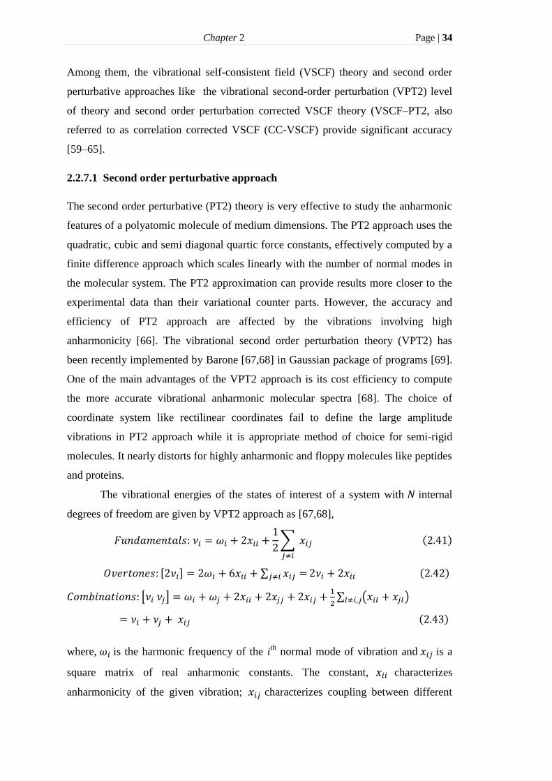
Chapter 2 Page | 34

Among them, the vibrational self-consistent field (VSCF) theory and second order

perturbative approaches like the vibrational second-order perturbation (VPT2) level

of theory and second order perturbation corrected VSCF theory (VSCF–PT2, also

referred to as correlation corrected VSCF (CC-VSCF) provide significant accuracy

[59–65].

2.2.7.1 Second order perturbative approach

The second order perturbative (PT2) theory is very effective to study the anharmonic

features of a polyatomic molecule of medium dimensions. The PT2 approach uses the

quadratic, cubic and semi diagonal quartic force constants, effectively computed by a

finite difference approach which scales linearly with the number of normal modes in

the molecular system. The PT2 approximation can provide results more closer to the

experimental data than their variational counter parts. However, the accuracy and

efficiency of PT2 approach are affected by the vibrations involving high

anharmonicity [66]. The vibrational second order perturbation theory (VPT2) has

been recently implemented by Barone [67,68] in Gaussian package of programs [69].

One of the main advantages of the VPT2 approach is its cost efficiency to compute

the more accurate vibrational anharmonic molecular spectra [68]. The choice of

coordinate system like rectilinear coordinates fail to define the large amplitude

vibrations in PT2 approach while it is appropriate method of choice for semi-rigid

molecules. It nearly distorts for highly anharmonic and floppy molecules like peptides

and proteins.

The vibrational energies of the states of interest of a system with internal

degrees of freedom are given by VPT2 approach as [67,68],

where, is the harmonic frequency of the ith

normal mode of vibration and is a

square matrix of real anharmonic constants. The constant, characterizes

anharmonicity of the given vibration; characterizes coupling between different

Chapter 2 Page | 35

normal modes resulting from anharmonicity and are determined from cubic and

quartic force constants.

2.2.7.2 Vibrational self−consistent field approach

The VSCF method is equivalent to the Hartree method used for many electron

systems. The method, developed by Bowman, Carney, Cohen, Gerber and Ratner in

late 1970s, is employed to account for the anharmonicity in molecules [70–73]. In this

approximation, each vibrational mode is characterized by moving in the mean field of

the rest of vibrational motions and the wavefunctions corresponding to different

vibrational modes are determined using a self-consistent method. The total vibrational

wavefunction is then written as a product of each normal mode wavefunctions. This

method is equivalent to Hartree method for many electron systems and has been

successfully used for small to medium sized molecules [74–78]. The major challenge

for this approximation is the calculation of multidimensional potentials which depend

on its typical mathematical form [79]. The VSCF potential is given by the adding one-

mode, two-mode, three-mode terms and so on in mass weighted normal coordinate Q

[79]:

where, the first term represents the harmonic potential and the intrinsic anharmonicity

of the potential function along the normal coordinates (diagonal approximation); the

second term consists of pair-wise coupling between different normal modes, etc. The

VSCF energy is then given by the self consistency approach as:

where, first term is the sum of all individual mode energies and the other terms

accounts for the double counting of the interactions in the energy calculation. The

accuracy of the VSCF approximation depends strongly on the choice of coordinates

which can best reproduce the mutual separability for VSCF approximation [66]. The

normal coordinate system often fails for soft torsional motions. The curvilinear

Chapter 2 Page | 36

internal coordinates offer a good accuracy over the normal coordinates representation

of VSCF. The second order perturbation corrected VSCF, PT2-VSCF (CC–VSCF), an

important variant of VSCF, was introduced by Gerber and co-workers that improves

the VSCF energies, keeping the computational cost in control for relatively large

molecules. The total energy for the CC−VSCF approximation is given by:

where,

where, is the effective potential for mode i corresponding to is the

difference between the correct Hamiltonian and VSCF one (perturbation) which must

be small.

2.2.7.3 Quartic force field potential and anharmonic mode-mode coupling

strength

The potential energy surface of a molecule consisting of N atoms is given by Taylor

expansion as [80].

where, , , and denote the potential energy and its second, third and

fourth order derivatives respectively and is the normal coordinate at the equilibrium

structure. The third and fourth order energy derivatives can be obtained through

numerical differentiation, while the higher order terms are neglected. Yagi and et. al.

[80] developed a method to determine the expansion coefficient in the above equation

energy derivatives calculated by an ab initio electronic structure method (least square

fit method) at the equilibrium structure. In the two mode coupling representation of

the quartic force field (2MR-QFF), which can be constructed with less computational

effort than direct VSCF calculations, can be written as:

Chapter 2 Page | 37

where,

Similarly n-mode coupling representation quartic force field (nMR-QFF) can be

determined from equation (2.46).

Anharmonic interactions are of two types: (1) intrinsic anharmonicity of the

mode and (2) anharmonic mode-mode coupling. Therefore, the potential function,

, in the 2MR-QFF approximation can be written as described in

equation (2.42) upto two terms and neglecting the higher order terms. The

contribution of the intrinsic anharmonicity in a mode is given by [81]

The contribution of anharmonic mode pair coupling is given by

where, is the frequency. The detection of the mode coupling strengths is important

in solving the vibrational Schrodinger equation and in generating a PES. The mode

coupling strengths based on QFF coefficients can be potentially used to detect the

strong coupling and discard terms that need not to be computed in generating a PES.

The mode coupling strength based on 2MR-QFF for the ground state is given by

The coefficient is obtained by numerical differentiations of the analytical

Hessian.

Chapter 2 Page | 38

References

[1]. C. Berthomieu, R. Hienerwadel, Photosynth. Res. 101 (2009) 157–170.

[2]. B.H. Stuart, Infrared Spectroscopy: Fundamentals and Applications, John

Wiley & Sons, England, 2004.

[3]. B.H. Stuart, Infrared Spectroscopy of Biological Applications: An Overview,

Encyclopedia of Analytical Chemistry, John Wiley & Sons, Ltd. 2012.

[4]. P.R. Griffiths, J.A. De Haseth, Fourier Transform Infrared Spectrometry, John

Wiley & Sons, New York, 1986.

[5]. R.S. Brettzlaff, T.B. Bahder, Rev. Phys. Appl. 21 (1986) 833–844.

[6]. C.V. Raman, K.S. Krishnan, Nature 121 (1928) 501–502.

[7]. W. Kiefer, V. Pfeufer, P. Vogt, Spectroscopy 27 (2012) 28–35.

[8]. W. Kiefer, J. Raman. Spectrosc. 38 (2007) 1538–1553.

[9]. W. Kiefer, J. Raman. Spectrosc. 39 (2008) 1710–1725.

[10]. W. Kiefer, J. Raman. Spectrosc. 40 (2009) 1766–1779.

[11]. J. Popp, W. Kiefer, Encyclopedia of Analytical Chemistry, John Wiley & Sons

Ltd, Chichester, 2000.

[12]. G.S. Bumbrah, R.M. Sharma, Egypt. J. Forensic Sci. (2015),

http://dx.doi.org/10.1016/j.ejfs.2015.06.001

[13]. Y. Wang, R.L. McCreery, Anal. Chem. 61 (1989) 2647–2651.

[14]. R.S. Dass, Y.K. Agarwal, Vib. Spectrosc. 57 (2011) 163–176.

[15]. P. Hendra, C. Jones, G. Warnes, Fourier Transform Raman Spectroscopy:

Instrumentation and Chemical Applications, Ellis Horwood Ltd, 1991.

[16]. D.B. Chase, J.F. Rabolt, Fourier Transform Raman Spectroscopy: From

Concept to Experiment, Academic Press, New York, 1994.

[17]. I.R. Lewis, H.G.M. Edwards, Handbook of Raman Spectroscopy: From the

Research Laboratory to the Process Line, Marcel Dekker, Inc, 2001.

[18]. J.R. Ferraro, K. Nakamoto, Introductory Raman Spectroscopy, 2nd

edition,

Academic Press, Boston, 1994.

[19]. G. Gauglitz, T. Vo-Dinh, Handbook of Spectroscopy, Wiley-VCH Verlag

GmbH & Co. KGaA, Weinheim, 2003.

[20]. E. Smith, G. Dent. Modern Raman Spectroscopy: A Practical Approach, John

Wiley & Sons, Ltd. 2005.

Chapter 2 Page | 39

[21]. S.L. Upstone, Ultraviolet/Visible Light Absorption Spectrophotometry in

Clinical Chemistry, Encyclopedia of Analytical Chemistry, John Wiley &

Sons, Ltd. Chichester, 2000.

[22]. T. Owen, Fundamentals of UV-Vis Spectroscopy, Hewlett-Packard Company,

Germany, 1996.

[23]. D. Whittaker, Interpreting Organic Spectra, The Royal Society of Chemistry,

2000.

[24]. C. Moller, M.S. Plesset, Phys. Rev. 46 (1934) 618−622.

[25]. J.A. Pople, M.H. Gordon, K. Raghavachari, J. Chem. Phys. 87 (1987)

5968−5975.

[26]. J.B. Foresman, A. Frisch, Exploring Chemistry with Electronic Structure

Methods, 2nd edition, Gaussian, Inc, Pittsburgh, 1996.

[27]. R.G. Parr, W. Yang, Density-Functional Theory of Atoms and Molecules,

Oxford University Press, New York, 1989.

[28]. M. Mueller, Fundamentals of Quantum Chemistry, Kluwer Academic

Publishers, New York, 2002.

[29]. P. Atkins, R. Friedman, Molecular Quantum Mechanics, 4th

edition, Oxford

University Press Inc., New York, 2005.

[30]. I.N. Levine, Quantum Chemistry, 6th

edition, PHI Learning Private Ltd., New

Delhi, 2010.

[31]. C.J. Cramer, Essentials of Computational Chemistry: Theories and Models,

2nd

edition, John Wiley & Sons, Ltd., England, 2004.

[32]. H.B. Schlegel, J. Comp. Chem. 3 (1982) 214−218.

[33]. K.I. Ramachandran, G. Deepa, K. Namboori, Computational Chemistry and

Molecular Modelling: Principles and Applications, Springer, Verlag Berlin

Heidelberg, 2008.

[34]. P. Hohenberg, W. Kohn, Phys. Rev. B 136 (1964) 864−871.

[35]. W. Kohn, Rev. Mod. Phys. 71 (1999) 1253−1266.

[36]. J.P. Perdew, J.A. Chevary, S.H. Vosko, K.A. Jackson, M.R. Pederson, D.J.

Singh, C. Fiolhais, Phys. Rev. B 46 (1992) 6671−6687.

[37]. J.P. Perdew, W. Yue, Phys. Rev. B 33 (1986) 8800−8802.

[38]. A.D. Becke, Phys. Rev. A 38 (1988) 3098−3100.

[39]. C. Lee, W. Yang, R.G. Parr, Phys. Rev. B 37 (1988) 785−789.

[40]. A.D. Becke, J. Chem. Phys. 98 (1993) 5648−5652.

Chapter 2 Page | 40

[41]. E. Runge, E.K.U. Gross, Phys. Rev. Lett. 52 (1984) 997–1000.

[42]. M.E. Casida, Recent Advances in Density Functional Methods, World

Scientific, Singapore, 1995.

[43]. M.A.L. Marques, E.K.U. Gross, Annu. Rev. Phys. Chem. 55 (2004) 427–455.

[44]. R. Poirier, R. Kari, I.G. Csizmadia, Handbook of Gaussian Basis Sets,

Elsevier, New York, 2007.

[45]. T.H. Dunning, Jr., J. Chem. Phys. 90 (1989) 1007−1023.

[46]. D.E. Woon, T.H. Dunning Jr., J. Chem. Phys. 98 (1993) 1358−1371.

[47]. H.B. Schlegel, WIREs Comput. Mol. Sci. 1 (2011) 790–809.

[48]. P. Pulay, G. Fogarasi, J. Chem. Phys. 96 (1992) 2856–2860.

[49]. J. Baker, A. Kessi B. Delley, J. Chem. Phys. 105 (1996) 192–212.

[50]. O. Farkas, H.B. Schlegel, J. Chem. Phys. 109 (1998) 7100–7104.

[51]. M.P Andersson, P.J. Uvdal, Phys. Chem. A 109 (2005) 2937−2941.

[52]. J.P. Merrick, D. Moran, L.J. Radom, Phys. Chem. A 111 (2007)

11683−11700.

[53]. Y. Tantirungrotechai, K. Phanasant, S. Roddecha, P. Surawatanawong, V.

Sutthikhum, J. Limtrakul, J. Mol. Struct. (Theochem) 760 (2006) 189−192.

[54]. M.W. Wong, Chem. Phys. Lett. 256 (1996) 391−399.

[55]. D.J. Defrees, A.D. Mclean, J. Chem. Phys. 82 (1985) 333−341.

[56]. J.A. Pople, A.P. Scott, M.W. Wong, L. Radom, Isr. J. Chem. 33 (1993)

345−350.

[57]. A.P. Scott, L.J. Radom, Phys. Chem. 100 (1996) 16502−16513.

[58]. G. Rauhut, P. Pulay, J. Phys. Chem. 99 (1995) 3093−3100.

[59]. V. Barone, J. Chem. Phys. 122 (2005) 014108−014118.

[60]. J. M. Bowman, J. Chem. Phys. 68 (1978) 608–610.

[61]. G.D. Carney, L.L. Sprandel, C.W. Kern, Adv. Chem. Phys. 37 (1978) 305–

379.

[62]. M. Cohen, S. Greita, R.D. McEarchran, Chem. Phys. Lett. 60 (1979) 445–450.

[63]. R.B. Gerber, M.A. Ratner, Chem. Phys. Lett. 68 (1979) 195–198.

[64]. L.S. Norris, M.A. Ratner, A.E. Roitberg, R.B. Gerber, J. Chem. Phys. 105

(1996) 11261–11267.

[65]. J.O. Jung, R. B. Gerber, J. Chem. Phys. 105 (1996) 10682–10690.

[66]. T. K. Roy, R. B. Gerber, Phys. Chem. Chem. Phys. 15 (2013) 9468−9492.

[67]. V. Barone, J. Chem. Phys. 122 (2005) 014108−014118.

Chapter 2 Page | 41

[68]. V. Barone, M. Biszysko, J. Bloino, Phys. Chem. Chem. Phys.16 (2014) 1759–

1787.

[69]. M.J. Frisch, G.W. Trucks, H.B. Schlegel, G.E. Scuseria, M.A. Robb et. al.,

Gaussian 09, Revision D.01, Gaussian, Inc., Wallingford CT, 2009.

[70]. J. M. Bowman, J. Chem. Phys. 68 (1978) 608–610.

[71]. G.D. Carney, L.L. Sprandel, C.W. Kern, Adv. Chem. Phys. 37 (1978) 305–

379.

[72]. M. Cohen, S. Greita, R.D. McEarchran, Chem. Phys. Lett. 60 (1979) 445–450.

[73]. R.B. Gerber, M.A. Ratner, Chem. Phys. Lett. 68 (1979) 195–198.

[74]. T.K. Roy, T. Carrington Jr., R. B. Gerber, J. Phys. Chem. A, 118 (2014)

6730–6739.

[75]. K. Meng, J. Wang, Phys. Chem. Chem. Phys. 13 (2011) 2001–2013.

[76]. B. Brauer, R.B. Gerber, M. Kabelac, P. Hobza, J.M. Bakker, A.G.A. Riziq,

M.S. de Vries, J. Phys. Chem. A, 109 (2005) 6974–6984.

[77]. L. Pele, R. B. Gerber, J. Chem. Phys. 128, (208) 165105–165115.

[78]. R. Knaanie, J. Sebek, J. Kalinowski, R. B. Gerber, Spectrochim. Acta A 119

(2014) 2–11.

[79]. T.K. Roy, R.Sharma, R. B. Gerber, Phys. Chem. Chem. Phys. 18 (2016)

1607–1614.

[80]. K. Yagi, T. Taketsuga, K. Hirao, M.S. Gordon, J. Chem. Phys. 113 (2005)

1005–1017.

[81]. Y. Miller, G.M. Chaban, R.B. Gerber, J. Phys. Chem. A 109 (2005) 6565–

6574.

3 Quantum chemical calculations and analysis of FTIR, FT-Raman

and UV-Vis spectra of temozolomide molecule

3.1 Introduction

One of the most severe forms of human cancer is glioblastoma, which is a primary

brain tumor [1]. Malignant gliomas (glioblastoma multiforme and anaplastic

astrocytoma) occur more frequently than other types of primary central nervous

system tumours. The media reported survival is less than 1 year even if these cancers

are treated with surgery, radiation and chemotherapy [2]. Temozolomide (TMZ) is an

orally administered alkylating agent, used largely in the therapy of malignant brain

tumours including glioblastoma and astrocytoma, which are serious and aggressive

types of brain cancers [3]. It readily crosses the blood-brain barrier and has a broad

spectrum of antineoplastic activity [4‒6]. The anticancer, antitumor activity and skin

delivery potency of TMZ ester prodrugs have been reported [7,8]. Synthesis and

structural evolution of TiO2 nanostructured reservoir with TMZ are reported [9]. UV

spectrophotometric method has been developed by Razak et. al. for the quantitative

determination of TMZ in bulk and capsule [10]. High-performance liquid

chromatographic analysis is carried out [11]. Some cocrystals of TMZ have been

characterised by XRD, FTIR and FT-Raman analysis [12]. The feasibility of

encapsulating TMZ into polybutylcyanoacrylate nanoparticles by polymerisation is

reported by Xin-Hua et. al. [13]. The physiochemical characteristics of TMZ process-

related impurities and their structure have been studied [14]. Recently, the interaction

between TMZ and water has been reported [15].

Quantum chemical computations have become important in predicting the

molecular structure and properties of biologically important compounds and drugs.

For proper understanding of the vibrational spectra of polyatomic molecules, the

theoretical calculations are invaluable tools for reliable assignments of vibrational

Chapter 3 Page | 44

bands [16–21]. Structural and vibrational parameters predicted by theoretical methods

often depend on the level of the theory, basis set and inclusion of correlation effects.

Harmonic frequency approximation is sometimes useful for rigid molecules, but has

limited accuracy for flexible systems. Vibrational frequencies computed by the usual

harmonic approximation overestimate the observed values partly because of strong

anharmonic character of some vibrations. High frequency modes due to C–H, N–H

and O–H stretching vibrations usually show deviations from experimental data due to

large anharmonicity associated with these vibrations. Therefore, the scaling

procedures are used to obtain better agreement with experimental data [22‒24].

However, in order to avoid the scaling procedure, and to attain good accuracy in the

calculated vibrational spectra of biological molecules, we need to consider

anharmonic treatment.

In this chapter, the FTIR, FT-Raman and UV-Vis spectra of TMZ are

discussed. The optimised molecular geometrical parameters and anharmonic

frequencies of TMZ are calculated using DFT method with 6-311++G(d,p) basis set.

The anharmonic effects in the vibrational spectra are considered by second order

perturbative approach (VPT2). The observed and simulated electronic absorption

spectra are also reported. Natural bond orbital (NBO) analysis, molecular electrostatic

potential (MEP) mapping, HOMO–LUMO analysis, non-linear optical properties

(NLO), and other thermochemical properties of TMZ are also presented.

3.2 Experimental details

The TMZ sample in solid form was obtained from Sigma Aldrich Chemicals, USA

and used as such without further purification to record FTIR, FT-Raman and UV-Vis

spectra. The FTIR spectrum was recorded at room temperature on Bruker Tensor-37

spectrometer in the mid IR region (4000–400 cm-1

) using KBr pellet technique, with a

spectral resolution of 2 cm-1

. To increase the signal-to-noise ratio, a minimum of 32

scans were accumulated. The FT-Raman spectrum in solid phase was recorded at

room temperature on Bruker RFS spectrometer in the region 4000-50 cm-1

, with a

spectral resolution of 2 cm-1

, using 1064 nm line of Nd:YAG laser as excitation

wavelength. The UV-Vis spectrum was recorded in ethanol solvent in the region 800–

200 nm using Lambda-950 UV-Vis-NIR spectrophotometer.

Chapter 3 Page | 45

3.3 Computational details

The theoretical computations for the TMZ molecule were carried out by Gaussian 09

program [25] using DFT level of theory with 6-311++G(d,p) basis set. Electron

correlations in the DFT were included using the Becke's three- parameter hybrid

exchange functional (B3) [26–28] and the Lee Yang Par (LYP) correlation functional

[29]. The optimized geometries were taken as the input structures for calculations of

harmonic and anharmonic vibrational frequencies, IR intensities and Raman activities.

The Raman activity , corresponding to an ith

normal mode , was converted into

intensity Ri by the following relationship [30].

where, is the laser exciting wavenumber; f is a suitably chosen common

normalization factor for all peak intensities; h is the Planck constant; k is the

Boltzmann constant; c and T are the speed of light and temperature (298 Kelvin)

respectively. The anharmonic corrections in the vibrational frequencies of TMZ were

computed using VPT2 approach implemented by Barone, as well as, VSCF/2MR-

QFF and CC-VSCF methods implemented into GAMESS-US package [31]. For the

dimer structures of TMZ, only the harmonic approximation at DFT level of theory

was taken into account. Since, the vibrational spectra not only depend upon the bond

strengths within molecules, but, also on the environments around them. The solvation

methods are therefore, attractive due to their reliability coupled to computational costs

comparable with those of the corresponding computations in gas phase [32].

Therefore, in order to provide an insight into solute-solvent interactions and to figure

out to which extent the calculated results in solvent agree with the experimental

observations, the harmonic and anharmonic frequencies in the monomer structure of

TMZ were also computed in dimethyl sulfoxide (DMSO) using IEF-PCM model [33].

The broadening in the simulated spectra was simulated using Lorentzian line shape

with FWHM as 6 cm-1

. The vibrational spectra have been interpreted by means of

visual inspection of animated modes and potential energy distribution (PED) using

VEDA 4 program [34]. In order to understand the coupling between pair of modes,

the magnitudes of mode-mode coupling for the ground state were estimated. The

2MR-QFF potential energy function was used for calculating anharmonic mode-mode

Chapter 3 Page | 46

coupling strengths [35,36]. The electronic spectrum was simulated using TD-DFT/6-

311++G(d,p) method in combination with IEF-PCM model [32] in ethanol solvent.

Furthermore, the HOMO and LUMO energies were predicted to interpret the orbital

overlapping and the possibility of charge transfer within the molecule. The group

contributions to the HOMO and LUMO orbitals were obtained by Gauss-sum 2.2

program [37]. MEP, NBO, thermodynamic and NLO properties of the title molecule

are also calculated at DFT/-311++G(d,p) level of theory. The NBO analysis was

performed using NBO 3.1 program [38] .

3.4 Results and discussions

3.4.1 Geometric structure

The optimized geometries of TMZ monomer and dimer structures (D1, D2 and D3)

with atom numbering scheme are shown in Fig. 3.1. The molecular energies

corresponding to optimized structures of TMZ monomer are –711.38056344 a.u. in

isolated phase, –711.40082132 a.u. in solvent phase, –1422.781958 a.u. for D1, –

1422.76824930 a.u. for D2 and –1422.76806627 a.u. for D3. Among the dimer

structures, D1 is found energetically more stable. The computed optimized parameters

are given in Table 3.1.

Fig. 3.1 Optimized structures of the monomer and dimer forms of temozolomide.

Chapter 3 Page | 47

Table 3.1

Optimized geometrical parameters of monomer and dimer structures of temozolomide

molecule at DFT/6-311++G(d,p) basis set.

Bond length

(Å)

Monomer

D1

D2

D3

Bond angle

(◦)

Monomer

D1

D2

D3 IEF-

PCM/DMSO

isolated IEF-

PCM/DMSO

isolated

C1‒N11 1.313 1.313 1.312 1.316 1.313 N11‒C1‒N16 110.6 110.7 110.7 110.6 110.7

C1‒N16 1.368 1.367 1.368 1.364 1.367 N11‒C1‒H17 127.0 127.1 127.1 127.0 127.1

C1‒H17 1.078 1.078 1.078 1.078 1.078 N16‒C1‒H17 122.4 122.2 122.2 122.4 122.2

C2‒N12 1.467 1.463 1.463 1.464 1.463 N12‒C2‒H18 109.9 110.1 110.2 110.1 110.1

C2‒H18 1.090 1.091 1.091 1.091 1.091 N12‒C2‒H19 107.0 106.8 106.8 106.8 106.8

C2‒H19 1.086 1.087 1.087 1.087 1.087 N12‒C2‒H20 109.9 110.1 110.2 110.1 110.1

C2‒H20 1.090 1.091 1.091 1.091 1.091 H18‒C2‒H19 110.2 110.3 110.3 110.3 110.3

H3‒N13 1.009 1.008 1.009 1.016 1.008 H18‒C2‒H20 109.6 109.0 109.0 109.0 109.0

H4‒N13 1.008 1.007 1.025 1.008 1.007 H19‒C2‒H20 110.2 110.3 110.3 110.4 110.3

C5‒C8 1.487 1.493 1.492 1.495 1.493 C8‒C5‒C10 128.9 128.8 129.0 127.7 128.8

C5‒C10 1.387 1.387 1.387 1.387 1.387 C8‒C5‒N11 121.9 121.8 121.7 123.2 121.8

C5‒N11 1.374 1.374 1.373 1.374 1.374 C10‒C5‒N11 109.2 109.3 109.3 109.1 109.3

C9‒O6 1.209 1.207 1.207 1.207 1.207 C5‒C8‒O7 122.2 122.6 120.9 121.3 122.6

C8‒O7 1.230 1.218 1.232 1.22 1.218 C5‒C8‒N13 113.9 113.1 114.4 114.5 113.1

C8‒N13 1.351 1.362 1.344 1.358 1.362 O7‒C8‒N13 123.8 124.3 124.7 124.2 124.3

C9‒N12 1.383 1.381 1.381 1.38 1.381 O6‒C9‒N12 125.1 125.5 125.4 125.7 125.5

C9‒N16 1.400 1.403 1.403 1.405 1.403 O6‒C9‒N16 124.1 124.0 124.1 123.9 124.0

C10‒N14 1.364 1.365 1.365 1.365 1.365 N12‒C9‒N16 110.9 110.5 110.5 110.4 110.5

C10‒N16 1.396 1.399 1.40 1.399 1.399 C5‒C10‒N14 134.0 134.1 134.1 133.9 134.1

N12‒N15 1.379 1.396 1.396 1.397 1.396 C5‒C10‒N16 105.1 105.0 105.0 105.2 105.0

N14‒N15 1.265 1.260 1.260 1.259 1.260 N14‒C10‒N16 120.9 120.9 120.9 120.9 120.9

O27···H4 1.876 C1‒N11‒C5 107.6 107.6 107.6 107.7 107.6

O7···H24 1.876 C2‒N12‒C9 118.6 118.7 118.7 118.7 118.7

O6···H37 2.228 C2‒N12‒N15 115.0 114.7 114.7 114.7 114.7

O26···H17 2.228 C9‒N12‒N15 126.4 126.7 126.6 126.7 126.7

N31···H3 2.140 H3‒N13‒H4 119.7 120.7 121.0 119.1 120.7

N11···H23 2.140 H3‒N13‒C8 120.8 120.8 119.4 124.0 120.8

H4‒N13‒C8 119.5 118.5 119.6 116.9 118.5

C10‒N14‒N15 119.6 119.8 119.8 119.8 119.8

N12‒N15‒N14 120.4 120.0 119.9 120.0 120.0

C1‒N16‒C9 130.5 130.4 130.4 130.3 130.4

C1‒N16‒C10 107.5 107.4 107.3 107.4 107.4

C9‒N16‒C10 122.0 122.2 122.3 122.3 122.2

N13‒H4···O27 172.3

N33‒H24···O7 172.3

H37‒O6···C9 158.0

H17‒O26···C29 158.0

N13‒H3. ···N31 161.4

N11‒H23···N33 161.4

It is observed from the above Table that the calculated bond lengths and bond

angles in monomer are little affected in the three dimers. The C‒H bond lengths in

methyl group, C5‒C8, C5‒C10, N12‒N15 and N14‒N15 bonds in the monomer and

dimer structures are same. The elongation of N13‒H4 and C8=O7 bond lengths in D1

structure is due to intermolecular hydrogen bonding and electron withdrawing nature

of carboxylic group respectively. The average C–N bond lengths in isolated and

solvent phases are 1.379Å and 1.377Å respectively. The bond angles are almost same

in both the phases. N–N bond lengths are larger in DMSO solution than in isolated

phase. The high value of the dipole moment (3.4974 Debye) in TMZ monomer favors

the formation of intermolecular hydrogen bonding. The calculated dipole moments

for D1 (0.000 Debye, C2h symmetry) and D3 (0.66637 Debye) confirm the center of

symmetry of the molecule.

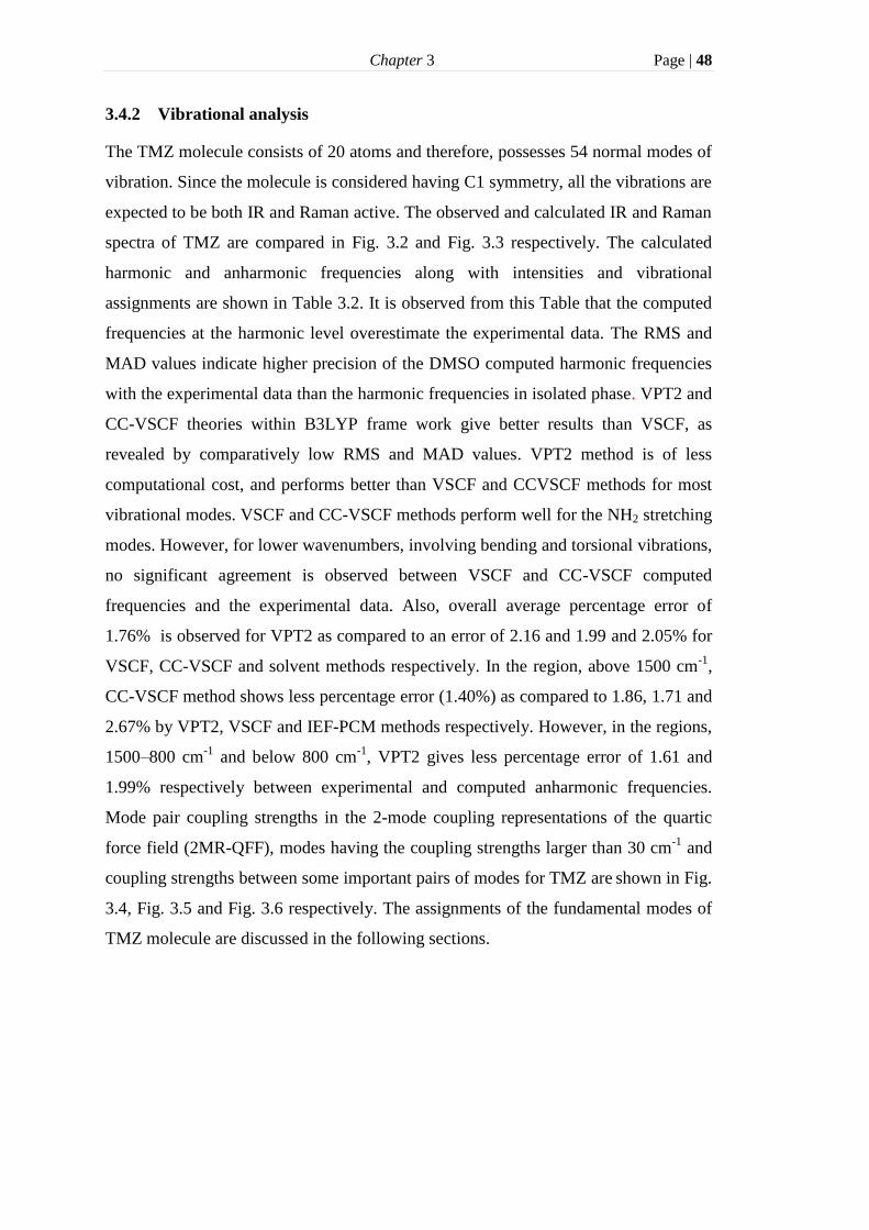
Chapter 3 Page | 48

3.4.2 Vibrational analysis

The TMZ molecule consists of 20 atoms and therefore, possesses 54 normal modes of

vibration. Since the molecule is considered having C1 symmetry, all the vibrations are

expected to be both IR and Raman active. The observed and calculated IR and Raman

spectra of TMZ are compared in Fig. 3.2 and Fig. 3.3 respectively. The calculated

harmonic and anharmonic frequencies along with intensities and vibrational

assignments are shown in Table 3.2. It is observed from this Table that the computed

frequencies at the harmonic level overestimate the experimental data. The RMS and

MAD values indicate higher precision of the DMSO computed harmonic frequencies

with the experimental data than the harmonic frequencies in isolated phase. VPT2 and

CC-VSCF theories within B3LYP frame work give better results than VSCF, as

revealed by comparatively low RMS and MAD values. VPT2 method is of less

computational cost, and performs better than VSCF and CCVSCF methods for most

vibrational modes. VSCF and CC-VSCF methods perform well for the NH2 stretching

modes. However, for lower wavenumbers, involving bending and torsional vibrations,

no significant agreement is observed between VSCF and CC-VSCF computed

frequencies and the experimental data. Also, overall average percentage error of

1.76% is observed for VPT2 as compared to an error of 2.16 and 1.99 and 2.05% for

VSCF, CC-VSCF and solvent methods respectively. In the region, above 1500 cm-1

,

CC-VSCF method shows less percentage error (1.40%) as compared to 1.86, 1.71 and

2.67% by VPT2, VSCF and IEF-PCM methods respectively. However, in the regions,

1500–800 cm-1

and below 800 cm-1

, VPT2 gives less percentage error of 1.61 and

1.99% respectively between experimental and computed anharmonic frequencies.

Mode pair coupling strengths in the 2-mode coupling representations of the quartic

force field (2MR-QFF), modes having the coupling strengths larger than 30 cm-1

and

coupling strengths between some important pairs of modes for TMZ are shown in Fig.

3.4, Fig. 3.5 and Fig. 3.6 respectively. The assignments of the fundamental modes of

TMZ molecule are discussed in the following sections.

Chapter 3 Page | 49

Fig. 3.2 Comparison of the experimental FTIR and theoretical anharmonic spectra of

temozolomide molecule.

Fig. 3.3 Comparison of the experimental FT-Raman and theoretical Raman spectra of

temozolomide molecule.

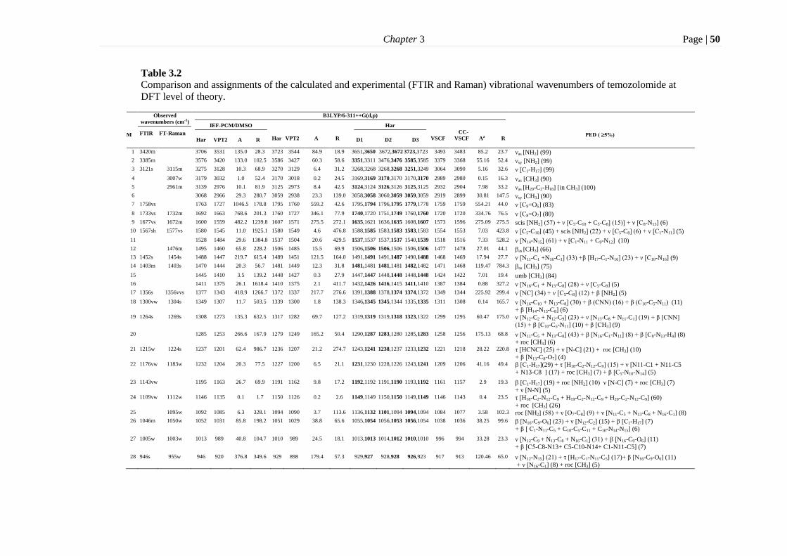
Chapter 3 Page | 50

Table 3.2

Comparison and assignments of the calculated and experimental (FTIR and Raman) vibrational wavenumbers of temozolomide at

DFT level of theory.

M

Observed

wavenumbers (cm-1)

B3LYP/6-311++G(d,p)

PED ( ≥5%)

IEF-PCM/DMSO

Har

VPT2

A

R

Har

VSCF

CC-

VSCF

Aa

R FTIR FT-Raman

Har

VPT2

A

R

D1

D2

D3

1 3420m 3706 3531 135.0 28.3 3723 3544 84.9 18.9 3651,3650 3672,3672 3723,3723 3493 3483 85.2 23.7 νas [NH2] (99)

2 3385m 3576 3420 133.0 102.5 3586 3427 60.3 58.6 3351,3311 3476,3476 3585,3585 3379 3368 55.16 52.4 νsy [NH2] (99)

3 3121s 3115m 3275 3128 10.3 68.9 3270 3129 6.4 31.2 3268,3268 3268,3268 3251,3249 3064 3090 5.16 32.6 ν [C1-H17] (99)

4 3007w 3179 3032 1.0 52.4 3170 3018 0.2 24.5 3169,3169 3170,3170 3170,3170 2989 2980 0.15 16.3 νas [CH3] (90)

5 2961m 3139 2976 10.1 81.9 3125 2973 8.4 42.5 3124,3124 3126,3126 3125,3125 2932 2904 7.98 33.2 νas [H20-C2-H18] [in CH3] (100)

6 3068 2966 29.3 280.7 3059 2938 23.3 139.0 3058,3058 3060,3059 3059,3059 2919 2899 30.81 147.5 νsy [CH3] (90)

7 1758vs 1763 1727 1046.5 178.8 1795 1760 559.2 42.6 1795,1794 1796,1795 1779,1778 1759 1759 554.21 44.0 ν [C9=O6] (83)

8 1733vs 1732m 1692 1663 768.6 201.3 1760 1727 346.1 77.9 1740,1720 1751,1749 1760,1760 1720 1720 334.76 76.5 ν [C8=O7] (80)

9 1677vs 1672m 1600 1559 482.2 1239.8 1607 1571 275.5 272.1 1635,1621 1636,1635 1608,1607 1573 1596 275.09 275.5 scis [NH2] (57) + ν [C5-C10 + C5-C8] (15)] + ν [C8-N13] (6)

10 1567sh 1577vs 1580 1545 11.0 1925.1 1580 1549 4.6 476.8 1588,1585 1583,1583 1583,1583 1554 1553 7.03 423.8 ν [C5-C10] (45) + scis [NH2] (22) + ν [C5-C8] (6) + ν [C1-N11] (5)

11 1528 1484 29.6 1384.8 1537 1504 20.6 429.5 1537,1537 1537,1537 1540,1539 1518 1516 7.33 528.2 ν [N14-N15] (61) + ν [C1-N11 + C9-N12] (10)

12 1476m 1495 1460 65.8 228.2 1506 1485 15.5 69.9 1506,1506 1506,1506 1506,1506 1477 1478 27.01 44.1 βas [CH3] (66)

13 1452s 1454s 1488 1447 219.7 615.4 1489 1451 121.5 164.0 1491,1491 1491,1487 1490,1488 1468 1469 17.94 27.7 ν [N11-C1 +N16-C1] (33) +β [H17-C1-N16] (23) + ν [C10-N16] (9)

14 1403m 1403s 1470 1444 20.3 56.7 1481 1449 12.3 31.8 1481,1481 1481,1481 1482,1482 1471 1468 119.47 784.3 βas [CH3] (75)

15 1445 1410 3.5 139.2 1448 1427 0.3 27.9 1447,1447 1448,1448 1448,1448 1424 1422 7.01 19.4 umb [CH3] (84)

16 1411 1375 26.1 1618.4 1410 1375 2.1 411.7 1432,1426 1416,1415 1411,1410 1387 1384 0.88 327.2 ν [N16-C1 + N13-C8] (28) + ν [C5-C8] (5)

17 1356s 1356vvs 1377 1343 418.9 1266.7 1372 1337 217.7 276.6 1391,1388 1378,1374 1374,1372 1349 1344 225.92 299.4 ν [NC] (34) + ν [C5-C8] (12) + β [NH2] (5)

18 1300vw 1304s 1349 1307 11.7 503.5 1339 1300 1.8 138.3 1346,1345 1345,1344 1335,1335 1311 1308 0.14 165.7 ν [N16-C10 + N13-C8] (30) + β (CNN) (16) + β (C10-C5-N11) (11)

+ β [H14-N13-C8] (6) 19 1264s 1269s 1308 1273 135.3 632.5 1317 1282 69.7 127.2 1319,1319 1319,1318 1323,1322 1299 1295 60.47 175.0 ν [N12-C2 + N12-C9] (23) + ν [N13-C8 + N11-C1] (19) + β [CNN]

(15) + β [C10-C5-N11] (10) + β [CH3] (9)

20 1285 1253 266.6 167.9 1279 1249 165.2 50.4 1290,1287 1283,1280 1285,1283 1258 1256 175.13 68.8 ν [N11-C5 + N13-C8] (43) + β [N16-C1-N11] (8) + β [C8-N13-H4] (8)

+ roc [CH3] (6) 21 1215w 1224s 1237 1201 62.4 986.7 1236 1207 21.2 274.7 1243,1241 1238,1237 1233,1232 1221 1218 28.22 220.8 τ [HCNC] (25) + ν [N-C] (21) + roc [CH3] (10)

+ β [N13-C8-O7] (4) 22 1176vw 1183w 1232 1204 20.3 77.5 1227 1200 6.5 21.1 1231,1230 1228,1226 1243,1241 1209 1206 41.16 49.4 β [C1-H17](29) + τ [H18-C2-N12-C9] (15) + ν [N11-C1 + N11-C5

+ N13-C8 ] (17) + roc [CH3] (7) + β [C5-N10-N14] (5)

23 1143vw 1195 1163 26.7 69.9 1191 1162 9.8 17.2 1192,1192 1191,1190 1193,1192 1161 1157 2.9 19.3 β [C1-H17] (19) + roc [NH2] (10) ν [N-C] (7) + roc [CH3] (7)

+ ν [N-N] (5) 24 1109vw 1112w 1146 1135 0.1 1.7 1150 1126 0.2 2.6 1149,1149 1150,1150 1149,1149 1146 1143 0.4 23.5 τ [H18-C2-N12-C9 + H19-C2-N12-C9 + H20-C2-N12-C9] (60)

+ roc [CH3] (26) 25 1095w 1092 1085 6.3 328.1 1094 1090 3.7 113.6 1136,1132 1101,1094 1094,1094 1084 1077 3.58 102.3 roc [NH2] (58) + ν [O7-C8] (9) + ν [N11-C5 + N13-C8 + N16-C1] (8)

26 1046m 1050w 1052 1031 85.8 198.2 1051 1029 38.8 65.6 1055,1054 1056,1053 1056,1054 1038 1036 38.25 99.6 β [N16-C9-O6] (23) + ν [N12-C2] (15) + β [C1-H17] (7)

+ β [ C1-N11-C5 + C10-C5-C11 + C10-N14-N15] (6)

27 1005w 1003w 1013 989 40.8 104.7 1010 989 24.5 18.1 1013,1013 1014,1012 1010,1010 996 994 33.28 23.3 ν [N12-C9 + N13-C8 + N16-C1] (31) + β [N16-C9-O6] (11)

+ β [C5-C8-N13+ C5-C10-N14+ C1-N11-C5] (7)

28 946s 955w 946 920 376.8 349.6 929 898 179.4 57.3 929,927 928,928 926,923 917 913 120.46 65.0 ν [N12-N15] (21) + τ [H17-C1-N11-C5] (17)+ β [N16-C9-O6] (11)

+ ν [N16-C1] (8) + roc [CH3] (5)

Chapter 3 Page | 51

29 852 837 9.3 152.7 852 836 12.0 25.6 852,852 852,852 852,850 838 836 13.66 34.5 β [Rr] (52) + ν [N12-CH3] (22) + β [CCN] (7) +β [C10-N14-N15] (5)

30 850w 847w 841 803 9.5 15.8 831 842 8.1 2.5 831,831 835,835 875,871 900 893 9.0 67.7 γ [H17-C1] (86)

31 804w 791m 795 806 8.7 78.5 793 814 4.3 20.0 805 815,803 791,791 812 814 3.71 16.1 τ [C1-N11-C5-C10] (71) + γ [C8-C10-N11-C5] (6)

32 736m 744 729 37.3 7.9 742 746 22.0 1.4 743,743 742,739 741,741 743 743 21.42 5.7 γ [O6-N12-N16-C9] [85]

33 704 695 2.6 143.1 699 689 0.7 56.1 700,700 703,702 700,699 701 699 1.16 46.1 ν [Rr] (43)

34 707m 703s 701 703 4.6 41.3 697 709 1.2 14.1 697,694 686,679 695,695 707 705 0.72 28.7 τ [C1-N11-C5-C10] (72) + γ [O6-N12-N16-C9] (6)

+ γ [N14-C5-N16-C10] (7) 35 665 687 100.4 220.6 689 682 55.8 62.7 722,711 697,697 690,690 686 684 60.04 60.4 β [N13-C8-O7] (25) + ν [C8-C5] (15) + roc [NH2] (7)

+ β [N12-N14-N15] (7) 36 636w 665 651 20.7 2.8 665 659 14.6 1.7 652,649 648,630 667,667 695 684 12 0.2 twi [NH2] (64) + τ [H17-C1-N11-C5] (9) + γ [N14-C5-N16-C10] (8)

37 606sh 610s 620 594 10.6 245.7 605 591 5.5 64.7 612,609 604,580 604,604 596 595 5.17 74.6 ν [N12-N15] (42) + β [CNN] (14) + β [N12- C9-O6] (7)

38 583w 587 554 8.3 7.7 590 561 4.9 6.0 552,550 599 591,591 732 726 8.38 11.6 twi [NH2] (66) + τ [C10-N14-N15-N12] (20)

39 562m 578 577 13.8 96.1 574 566 10.8 54.1 589,587 581,580 575,574 572 569 10.48 57.3 β [N13-C8-O7] (47) + ν [N12-N15] (10) + β [C9-N12-N15] (9)

+ roc [NH2] (5) 40 547 547 0.3 1.2 541 557 0.2 0.2 552,550 556,551 542,542 582 576 1.12 5.1 τ [C10-N14-N15-N12] (66) + twi [NH2] (17) + τ [C5-N11-C1-N16] (7)

41 512m 508w 512 501 46.6 25.9 510 503 26.1 22.3 515,512 508,508 511,510 502 501 27.52 31.2 β [CNN] (50) + β [CCN] (6)

42 479vw 472s 469 462 3.9 227.1 468 461 2.0 98.6 477,476 471,463 470,469 464 463 1.79 82.6 β [CCN] (25) + ν [C5-C8] (12) + β [N13-C8-O7] (9)

+ β [C5-C8-N13] (5) 43 331 334 11.2 209.1 331 329 6.3 115.8 357,353 338,338 331,331 348 347 12.78 6.0 β [C5-C8-N13] (28) + ν [C8-C5] (18) + ν [C5-C10] (11)

+ N16-C9-O6 ] (7) +β [CNC] (10) 44 324 298 11.5 160.5 319 323 6.9 50.6 322,320 319,319 322,322 329 327 1.51 153.5 β [N15-N12-CH3] (48) + [N16-C9-O6] (9)

45 360m 316 332 323.0 41.2 301 377 202.3 21.9 526,522 445 296,295 307 304 3.31 38.1 ω [NH2] (82) + τ [N13-C8-C5-C10] (5)

46 333m 303 282 2.4 32.9 300 294 1.0 19.2 308,305 301,301 302,302 571 570 147.01 65.1 β [NCO] (41) + β [C5-C8-N13 + C5-C10-N14] (26)

+ β [C10-N14-N15] (7) 47 280w 269 258 11.2 9.6 251 280 8.4 3.6 259,255 258,254 250,249 313 290 23.42 2.2 γ [C2-C9-N15-N12] (63) + γ [N14-C5-N16-C10] (16)

+ τ [H18-C2-N12-C9 + H19-C2-N12-C9 + H20-C2-N12-C9] (7)

48 261w 242 235 0.5 9.3 236 257 7.1 3.7 255,245 242,240 235,235 343 316 9.99 29.3 τ [Rr] (68) + ω [NH2] (12) + γ [C8-C10-N11-C5] (5)

49 237w 210 221 11.2 147.2 194 242 4.9 31.6 203,200 202,198 190,189 272 246 15.15 174.4 γ [C2-C9-N5-N12] (67) + γ [C8-C10-N11-C5] (6)

50 130s 142 153 13.7 33.8 136 134 8.3 22.2 178,175 151,145 138,137 141 139 8.32 27.8 β [C5-C8- N13] (76) + β [C15-C12-CH3] (6) + β [C5-C10-N14] (5)

51 116 80 3.3 1.6 111 123 4.9 0.0 114,112 118,113 114,110 319 272 0.26 244.8 τ [C1-N11-C5-C10] (56) + γ [C2-C9-N15-N12] (12)

+ γ [N14-C5-N16-N10] (8) 52 105sh 102 80 3.0 103.9 95 174 1.1 52.7 96,93 92,92 104,103 122 122 5.0 118.0 τ [CH3] (72) + τ [N15-N14-C10-N16] (7)

53 81vvs 73 69 0.01 104.4 67 75 0.1 41.0 71 69 69,67 116 95 0.84 164.6 γ [C8-C10-N11-C5] (70) + τ [C1-N11-C5-C10] (11)

+ γ [O6-N12-N16-C9] (5) 54 66s 50 49 13.2 167.5 47 70 3.1 69.1 77 78,76 47,44 98 93 2.29 64.8 twi [O7-C8-NH2] (85)

RMS 78 38 81 36 36 31

MAD 45 26 47 23 25 23

Abbreviation used: M-modes, Har-harmonic wavenumbers, VPT2- anharmonic frequency, A- harmonic IR intensity (km/mol), R- Raman intensity (arb. unit), ν- stretching, sy- symmetric, as- asymmetric, β-

bending, βas - antisymmetric bending, τ- torsional, τ Rr-butterfly motion, scis- scissoring, roc- rocking, ω- wagging, twi- twisting, umb- umbrella motion, γ- out of plane vibrations, w- weak, m- medium

strong, sh- shoulder, s- strong, vs- very strong , vvs- very very strong, Aa-VSCF anharmonic IR intensity (km/mol), bold letter specifies the frequency having high IR intensity than the other one in dimer.

Table 3.2 continued....

Chapter 3 Page | 52

Fig. 3.4 Graphical representation of mode-mode coupling strength in temozolomide.

Fig. 3.5 2D graphical representation of anharmonic mode-mode coupling strength higher than

30 cm-1

in temozolomide molecule.

Chapter 3 Page | 53

Fig. 3.6 Mode-mode coupling strength between important modes of temozolomide.

Carbonyl (C=O) group vibrations

The carbonyl stretching vibrations have been widely studied by infrared

spectroscopy. Since C=O group is highly polar in nature, strong and intense

absorption bands are observed in the region 1700–1750 cm-1

[39,40]. C=O stretching

vibrations are also very important as they take part in hydrogen bonding. The C9=O6

stretching mode (mode 7) is observed at 1758 cm-1

with strong intensity in the FTIR

spectrum of TMZ. The computed anharmonic wavenumbers in the isolated phase are

in agreement with the experimental frequency. The harmonic frequency at 1763 cm-1

in the solvent phase is also comparable with the observed frequency. The assignment

is also in agreement with the literature [41–43]. The carbonyl group, C9=O6, is

involved in hydrogen bonding in D3. The harmonic frequencies for this mode are

1779, 1778 cm-1

in D3. It is clear from Fig. 3.5, that carbonyl vibrations are either not

involved or weakly involved (< 30 cm-1

) in coupling with other modes.

Chapter 3 Page | 54

Amide (CONH2) group vibrations

The title molecule contains only one NH2 group. Therefore, one can expect six

internal modes of vibration as symmetric (νsym) and asymmetric stretching (νasym), the

symmetric planar deformation or scissoring (βs), the anti-symmetric planar

deformation or rocking, the symmetric non-planar deformation or wagging (ω) and

the anti-symmetric non-planar deformation or torsion (τ). In all aromatic amines, NH2

stretching occurs in the 3300–3500 cm-1

region [44]. In solid phase, the asymmetric

and symmetric NH2 stretching vibrations appear at 3350 cm-1

and 3200 cm-1

respectively [44]. In TMZ, the medium intensity bands, observed in the IR spectrum

at 3420 cm-1

(mode 1) and 3385 cm-1

(mode 2), are assigned to NH2 asymmetric and

symmetric stretching vibrations respectively. Large deviations between the observed

and calculated (VPT2) NH2 stretching frequencies are observed, both in the isolated

and solvent phases. The deviations are due to strong coupling of NH2 stretching

modes (1 and 2) with mode 46 [Fig. 3.6]. The deviations may also be due to the

intermolecular hydrogen bonding, N‒H···O or N‒H···N, in D1 and D2 respectively.

In dimer D1, the calculated frequencies for mode 1(3651,3650 cm-1

) and mode 2

(3351,3311 cm-1

) show better agreement to respective observed frequencies than

those are in D2 and D3. The NH2 stretching modes show significant anharmonic

corrections in VSCF and CC-VSCF levels of theory. The calculated frequencies of

asymmetric and symmetric stretching modes of NH2 are respectively 3483 and 3368

cm-1

at CC-VSCF and 3493 and 3379 cm-1

at VSCF level of theory.

The NH2 scissoring vibrations are usually observed in the region 1650‒1620

cm-1

[45]. According to PED calculations, the NH2 scissoring mode is mixed with

C‒C and C‒N stretching vibrations and contributes to mode 9 (57% PED) and 10

(22% PED). The vibrational frequencies observed at 1677 cm-1

and 1672 cm-1

in IR

and Raman spectrum, respectively, are assigned to mode 9. Mode 10 has been

observed at 1567 cm-1

in IR spectrum and at 1577 cm-1

in Raman spectrum. The

computed anharmonic frequencies for mode 9 are deviated from the observed

frequencies. The deviation may be associated to the high anharmonicity of this mode

[46]. Also, significant coupling strengths (>30 cm-1

) are observed between mode pairs

9 and 1 as well as 9 and 2 [Fig. 3.5]. The deviations between the computed and

observed wavenumbers for mode 9 are lower in D1 and D2 dimers. The NH2 rocking

vibrations are observed in the region 1125 ± 45 cm-1

[47,48]. In the present study, this

Chapter 3 Page | 55

vibration is observed in mode 25 at 1095 cm-1

in the Raman spectrum. The

anharmonic frequency, 1090 cm-1

, calculated using VPT2 theory in the isolated phase

and the harmonic frequency at 1092 cm-1

in the solvent, are in close agreement with

observed one. The non-planar modes (36 and 38) of the NH2 group have, respectively,

64% and 66% PED contribution from NH2 twisting vibrations. These modes are

observed at 636 cm-1

in IR spectrum and at 583 cm-1

in Raman spectrum respectively.

Mode 38 is strongly coupled to modes 46 and 48. The large deviations of the

experimental and simulated anharmonic frequencies, corresponding to modes 36 and

38, may be due to the improper definition of potential energy surface or limitations in

the Cartesian coordinate system [49]. The harmonic vibrational frequencies in

monomer and D3, corresponding to mode 38, are in agreement with the observed

frequency. The twisting vibration of NH2 group about C8–O7 bond (mode 54) is

observed at 66 cm-1

in Raman spectrum. The NH2 wagging vibration, observed at 360

cm-1

, is assigned to mode 45.

The band due to the C=O stretching vibrations is often referred as the amide I

band. It is generally observed in the region 1670–1650 cm-1

having strong intensity

[45]. In the present study, C8=O7 stretching vibration (mode 8) is observed at 1733

cm-1

in IR spectrum and at 1732 cm-1

in the Raman spectrum. The corresponding

anharmonic frequency, 1727 cm-1

, predicted at VPT2 theory in isolated phase, is in

agreement with the experimental frequency. Significant coupling between modes 8

and 54 has also been predicted [Fig. 3.5].

Methyl (CH3) group vibrations

Methyl groups are generally referred as an electron donating substitution in

the aromatic ring system. Since the title molecule contains only one CH3 group

attached to the aromatic ring, nine fundamentals are expected. The C‒H stretching

vibrations in CH3 group normally appear in the region 3010‒2880 cm-1

[50–52]. In

the present study, the anharmonic C‒H stretching frequencies of CH3 group,

computed at VPT2 theory, have better agreement with the experimental

wavenumbers. However, the wavenumbers computed in gas phase are more close to

the experimental data than the wavenumbers computed in solvent phase. The C‒H

asymmetric stretching vibration in the methyl group is assigned to mode 4. The

computed VPT2 frequency in isolated phase at 3018 cm-1

, is ascribed to this mode.

Chapter 3 Page | 56

The symmetric C–H stretching vibration, computed at 2938 cm-1

, is assigned to mode

6. These vibrations are pure stretching vibrations as evident by PED values. The

assignment of the CH3 stretching frequencies clearly signifies that these frequencies

do not significantly depend on the surroundings of the functional group.

The CH3 asymmetric bending modes, 12 and 14, are observed at 1476 cm-1

and at 1403 cm-1

in the Raman spectrum. The CH3 symmetric bending frequency

(umbrella motion) is not observed in IR and Raman spectra. The anharmonic

frequencies, calculated at 1422 cm-1

(CC-VSCF), 1424 cm-1

(VSCF) and 1427 cm-1

(VPT2/isolated), correspond to the umbrella motion of methyl group. The CC-VSCF

anharmonic frequencies, 1478 cm-1

and 1468 cm-1

, are assigned to CH3 asymmetric

bending vibrations. These assignments are within the region as reported in the

literature [53–56]. The CH3 torsional mode generally appears in the low frequency

region and is assigned to mode 52 with 72% PED contribution. The Raman frequency

for this mode is observed at 105 cm-1

. The harmonic wavenumbers, 104 and 103 cm-1

in D3, are in agreement with the observed wavenumbers.

C-X vibrations

The C–H stretching vibrational bands normally appear in the region 3080–

3010 cm-1

[44,51]. The intense band, observed at 3121 cm-1

in the IR spectrum and at

3115 cm-1

in Raman spectrum, shows the presence of C1–H17 stretching frequency. It

is animated as pure stretching and is assigned to mode 3. The frequencies, 3129 cm-1

in isolated phase and 3128 cm-1

in solvent phase, computed at VPT2 level of theory,

is in agreement with the observed frequency. As evident from Fig.3.6, strong coupling

is observed between modes 3 and 30. Mode 3 is also significantly coupled to mode 22

and 14. The C1‒H17 in-plane bending vibrations, mixed with other vibrations, have

contributions in mode 22, 23 and 26. The IR bands observed at 1176, 1143 and 1046

cm-1

are assigned to these bending modes. These assignments are well within the

reported regions [56,57].

Ring vibrations

The ring stretching vibrations are complicate combinations of mainly C‒C,

C‒N and N‒N vibrations. The assignment of these vibrations is a difficult task, since

the mixing of the vibrations occurs. In our work, mode 10 is assigned to C‒C

Chapter 3 Page | 57

stretching vibration mixed with NH2 scissoring and C‒N stretching vibrations. The

most important ring stretching vibration is the ring breathing in which all bonds of the

ring stretch and contract in-phase. It is predicted at 699 cm-1

in mode 33 using CC-

VSCF method. The computed frequencies for the breathing mode is in close

agreement with the literature [58,59]. Another important vibration is the butterfly

motion in TMZ. This vibration presents a mixed profile and assigned to mode 48. The

frequency of this mode is observed at 261 cm-1

in Raman spectrum and well predicted

at 257cm1 by VPT2 level of theory in the isolated phase.

3.4.3 UV-Vis and HOMO–LUMO analysis

TD-DFT method has become one of the most popular and widely used approaches for

the calculation of properties, such as excitation energies, oscillator strengths and

excited state geometries of medium to large molecular systems [60]. TD-DFT has

been widely used to find out the low lying excited states of molecules on the basis of

fully optimized ground-state structure [61]. The vertical excitation energies,

absorption wavelengths and oscillator strengths (f) of TMZ molecule along with their

assignments are given in Table 3.3 and the experimental and simulated electronic

spectra of TMZ are shown in Fig. 3.7.

Table 3.3

Theoretical and experimental UV spectral characteristics of temozolomide molecule.

Experimental B3LYP/6-311++G(d,p)

λobs(nm) E

(eV)

λcal(nm) (f) E

(eV)

Composition (˃5%)

320 0.001 3.87 H-1→LUMO (89%), H-3→LUMO (9%)

317 3.87 315 0.334 3.94 HOMO→LUMO (94%) 296 0.004 4.19 H-3→LUMO (89%), H-1→LUMO (8%)

275 0.0246 4.50 H-2→LUMO (99%)

245 5.01 252 0.1077 4.93 HOMO→L+1 (83%), H-4→LUMO (7%) 243 0.0007 5.11 H-5→LUMO (98%)

233 0.0001 5.32 H-3→L+1 (23%), H-1→L+1 (66%),

H-7→LUMO (8%)

231 0.0001 5.38 H-7→LUMO (73%), H-1→L+1 (15%)

230 0.0125 5.38 H-6→LUMO (13%), H-4→LUMO (76%) 223 0.0005 5.56 H-7→LUMO (12%), H-3→L+1 (68%),

H-1→L+1 (14%)

217 0.0026 5.72 H-2→L+1 (89%), HOMO→L+2 (7%) 216 0.000 5.75 H-1→L+2 (86%)

214 0.0896 5.80 H-6→LUMO (37%), H-4→LUMO (13%),

HOMO→L+2 (33%), H-2→L+1 (9%), 206 5.96 207 0.2545 5.98 H-6→LUMO (41%), HOMO→L+2 (50%)

202 0.003 6.13 H-5→L+1 (84%), H-7→L+1 (9%)

Abbreviation used: λ- Excitation wavelength, E-Excitation energy, H-Homo, L-Lumo, f-

Oscillator strength

Chapter 3 Page | 58

Fig. 3.7 Experimental and simulated UV-Vis spectra of temozolomide molecule.

Fig. 3.8 Frontier molecular orbitals of temozolomide molecule in isolated phase.

Chapter 3 Page | 59

Fig. 3.9 Density of state (DOS) spectrum of temozolomide molecule.

The TD-DFT calculations in ethanol solution show three intense bands at 315, 252

and 207 nm having the oscillator strengths as 0.334, 0.1077 and 0.2545 respectively.

These absorptions are found to be in good agreement with the experiment values. The

maximum absorption wavelength observed at 317 nm corresponds to

HOMO→LUMO (94%) electronic transition. The absorption wavelengths, 245 and

206 nm, are assigned to HOMO→LUMO+1 (83%) and HOMO→LUMO+2 (50%)

transitions respectively. The assignments of other transitions are also shown in Table

3.3.

The pictorial representation of HOMO‒LUMO orbitals and energy gap of

TMZ are shown in Fig. 3.8 and the density of state spectrum of is shown in Fig. 3.9.

The HOMO–LUMO energy gap characterizes the chemical activity, optical

polarizibility and chemical hardness‒softness of the molecule [62]. The frontier

molecular orbital energy gap is found to be 4.45 eV. The energy gap of (HOMO‒1)–

(LUMO+1) is 5.69 eV. A large HOMO–LUMO energy gap is an indication of high

stability of TMZ. It can be seen from the HOMO–LUMO plots that HOMO is spread

over the entire molecule except the NH2 group. The LUMO is also spread over the

entire molecule except CH3 group.

3.4.4 Natural charge and electron population analysis

Natural charge and electron population analysis describe the distribution of electrons

in core, valence and Rydberg atomic orbitals. Natural population analysis is an

Chapter 3 Page | 60

alternative to conventional Mulliken population analysis having improved numerical

stability and clearly describes the electron distribution in compounds [63]. The natural

and Mulliken charges of the monomer and dimer structures of the title molecule are

presented in Table 3.4. The comparison between the computed charges are plotted in

Fig. 3.10. Among all the carbon atoms, only C2 atom has got the negative charge. All

the nitrogen and oxygen atoms, except N15, exhibit negative charge. The

electronegative atoms have the tendency to attract the electron cloud towards itself. In

TMZ molecule, the large natural positive and negative charges are calculated for C9

and N13 atoms respectively.

Table 3.4

Natural and Mulliken atomic charges of temozolomide at B3LYP/6-311++G(d,p) level of

theory.

Atom Natural charges Mulliken charges

Monomer D1 D2 D3 Monomer D1 D2 D3

C1 0.248 0.253 0.263 0.255 0.362 0.410 0.269 -0.332

C2 -0.354 -0.354 -0.355 -0.357 -0.240 -0.243 -0.217 -0.226

H3 0.404 0.395 0.386 0.409 0.282 0.294 0.535 0.279

H4 0.394 0.424 0.379 0.397 0.330 0.570 0.304 0.351

C5 0.046 0.056 0.090 0.066 0.341 -0.355 0.091 0.097

O6 -0.573 -0.579 -0.576 -0.639 -0.266 -0.265 -0.250 -0.389

O7 -0.594 -0.649 -0.608 -0.600 -0.346 -0.329 -0.328 -0.339

C8 0.631 0.670 0.631 0.629 0.048 0.348 -0.314 0.580

C9 0.812 0.820 0.820 0.885 0.280 0.255 0.269 0.290

C10 0.277 0.282 0.285 0.267 -0.774 -0.425 -0.254 -0.721

N11 -0.465 -0.461 -0.510 -0.483 -0.109 -0.055 -0.099 -0.086

N12 -0.302 -0.312 -0.311 -0.305 -0.124 -0.147 -0.035 0.038

N13 -0.789 -0.756 -0.813 -0.795 -0.397 -0.632 -0.581 -0.433

N14 -0.167 -0.177 -0.167 -0.151 -0.537 -0.507 -0.371 -0.437

N15 0.015 0.009 0.014 -0.007 0.546 0.509 0.369 0.396

N16 -0.448 -0.453 -0.446 -0.453 -0.213 -0.237 -0.205 -0.323

H17 0.217 0.220 0.231 0.250 0.240 0.254 0.265 0.762

H18 0.210 0.212 0.212 0.211 0.196 0.197 0.198 0.196

H19 0.226 0.226 0.227 0.231 0.188 0.190 0.194 0.200

H20 0.211 0.212 0.212 0.212 0.196 0.197 0.198 0.196

Fig. 3.10 Comparison of the natural and mulliken charges of temozolomide molecule.

Chapter 3 Page | 61

3.4.5 Natural bond orbital analysis

NBO analysis is an important technique for studying intra and inter molecular

interactions. It provides a convenient basis for investigating charge transfer or

conjugative interaction in molecular systems [64]. The NBO calculations perform

energetic analysis of NBO interactions based on the one electron effective energy

operator i.e. Fock matrix. All the possible interactions between filled NBOs

(donor) and empty NBOs (acceptor) with their interaction energy are estimated by

second order perturbation theory. The two electron stabilization energy E(2)

associated

with delocalization, i→j, for each donor NBO (i) and acceptor NBO (j) is computed

by second order perturbation theory using equation

where, is the occupancy of donor orbital; and are

diagonal elements and are the off diagonal elements of NBO

Fock matrix. This equation describes the donor-acceptor interactions in the NBO

analysis [64].

The NBO analysis of TMZ is carried out at the DFT/B3LYP level of theory

using NBO 3.1 program [38] implemented in the Gaussian 09 package [25]. The

hybridization of filled orbitals, bond type, occupancy and electron densities of atoms

involved in natural bonding is shown in Table 3.5. The NBO analysis has predicted

high occupancies for σ(O6‒C9), σ(O7‒C8) and σ(C8‒N13) bonding. The occupancies

of the orbitals below 2.0 indicate the deviations from ideal Lewis structure [65]. In

order to understand these small deviations from idealized Lewis structure, the donor-

acceptor interactions are adopted. The second order perturbation energy values, E(2)

[66], corresponding to the interactions and the overlap integral of orbital pairs are

presented in Table 3.6. The strongest hyperconjugative interaction with E(2)

= 61.34

kcal/mol is observed between the orbitals containing lone pair of electrons of N13 of

the NH2 group with the neighboring π*(O7‒C8)

antibonding orbital. The lone pair of

electrons of N16 shows strong hyperconjugation with the antibonding orbitals of

π*(C1‒N11), π

*(C5‒C10) and π

*(O6‒C9) with E

(2) values; 40.06, 31.60 and 49.12

kcal/mol respectively. Other interactions between NBO's having large E(2)

are

n(LP2O6)→σ*(C9‒N12), n(LP2O6)→σ*(C9‒N16), n(LP2O7)→σ*(C5‒C8),

Chapter 3 Page | 62

n(LP2O7)→σ*(C8‒N13), n(LP1N12)→σ*(C2‒H18) and (LP1N12)→π*(N14‒N15).

The existence of three dimers of TMZ has also been verified by NBO analysis. The

stabilization energies, E(2)

, which determine the strength of hydrogen bonding in three

TMZ dimer structures are also tabulated in Table 3.6. The intermolecular hydrogen

bonds are formed by overlapping between the n(LPO) and σ*(N‒H) orbitals in D1,

n(LPO) and σ*(C‒H) orbitals in D3 as well as n(LPN) and σ*(N‒H) orbitals in D2.

The intermolecular hydrogen bonding interactions in D2 and D3 have high

stabilisation energies.

Table 3.5

NBO analysis of temozolomide at B3LYP/6-311++G(d,p) level of theory.

Bond (A-B) Occupancy EDA% EDB% NBO (% p character)

σ (C1‒N11) 1.98502 41.28 58.72 0.6425sp1.83(64.64)C+ 0.7663sp1.74(63.37)N

π C1‒N11) 1.85226 42.15 57.85 0.6492sp1.00(99.79)C+ 0.7606sp0.00(99.82)N

σ (C1‒N16) 1.98527 34.94 65.06 0.5911sp2.43(70.73)C+ 0.8066sp1.91(65.63)N

σ (C1‒H17) 1.98475 61.28 38.72 0.7828sp1.80 (64.21)C+ 0.6222sp0.00(0.06)H

σ (C2‒N12) 1.98633 35.20 64.80 0.5933sp3.42(77.25)C+ 0.8050sp1.93(65.82)N

σ (C2‒H8) 1.98722 60.63 39.37 0.7787sp2.86 (74.06)C+ 0.6274sp0.00(0.04)H

σ (C2‒H19) 1.98851 61.32 38.68 0.7831sp2.88 (74.20)C+ 0.6219sp0.00(0.04)H

σ (C2‒H20) 1.98722 60.63 39.37 0.7787sp2.86 (74.06)C+ 0.6274sp0.00(0.04)H

σ (H3‒N13) 1.98983 29.48 70.52 0.5429sp0.00(0.06)H+ 0.8398sp2.19(68.63)N

σ (H4‒N13) 1.98993 30.02 69.98 0.5479sp0.00(0.05)H+ 0.8365sp2.34(70.05)N

σ (C5‒C8) 1.97588 52.83 47.17 0.7269sp1.86 (65.06)C+ 0.6868sp0.00(65.89)C

σ (C5‒C10) 1.97717 48.84 51.16 0.6989sp1.74 (63.45)C+ 0.7153sp1.43(58.74)C

π (C5‒C10) 1.74727 49.62 50.38 0.7044sp1.00 (99.95)C+ 0.70981.00(99.98)C

σ (C5‒N11) 1.97365 41.54 58.46 0.6445sp2.50(71.34)C+ 0.7646sp2.15 (68.16)N

σ (O6‒C9) 1.99081 63.66 36.34 0.7979sp1.40 (58.24)O+ 0.6029sp1.76 (63.73)C

π (O6‒C9) 1.98869 69.71 30.29 0.8349sp1.00(99.87)O+ 0.5503sp1.00 (99.51)C

σ (O7‒C8) 1.99325 63.95 36.05 0.7997sp1.37 (57.79)O+ 0.6004sp1.97 (66.19)C

π (O7‒C8) 1.98174 69.65 30.35 0.8346sp1.00(99.87)O+ 0.5509sp1.00 (99.53)C

σ (C8‒N13) 1.99377 39.12 60.88 0.6254sp2.12(67.87)C+ 0.7803sp1.60(61.48)N

σ (C9‒N12) 1.98634 37.62 62.38 0.6133sp2.06(67.26)C+ 0.7898sp1.80(64.27)N

σ (C9‒N16) 1.98465 36.12 63.88 0.6010sp2.20(68.81)C+ 0.7992sp1.96(66.24)N

σ (C10‒N14) 1.98460 43.01 56.99 0.6558sp2.07(67.36)C+ 0.7549sp2.00(66.60)N

σ (C10‒N16) 1.97959 36.26 63.74 0.6022sp2.83(73.79)C+ 0.7984sp2.14(68.08)N

σ (N12‒N15) 1.98959 55.05 44.95 0.7419sp2.32(69.82)N+ 0.6705sp3.11(75.58)N

σ (N14‒N15) 1.98870 49.59 50.41 0.7042sp2.03(69.82)N+ 0.7100sp1.78(64.00)N

π (N14‒N15) 1.91925 51.05 48.95 0.7145sp1.00(99.70)N+ 0.6996sp1.00(99.71)N

LP1O6 Sp0.71(41.53)

LP2O6 Sp1.00(99.91)

LP1O7 Sp0.72 (42.00)

LP2O7 sp99.99(99.87)

LP1N11 Sp2.14(68.09)

LP1N12 Sp1.00(99.99)

LP1N13 sp99.99(99.74)

LP1N14 Sp1.95(66.08)

LP1N15 Sp1.49(59.86)

LP1N16 Sp1.00(100)

Abbreviation used: ED-Electron density

Chapter 3 Page | 63

Table 3.6

Second order perturbation analysis of Fock matrix of temozolomide at B3LYP/6-

311++G(d,p) level of theory.

Donor-acceptor interaction E(2)a

(kcal/mol)

E(j)-E(i)b

(a.u)

F(i,j)c

(a.u)

n(LP1O6)→σ*(C9‒N12) 1.58 1.12 0.038

n(LP1O6)→σ*(C9‒N16) 1.50 1.10 0.037

n(LP2O6)→σ*(C9‒N12) 28.08 0.69 0.127

n(LP2O6)→σ*(C9‒N16) 29.71 0.67 0.128

n(LP1O7)→σ*(C5‒C8) 1.80 1.08 0.040

n(LP1O7)→σ*(C8‒N13) 1.58 1.15 0.039

n(LP2O7)→σ*(C5‒C8) 22.11 0.66 0.109

n(LP2O7)→σ*(C5‒N11) 0.63 0.70 0.019

n(LP2O7)→σ*(C8‒N13) 26.53 0.720 0.126

n(LP1N11)→σ*(C1‒N16) 7.59 0.81 0.071

n(LP1N11)→σ*(C1‒H17) 2.31 0.79 0.039

n(LP1N11)→σ*(H3‒N13) 0.78 0.85 0.023

n(LP1N11)→σ*(C5‒C8) 1.84 0.81 0.035

n(LP1N11)→σ*(C5‒C10) 5.22 0.98 0.065

n(LP1N11)→σ*(C9‒N16) 0.81 0.77 0.022

n(LP1N11)→σ*(C10‒N14) 0.54 0.82 0.019

n(LP1N12)→σ*(C2‒H18) 40.15 0.69 0.053

n(LP1N12)→σ*(C2‒H20) 4.14 0.69 0.053

n(LP1N12)→π*(N14‒N15) 42.73 0.26 0.098

n(LP1N13)→π*(O7‒C8) 61.34 0.30 0.121

n(LP1N14)→σ*(C5‒C10) 0.56 0.97 0.021

n(LP1N14)→σ*(C10‒N16) 10.51 0.80 0.083

n(LP1N14)→σ*(N12‒N15) 18.47 0.72 0.104

n(LP1N15)→σ*(C9‒N12) 10.36 0.84 0.084

n(LP1N15)→σ*(C10‒N14) 11.53 0.86 0.089

n(LP1N16)→π*(C1‒N11) 40.06 0.30 0.101

n(LP1N16)→π*(C5‒C10) 31.60 0.32 0.092

n(LP1N16)→π*(O6‒C9) 49.12 0.29 0.111

Dimer

From Unit 1 to 2 (dimer D1)

n(LP1O7)→σ*(N33‒H24) 4.97 1.11 0.066

n(LP2O7)→σ*( N33‒H24) 9.96 0.69 0.076

From Unit 2 to 1 (dimer D1)

n(LP1O27)→σ*(N13‒H4) 4.90 1.13 0.067

n(LP2O27)→σ*( N13‒H4) 9.58 0.71 0.075

From Unit 1 to 2 (dimer D2)

n(LP1N11)→σ*( N33‒H23) 36.28 0.91 0.165

From Unit 2 to 1 (dimer D2)

n(LP1N31)→ σ*(N13‒H3) 75.52 0.96 0.243

From Unit 1 to 2 (dimer D3)

n(LP1O6)→ σ*(C21‒H37) 41.95 1.10 0.192

n(LP2O6)→ σ*(C21‒H37) 96.54 1.13 0.297

From Unit 2 to 1 (dimer D3)

n(LP1O26)→ σ*(C1‒H17) 58.09 1.17 0.233

n(LP2O26)→ σ*(C1‒H17) 46.66 0.98 0.193 aStabilisation (delocalization) energy. bEnergy difference between i (donor) and j (acceptor) NBO orbitals. cFock matrix element i and j NBO orbitals.

3.4.6 Molecular electrostatic potential

Molecular electrostatic potential (MEP) is used to predict the reactive behaviour of

molecules in both electrophilic and nucleophilic reactions, study of biological

recognition processes and hydrogen bonding interactions. MEP mapping is very

useful in the investigation of molecular structure with its physiochemical property

relationships [67–70]. The MEP plotted on the isodensity surface of the molecule is

related to the electronegativity and the partial charges on the different atoms of the

Chapter 3 Page | 64

molecule [71]. Red and blue areas in MEP refer to the regions of negative and

positive potentials, corresponding to the electron rich and electron poor regions

respectively. The green color signifies the neutral electrostatic potential. The MEP of

TMZ, simulated using B3LYP/6-311++G(d,p) level of theory, with color range from

‒7.243e-2 (deepest red) to 7.243e-2 (deepest blue) is shown in Fig. 3.11. The MEP

shows that O7 atom (‒0.714 a.u.) represents the most negative potential region and is

vulnerable to an electrophilic attack. Hydrogen atoms of methyl group have high

positive potential. The knowledge of the molecular reactive site enables workers to

predict how complex drugs interact with proteins.

Fig. 3.11 Molecular electrostatic potential map of temozolomide molecule.

3.4.7 Thermodynamic and NLO properties

The theoretical data obtained during geometry optimization provides various

molecular properties. Thermodynamic data are important for understanding many

chemical processes. The quantum chemical calculations also play a critical role in

designing non-linear optical (NLO) molecules and predicting some related properties

such as molecular dipole moments, polarizabilities and hyperpolarizabilities [72]. The

computation of polarizabilities and hyperpolarizabilities of the organic compounds are

of great significance to study the phenomenon induced by intermolecular interactions

and non-linear optical effect. The energies, thermodynamic parameters and nonlinear

Chapter 3 Page | 65

optical properties (NLO) of TMZ have been calculated at DFT level of theory using

6-311++G(d,p) basis set. The calculated SCF energy, zero-point vibrational energy,

thermal energy, enthalpy, entropy, dipole moment and molar capacity at constant

volume and pressure (Cp and Cv) are listed in Table 3.7. The NLO parameters are

given in Table 3.8. The mean first order hyperpolarizability was obtained using

the following equation:

The computed value of is 2.93×10-30

esu, which is 7.86 times more than that of

urea (0.3728×10-30

esu). The high value of first order hyperpolarizability reflects non-

linear property of the molecule.

Table 3.7

Zero point vibrational energy (kcal mol-1

), thermal energy (kcal mol-1

), entropy(cal mol-1

K-1

),

enthalpy (kcal mol-1

), molar heat capacity at constant volume and pressure (cal mol-1

K-1

) and

dipole moment (Debye) of temozolomide molecule.

Parameters B3LYP/6-311++G(d,p)

Harmonic Anharmonic

Zero-point vibrational energy 87.71 87.028

Energy 95.25 94.321

Enthalpy 95.843 94.910

Entropy 109.16 105.93

Molar heat capacity at constant volume (Cv) 44.015 44.015

Molar heat capacity at constant pressure (Cp) 46.003 46.007

Dipole moment 3.4974

Table 3.8

Calculated components of polarizability (a.u.), first order hyperpolarizability β (a.u.), mean

polarizability ‹α› (a.u.), anisotropy of the polarizability γ (a.u.) and the mean first order

hyperpolarizability β0 (esu, 1 a.u.=8.639 x 10–33

esu) of temozolomide.

αxx 184.96 βxxx 326.86

αxy 8.42 βxxy -338.14

αyy 128.45 βxyy -97.18

αxz 0.000 βyyy 64.04

αyz 0.000 βxxz –0.01

αzz 64.87 βxyz 0.000

‹ α › 126.09 βyyz 0.00

γ 105.08 βxzz 14.52

βyzz 39.20

βzzz 0.01

β0 (esu) 2.93 x 10–30

Chapter 3 Page | 66

3.5 Conclusions

The geometrical parameters of the monomer and dimer structures of temozolomide

have been calculated using DFT method with 6-311++G(d,p) basis set. The hydrogen

bonding interactions between two monomeric units of the title molecule are also

studied. The assignments of FTIR and FT-Raman spectra are supported by the

anharmonic calculations using VPT2 method, VSCF and CC-VSCF approaches

within the DFT framework. VPT2 and CC-VSCF theories within B3LYP framework

give better results than VSCF, as revealed by comparatively low RMS and MAD

values. However, VPT2 has lesser computational cost, at least an order of magnitude

cheaper than VSCF and CC-VSCF. Although, the harmonic frequencies computed

using IEF-PCM model have a better agreement than the DFT/6-311++G(d,p)

computed harmonic frequencies, but the anharmonic frequencies have larger RMS

and MAD values. In general, a good agreement between the experimental and

calculated frequencies has been achieved. The possible formation of dimers is

confirmed by NBO analysis. The deviations of the NH2 stretching modes from the

experiment are observed due to the high anharmonicity associated with these modes

or the neglect of higher order terms in potential expression. These modes are

corrected well by VSCF and CC-VSCF approaches than VPT2 algorithm. UV‒Vis

experimental and calculated data are in agreement with each other. The HOMO and

LUMO energy eigenvalues support the charge transfer within the molecule. The MEP

analysis shows that O7 atom is vulnerable to an electrophilic attack and represents the

most negative potential region.

Chapter 3 Page | 67

References

[1]. D. Zhang, A. Tian, X. Xue, M. Wang, B. Qiu, A. Wu, Int. J. Mol. Sci. 13

(2012) 1109‒1125.

[2]. H.S. Friedman, T. Kerby, H. Calvert, Clin. Cancer Res. 6 (2000) 2585‒2597.

[3]. W.P. Mason, J.G. Cairncross, Nat. Clin. Pract. Neurol. 1 (2005) 88–95.

[4]. E.S. Newlands, M.F. Stevens, S.R. Wedge, R.T. Wheelhouse, C. Brock,

Cancer Treat. Rev. 23 (1997) 35–61

[5]. M.J.M. Darkes, G.L. Plosker, B. Jarvis, Am. J. Cancer 1 (2002) 55–80.

[6]. L.Tentori, G. Graziani, Curr. Med. Chem. 16 (2009) 245‒257.

[7]. M.J.M. Darkes, G.L. Plosker, B. Jarvis, Am. J. Cancer 1 (2002) 55‒80.

[8]. P. Suppasansatorn, G. Wang, B.R. Conway, W. Wang, Y. Wang, Cancer Lett.

244 (2006) 42–52.

[9]. T. Lopez, J. Sotelo, J. Navarrete, J.A. Ascencio, Opt. Mater. 29 (2006) 88‒94.

[10]. A.A Razak, S. K. Masthanamma, B. Omshanthi, V. Suresh, P. Obulamma, Int.

J. Pharm. Sci. Res. 4 (2013) 1419‒1423.

[11]. H. Kim, P. Likhari, D. Parker, P. Statkevich, A. Marco, C.C. Lin, A.A.

Nomeir, J. Pharm. Biomed. Anal. 24 (2001) 461‒468.

[12]. N.J. Babu, P. Sanphui, A. Nangia, Chem. Asian J. 7 (2012) 2274 –2285.

[13]. Xin-Hua Tian, Xiao-Ning Lin, F. Wei, W. Feng, Zhi-Chun Huang, P.B. Wang,

L. Ren, Y. Diao, Int. J. Nanomedicine 6 (2011) 445‒452.

[14]. M. Laszcz, M. Kubiszewski, L. Jedynak, M. Kaczmarska, L. Kaczmarek, W.

Luniewski, K. Gabarski, A. Witkowska, K. Kuziak, M. Malinska, Molecules

18 (2013) 15344‒15356.

[15]. O.E. Kasende, A. Matondo, M. Muzomwe, J.T. Muya, S. Scheiner, Comp.

Theor. Chem. 1034 (2014) 26‒31.

[16]. M. Castella-Vantura, E. Kassab, G. Buntinx, O. Poziat, Phys. Chem. Chem.

Phys. 2 (2000) 4682‒4689.

[17]. D.N. Shin, J.W. Hahn, K.H. Jung, T.K. Ha, J. Raman Spectrosc. 29 (1988)

245‒249.

[18]. J. Neugebauer, M. Reiher, C. Kind, B.A. Hess, J. Comput. Chem. 23 (2002)

895‒910.

[19]. C.Y. Lin, A.T.B. Gilbert, P.M.W. Gill, Theor. Chem. Acc. 120 (2008) 23‒35.

Chapter 3 Page | 68

[20]. C. James, A.A. Raj, R. Reghunathan, V.S. Jayakumar, I.H. Joe, J. Raman

Spectrosc. 37 (2006) 1381‒1392.

[21]. M.A. Broda, A. Buczek, T. Kupka, J. Kaminsky, Vib. Spectros. 63 (2012)

432‒439.

[22]. V. Barone, J. Chem. Phys. 122 (2005) 14108‒14118.

[23]. G. M. Chaban, J. O. Jung, R. B. Gerber, J. Chem. Phys. 111 (1999)

1823‒1829.

[24]. C. Minichino, V. Barone, J. Chem. Phys. 100 (1994) 3717‒3741.

[25]. M.J. Frisch, G.W. Trucks, H.B. Schlegel, G.E. Scuseria, M.A. Robb, J.R.

Cheeseman, et. al., Gaussian 09, Revision D.01, Gaussian, Inc., Wallingford

CT, 2009.

[26]. A. D. Becke, Phys. Rev. A 38 (1988) 3098‒3100.

[27]. A. D. Becke, J. Chem. Phys. 98 (1993) 5648‒5652.

[28]. B.G. Johnson, M.J. Frisch, Chem. Phys. Lett. 216 (1993) 133‒140.

[29]. C. Lee, W. Yang, R. G. Parr, Phys. Rev. B 37 (1988) 785‒89.

[30]. G. Keresztury, S. Holly, G. Besenyei, J. Varga, A. Wang, J.R. Durig,

Spectrochim. Acta A 49 (1993) 2007–2026.

[31]. M.W. Schmidt, K.K. Baldridge, J.A. Boatz, S.T. Elbert, M.S. Gordon, et. al.,

J. Comput. Chem. 14 (1993) 1347–1363.

[32]. C. Capelli, S. Monti, G. Scalmani, V. Barone, J. Chem. Theory Comput. 6

(2010) 1660–1669.

[33]. R. Cammi, J. Tomasi, J. Comput. Chem. 16 (1995) 1449‒1458.

[34]. M.H. Jamroz, Vibrational Energy Distribution Analysis VEDA 4, Warsaw,

2004.

[35]. P. Seidler, T. Kaga, K. Yagi, O. Christiansen, K. Hirao, Chem. Phys. Lett. 483

(2009) 138–142.

[36]. K. Yagi, K. Hirao, T. Taketsugu, M.W. Schmidt, M.S. Gordon, J. Chem. Phys.

121 (2004) 1383–1389.

[37]. N.M.O. Boyle, A.L. Tenderholt, K.M. Langer, J. Comput. Chem. 29 (2008)

839‒845.

[38]. E. D. Glendening, A. E. Reed, J. E. Carpenter, F. Weinhold, NBO Version 3.1.

[39]. B. Smith, Infrared Spectral Interpretation A Systematic Approach, CRC Press,

Washington DC, 1999.

Chapter 3 Page | 69

[40]. R.L. Peesole, L.D. Shield, L.C. McWilliam, Modern Methods of Chemical

Analysis, Wiley, NewYork, 1976.

[41]. P.S. Kalsi, Spectroscopy of Organic Compounds, Academic Press, New York,

2002.

[42]. T. Kim, R.S. Assary, L.A. Curtiss, C.L. Marshall, P.C. Stair, J. Raman

Spectrosc. 42 (2011) 2069–2076.

[43]. M.M. El-Nahass, M.A. Kamel, A.A. El-Barbary, M.A.M. El-Mansy, M.

Ibrahim, Spectrochim. Acta A 111 (2013) 37‒41.

[44]. L.J. Bellamy, The Infrared Spectra of Complex Molecules, Vol. 2, Champan

and Hall, London and New York, 1980.

[45]. G. Socrates, Infrared and Raman Characteristic Group Frequencies, Third ed.,

Wiley Interscience Publications, New York, 1980.

[46]. T.K. Roy, R.B. Gerber, Phys. Chem. Chem. Phys. 15 (2013) 9468‒9492.

[47]. S. Muthu, J. U. Maheshwari, S. Srinivasan, E.I. Paulraj, Spectrochim. Acta A

115 (2013) 64‒73.

[48]. N.P.G. Roges, A Guide to Complete Interpretation of Infrared Spectra of

Organic Structures, Wiley, NewYork, 1994.

[49]. B. Njegic, M.S. Gordon, J. Chem. Phys. 125 (2006) 224102–224112.

[50]. S. Wang, Q. He, J. Wang, Y. Qu, Spectrochim. Acta A 87 (2012) 179‒189.

[51]. N.B. Colthup, L.H. Daly, S.E. Wiberley, Introduction to Infrared and Raman

Spectroscopy, Academic Press, New York, 1990.

[52]. M. Govindarajan, M. Karabacak, S. Periandy, D. Tanuja, Spectrochim. Acta A

97 (2012) 231‒245.

[53]. J.F. Arenas, I. L. Tocon, J.C. Otero, J.I. Marcos, J. Mol. Struct. 410 (1997)

443‒446.

[54]. I.L. Tocon, M.S. Wooley, J.C. Oetero, J.I. Marcos, J. Mol. Struct. 470 (1997)

241‒246.

[55]. N.B. Colthup, L.H. Daly, S.E. Wiberley, Introduction to Infrared and Raman

Spectroscopy, Second Edition, Academic Press, 1975.

[56]. M.J. Alam, S. Ahmad, Spectrochim. Acta A 128 (2014) 653‒664.

[57]. P.B. Nagabalasubramanian, S. Periandy, Spectrochim. Acta A 77 (2010)

1099‒1107.

[58]. R. Santamaria, E. Charro, A. Zacarias, M. Castro, J. Comput. Chem. 20 (1999)

511–530.

Chapter 3 Page | 70

[59]. A.Y. Hirakawa, H. Okada, S. Sasagawa, M. Tsuboi, Spectrochim. Acta A 41

(1985) 209–216.

[60]. A. Dreuw, Chem. Rev. 105 (2005) 4009‒4037.

[61]. H. Galla, N. Issaoui, M. Govindarajan, H.T. Flakus, M.H. Jamroz, B. Oujia, J.

Mol. Struct. 1059 (2014) 132‒143.

[62]. A.M. Asiri, M. Karabacak, M. Kurt, K.A. Alamry, Spectrochim. Acta A 82

(2011) 444‒455.

[63]. A.E. Reed, R.B. Weinstock, F. Weinhold, J. Chem. Phys. 83 (1985) 735‒746.

[64]. A.E. Reed, L.A. Curtiss, F. Weinhold, Chem. Rev. 88 (1988) 899‒926.

[65]. V. Karunakaran, V. Balachandran, Spectrochim. Acta A 98 (2012) 229‒239.

[66]. A.E. Reed, F. Weinhold, J. Chem. Phys. 83 (1985) 1736–1740.

[67]. I. Fleming, Frontier Orbitals and Organic Chemical Reactions, John Wiley and

Sons, New York, 1976.

[68]. J.M. Seminario, Recent Developments and Applications of Modern Density

Functional Theory, Elsiever, Netherland, 1996.

[69]. T. Yesilkayanak, G. Bimzer, F. Mehmet Emen, U. Florke, N. Kulcu, H.

Arslan, Eur. J. Chem. 1 (2010) 1‒5.

[70]. J.S. Murray, K. Sen, Molecular Electrostatic Potentials Concepts and

Applications, Elsevier, Amesterdam, 1996.

[71]. R. Gayathri, M. Arivazhagan, Spectrochim. Acta A 97 (2012) 311‒325.

[72]. O. Christiansen, J. Gauss, J. F. Stanton, J. Chem. Phys. Lett. 305 (1999) 147–

155.

4 FTIR, FT-Raman and UV-Vis spectral studies of D-tyrosine molecule

4.1 Introduction

Amino acids, the building block of proteins, are a group of bioactive molecules

mostly existing in L- and D- forms. For proper understanding of the protein structure

and its properties, it is important to understand the structure and properties of amino

acids. Tyrosine is a nonessential amino acid which exhibits interesting biological

behaviour. The presence of the hydroxyl group allows phosphorylation of tyrosine

side chain by the intermediate of kinases, a chemical transformation necessary for

enzyme regulation. The level of D-tyrosine in human body is closely related to the

health. The patients suffering from chronic renal failure have significantly greater

amounts of D-tyrosine as compared to the normal humans [1]. Tyrosine helps to

stimulate the nervous system. It is an essential component for the production of

several important brain chemicals called neurotransmitters such as dopamine,

norepinephrine and epinephrine [2] which are helpful to improve memory under

psychological stress. Tyrosine is also essential for the normal functioning of organs

like thyroid, pituitary and adrenal glands which are responsible for making and

regulating hormones. It is also used in the treatment of allergies, headaches,

Parkinson's disease and vitiligo [3,4].

Owing to the vast applications, the spectroscopy of tyrosine molecule has been

studied extensively [1–10]. For tyrosine, the vibronic assignments in a jet cooled LD-

R2P1 spectrum [1], DFT calculations, solvation studies and pH dependent SERS on

silver colloidal nanoparticle [5] and the electronic spectrum in a supersonic jet using

laser-induced fluorescence spectroscopy [6] have been carried out. The

conformational and vibrational analysis of L–proline–tyrosine dipeptide has been

studied by Kecel et. al. [3]. For L-tyrosine, molecular mechanics and quantum

chemical calculations of the structure, IR spectra and Raman spectra in solid and

Chapter 4 Page | 72

aqueous phases [7], vibrational analysis in hydrated media [8] and the photochemical

pathways of isomerisation of the molecule at DFT and TD-DFT level of theory [9]

have been reported. A rapid and sensitive microchip electrophoresis method with laser

induced fluorescence detection has been developed for the quantification of D-

tyrosine in biological samples [10]. The matrix-isolation FTIR and theoretical

computations of tyrosine molecule are reported by Ramaekers et al [4], wherein the

scaling procedure is taken into account. The empirical scaling factor is used to bring

computed frequencies in closer agreement with the experimental ones for

compensating the anharmonicity.

In the present chapter, FTIR and FT-Raman spectral analysis of the D-tyrosine

molecule is performed using VPT2 method with HF, DFT, and MP2 levels of theory.

Further, comparison of the experimental data has been also made with the anharmonic

frequencies computed from VSCF and CC-VSCF levels of theory. In order to

understand the coupling behaviour between pairs of modes, mode-mode coupling

strengths based on two mode coupling representation of the quartic force field (2MR-

QFF) for the ground state [11] are computed and the effect of mode-mode coupling on

vibrational frequencies is also discussed. The harmonic frequency calculations of the

dimer structure are also carried out to study the effect of intermolecular interactions

on structure and frequencies of the title molecule. The Natural bond orbital (NBO),

UV-Vis spectrum, HOMO–LUMO and molecular electrostatic potential (MEP)

analysis of D-tyrosine molecule are also reported.

4.2 Experimental details

D-tyrosine compound was purchased from Sigma Aldrich Chemicals, USA in the

solid form and was used as such without further purification to record the spectra. The

FTIR spectrum of the title molecule in 4000–400 cm-1

region was recorded using KBr

pellet technique on Bruker Tensor-37 spectrometer. To increase the signal-to-noise

ratio, a minimum of 32 scans were accumulated. The FT-Raman spectrum in 4000–50

cm-1

region was recorded on Bruker RFS-27 spectrometer using 1064 nm line of

Nd:YAG laser source. Both the FTIR and FT-Raman spectra were recorded at a

spectral resolution of 2 cm-1

. The UV-Vis spectrum in ethanol solvent was recorded in

the region 800–200 nm using Lambda-950 UV-Vis-NIR spectrophotometer. All the

spectra were measured at room temperature.

Chapter 4 Page | 73

4.3 Computational details

The quantum chemical calculations for D-tyrosine molecule were performed using

HF, DFT/B3LYP and MP2 levels of theory with 6-311G(d,p) basis set. The optimized

structural parameters were evaluated for the calculations of vibrational frequencies by

imposing C1 point group symmetry. In order to overcome the disagreement between

harmonic frequencies and experimental data and to avoid the scaling procedure,

anharmonic frequencies of the title molecule were computed using VPT2 theory,

implemented in Gaussian 09 program [13]. Using DFT/VPT2 method [12], the

anharmonic frequencies in gas and solvent (CCl4) phases were computed and the

solvent dependence of the frequencies was investigated using integral equation

formulation of the polarizable continuum model (IEF-PCM) [14]. The anharmonic

frequencies were also simulated using VSCF and CC-VSCF methods implemented in

Gamess-US program [15]. In order to know the coupling between pair of modes, the

magnitudes of anharmonic mode–mode coupling for the ground state, based on 2MR-

QFF potential energy function were estimated. The harmonic frequencies were also

computed for the dimer structure of the title molecule. The vibrational spectra were

interpreted by means of visual inspection of animated modes and potential energy

distribution (PED) using VEDA 4 program [16]. The excitation energies and

oscillator strengths were computed in ethanol using IEF-PCM model at TD-DFT/6-

311G(d,p) level of theory. Furthermore, HOMO and LUMO energies were predicted

to interpret the orbital overlapping and the possibility of charge transfer within the

molecule. The group contributions to the HOMO and LUMO orbitals were obtained

by Gauss-sum 2.2 program [17]. NBO analysis using B3LYP/6-311G(d,p) was also

carried out using NBO 3.1 program [18]. MEP analysis was performed at B3LYP/6-

311G(d,p) level to express the net electrical effect of electrons and nuclei of a system

in the surrounding space.

4.4 Results and discussions

4.4.1 Geometric structure

The optimized geometries of D-tyrosine monomer and dimer are shown in Fig. 4.1. In

the isolated and solvent phases, the energy of the optimized monomer structure was

calculated to be nearly same (-630.19 and -630.20 a.u respectively) using DFT

Chapter 4 Page | 74

method. The energies from the HF and MP2 methods were -626.43 and -628.45 a.u

respectively. The geometrical parameters are listed in Table 4.1. The calculated bond

lengths and bond angles are compared with the XRD data [19] and are found to be in

agreement. It is observed from Table 4.1 that the parameters calculated in gas and

solvent phases are almost same. The RMS and MAD values also indicate the

negligible effect of solvent environment on the geometrical parameters. However, the

RMS and MAD values indicate that HF calculated parameters are more close to the

XRD data than those at DFT and MP2 levels of theory. For the dimer structure, the

parameters are however more close to the XRD data as indicated by lower RMS and

MAD values. A comparison of the XRD parameters of D- and L- tyrosine [20] shows

that the bond lengths C2–C12 (1.53Å), C12–O13 (1.25Å), C12–O14 (1.26Å) and C8–

O11 (1.37Å) are same in both the molecules. The predicted parameters at DFT level

of theory are 1.52, 1.20, 1.35 and 1.37Å respectively in isolated D-tyrosine. C2–N1

and C5–C4 bond lengths in D-tyrosine are 1.49 and 1.51Å, while in L-tyrosine they

were found to be 1.50 and 1.52Å respectively [20]. The mean C–C bond length of the

ring of D-tyrosine is slightly higher than that of L-tyrosine. For D-tyrosine, these are

1.395Å and 1.396Å in the isolated and solvent phase respectively and it shows a

lower value (1.385Å) in the dimer structure.

Fig. 4.1 Optimized monomer and dimer structure of D-tyrosine molecule.

Chapter 4 Page | 75

Table 4.1

Optimized geometrical parameters of D-tyrosine using 6-311G(d,p) basis set.

Bond Length

(Å)

XRDa

Monomer

Bond angle(◦)

XRDa

Monomer

HF MP2 DFT HF MP2 DFT

Isolated CCl4 Dimer Isolated CCl4 Dimer

N1–C2 1.49 1.44 1.45 1.45 1.46 1.44 C2–N1–H15 112.7 111.0 109.0 110.5 110.1 110.8

N1–H15 0.91 1.00 1.02 1.01 1.01 1.00 C2–N1–H16 109.6 110.8 108.3 109.8 109.6 110.9

N1–H16 0.93 1.00 1.02 1.02 1.02 1.00 H15–N1–H16 109.1 109.1 107.6 108.8 108.1 109.0

C2–H3 0.99 1.08 1.09 1.09 1.09 1.08 N1–C2–H3 109.1 108.7 109.3 109.1 109.0 108.7

C2–C4 1.55 1.55 1.55 1.57 1.57 1.55 N1–C2–C4 110.8 115.9 115.2 116.0 116.0 115.9

C2–C12 1.53 1.51 1.51 1.52 1.52 1.51 N1–C2–C12 109.8 108.4 108.4 108.3 108.5 108.7

C4–C5 1.51 1.51 1.50 1.51 1.51 1.51 H3–C2–C4 109.0 108.4 108.1 107.7 107.7 108.5

C4–H17 0.99 1.09 1.10 1.09 1.09 1.09 H3–C2–C12 111.1 107.5 108.6 107.9 107.8 107.2

C4–H18 0.96 1.09 1.10 1.09 1.09 1.09 C4–C2–C12 110.9 107.6 107.0 107.5 107.6 107.5

C5–C6 1.40 1.39 1.41 1.40 1.40 1.39 C2–C4–C5 114.1 113.1 110.8 112.7 112.7 113.0

C5–C10 1.39 1.38 1.40 1.40 1.40 1.38 C2–C4–H17 105.5 108.8 109.2 108.5 108.5 108.7

C6–C7 1.39 1.38 1.39 1.39 1.39 1.38 C2–C4–H18 107.9 108.4 108.1 108.0 108.1 108.4

C6–H19 0.96 1.08 1.09 1.09 1.09 1.08 C5–C4–H17 109.4 109.5 110.4 110.0 110.0 109.5

C7–C8 1.39 1.39 1.40 1.40 1.40 1.39 C5–C4–H18 109.0 109.8 110.2 110.1 110.1 109.7

C7–H20 0.90 1.07 1.09 1.08 1.08 1.07 H17–C4–H18 110.9 107.1 108.1 107.4 107.4 107.1

C8–C9 1.40 1.38 1.40 1.39 1.40 1.38 C4–C5–C6 120.0 120.9 120.5 120.9 120.9 120.8

C8–O11 1.37 1.35 1.37 1.37 1.37 1.35 C4–C5–C10 121.6 121.6 121.3 121.4 121.4 121.7

C9–C10 1.40 1.39 1.40 1.39 1.39 1.39 C6–C5–C10 118.4 117.5 118.1 117.7 117.7 117.5

C9–H21 0.98 1.08 1.09 1.09 1.09 1.08 C5–C6–C7 121.0 121.7 121.3 121.6 121.6 121.7

C10–H22 0.97 1.08 1.09 1.09 1.09 1.08 C5–C6–H19 119.4 119.5 119.4 119.4 119.5 119.5

O11–H23 0.91 0.94 0.96 0.96 0.96 0.94 C7–C6–H19 119.6 118.8 119.3 118.9 119.0 118.8

C12–O13 1.25 1.18 1.21 1.20 1.21 1.20 C6–C7–C8 119.7 119.8 119.9 119.8 119.8 119.8

C12–O14 1.26 1.33 1.35 1.35 1.35 1.30 C6–C7–H20 121.2 121.3 121.4 121.4 121.2 121.2

O14–H24 0.95 0.97 0.97 0.97 1.83 C8–C7–H20 119.0 119.0 118.7 118.8 118.9 119.0

C7–C8–C9 120.3 119.6 119.6 119.5 119.6 119.6

O37···H24 1.67 C7–C8–O11 117.9 117.6 117.2 117.5 117.5 117.6

O13···H48 1.67 C9–C8–O11 121.8 122.9 123.1 123.0 123.0 122.9

C8–C9–C10 119.1 119.9 119.9 119.9 119.9 119.9

C8–C9–H21 121.1 120.2 120.0 120.1 120.1 120.2

C10–C9–H21 119.7 119.9 120.1 120.0 120.1 119.9

C5–C10–C9 121.4 121.6 121.1 121.4 121.4 121.5

C5–C10–H22 118.8 119.7 119.5 119.5 119.5 119.7

C9–C10–H22 119.8 118.7 119.4 119.0 119.0 118.7

C8–O11–H23 111.6 110.8 107.9 109.3 109.4 110.8

C2–C12–O13 117.1 124.9 124.6 125.0 125.0 122.9

C2–C12–O14 116.6 112.4 111.8 112.0 112.0 113.3

O13–C12–O14 126.3 122.6 123.5 122.9 123.0 123.7

C12–O14–H24 108.4 105.3 106.6 107.2 110.9

O38–H48···O13 178.8

O14–H24···O37 178.8

RMS

MAD

0.075

0.057

0.082

0.060

0.080

0.060

0.079

0.058

0.073

0.054

2.235

1.435

2.343

1.610

2.268

1.481

2.273

1.491

1.988

1.330

a=Ref. [19]

4.4.2 Vibrational analysis

The title molecule consists of 24 atoms. Its optimized structure exhibits C1 symmetry

and consequently all the 66 fundamental vibrations, which are spread over the

functional and fingerprint regions, are active in both IR and Raman spectra. The FTIR

and FT-Raman spectra are compared with the simulated spectra in Fig. 4.2 and 4.3

respectively. The observed and computed wavenumbers along with their intensities

and vibrational assignments are shown in Table 4.2. The harmonic frequencies show

overestimation due to neglect of anharmonic term in potential energy. The frequencies

computed using HF theory show maximum deviation from the experimental data,

which is due to the non inclusion of electron correlation in the theory. The MP2

computed frequencies show better agreement with the experimental data than HF

theory. The RMS and MAD values reveal that a remarkable accuracy is achieved in

Chapter 4 Page | 76

Fig. 4.2 Comparison of the experimental FTIR and computed anharmonic spectra of

D-tyrosine using 6-311G(d,p) basis set.

Fig. 4.3 Comparison of the experimental FT-Raman and anharmonic spectra of D-tyrosine

using 6-311G(d,p) basis set.

Chapter 4 Page | 77

Table 4.2

Comparison of the experimental (FTIR and FT-Raman) and calculated vibrational spectra of D-tyrosine using 6-311G(d,p) basis set.

M

B3LYP MP2 HF

Assignments (≥5%) Isolated IEF-PCM/CCl4

VSCF

CC-

VSCF

A

R

Har

A

R

VPT2

Har

A

R

VPT2 Matrix

FTIRa

FTIR FT-

Raman

Har A R VPT2 Dimer

Har

Har A R VPT2

1 3635 3831 65.1 34.4 3638 4186,4186 3823 61.6 45.4 3644 3524 3593 58.0 33.3 3882 75 27.7 3699 4186 104.1 15.7 4017 ν [O11–H23] (100)

2 3557 3206s 3753 65.4 51.3 3552 3844,3801 3747 58.0 58.9 3543 3454 3484 55.3 52.9 3806 80.8 37.1 3620 4114 135.7 20.5 3944 ν [O14–H24] (100)

3 3405 3583 9.9 10.9 3419 3827,3827 3574 7.8 16.7 3409 3360 3335 9.3 11.3 3624 11.9 9.5 3456 3827 10.6 8.5 3677 νas [NH2] (99)

4 3335 3496 1.3 31.8 3351 3740,3740 3491 0.6 44.6 3343 3310 3299 1.2 31.9 3526 1 27.2 3374 3740 3.9 17.7 3609 νs [NH2] (99)

5 3046 3042vw 3060s 3193 5.7 70.9 3054 3354,3354 3191 5.6 105.0 3055 2998 2999 6.8 70.1 3231 3.3 61.7 3104 3354 7.4 54.3 3225 ν [C–H] (94)

6 3036 3170 11.4 48.2 3014 3329,3329 3172 9.7 75.6 3037 2993 2986 13.2 49.3 3206 8 49.8 3085 3329 16.0 41.6 3208 ν [C–H] (86)

7 3019 3020w 3015m 3160 10.0 29.8 3011 3317,3317 3161 8.1 49.0 3017 2964 2964 11.0 32.0 3195 6.8 30.1 3068 3317 12.7 24.6 3193 ν [C–H] (93)

8 2960w 2968s 3148 20.5 40.2 2998 3306,3306 3153 15.4 50.1 3026 2959 2956 21.4 41.4 3187 15.7 29 3056 3306 21.7 27.8 3174 ν [C–H] (86)

9 2963 2934w 2931s 3076 22.5 19.8 2924 3235,3235 3078 20.3 31.6 2928 2916 2837 23.5 15.4 3132 16.6 17.2 2994 3231 33.1 11.3 3100 νas [CH2] (83) + ν [C2–H3] (16)

10 2932 2891w 3051 7.7 29.3 2901 3214,3214 3055 6.2 46.0 2902 2871 2866 5.3 38.7 3111 4.3 27.8 2979 3212 3.8 31.1 3074 ν [C2–H3] (78) + νas [CH2] (15)

11 2856 2825w 3028 22.3 61.4 2842 3177,3177 3030 19.2 92.4 2867 2876 2849 26.7 61.9 3065 19.6 52 2971 3177 28.3 43.1 3045 νs [CH2] (93)

12 1771 1827 284.8 19.1 1797 1964,1926 1812 250.9 28.2 1782 1790 1787 272.3 18.8 1839 220.5 19 1806 2014 403.8 6.7 1984 ν [C12=O13] (85)

13 1637 1611vs 1614s 1658 49.4 135.9 1618 1809,1808 1655 39.7 214.0 1613 1629 1625 47.8 138.0 1666 47.1 87.7 1625 1809 62.1 72.9 1766 ν [C6–C7 + C9–C10 ] (63) + β [HCC ring] (13)

14 1623 1590vs 1643 46.9 7.2 1625 1784,1784 1639 38.8 10.0 1566 1618 1611 48.2 8.5 1639 13.3 9.9 1602 1786 44.2 4.1 1688 δ [NH2] (73)

15 1600 1631 15.6 8.7 1592 1776,1776 1629 13.5 15.7 1592 1604 1603 16.4 9.7 1638 36.2 5 1576 1776 21.4 10.9 1739 ν [C–C ring] (59)

16 1518 1513s 1547 103.6 9.4 1508 1679,1679 1545 85.2 12.0 1516 1522 1521 102.3 8.0 1552 101 4.2 1518 1679 128.9 1.3 1646 β [C–H ring] (47) + ν [C–C ring] (16)

17 1447 1455m 1491 4.5 19.7 1444 1615,1615 1488 3.6 28.6 1476 1472 1470 4.6 16.6 1495 5.1 16.9 1459 1614 3.7 15.3 1579 δ [CH2] (80)

18 1438 1434w 1470 21.8 0.5 1438 1587,1586 1470 18.2 0.7 1453 1449 1447 19.9 1.0 1477 0.7 4.9 1440 1588 20.6 3.4 1553 ν [C–C ring] (25) + twi [CH2] (19)

+ β [O11–H23] (10)

19 1417m 1418w 1442 26.8 4.2 1402 1536,1512 1443 22.2 6.5 1400 1418 1414 27.4 5.9 1467 18.2 6.4 1428 1586 57.7 1.2 1556 β [HCN] (37) + twi [NH2] (19)

20 1363m 1365w 1364 14.9 8.2 1331 1496,1494 1365 13.0 10.9 1342 1330 1327 5.7 59.5 1464 68.5 2.2 1426 1498 6.1 38.2 1467 β [HCC] (40) + β [OH] (10)

21 1332 1330s 1327s 1362 41.2 54.3 1329 1369,1369 1361 33.1 84.5 1325 1345 1339 50.5 17.9 1379 18 33.9 1340 1469 57.8 4.2 1437 ν [C–C ring] (31) + β [OH] (14) + γ [C2–H3] (13)

22 1328 1346 17.0 9.6 1319 1327,1325 1346 15.2 10.4 1309 1329 1327 14.1 10.0 1355 25.8 28.8 1330 1466 24.3 15.2 1441 β [O14–H24] (21) + ω [CH2] (15) + β [HCC] (7)

23 1334 5.8 94.4 1303 1466,1466 1334 5.2 141.3 1313 1319 1316 9.4 62.6 1342 11.7 28.8 1317 1414 1.4 12.1 1384 β [C–H ring] (34) + ω [CH2] (7) + ν [C–C] (7) +

β [O14–H24] (7) + γ [C2–H3] (6)

24 1265m 1294 12.2 22.4 1267 1312 1295 1.0 45.9 1266 1292 1288 1.6 39.8 1309 46.9 70.2 1276 1393 147.2 31.3 1370 β [O14–H24] (22) + twi [NH2] (12)

+ β [H–C ring] (10)+ ω [CH2] (8)

25 1260 1244s 1248m 1292 89.2 59.6 1264 1393,1392 1288 83.6 83.2 1265 1270 1267 98.2 45.6 1305 48.2 10.9 1273 1384 13.8 4.4 1348 ν [C–C ring] (55) + β [C–H ring] (12)

26 1214m 1255 61.1 11.8 1218 1278,1277 1254 42.3 17.0 1211 1241 1237 49.2 7.6 1272 41 10.1 1236 1355 170.3 16.1 1326 γ [C2–H3] (19) + β [O–H] (14) + twi [NH2] (9)

27 1216vw 1200s 1226 4.0 83.8 1200 1311 1226 3.4 130.3 1205 1209 1207 2.9 89.8 1241 3 36.8 1220 1313 5.9 33.7 1291 ν [C–C ring] (42) + β [C–H ring] (16) + ω [CH2] (13)

28 1166 1178s 1200 58.9 57.3 1174 1233,1232 1198 59.5 87.6 1174 1200 1190 53.1 69.8 1215 136.1 27.8 1191 1299 56.1 21.5 1274 β [O–H] (44) + ν [C–C ring] (15) + twi [NH2] (10)

29 1173 1174vw 1195 1.6 16.9 1176 1284 1195 1.5 21.3 1194 1187 1185 1.1 13.8 1198 33 19.4 1174 1283 21.5 12 1269 β [C–H ring] (72) + ν [C–C ring] (15)

30 1144 1185 154.7 16.7 1158 1212,1211 1183 117.9 26.4 1155 1185 1176 159.0 11.8 1191 76.8 19 1168 1265 169.6 8.3 1239 twi [NH2] (32) + ν [C–C ring] (11) + twi [CH2] (8)

31 1121 1148 127.2 4.0 1119 1284 1147 95.2 5.4 1103 1146 1142 120.9 4.8 1160 124.7 4.5 1134 1233 85.5 17.3 1208 ν [O14–C12] (27) + β [C2–H3] (23)

+ β [O14–H24] (14)

32 1104 1131 129.0 16.1 1106 1176,1176 1131 113.3 18.8 1112 1128 1125 138.0 10.9 1145 100 48.8 1117 1211 20.1 24.9 1188 β [C–H ring] (37) + ν [C–C] (16)+ν [O14–C12] (11)+

ν [N1–C2] (12)

33 1099 1105vw 1106 17.7 74.9 1079 1109 1105 21.6 110.8 1081 1099 1097 30.9 77.3 1116 10.2 15.2 1098 1176 30.1 3.8 1164 ν [N1–C2] (32) + twi [CH2] (16) + β [C–H ring] (6)

34 983vw 986w 1029 0.6 0.3 1012 1101,1101 1029 0.7 0.6 1034 1019 1018 0.6 0.5 1041 1.4 33.7 1015 1108 15.7 12.7 1082 β [C–C–C ring] (73) + β [C–H ring] (10)

35 988 1004 18.4 101.8 969 1109 1007 19.5 142.5 982 1001 1000 18.6 108.2 1026 29.5 1 1010 1101 5.0 6.6 1082 ν [C2–C4] (32) + ρ [CH2] (16)

36 958vw 967 0.2 0.3 953 1090,1090 968 0.1 0.3 965 989 981 0.2 0.5 928 1.7 37.5 980 1090 0.3 0.3 1075 γ [C–H ring] (76) ring torsion

37 937 936vw 934 1.4 1.9 938 1053,1053 938 1.1 2.8 961 961 954 0.3 1.6 904 9 16.4 913 1053 1.2 0.6 1052 γ [C–H ring] (61) ring torsion

Chapter 4 Page | 78

38 877m 904 7.2 46.2 882 999,995 905 8.5 57.5 889 906 903 8.6 40.8 893 6 1.6 911 984 6.1 49.1 967 ν [C–C ring ] (11) + ν [C2–C4] (9)

39 842m 846m 876 23.4 53.3 856 959,955 878 47.8 58.9 877 891 888 21.5 50.9 881 1.4 73.5 876 958 6.0 18.9 945 ν [C–C ] (11) + ρ [CH2] (10) + ν [N1–C2] (7)

40 829s 854 20.5 93.1 818 912,911 862 91.6 24.6 836 861 855 16.5 106.1 855 6.8 109 852 927 76.6 25.4 878 ν [C–C ring breathing] (52)

41 847 117.6 42.0 775 914 851 15.1 206.7 832 896 883 118.1 46.6 852 180.2 6.9 852 926 149.1 20.6 893 ω [NH2] (49) + ν [C–C ring breathing] (16)

42 834 96.3 22.0 808 930,929 834 48.3 23.7 825 866 857 88.4 12.5 808 15.9 11.8 833 911 84.5 81.5 888 γ [C–H ring] (57)

43 799m 797w 809 56.1 10.3 800 927,923 812 37.0 12.0 835 844 830 55.0 12.5 802 60.7 54.3 827 907 25.9 37 893 γ [C–H ring] (74)

44 751 792 30.0 98.5 777 865,860 792 24.8 128.8 780 793 791 29.4 93.8 772 27.4 8.7 787 860 33.3 56.4 848 ν [C–C] (29) + β[C–C–C ring] +

τ [O13–C2–O14–C12] (8)

45 729 742w 741vw 743 11.9 15.7 736 807,805 743 8.2 21.5 739 756 699 14.3 15.1 736 11.8 27.4 726 811 10.7 8.7 804 τ [C–C–C–C ring] (41)

46 700 700vw 715 11.7 53.4 707 766 714 10.0 80.5 717 733 700 9.9 42.6 658 6.9 29.9 663 774 12.3 19.3 766 τ [C–C–C–C ring] (33) + τ [H24–O14–C12–C2] (7)

47 676vw 657 0.9 42.0 650 703,703 657 0.7 64.6 648 652 652 0.9 43.1 648 26.8 53.7 653 714 39.1 22.2 708 β [C–C–C ring] (65)

48 651m 641m 650 26.3 38.2 643 736,731 650 21.4 53.8 634 661 659 25.9 39.0 600 2.5 34.5 644 703 1.6 50 697 β [O–C=O] (60)

49 575m 610 81.7 46.4 576 762 604 69.9 56.0 531 728 610 75.0 23.0 564 8.5 6.8 612 636 114.9 22.7 609 γ [O14–H24] (81)

50 533 558 10.9 3.5 549 610,608 557 9.2 4.0 573 576 573 10.2 7.1 512 89.2 4.6 586 607 8.3 1.8 603 γ [C–H ring] (23) + β [C2–C12–O14] (11)

51 493 526m 511 22.1 21.2 503 569,563 511 18.1 31.0 513 529 528 23.4 24.2 499 4.7 4.9 578 555 21.0 14.8 552 β [O–C=O] (20) + γ [O11–C7–C9–C8] (20) +

β [N1–C2–C4] (7)

52 473 498m 489 11.5 27.0 483 533,531 489 9.7 35.8 486 495 493 11.7 26.0 469 25.7 73.2 533 526 14.1 17.8 521 β [C–C–C ring] (46)

53 434w 431w 430 8.4 2.0 425 461,460 429 7.1 2.8 511 442 439 8.9 2.5 425 3.2 1.2 426 464 3.6 0.4 460 β [C9–C8–O11] (59)

54 422w 424 2.9 2.5 419 464,464 424 1.9 2.5 446 435 432 1.9 1.1 396 10.8 3.1 422 460 8.8 2 459 τ [C–C–C–C ring] (55)

55 395 0.8 63.1 383 433,431 395 0.5 96.2 412 408 404 1.1 68.1 385 2.1 26.6 414 423 0.5 60.8 423 β [N1–C2–C4] (14) + β [C2–C12–O14] (13) +

τ [C–C–C–C ring] (10)

56 353 16.3 61.8 339 389,381 352 8.7 80.9 407 384 372 4.5 54.2 345 1.5 43.7 375 378 4.0 36.4 378 β [N1–C2–C4] (17) + β [C2–C4–C5] (13) +

γ [O11–C7–C9–C8] (13)

57 344 97.9 49.1 287 301,301 341 82.2 61.6 556 531 351 85.3 12.8 329 13.9 82.4 353 354 12.6 59 346 γ [O11–H23] (89)

58 326 5.0 54.5 327 389,381 323 1.6 76.3 369 429 360 2.6 59.9 296 96.1 7.3 311 316 11.9 7.6 316 ρ [NH2] (30) + β [C–C–N] (29)

59 297 12.5 8.5 279 367,367 291 6.2 9.7 382 380 323 11.4 4.1 268 14.9 22.9 305 301 122.1 40.1 285 β [C4–C5–C10 + C4–C5–C6] (45) + ρ [NH2] (16)

60 262 23.6 23.9 253 290,287 244 26.7 59.8 306 435 122 24.3 54.0 263 25.8 56.1 269 276 29.2 17.5 271 ρ [NH2] (46) + β [C12–C2–N1] (17)

61 185 0.4 12.4 181 219,205 184 0.4 12.7 209 187 186 0.4 13.2 182 0.3 10.9 184 201 0.8 23.6 197 γ [C8–O11] (31) + β [C2–C4–C5] (21)

62 159s 165 0.3 34.9 167 198,193 165 0.4 36.4 172 184 180 0.4 47.6 164 0.1 30 167 179 0.6 35.3 180 β [C4–C2–C12] (56)

63 126vs 73 0.4 325.7 58 101,89 72 0.3 431.3 103 90 88 0.3 254.9 70 0.3 340.9 71 76 0.3 175.8 79 τ [C2–C4–C5–C6] (67)

64 110vs 64 0.2 192.7 56 86 63 0.2 296.3 88 96 92 0.8 210.2 61 0.1 200.1 58 65 0.5 177.5 69 τ [C4–C6–C10–C5] + β [C2–C4–C5] (29)

65 94s 48 1.1 52.2 44 70 48 0.8 51.1 59 94 90 0.8 606.9 49 0.8 59.5 52 50 1.5 65.5 54 τ [C4–C2–C12–O14] (74)

66 74s 41 1.9 447.2 37 57,43 40 1.7 709.6 96 86 81 1.5 182.8 40 1.8 386.0 43 41 2.2 480.6 40 τ [C2–C4–C5–C6 + C2–C4–C5–C10] (83)

RMS

MAD

133

71

73

31

132

71

74

38

57

33

67

37

142

84

85

44

233

168

172

122

Abbreviation used: a- Ref [4], M-modes, Har-harmonic wavenumbers, VPT2-Anharmonic wavenumbers, A- harmonic IR intensity (km/mol), R- Raman intensity (arb. unit), s-strong, vs-very strong, m-medium, w-weak, vw-very weak, ν- stretching, νs- symmetric stretching, νas- asymmetric stretching, β- bending, τ- torsional, δ- scissoring, ρ- rocking, ω- wagging, twi- twisting, γ- out of plane vibrations. bold letter specifies the

frequency having high IR intensity than the other one in dimer

Table 4.2 continued....

Chapter 4 Page | 79

Fig. 4.4 Correlation plots of experimental and simulated data of D-tyrosine.

Fig. 4.5 Graphical representation of mode-mode coupling strength in D-tyrosine.

Chapter 4 Page | 80

Fig. 4.6 Vibrational modes in D-tyrosine having coupling strength larger than 50cm

-1.

anharmonic computations, while VSCF and CC-VSCF results are more closer to the

experimental data. The computed frequencies are also compared with matrix isolation

FTIR data [4]. The correlation plots between the experimental and anharmonic

frequencies in Fig. 4.4 indicate that the anharmonic frequencies are more close to the

matrix data. The graphical representations of coupling strengths are shown in Fig. 4.5

and the modes having coupling strengths ≥ 50 cm-1

are shown in Fig. 4.6. Strong

coupling strengths are predicted for (1,57) and (2,49) mode pairs, which incorporate

displacements of the same atoms. It is therefore concluded that anharmonic coupling

between normal modes involving displacements of the same atoms are typically

stronger. Similar observations have been also reported earlier [21,22]. The vibrational

assignments of D-tyrosine are discussed in the following sections.

COOH vibrations

The molecules containing carboxylic acid group are generally characterised

by carbonyl and hydroxyl group vibrations. The carbonyl group shows strong

absorption in the infrared spectrum with high sensitivity towards relatively minor

changes in its environment. C–O, free O–H and associated O–H stretching vibrations

are generally observed in 1320–1210, 3580–3500 and 3300–2500 cm-1

regions

Chapter 4 Page | 81

respectively [23]. The OH stretching vibrations undergo a large frequency shift in

case of hydrogen bonded system and the magnitude of which reflects the strength of

the hydrogen bond. In our study, C–O stretching vibrations are predicted from modes

31 and 32. The DFT computed anharmonic wavenumbers, 1119 and 1106 cm-1

correspond to these modes in the isolated molecule and they are in close agreement

with matrix isolation FTIR data. The free and associated O–H stretching modes have

100% PED contribution in modes 1 and 2. These modes are predicted at 3593 and

3484 cm-1

using CC-VSCF theory and at 3524 and 3454 cm-1

using VSCF level of

theory. Mode 2 is observed at 3206 cm-1

in the FTIR spectrum. Although, the

anharmonic wavenumbers, 3638 and 3552 cm-1

, predicted from DFT theory in

isolated phase for modes 1 and 2, are in better agreement with the matrix isolation

FTIR frequencies, 3635 and 3557 cm-1

respectively; the average difference between

anharmonic O–H stretching frequencies in isolated and solvent phases is only 7 cm-1

.

Using MP2 level of theory, these modes are respectively predicted at 3699 and 3620

cm-1

. The free O–H stretching vibrations are reported at 3430 and 3477cm-1

in gas and

solution phases of L-tyrosine [7]. It is also observed from Fig. 4.6 that modes 1 and 2

are strongly coupled with modes 57 and 49 respectively. The difference between the

FTIR and anharmonic frequencies of mode 2 may be also due to intermolecular

hydrogen bonding and mode coupling. The in plane O–H bending vibrations are

assigned in the region 1335–1120 cm-1

. The out of plane O–H bending frequency,

computed at 576 cm-1

in the isolated phase, is in good agreement with the observed

FTIR frequency, 575 cm-1

. In L-tyrosine, the in-plane and out of plane O–H bending

vibrations are reported at 1177 and 535 cm-1

respectively. These bands have been

assigned to 939 and 331 cm-1

[7] in the aqueous phase of L-tyrosine. The computed

C=O stretching vibration (1782 cm-1

) in solvent is identified at 1771 cm-1

in the

matrix spectrum. It is reported at 1630 cm-1

in L-tyrosine [7] and at 1760 cm-1

in a

non polar solvent [23].

CH and ring vibrations

Aromatic C–H stretching vibrations occur in the region 3080–3010 cm-1

with

strong to medium intensity [23]. Accordingly, C–H stretching vibrations from modes

5, 6, 7 and 8 are assigned in the region 3050–2950 cm-1

for D-tyrosine with more than

85% PED contributions in these modes. These vibrations have been reported in L-

Chapter 4 Page | 82

tyrosine in the region 3100–2850 cm-1

[7]. CC-VSCF results for these modes are

largely deviated from the experimental data. However, anharmonic C–H stretching

frequencies in solution phase obtained using DFT level of theory are in close

agreement with observed frequencies. The in-plane C‒H deformation vibrations are

mixed with other vibrations and these are attributed to modes 16, 23, 29 and 34. The

out of plane C‒H deformations are assigned to modes 42 and 43. These assignments

are well supported by the literature [24]. Modes 36 and 37 are identified as ring

torsion vibrations, which are observed in FTIR spectrum at 958 and 936 cm-1

respectively. The ring breathing vibration has appeared in FT-Raman spectrum at 829

cm-1

, while it has been reported at 847 cm-1

in the Raman spectrum of L-tyrosine [25].

The VPT2/DFT frequencies for these modes are in agreement with the observed data.

The symmetric and asymmetric stretching vibrations of the methylene group

are generally observed below 3000 cm-1

[24]. The symmetric stretching vibration of

CH2 group (mode 11 with 93% PED) is observed in the FTIR spectrum at 2825 cm-1

,

whereas the asymmetric vibration appeared at 2963 cm-1

(mode 9 with 83% PED).

Corresponding VPT2/DFT frequencies are in accordance with the FTIR data. In L-

tyrosine, these stretching vibrations are allocated to 2962 and 2947 cm-1

in isolated

phase and at 2864 and 2829 cm-1

in the liquid phase respectively [7]. The CC-VSCF

frequencies for mode 11 are closest to the matrix frequency. The computed

frequencies of modes 9 and 11 are considerably shifted in dimer structure. CH2

scissoring is allocated to mode 17 with 80% PED contribution and is observed in the

infrared spectrum at 1455 cm-1

.

NH2 vibrations

The title molecule contains one NH2 group. Therefore, one can expect six

internal modes of vibration namely symmetric and asymmetric stretching, scissoring,

rocking, wagging and twisting. Aliphatic and alicyclic primary amines display

asymmetric and symmetric NH2 stretching vibrations in the regions 3420±40 cm-1

and

3350±40 cm-1

in dilute solution and vapour phase respectively [26]. In the present

study, these stretching vibrations (modes 3 and 4 with 99% PED) are predicted at

3409 and 3343 cm-1

respectively in solvent phase. These assignments are in

agreement with matrix isolation data. FTIR and FT-Raman bands corresponding to

these modes have not been observed, which may be due to the presence of broad

Chapter 4 Page | 83

absorption in this region. The N–H antisymmetric and symmetric stretching vibrations

in aqueous L-tyrosine have been reported at 3429 and 2934 cm-1

respectively [7]. The

CC-VSCF frequencies for modes 3 and 4 show considerable deviations from the

matrix data, which may be due to the strong anharmonicity or inability of the theory

to estimate the large amplitude vibrations. The anharmonicity in stretching modes

associated with heavy atoms is negligible due to their small amplitude of vibrations.

However, it is large for the modes associated with light atoms like hydrogen. In the

dimer structure, these modes are predicted at 3827,3827 and 3740,3740 cm-1

respectively. Very high values of coupling strength (Fig. 4.6) are found for mode pairs

(3,60) and (4,60). The FTIR frequency at 1590 cm-1

(predicted at 1566 cm-1

by DFT

theory in solvent phase) is assigned to NH2 scissoring vibration. The rocking and

wagging frequencies have their contributions in modes 58 and 41 respectively.

4.4.3 UV-Vis and HOMO–LUMO analysis

The electronic structure in ground state can be obtained directly from the

wavefunction, which provides information of the molecule as carrier of electrons [27].

TD-DFT is widely used to compute the electronic spectra of molecules because of

high accuracy and low computational cost. The experimental and simulated electronic

spectra of D-tyrosine are shown in Fig. 4.7. The vertical excitation energies,

absorption wavelengths and oscillator strengths of D-tyrosine molecule along with

their assignments are given in Table 4.3. It is observed that TD-DFT calculation in

ethanol solvent predicts two intense electronic transitions at 234 and 192 nm with

oscillator strengths 0.1561 and 0.0006 respectively. These absorptions have 71% and

90% contributions from H→L+1 and H→L+4 electron excitations respectively. The

absorption bands at 222 and 186 nm in the experimental spectrum are in agreement

with the TD-DFT data. The pictorial representations of HOMO and LUMO orbitals

and density of state spectrum are shown in Fig. 4.8 and Fig. 4.9 respectively. The

HOMO and LUMO represent the ability to donate and receive an electron

respectively and their energy gap characterizes chemical activity, optical polarizibility

and chemical hardness–softness of the molecule [28]. It is clear from Fig. 4.8 that

HOMO and LUMO are lying at –6.218 eV and –0.599 eV and the energy gap is 5.619

eV.

Chapter 4 Page | 84

Fig. 4.7 Experimental and simulated UV-Vis spectrum of D-tyrosine molecule.

Table 4.3

Theoretical and experimental UV spectral characteristics of D-tyrosine molecule.

Experimental TD-B3LYP/6-311G(d,p)

λobs(nm) E

(eV)

λcal(nm) (f) E

(eV)

Composition (˃5%)

186 6.60 192 0.0006 6.455 H→L+4 (90%)

222 5.527 234 0.1561 5.286 H→L+1(71%) + H-1→L (9) + H-1→L+1 (8)

Abbreviation used: λ- Excitation wavelength, E-Excitation energy, H-Homo, L-Lumo, f-Oscillator strength

Fig. 4.8 Frontier molecular orbitals of D-tyrosine.

Chapter 4 Page | 85

Fig. 4.9 Density of state (DOS) spectrum of D-tyrosine.

4.4.4 Molecular electrostatic potential

As stated in section 3.4.6, MEP is a real physical property and it expresses the net

electrical effect of electrons and nuclei of a system in the surrounding space. MEP

displays electrostatic potential distribution, molecular shape, size, charge density and

reactive sites of the molecule and provides a visual method to understand the relative

polarity [29]. MEP maps are obtained by mapping electrostatic potential onto total

electron density using colour code, where the surfaces with blue, red and green

colours represent the positive, negative and neutral potential respectively. The MEP

mapping of D-tyrosine with colour range from ‒ 6.678e-2

(deepest red) to 6.678e-2

(deepest blue) is shown in Fig. 4.10. It is seen from MEP mapping that the region of

highest negative potential is localized over nitrogen atom, whereas oxygen atoms

have slightly less negative potential. The regions of positive potential are spread over

H23 and H24. Therefore, nitrogen and oxygen atoms are susceptible to an

electrophilic attack, whereas the hydrogen atoms (H23 and H24) favour the

nucleophilic attack.

Chapter 4 Page | 86

Fig. 4.10 MEP mapping of D-tyrosine molecule in isolated phase at DFT/6-311G(d,p) level

of theory.

4.4.5 Natural bond orbital analysis

NBO analysis is an important technique for studying intra- and inter- molecular

interactions, hybridization and charge transfer in the molecular systems (section

3.4.5). The NBO analysis of D-tyrosine was carried out using DFT/6-311G(d,p) level

of theory in isolated phase. The hybridization of filled orbital is shown in Table 4.4.

The second order perturbation energy values [30,31], E(2)

corresponding the important

interactions between the electron donors and acceptors, are presented in Table 4.5.

The larger the E(2)

value, the more intense is the interaction between electron donors

and electron acceptors. E(2)

represents the delocalization of electron density between

Lewis (bond or lone pair) and non Lewis (anti bond) NBO orbitals. The strongest

interaction, 32.32 kcal/mol, is obtained form n(LP2O13)→σ*(C12‒O14), while the

least interaction, 1.39 kcal/mol, is calculated for n(LP1O13)→σ*(C12‒O14). Other

interaction energies are also listed in Table 4.5. Significant stabilization energies are

also obtained in the dimer structure of the title molecule.

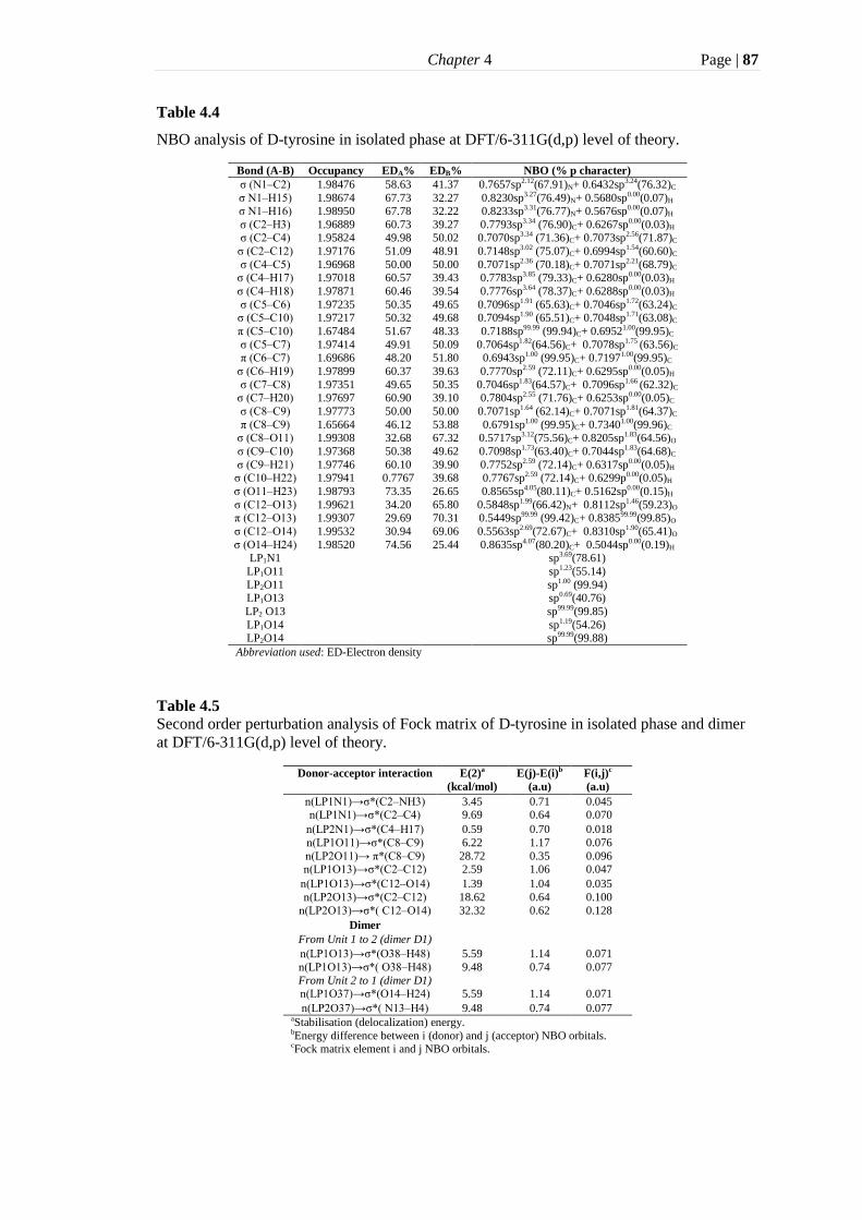
Chapter 4 Page | 87

Table 4.4

NBO analysis of D-tyrosine in isolated phase at DFT/6-311G(d,p) level of theory.

Bond (A-B) Occupancy EDA% EDB% NBO (% p character)

σ (N1‒C2) 1.98476 58.63 41.37 0.7657sp2.12(67.91)N+ 0.6432sp3.24(76.32)C

σ N1‒H15) 1.98674 67.73 32.27 0.8230sp3.27(76.49)N+ 0.5680sp0.00(0.07)H σ N1‒H16) 1.98950 67.78 32.22 0.8233sp3.31(76.77)N+ 0.5676sp0.00(0.07)H

σ (C2‒H3) 1.96889 60.73 39.27 0.7793sp3.34 (76.90)C+ 0.6267sp0.00(0.03)H σ (C2‒C4) 1.95824 49.98 50.02 0.7070sp3.34 (71.36)C+ 0.7073sp2.56(71.87)C

σ (C2‒C12) 1.97176 51.09 48.91 0.7148sp3.02 (75.07)C+ 0.6994sp1.54(60.60)C

σ (C4‒C5) 1.96968 50.00 50.00 0.7071sp2.36 (70.18)C+ 0.7071sp2.21(68.79)C σ (C4‒H17) 1.97018 60.57 39.43 0.7783sp3.85 (79.33)C+ 0.6280sp0.00(0.03)H

σ (C4‒H18) 1.97871 60.46 39.54 0.7776sp3.64 (78.37)C+ 0.6288sp0.00(0.03)H

σ (C5‒C6) 1.97235 50.35 49.65 0.7096sp1.91 (65.63)C+ 0.7046sp1.72(63.24)C σ (C5‒C10) 1.97217 50.32 49.68 0.7094sp1.90 (65.51)C+ 0.7048sp1.71(63.08)C

π (C5‒C10) 1.67484 51.67 48.33 0.7188sp99.99 (99.94)C+ 0.69521.00(99.95)C

σ (C5‒C7) 1.97414 49.91 50.09 0.7064sp1.82(64.56)C+ 0.7078sp1.75 (63.56)C π (C6‒C7) 1.69686 48.20 51.80 0.6943sp1.00 (99.95)C+ 0.71971.00(99.95)C

σ (C6‒H19) 1.97899 60.37 39.63 0.7770sp2.59 (72.11)C+ 0.6295sp0.00(0.05)H

σ (C7‒C8) 1.97351 49.65 50.35 0.7046sp1.83(64.57)C+ 0.7096sp1.66 (62.32)C σ (C7‒H20) 1.97697 60.90 39.10 0.7804sp2.55 (71.76)C+ 0.6253sp0.00(0.05)C

σ (C8‒C9) 1.97773 50.00 50.00 0.7071sp1.64 (62.14)C+ 0.7071sp1.81(64.37)C

π (C8‒C9) 1.65664 46.12 53.88 0.6791sp1.00 (99.95)C+ 0.73401.00(99.96)C σ (C8‒O11) 1.99308 32.68 67.32 0.5717sp3.12(75.56)C+ 0.8205sp1.83(64.56)O

σ (C9‒C10) 1.97368 50.38 49.62 0.7098sp1.73(63.40)C+ 0.7044sp1.83(64.68)C

σ (C9‒H21) 1.97746 60.10 39.90 0.7752sp2.59 (72.14)C+ 0.6317sp0.00(0.05)H σ (C10‒H22) 1.97941 0.7767 39.68 0.7767sp2.59 (72.14)C+ 0.6299p0.00(0.05)H

σ (O11‒H23) 1.98793 73.35 26.65 0.8565sp4.05(80.11)C+ 0.5162sp0.00(0.15)H

σ (C12‒O13) 1.99621 34.20 65.80 0.5848sp1.99(66.42)N+ 0.8112sp1.46(59.23)O π (C12‒O13) 1.99307 29.69 70.31 0.5449sp99.99 (99.42)C+ 0.838599.99(99.85)O

σ (C12‒O14) 1.99532 30.94 69.06 0.5563sp2.69(72.67)C+ 0.8310sp1.90(65.41)O

σ (O14‒H24) 1.98520 74.56 25.44 0.8635sp4.07(80.20)C+ 0.5044sp0.00(0.19)H LP1N1 sp3.69(78.61)

LP1O11 sp1.23(55.14)

LP2O11 sp1.00 (99.94) LP1O13 sp0.69(40.76)

LP2 O13 sp99.99(99.85)

LP1O14 sp1.19(54.26) LP2O14 sp99.99(99.88)

Abbreviation used: ED-Electron density

Table 4.5

Second order perturbation analysis of Fock matrix of D-tyrosine in isolated phase and dimer

at DFT/6-311G(d,p) level of theory.

Donor-acceptor interaction E(2)a

(kcal/mol)

E(j)-E(i)b

(a.u)

F(i,j)c

(a.u)

n(LP1N1)→σ*(C2‒NH3) 3.45 0.71 0.045 n(LP1N1)→σ*(C2‒C4) 9.69 0.64 0.070

n(LP2N1)→σ*(C4‒H17) 0.59 0.70 0.018

n(LP1O11)→σ*(C8‒C9) 6.22 1.17 0.076

n(LP2O11)→ π*(C8‒C9) 28.72 0.35 0.096 n(LP1O13)→σ*(C2‒C12) 2.59 1.06 0.047

n(LP1O13)→σ*(C12‒O14) 1.39 1.04 0.035

n(LP2O13)→σ*(C2‒C12) 18.62 0.64 0.100

n(LP2O13)→σ*( C12‒O14) 32.32 0.62 0.128

Dimer

From Unit 1 to 2 (dimer D1)

n(LP1O13)→σ*(O38‒H48) 5.59 1.14 0.071

n(LP1O13)→σ*( O38‒H48) 9.48 0.74 0.077

From Unit 2 to 1 (dimer D1)

n(LP1O37)→σ*(O14‒H24) 5.59 1.14 0.071

n(LP2O37)→σ*( N13‒H4) 9.48 0.74 0.077 aStabilisation (delocalization) energy. bEnergy difference between i (donor) and j (acceptor) NBO orbitals. cFock matrix element i and j NBO orbitals.

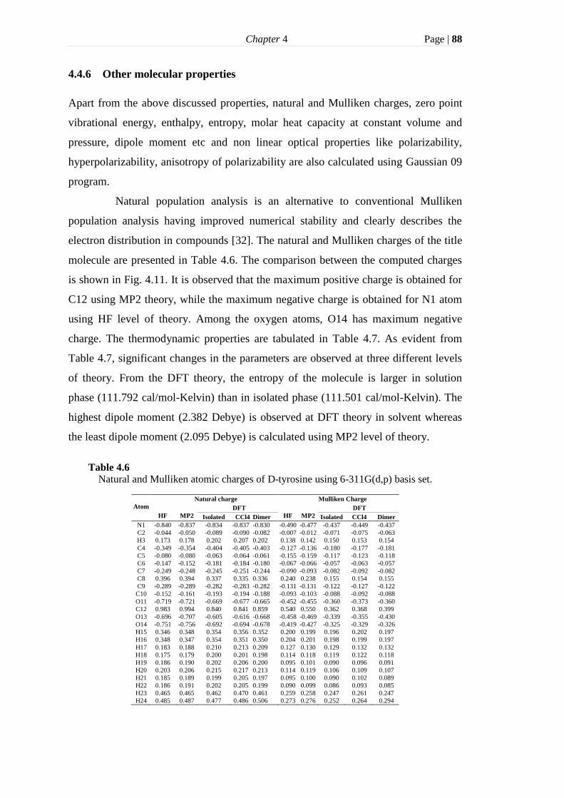
Chapter 4 Page | 88

4.4.6 Other molecular properties

Apart from the above discussed properties, natural and Mulliken charges, zero point

vibrational energy, enthalpy, entropy, molar heat capacity at constant volume and

pressure, dipole moment etc and non linear optical properties like polarizability,

hyperpolarizability, anisotropy of polarizability are also calculated using Gaussian 09

program.

Natural population analysis is an alternative to conventional Mulliken

population analysis having improved numerical stability and clearly describes the

electron distribution in compounds [32]. The natural and Mulliken charges of the title

molecule are presented in Table 4.6. The comparison between the computed charges

is shown in Fig. 4.11. It is observed that the maximum positive charge is obtained for

C12 using MP2 theory, while the maximum negative charge is obtained for N1 atom

using HF level of theory. Among the oxygen atoms, O14 has maximum negative

charge. The thermodynamic properties are tabulated in Table 4.7. As evident from

Table 4.7, significant changes in the parameters are observed at three different levels

of theory. From the DFT theory, the entropy of the molecule is larger in solution

phase (111.792 cal/mol-Kelvin) than in isolated phase (111.501 cal/mol-Kelvin). The

highest dipole moment (2.382 Debye) is observed at DFT theory in solvent whereas

the least dipole moment (2.095 Debye) is calculated using MP2 level of theory.

Table 4.6 Natural and Mulliken atomic charges of D-tyrosine using 6-311G(d,p) basis set.

Atom

Natural charge Mulliken Charge

HF

MP2

DFT

HF

MP2

DFT

Isolated CCl4 Dimer Isolated CCl4 Dimer

N1 -0.840 -0.837 -0.834 -0.837 -0.830 -0.490 -0.477 -0.437 -0.449 -0.437

C2 -0.044 -0.050 -0.089 -0.090 -0.082 -0.007 -0.012 -0.071 -0.075 -0.063

H3 0.173 0.178 0.202 0.207 0.202 0.138 0.142 0.150 0.153 0.154

C4 -0.349 -0.354 -0.404 -0.405 -0.403 -0.127 -0.136 -0.180 -0.177 -0.181

C5 -0.080 -0.080 -0.063 -0.064 -0.061 -0.155 -0.159 -0.117 -0.123 -0.118

C6 -0.147 -0.152 -0.181 -0.184 -0.180 -0.067 -0.066 -0.057 -0.063 -0.057

C7 -0.249 -0.248 -0.245 -0.251 -0.244 -0.090 -0.093 -0.082 -0.092 -0.082

C8 0.396 0.394 0.337 0.335 0.336 0.240 0.238 0.155 0.154 0.155

C9 -0.289 -0.289 -0.282 -0.283 -0.282 -0.131 -0.131 -0.122 -0.127 -0.122

C10 -0.152 -0.161 -0.193 -0.194 -0.188 -0.093 -0.103 -0.088 -0.092 -0.088

O11 -0.719 -0.721 -0.669 -0.677 -0.665 -0.452 -0.455 -0.360 -0.373 -0.360

C12 0.983 0.994 0.840 0.841 0.859 0.540 0.550 0.362 0.368 0.399

O13 -0.696 -0.707 -0.605 -0.616 -0.668 -0.458 -0.469 -0.339 -0.355 -0.430

O14 -0.751 -0.756 -0.692 -0.694 -0.678 -0.419 -0.427 -0.325 -0.329 -0.326

H15 0.346 0.348 0.354 0.356 0.352 0.200 0.199 0.196 0.202 0.197

H16 0.348 0.347 0.354 0.351 0.350 0.204 0.201 0.198 0.199 0.197

H17 0.183 0.188 0.210 0.213 0.209 0.127 0.130 0.129 0.132 0.132

H18 0.175 0.179 0.200 0.201 0.198 0.114 0.118 0.119 0.122 0.118

H19 0.186 0.190 0.202 0.206 0.200 0.095 0.101 0.090 0.096 0.091

H20 0.203 0.206 0.215 0.217 0.213 0.114 0.119 0.106 0.109 0.107

H21 0.185 0.189 0.199 0.205 0.197 0.095 0.100 0.090 0.102 0.089

H22 0.186 0.191 0.202 0.205 0.199 0.090 0.099 0.086 0.093 0.085

H23 0.465 0.465 0.462 0.470 0.461 0.259 0.258 0.247 0.261 0.247

H24 0.485 0.487 0.477 0.486 0.506 0.273 0.276 0.252 0.264 0.294

Chapter 4 Page | 89

Fig. 4.11 Comparison of the natural and Mulliken charges of D-tyrosine.

Table 4.7 Theoretical computed zero point vibrational energy (kcal mol

-1), thermal energy (kcal mol

-1),

entropy (cal mol-1

K-1

), enthalpy (kcal mol-1

), molar heat capacity at constant volume and

pressure (cal mol-1

K-1

) and dipole moment (Debye) of D-tyrosine molecule.

Parameters

HF

MP2

DFT

Isolated CCl4

Zero-point vibrational energy 130.285 121.733 121.265 121.161

Thermal Energy 137.627 129.663 129.005 128.931

Enthalpy 138.15 130.200 129.54 129.466

Entropy 109.193 112.708 111.501 111.792

Molar heat capacity at constant volume (Cv) 43.661 47.595 46.826 46.879

Molar heat capacity at constant pressure (Cp) 45.62 49.56 48.79 48.85

Dipole moment 2.2511 2.095 2.1361 2.382

Table 4.8

Calculated components of polarizability (a.u.), first order hyperpolarizability β(a.u.), mean

polarizability ‹α› (a.u.), anisotropy of the polarizability γ (a.u.) and the mean first order

hyperpolarizability β0 (esu, 1 a.u.=8.639 x 10–33

esu) of D-tyrosine in isolated phase.

DFT/6-311G(d,p)

αxx 158.82 βxxx 397.67

αxy 4.04 βxxy 41.71

αyy 113.01 βxyy -23.72

αxz -10.51 βyyy 9.44

αyz 8.66 βxxz -66.34

αzz 70.18 βxyz -23.89

‹ α › 114.00 βyyz -33.54

γ 80.624 βxzz 8.35

βyzz 16.70

βzzz -51.54

β0 (esu) 3.6 x 10–30

Chapter 4 Page | 90

The NLO properties of D-tyrosine are shown in Table 4.8. The computation of

polarizabilities and hyperpolarizabilities of the organic compounds are of great

significance to study the phenomenon induced by intermolecular interactions and

non–linear optical effects. The mean first order hyperpolarizability of D-tyrosine is

found 3.6 x 10–30

esu, which is about 9.7 times greater than the value for urea (β0 =

0.3728 x 10–30

esu) [33]. The high value of first order hyperpolarizability reflects the

non-linear property of a molecule.

4.5 Conclusions

The geometrical parameters of D-tyrosine molecule are computed and found to be in

agreement with the XRD data. The solvent environment has slightly affected the

geometrical parameters as marginal differences between RMS and MAD values for

isolated molecule and solution phases are observed. The experimental and theoretical

vibrational studies of D-tyrosine have been carried out. In general, good agreement

between experimental and calculated anharmonic frequencies has been observed. The

computed anharmonic frequencies are closer to matrix isolation FTIR bands. The

RMS and MAD values indicate that VSCF and CC-VSCF level of theory have

performed better anharmonic corrections than DFT, but the computational cost for the

former is very high. The DFT computed frequencies in gas and solution phases have

not shown any significant differences between their RMS values. It can be therefore

concluded that DFT approach in isolated and solution phases shows good

performance with equal accuracy and none of them can be considered superior for D-

tyrosine molecule. Signification stabilization of the dimer structure of D-tyrosine

molecule is also observed from the NBO analysis. From the calculation of coupling

strength, it is observed that mode-mode coupling between normal modes involving

displacements of the same atoms is typically stronger. The experimental and

theoretical UV-Vis spectra of D-tyrosine are also found in well agreement with each

other. From MEP analysis of D-tyrosine molecule, it is concluded that nitrogen atom

is more electrophilic than oxygen atoms, whereas the hydrogen atoms attached to

oxygen atoms are nucleophilic.

Chapter 4 Page | 91

References

[1]. G.A. Young, S. Kendall, A.M. Brownjohn, Amino Acids 6 (1994) 283–293.

[2]. L.I. Grace, R. Cohen, T.M. Dunn, D.M. Lubman, M.S. de Vries, J. Mol.

Spectrosc. 215 (2002) 204–219.

[3]. S. Kecel , A.E. Ozel, S. Akyuz , S. Celik, G. Agaeva, J. Mol. Struct. 993

(2011) 349–356.

[4]. R. Ramaekers, J. Pajak, M. Rospenk, G. Maes, Spectrochim. Acta A 61

(2005) 1347–1356.

[5]. A.K. Ojha, Chem. Phys. 340 (2007) 69–78.

[6]. S.J. Martinez, J.C. Alfano, D.H. Levy, J. Mol. Spectrosc. 156 (1992) 421–

430.

[7]. C.D. Contreras, A.E. Ledesma, H.E. Lanus, J. Zinczuk, S.A. Brandan, Vib.

Spectrosc. 57 (2011) 108–115.

[8]. B. Hernandez, F. Pfluger, A. Adenier, S.G. Kruglik, M. Ghomi, J. Phys.

Chem. B 114, (2010) 15319–15330.

[9]. J.N. Li, M. Pu, D.C. Fang, M. Wei, J. He, D.G. Evans, J. Mol. Struct. 1015

(2012) 106–111

[10]. Y. Huang, M. Shi, S. Zhao, H. Liang, J. Chromatogr. B 879 (2011) 3203–

3207.

[11]. P. Seidler, T. Kaga, K. Yagi, O. Christiansen, K. Hirao, Chem. Phys. Lett.

483 (2009) 138–142.

[12]. Barone, J. Chem. Phy. 122 (2005) 014108–014118.

[13]. M.J. Frisch, G.W. Trucks, H.B. Schlegel, G.E. Scuseria, et. al., Gaussian 09,

Revision D.01, Gaussian, Inc., Wallingford CT, 2009

[14]. E. Cances, B. Mennucci, J. Tomasi, J. Chem. Phys. 107 (1997) 3032–3041.

[15]. M.W. Schmidt, K.K. Baldridge, J.A. Boatz, S.T. Elbert, M.S. Gordon, et. al.,

J. Comput. Chem. 14 (1993) 1347–1363.

[16]. M.H. Jamroz, Vibrational Energy Distribution Analysis VEDA 4, Warsaw,

2004.

[17]. N.M.O. Boyle, A.L. Tenderholt, K.M. Langer, J. Comput. Chem. 29 (2008)

839–845.

[18]. E. D. Glendening, A. E. Reed, J. E. Carpenter, F. Weinhold, NBO Version

3.1.

[19]. A. Leahey, M.M. Olmstead, Private Communication (2001).

Chapter 4 Page | 92

[20]. A. Mostad, H.M. Nissen, C. Romming, Acta Chem. Scand. 26 (1972) 3819–

3833.

[21]. T. Rasheed, S. Ahmad, Vib. Spectrosc. 56 (2011) 51–59.

[22]. Y. Miller, G.M. Chaban, R.B. Gerber, J. Phys. Chem. A 109 (2005) 6565–

6574.

[23]. G. Socrates, Infrared and Raman Characteristic Group frequencies, Third

Edition, Wiley Interscience Publications, New York, 1980.

[24]. A. Abbas, H. Gokce, S. Bahceli, M.M. Naseer, J. Mol. Struct. 1075 (2014)

352–364.

[25]. G. Zhu, X. Zhu, Q. Fan, X. Wan, Spectrochim. Acta A 78 (2011) 1187–

1195.

[26]. N.P.G. Roeges, A Guide to the Complete Interpretation of Infrared Spectra

of Organic Structures, Wiley, New York (1994).

[27]. R.M. Tovar, K.P. Johnson, K. Ashline, J.M. Seminario, Int. J. Quantum

Chem. 108 (2008) 1546–1554.

[28]. A.M. Asiri, M. Karabacak, M. Kurt, K.A. Alamry, Spectrochim. Acta A 82

(2011) 444–455.

[29]. H. Galla, N. Issaoui, M. Govindarajan, H.T. Flakus, M.H. Jamroz, B. Oujia,

J. Mol. Struct. 1059 (2014) 132–143.

[30]. A. E. Reed, L. A. Curtiss, F. Weinhold, Chem. Rev. 88 (1988) 899–926.

[31]. F. Weinhold, C. R. Landis, Chemistry Education: Research and Practice in

Europe, 2 (2001) 91–104.

[32]. A.E. Reed, R.B. Weinstock, F. Weinhold, J. Chem. Phys. 83 (1985)

735‒746.

[33]. M.J. Alam, S. Ahmad, Spectrochim. Acta A 136 (2015) 961–978.

5 Structural, vibrational and electronic studies of 4–hydroxy–7–

methyl–1,8–naphthyridine–3–carboxylic acid

5.1 Introduction

Naphthyridines are the molecules in which two nitrogen atoms are substituted into a

naphthalene framework in a variety of patterns. The naphthyridines and their

derivatives are important due to their broad spectrum of pharmaceutical and medical

applications. For example, 1,8–naphthyridine derivatives have medicinal properties,

such as anti–HIV, anticancer, anti–inflammatory, antimalarial, antibacterial,

antiprotozoals, antimycobacterial, and antiplatelet [1‒10]. Many 1,8–naphthyridine

derivatives find their applications in controlling bacterial disorders and in treatment of

allergic chronic obstructive lung diseases [11–13]. In addition, 1,8–naphthyridine

derivatives have been reported to be excellent fluorescent markers of nucleic acids

[14,15].

The knowledge of the structures and spectra of naphthyridine derivatives are

helpful in understanding the biological processes and mechanism of action of drugs.

Therefore, the aim of the present chapter is to investigate the molecular structure,

vibrational and electronic spectra and other molecular properties of the 4–hydroxy–7-

methyl–1,8–naphthyridine–3–carboxylic acid (HMNC) molecule. The anharmonic

frequency calculations for HMNC are performed using VPT2 [16], VSCF [17] and

CC–VSCF [18,19] methods. The intermolecular interactions are explained on the

basis of the harmonic frequency calculations for the dimer structure of the title

molecule. The theoretical calculations particularly the anharmonic frequencies

simulations are invaluable tools for reliable assignments of the vibrational modes [20–

23]. The electronic absorption spectra in water and ethanol solution are also simulated

using integral equation formalism of the polarisation continuum model (IEF–PCM).

The computed results are compared with the experimental data (FTIR, FT–Raman and

Chapter 5 Page | 94

UV–Vis). NBO, MEP mapping, HOMO–LUMO, charge analysis and few other

molecular properties of HMNC are also discussed.

5.2 Experimental details

The compound, HMNC, was obtained from Sigma Aldrich chemicals company, USA

and was used as such for recording of the FTIR, FT–Raman and UV–Vis spectra. The

FTIR spectrum was recorded at room temperature in the region 4000–400 cm–1

on

Bruker Tensor 37 spectrometer, with a spectral resolution of 2 cm–1

, using KBr pellet

technique. To increase the signal–to–noise ratio, a minimum of 32 scans were

accumulated. The FT–Raman spectrum was recorded in the region 4000–50 cm–1

on

Bruker RFS 27 FT–Raman spectrometer, with a spectral resolution of 2 cm–1

. UV–Vis

spectra of HMNC in water and ethanol solvents were recorded in the region 800‒200

nm on Lambda 950 UV–Vis–NIR spectrophotometer.

5.3 Computational details

The theoretical calculations for HMNC molecule were performed using HF, DFT and

MP2 level of theory with 6–311G(d,p) basis set. The electron correlations were

included using the Becke's three–parameter hybrid exchange functional (B3) and the

Lee Yang Par (LYP) correlation functional [24–27]. The optimized structural

parameters of the molecule in the ground state were obtained under the tight

convergence criterion. Subsequently, the harmonic and anharmonic vibrational

frequencies along with IR and Raman activities were calculated. Raman activities

were converted into intensities using the equation (3.1) described in chapter 3.

Harmonic frequencies were also calculated for the dimer structure of the molecule

using DFT level of theory. Anharmonic corrections in vibrational frequencies were

obtained by the VPT2 approach using Gaussian 09 package [28], as well as

VSCF/2MR–QFF and CC–VSCF methods implemented in GAMESS–US package

[29]. The vibrational assignments were made using Veda 4 program [30] and visual

inspection of the atomic displacements in Gauss–View. The combination and

overtone bands in the FTIR spectrum are also assigned. In order to know the coupling

between pair of modes, the magnitudes of mode–mode coupling are estimated. The

2MR–QFF potential energy function was used for calculating anharmonic mode–

mode coupling strengths [31,32]. NBO analysis is reported at DFT/6–311G(d,p) level

Chapter 5 Page | 95

of theory using NBO 3.1 program [33]. Electronic spectra in the water and ethanol

solutions were simulated using the IEF–PCM model at TD–B3LYP/6–311++G(d,p)

level of theory. The chemical behaviour and reactivity of HMNC were investigated

using MEP and HOMO–LUMO analysis at DFT/6–311G(d,p) level of theory. Other

molecular properties including charge analysis, thermodynamic and non linear optical

(NLO) properties are also calculated.

5.4 Results and discussions

5.4.1 Geometric structure

The optimized geometries of the monomer and dimer structure of HMNC are shown

in Fig. 5.1. The calculated structural parameters of the molecule are listed in Table

5.1. The optimized parameters are compared with the X–ray data of similar kind of

molecules. The DFT computed C–C bond lengths are nearly same in both monomer

and dimer structures. These do not show any effect of dimerization. It is observed that

most of the parameters computed at HF, DFT and MP2 levels of theory are deviated

from the literature [34–36]. The deviation may be due to the fact that these parameters

have been simulated in isolated phase, while the XRD data [34–36] has been recorded

in solid phase in the presence of intra and inter- molecular interactions. It is observed

from Table 5.1 that O15‒H23 and C13=O14 bond lengths are larger in dimer than the

monomer. The elongation of O15‒H23 bond length in dimer is a result of the

intermolecular hydrogen bonding. The lengthening of the C13=O14 bond in HMNC

upon dimerization may be due to the electron withdrawing nature of the carboxylic

group. The shortening of the C13‒O15 bond in dimer may be due to the redistribution

of partial charges on O15 atom. Comparing the bond lengths of HMNC with that of

1,8–naphthyridine molecule [35], it is observed that C–C and C–H bond lengths are

longer in HMNC. C–N bond lengths, except C8–N7, are shorter in HMNC than those

in 1,8–naphthyridine molecule. Similarly, the predicted C–O and C=O bond lengths

of HMNC are longer and shorter respectively than those of nalidixic acid [34]. High

dipole moment, 2.2747 Debye, calculated for HMNC at B3LYP favours the formation

of the hydrogen bonded dimer. The calculated O···H bond lengths and O‒H···O bond

angles are 1.670 Å and 179.1◦ respectively. Besides, the value of the dipole moment

(0.0001 Debye) confirms the centrosymmetry of the dimer molecule.

Chapter 5 Page | 96

Fig. 5.1 Optimized structures of the monomer and dimer form of HMNC molecule.

Table 5.1

Optimized geometrical parameters of of HMNC using 6–311G(d,p) basis set.

Bond length

(Å)

DFT

HF

MP2

XRDa

XRDb

XRDc

Bond Angle

(◦)

DFT

HF

MP2

XRDa

XRDb

XRDc Monomer Dimer Monomer Dimer

O1–C2 1.330 1.331 1.314 1.337 1.261 1.210 C2–O1–H16 107.2 107.3 109.9 105.8

O1–H16 0.988 0.984 0.953 0.981 O1–C2–C3 123.6 123.8 124.4 124.5 122.9 127.1

C2–C3 1.400 1.400 1.383 1.393 1.436 1.350 1.426 O1–C2–C11 118.4 118.1 117.5 117.8 121.9 119.1

C2–C11 1.423 1.423 1.418 1.427 1.445 1.409 1.472 C3–C2–C11 118.0 118.0 118.1 117.7 115.2 119.3 113.8

C3–C4 1.423 1.425 1.420 1.426 1.384 1.395 1.376 C2–C3–C4 118.1 117.9 117.7 118.7 118.8 118.8 120.3 C3–C13 1.459 1.458 1.463 1.470 1.461 1.488 C2–C3–C13 118.9 120.2 120.0 118.7 121.0 119.8

C4–N5 1.308 1.307 1.286 1.316 1.316 1.313 1.335 C4–C3–C13 123.0 121.9 122.4 122.6 120.2 119.8

C4–H17 1.086 1.086 1.075 1.088 0.95 0.96 C3–C4–N5 125.3 125.4 125.4 125.2 125.3 125.2 124.6 N5–C6 1.367 1.368 1.356 1.371 1.387 1.369 1.326 C3–C4–H17 117.9 117.7 117.9 118.2 122.8

C6–N7 1.355 1.355 1.347 1.363 1.353 1.362 1.417 N5–C4–H17 116.8 116.9 116.7 116.7 112.1

C6–C11 1.424 1.424 1.402 1.421 1.407 1.418 1.401 C4–N5–C6 117.4 117.4 117.7 116.7 119.7 116.7 117.9 N7–C8 1.320 1.321 1.296 1.326 1.325 1.314 1.353 N5–C6–N7 115.9 115.9 116.0 114.9 116.6 115.3 117.6

C8–C9 1.422 1.422 1.424 1.424 1.406 1.400 1.403 N5–C6–C11 122.7 122.6 122.6 123.2 118.9 122.1 123.5

C8–C12 1.506 1.506 1.505 1.506 1.522 N7–C6–C11 121.5 121.5 121.5 121.9 124.5 122.6 118.9 C9–C10 1.369 1.369 1.352 1.376 1.361 1.357 1.363 C6–N7–C8 119.2 119.2 119.5 118.5 117.1 116.9 121.0

C9–H18 1.084 1.084 1.074 1.087 0.97 0.98 N7–C8–C9 122.9 122.8 123.1 123.0 123.2 125.0 119.1

C10–C11 1.413 1.413 1.415 1.415 1.418 1.413 N7–C8–C12 117.2 117.2 117.6 117.2 116.4 C10–H19 1.083 1.083 1.073 1.085 0.99 C9–C8–C12 119.9 119.9 119.3 119.8 120.3

C12–H20 1.095 1.095 1.087 1.095 C8–C9–C10 119.2 119.2 118.7 119.7 119.4 118.6 122.4

C12–H21 1.095 1.095 1.087 1.095 C8–C9–H18 119.8 119.8 119.8 119.5 120.9 C12–H22 1.089 1.089 1.080 1.091 C10–C9–H18 121.0 121.0 121.5 120.8 120.5 118.6

C13–O14 1.228 1.249 1.199 1.226 1.230 1.203 C9–C10–C11 118.7 118.7 118.8 118.0 119.7 119.4

C13–O15 1.343 1.314 1.319 1.342 1.323 1.335 C9–C10–C19 121.8 121.8 121.7 122.3 121.7 O15–H23 0.969 1.00 0.946 0.968 0.78 C11–C10–C19 119.4 119.5 119.5 119.7 119.2

C2–C11–C6 118.5 118.6 118.6 118.6 122.0 117.8 118.9

C2–C11–C10 122.9 122.9 122.9 122.4 121.9 124.7 121.2 H‒bond lengths (Å) and angles (◦) C6–C11–C10 118.6 118.5 118.5 119.0 118.5 118.5 119.9

O∙∙∙H 1.670 C8–C12–H20 110.8 110.8 110.4 110.7

O–H∙∙∙O 179.1 C8–C12–H21 110.8 110.8 110.4 110.7

C8–C12–H22 109.6 109.6 109.8 109.2

H20–C12–H21 107.2 107.2 107.6 107.7 H20–C12–H22 109.1 109.1 109.3 109.2

H21–C12–H22 109.1 109.1 109.3 109.2

C3–C13–O14 123.9 121.7 124.0 123.8 124.0 126.4 C3–C13–O15 114.9 116.1 114.6 114.2 116.7 111.0

O14–C13–O15 121.2 122.3 121.4 122.0 119.3 122.6

C13–O15–H23 106.8 110.6 108.4 105.5

a=[34], b=[35], c=[36]

Chapter 5 Page | 97

5.4.2 Vibrational analysis

The molecule, HMNC, consists of 23 atoms and belongs to C1 point group.

Therefore, all the 63 vibrational modes of HMNC are active in both IR and Raman

spectra. Comparison between FT–IR and FT–Raman spectra of HMNC are shown in

Fig. 5.2 and Fig. 5.3 respectively. Comparison of the calculated frequencies at

harmonic level with the experimental data shows overestimation due to the neglect of

anharmonicity. In order to make accurate assignments of the experimental

wavenumbers, anharmonic correction is made to each vibrational frequency. Root

mean square (RMS) value shows that the VSCF (RMS=32) method yields better

anharmonic corrections in agreement with the experimental data. The VPT2 method

shows RMS value of 63, whereas the MP2 and HF levels of theory have 126 and 174

RMS values respectively. The calculated wavenumbers, FT–IR and FT–Raman

frequencies along with their intensities and vibrational assignments are given in Table

5.2. The histogram indicating the deviations of predicted anharmonic wavenumbers

from the experimental ones is shown in shown in Fig. 5.4. It can be seen from the

histogram that the anharmonic frequency deviation is highest for mode 1 calculated

using HF level of theory. The average percentage error in the regions above 1700 cm–

1 and 1700–900 cm

–1 have been found 1.56 and 1.09% respectively in VSCF method

as compared to 1.78, 1.10% and 3.03, 1.24% respectively for CC–VSCF and VPT2

levels of theory. In the region below 900 cm–1

, VPT2 level of theory shows less

percentage error (2.38%) than the VSCF (3.27%) and CC–VSCF (3.5.6%) methods.

Both HF and MP2 levels of theory show large error in all the three regions. The

carboxylic acid group in HMNC is involved in intermolecular hydrogen bonding. As

can be seen from frequency computations in the dimer, these intermolecular

interactions show significant changes in frequencies of many vibrational modes.

Mode pair coupling strengths in 2MR–QFF representations and the modes having

coupling strengths greater than 15 cm–1

are shown in Fig. 5.5 and Fig. 5.6

respectively. It is clear from Fig. 5.5 that most of the normal mode pairs have very

low coupling strength except some pairs which show medium to high coupling

strengths. From Fig. 5.6, high coupling strengths, greater than 350 cm–1

, are observed

between the mode pairs (6,61), (7,61) and (8,61). The Coupling strengths between

some important pair of modes are also presented in Fig. 5.7. The combination and

overtone bands are also assigned in the FTIR spectrum of HMNC in the region 2850–

Chapter 5 Page | 98

2340 cm–1

and are tabulated (Table 5.2). The weak bands observed at 2853, 2731 and

2346 cm–1

and at 2885, 2787 and 2375 cm–1

are assigned to overtone and combination

bands respectively. These combination bands may also provide a more unique

identification in HMNC.

Fig. 5.2 Comparison of the experimental FTIR and computed anharmonic spectra of

HMNC using 6–311G(d,p) basis set.

Fig. 5.3 Comparison of the experimental FT-Raman and computed Raman spectra of

HMNC using 6–311G(d,p) basis set.

Chapter 5 Page | 99

Table 5.2

Comparison of the experimental and computed vibrational frequencies of HMNC molecule using 6–311G(d,p) basis set.

M

Experimental B3LYP MP2 HF

FTIR

FT–

Raman

Har

A

R

Ra

Dimer

VPT2 VSCF CC–

VSCF

Aa

Har

VPT2 A

R Har

VPT2 A

R Assignment (PED>5%)

1 3249ms 3765 134.4 53.1 3580 3349 3373 139.1 8.1 3226, 3141 3812 3625 146.6 41.0 4118 3947 205.5 22.4 ν [O15–H23] (100)

2 3195ms 3360 446.6 27.9 3047 3144 3167 65.4 39.7 3426, 3424 3500 3230 384.0 30.3 3936 3724 397.3 8.2 ν [O1–H16] (99)

3 3073s 3074s 3202 4.9 54.5 3072 3062 3072 9.3 67.1 3203, 3203 3239 3109 3.8 50.2 3373 3253 4.8 37.6 ν [C9–H18] (83) + ν [C10–H19] (16)

4 3179 6.2 52.9 3030 2984 2999 0.8 47.4 3180, 3180 3214 3080 4.4 48.2 3348 3229 7.3 41.7 ν [C10–H19] (84) + ν [C9–H18] (16)

5 3163 5.6 50.7 3029 2969 2975 5.3 36.8 3166,3166 3208 3083 4.2 47.8 3345 3214 6.1 34.8 ν [C4–H17] (99)

6 2996ms 2992m 3142 6.3 34.1 2990 2936 2915 16.3 4.8 3143,3143 3198 3056 3.4 29.1 3289 3177 10.0 27.7 νas[CH3] (84)

7 3077 14.9 67.3 2931 2920 2882 8.8 40.4 3077, 3077 3149 3014 12.4 53.4 3220 3074 23.9 48.2 νas [H21–C12–H20] [in CH3] (100)

8 2921ms 2929s 3028 14.1 191.2 2924 2898 2878 11.9 168.3 3028,3028 3073 2977 16.3 142.3 3169 3059 20.4 109.4 νsy [CH3] (85)

2853w 2926 2846 2800 2789 2×1425

2885w 2976 2902 2874 2871 1545+1330

2786w 2868 2794 2757 2748 1425+1364

2731w 2811 2721 2708 2679 2×1364

2375w 2440 2395 2400 2379 1615+767

2346w 2413 2363 2308 2302 2×1174

9 1733vs 1719s 1732 398.3 231.2 1696 1753 1752 338.6 210.6 1691, 1666 1780 1748 327.0 295.7 1927 1893 617.1 83.1 ν [C13=O14] (65) + β [H23–O15–C13) (6) + β [C2–C3–C13] (6)

10 1615vs 1611vs 1657 329.3 122.1 1631 1616 1614 56.9 67.0 1654 1687 1650 223.9 300.3 1821 1784 661.0 112.7 ν [C2–C3+ C2–C11] (51) + β [H16–O1–C2] (16) + ν [C10–C11] (6)

11 1646 121.1 95.2 1605 1606 1604 196.8 191.8 1645 1656 1612 70.7 23.2 1811 1770 105.9 26.0 ν [C9–C10] (58) + β [H18–C9–C8 + H19–10–C11] (8) + ν [C8–N7 + C6–N7] (6)

12 1545s 1557s 1595 135.3 36.9 1557 1549 1546 93.6 62.8 1593, 1593 1612 1575 46.3 35.9 1760 1722 257.9 40.7 ν [C8–C9+ C6–C11] (36) + β [C3–C2–C11] (6) + ν [C4–N5 + C8–N7] (6)

13 1475vs 1478w 1516 119.6 106.1 1478 1491 1489 34.8 28.6 1529, 1511 1552 1511 91.3 194.6 1643 1608 48.7 8.1 ν [C2–C3 + C2–C11 + C3–C4 + C8–C9] (29) + β [H18–C9–C10 + H19–10–C11] (16)

14 1500 2.6 1.4 1462 1479 1480 10.9 51.8 1497,1490 1513 1472 11.5 61.9 1630 1602 110.5 23.9 β [H17–C4–N5] (44) + βas [CH3] (11) + ν [NC] (6)

15 1486 8.4 38.2 1450 1454 1453 9.1 14.0 1486, 1486 1500 1459 8.0 35.6 1603 1574 7.7 28.5 βas [CH3] (79) + τ [H20–C12–C8–C9 + H21–C12–C8–C9 + H22–C12–C8–C9] (22)

16 1446w 1469 19.1 20.7 1413 1451 1452 0.4 67.6 1450 1489 1441 21.2 792.4 1586 1553 10.8 75.7 β [H16–O1–C2] (25) + ν [N5–C4] (24) + ν [N7–C8] (6) + β [HCC] (6)

17 1463 22.6 163.2 1427 1401 1399 53.7 300.7 1461, 1460 1478 1426 13.5 12.9 1579 1549 3.0 43.6 β [H17–C4–N5] (58) + ν [C8–C9 + C3–C4] (8) ν [N5–C6 + N7–C8] (6)

18 1381s 1433 228.3 297.9 1399 1398 1397 135.7 661.1 1381,1374 1468 1422 26.2 216.6 1550 1522 385.5 95.3 ν [O1–C2 + O15–C13] (23) + β [O15–H23] (14) + ν [N7–C6 + N5–C4]

+ β [O14–C13–O15] (10) + ν [C13–C3 +C2–C11] (7)

19 1422 123.5 85.5 1390 1380 1377 24.1 66.5 1424,1423 1439 1406 226.2 23.5 1539 1494 63.6 228.7 β [N7–C6] (23) + β [HCN] (14) + ν [N5–C6] (8) + β [H16–O1–C2] (7)

+ β [HCC] (7)

20 1364s 1406 10.7 80.1 1370 1355 1347 491.9 18.6 1406,1406 1414 1381 9.3 8.8 1530 1502 9.1 12.8 umb.[CH3] (91)

21 1330ms 1325vs 1382 115.9 376.7 1347 1326 1324 15.9 158.3 1373,1369 1413 1375 99.4 283.3 1479 1437 156.1 78.9 ν [N7–C6] (26) + β [O1–H16] (27) + β [H19–C10–C11 + H17–C4–C3] (8)

+ ν [C9–C10 + C2–C11] (7)

22 1292w 1293m 1354 6.9 269.1 1321 1301 1298 16.0 89.0 1348,1347 1373 1346 33.2 12.8 1446 1416 16.8 456.8 ν [C8–C9 + C6–C11 + C4–C3] (17) + β [H19–C10–C11 + H17–C4–C3] (7)

+ β [N7–C6–N5] (6)

23 1326 17.9 67.8 1297 1266 1258 53.5 27.4 1303,1301 1345 1317 37.5 25.4 1423 1397 3.0 81.7 ν [N7–C8] (32) + β [CNC] (7) + β [H23–O15–C3 + H16–O1–C2] (6)

24 1243s 1250w 1273 17.8 79.3 1240 1242 1239 33.1 84.1 1275,1275 1293 1259 18.6 82.1 1362 1332 23.7 64.7 ν [O1–C2 + O15–C13] (11) + β [C2–C3–C13 + C2–C11–C10] (25)

+ ν [NC] (7) + β [HOC] (6)

25 1220sh 1221w 1258 37.9 24.6 1231 1218 1215 54.0 47.2 1250 1274 1249 10.8 12.2 1345 1314 158.2 25.2 ν [CC] (27) + β [H23–O15–C13] (10) + β [HCC] (11) + ν [NC] (7) + umb [CH3] (7)

26 1220 150.3 35.4 1192 1206 1204 35.1 11.8 1219,1218 1238 1207 154.0 42.6 1316 1290 256.4 11.6 ν [N–C] (23) + β [O15–H23] (10) + β [H18–C9] (10) + ν [CC] (9) + β [C6–N7–C8] (7)

+ β [C3–C2–C11] (6)

27 1174ms 1172w 1207 97.8 16.8 1182 1154 1152 45.7 17.8 1249 1217 1190 130.9 18.3 1283 1265 13.1 11.1 β [H19–C10] (20) + ν [N5–C6 + N7–C6] (14) + β [O15–H23] (13) + β [O15–C13] (11)

+ ν [C9–C10 + C10–C11] (7)

28 1142w 1146w 1165 256.3 42.6 1140 1130 1127 75.8 20.4 1188,1188 1173 1150 177.3 36.2 1234 1210 183.8 31.6 β [HC] (31) + ν [O15–C13] (20) + β [O15–H23] (17)

29 1106w 1107w 1110 77.1 28.2 1092 1057 1055 4.6 29.0 1117,1117 1111 1094 63.5 16.1 1185 1168 1.4 6.8 ν [OC] (43) + β [HCC] (23)

30 1044w 1058 3.1 0.9 1035 1053 1052 5.0 4.4 1058,1058 1060 1045 0.9 0.5 1157 1136 3.1 1.2 τ [H20–C12–C8–C9 + H21–C12–C8–C9 + H22–C12–C8–C9] (67) + roc [CH3] (16)

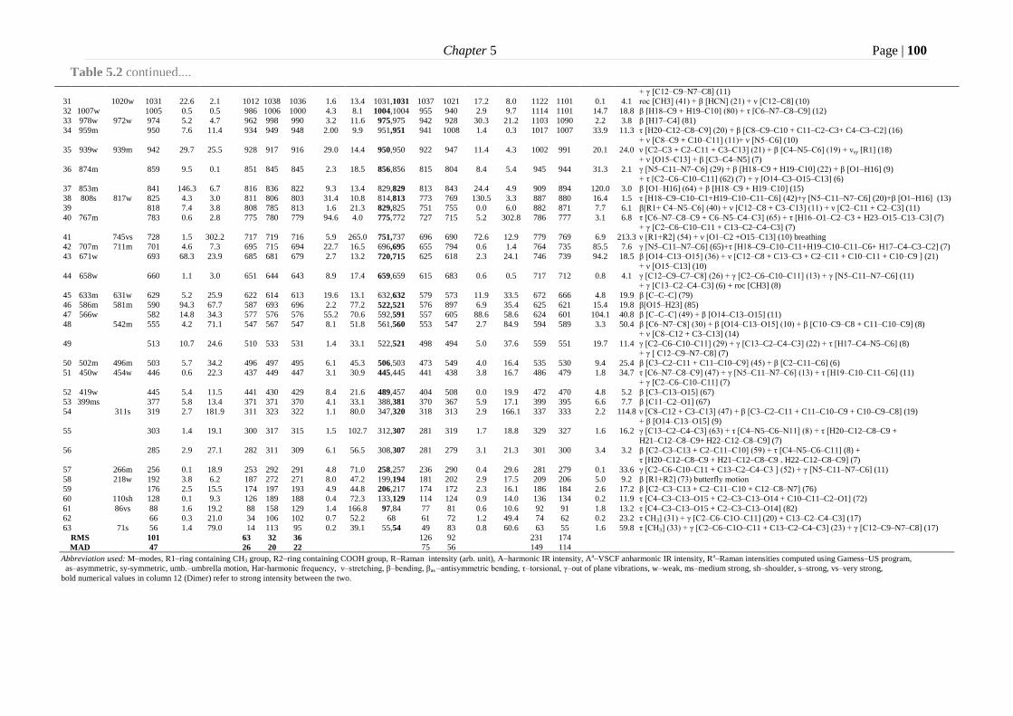
Chapter 5 Page | 100

+ γ [C12–C9–N7–C8] (11)

31 1020w 1031 22.6 2.1 1012 1038 1036 1.6 13.4 1031,1031 1037 1021 17.2 8.0 1122 1101 0.1 4.1 roc [CH3] (41) + β [HCN] (21) + ν [C12–C8] (10)

32 1007w 1005 0.5 0.5 986 1006 1000 4.3 8.1 1004,1004 955 940 2.9 9.7 1114 1101 14.7 18.8 β [H18–C9 + H19–C10] (80) + τ [C6–N7–C8–C9] (12)

33 978w 972w 974 5.2 4.7 962 998 990 3.2 11.6 975,975 942 928 30.3 21.2 1103 1090 2.2 3.8 β [H17–C4] (81)

34 959m 950 7.6 11.4 934 949 948 2.00 9.9 951,951 941 1008 1.4 0.3 1017 1007 33.9 11.3 τ [H20–C12–C8–C9] (20) + β [C8–C9–C10 + C11–C2–C3+ C4–C3–C2] (16)

+ ν [C8–C9 + C10–C11] (11)+ ν [N5–C6] (10)

35 939w 939m 942 29.7 25.5 928 917 916 29.0 14.4 950,950 922 947 11.4 4.3 1002 991 20.1 24.0 ν [C2–C3 + C2–C11 + C3–C13] (21) + β [C4–N5–C6] (19) + νsy [R1] (18)

+ ν [O15–C13] + β [C3–C4–N5] (7)

36 874m 859 9.5 0.1 851 845 845 2.3 18.5 856,856 815 804 8.4 5.4 945 944 31.3 2.1 γ [N5–C11–N7–C6] (29) + β [H18–C9 + H19–C10] (22) + β [O1–H16] (9)

+ τ [C2–C6–C10–C11] (62) (7) + γ [O14–C3–O15–C13] (6)

37 853m 841 146.3 6.7 816 836 822 9.3 13.4 829,829 813 843 24.4 4.9 909 894 120.0 3.0 β [O1–H16] (64) + β [H18–C9 + H19–C10] (15)

38 808s 817w 825 4.3 3.0 811 806 803 31.4 10.8 814,813 773 769 130.5 3.3 887 880 16.4 1.5 τ [H18–C9–C10–C1+H19–C10–C11–C6] (42)+γ [N5–C11–N7–C6] (20)+β [O1–H16] (13)

39 818 7.4 3.8 808 785 813 1.6 21.3 829,825 751 755 0.0 6.0 882 871 7.7 6.1 β[R1+ C4–N5–C6] (40) + ν [C12–C8 + C3–C13] (11) + ν [C2–C11 + C2–C3] (11)

40 767m 783 0.6 2.8 775 780 779 94.6 4.0 775,772 727 715 5.2 302.8 786 777 3.1 6.8 τ [C6–N7–C8–C9 + C6–N5–C4–C3] (65) + τ [H16–O1–C2–C3 + H23–O15–C13–C3] (7)

+ γ [C2–C6–C10–C11 + C13–C2–C4–C3] (7)

41 745vs 728 1.5 302.2 717 719 716 5.9 265.0 751,737 696 690 72.6 12.9 779 769 6.9 213.3 ν [R1+R2] (54) + ν [O1–C2 +O15–C13] (10) breathing

42 707m 711m 701 4.6 7.3 695 715 694 22.7 16.5 696,695 655 794 0.6 1.4 764 735 85.5 7.6 γ [N5–C11–N7–C6] (65)+τ [H18–C9–C10–C11+H19–C10–C11–C6+ H17–C4–C3–C2] (7)

43 671w 693 68.3 23.9 685 681 679 2.7 13.2 720,715 625 618 2.3 24.1 746 739 94.2 18.5 β [O14–C13–O15] (36) + ν [C12–C8 + C13–C3 + C2–C11 + C10–C11 + C10–C9 ] (21)

+ ν [O15–C13] (10)

44 658w 660 1.1 3.0 651 644 643 8.9 17.4 659,659 615 683 0.6 0.5 717 712 0.8 4.1 γ [C12–C9–C7–C8] (26) + γ [C2–C6–C10–C11] (13) + γ [N5–C11–N7–C6] (11)

+ γ [C13–C2–C4–C3] (6) + roc [CH3] (8)

45 633m 631w 629 5.2 25.9 622 614 613 19.6 13.1 632,632 579 573 11.9 33.5 672 666 4.8 19.9 β [C–C–C] (79)

46 586m 581m 590 94.3 67.7 587 693 696 2.2 77.2 522,521 576 897 6.9 35.4 625 621 15.4 19.8 β[O15–H23] (85)

47 566w 582 14.8 34.3 577 576 576 55.2 70.6 592,591 557 605 88.6 58.6 624 601 104.1 40.8 β [C–C–C] (49) + β [O14–C13–O15] (11)

48 542m 555 4.2 71.1 547 567 547 8.1 51.8 561,560 553 547 2.7 84.9 594 589 3.3 50.4 β [C6–N7–C8] (30) + β [O14–C13–O15] (10) + β [C10–C9–C8 + C11–C10–C9] (8)

+ ν [C8–C12 + C3–C13] (14)

49 513 10.7 24.6 510 533 531 1.4 33.1 522,521 498 494 5.0 37.6 559 551 19.7 11.4 γ [C2–C6–C10–C11] (29) + γ [C13–C2–C4–C3] (22) + τ [H17–C4–N5–C6] (8)

+ γ [ C12–C9–N7–C8] (7)

50 502m 496m 503 5.7 34.2 496 497 495 6.1 45.3 506,503 473 549 4.0 16.4 535 530 9.4 25.4 β [C3–C2–C11 + C11–C10–C9] (45) + β [C2–C11–C6] (6)

51 450w 454w 446 0.6 22.3 437 449 447 3.1 30.9 445,445 441 438 3.8 16.7 486 479 1.8 34.7 τ [C6–N7–C8–C9] (47) + γ [N5–C11–N7–C6] (13) + τ [H19–C10–C11–C6] (11)

+ γ [C2–C6–C10–C11] (7)

52 419w 445 5.4 11.5 441 430 429 8.4 21.6 489,457 404 508 0.0 19.9 472 470 4.8 5.2 β [C3–C13–O15] (67)

53 399ms 377 5.8 13.4 371 371 370 4.1 33.1 388,381 370 367 5.9 17.1 399 395 6.6 7.7 β [C11–C2–O1] (67)

54 311s 319 2.7 181.9 311 323 322 1.1 80.0 347,320 318 313 2.9 166.1 337 333 2.2 114.8 ν [C8–C12 + C3–C13] (47) + β [C3–C2–C11 + C11–C10–C9 + C10–C9–C8] (19)

+ β [O14–C13–O15] (9)

55 303 1.4 19.1 300 317 315 1.5 102.7 312,307 281 319 1.7 18.8 329 327 1.6 16.2 γ [C13–C2–C4–C3] (63) + τ [C4–N5–C6–N11] (8) + τ [H20–C12–C8–C9 +

H21–C12–C8–C9+ H22–C12–C8–C9] (7)

56 285 2.9 27.1 282 311 309 6.1 56.5 308,307 281 279 3.1 21.3 301 300 3.4 3.2 β [C2–C3–C13 + C2–C11–C10] (59) + τ [C4–N5–C6–C11] (8) +

τ [H20–C12–C8–C9 + H21–C12–C8–C9 + H22–C12–C8–C9] (7)

57 266m 256 0.1 18.9 253 292 291 4.8 71.0 258,257 236 290 0.4 29.6 281 279 0.1 33.6 γ [C2–C6–C10–C11 + C13–C2–C4–C3 ] (52) + γ [N5–C11–N7–C6] (11)

58 218w 192 3.8 6.2 187 272 271 8.0 47.2 199,194 181 202 2.9 17.5 209 206 5.0 9.2 β [R1+R2] (73) butterfly motion

59 176 2.5 15.5 174 197 193 4.9 44.8 206,217 174 172 2.3 16.1 186 184 2.6 17.2 β [C2–C3–C13 + C2–C11–C10 + C12–C8–N7] (76)

60 110sh 128 0.1 9.3 126 189 188 0.4 72.3 133,129 114 124 0.9 14.0 136 134 0.2 11.9 τ [C4–C3–C13–O15 + C2–C3–C13–O14 + C10–C11–C2–O1] (72)

61 86vs 88 1.6 19.2 88 158 129 1.4 166.8 97,84 77 81 0.6 10.6 92 91 1.8 13.2 τ [C4–C3–C13–O15 + C2–C3–C13–O14] (82)

62 66 0.3 21.0 34 106 102 0.7 52.2 68 61 72 1.2 49.4 74 62 0.2 23.2 τ CH3] (31) + γ [C2–C6–C1O–C11] (20) + C13–C2–C4–C3] (17)

63 71s 56 1.4 79.0 14 113 95 0.2 39.1 55,54 49 83 0.8 60.6 63 55 1.6 59.8 τ [CH3] (33) + γ [C2–C6–C1O–C11 + C13–C2–C4–C3] (23) + γ [C12–C9–N7–C8] (17)

RMS 101 63 32 36 126 92 231 174

MAD 47 26 20 22 75 56 149 114

Abbreviation used: M–modes, R1–ring containing CH3 group, R2–ring containing COOH group, R–Raman intensity (arb. unit), A–harmonic IR intensity, Aa–VSCF anharmonic IR intensity, Ra–Raman intensities computed using Gamess–US program,

as–asymmetric, sy-symmetric, umb.–umbrella motion, Har-harmonic frequency, ν–stretching, β–bending, βas –antisymmetric bending, τ–torsional, γ–out of plane vibrations, w–weak, ms–medium strong, sh–shoulder, s–strong, vs–very strong,

bold numerical values in column 12 (Dimer) refer to strong intensity between the two.

Table 5.2 continued....

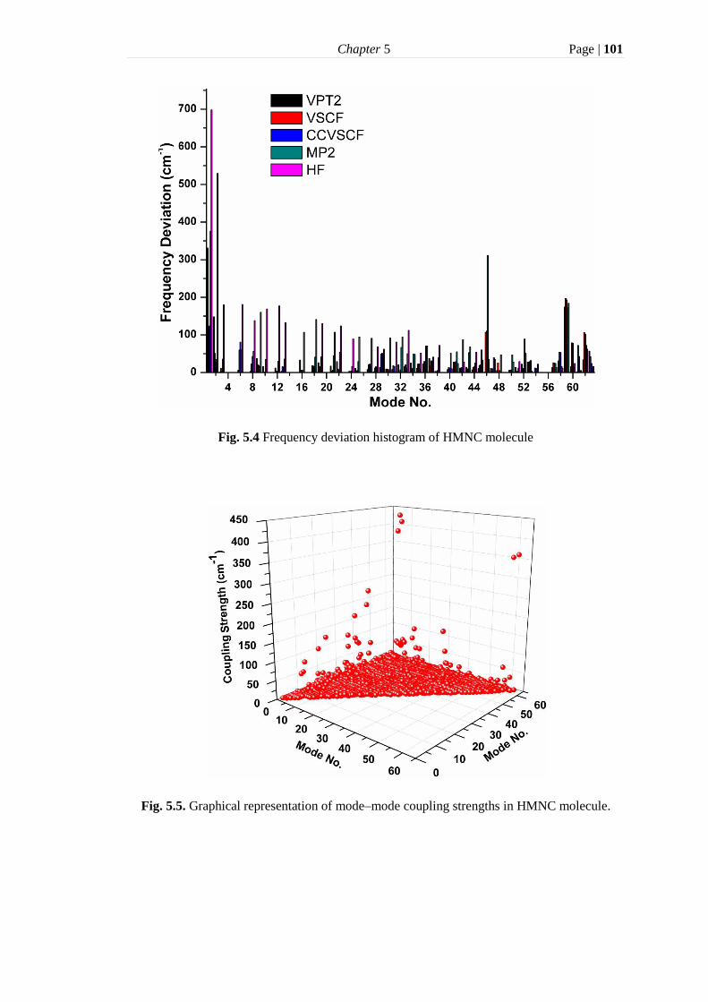
Chapter 5 Page | 101

Fig. 5.4 Frequency deviation histogram of HMNC molecule

Fig. 5.5. Graphical representation of mode–mode coupling strengths in HMNC molecule.

Chapter 5 Page | 102

Fig. 5.6 2D graphical representation of anharmonic mode–mode coupling strengths in HMNC

molecule

Fig. 5.7 Mode–mode coupling strengths between some important modes of HMNC molecule.

Chapter 5 Page | 103

COOH vibrations

The presence of strong intermolecular hydrogen bonding interactions among

carboxylic acid groups lead to a broad band due to O‒H stretching vibrations and a

strong band due to C=O stretching vibrations. In the hydrogen bonded dimers, the

O‒H stretching band of COOH group centres around 3000 cm–1

in IR spectrum and is

superimposed on C‒H stretching bands [37,38]. In the present study, O‒H stretching

vibrations are assigned to modes 1 and 2. Mode 2 is observed in FTIR spectrum at

3195 cm–1

, while mode 1 is observed at 3249 cm–1

. According to PED values, these

modes are pure stretching vibrations. The VPT2 frequencies of modes 1 and 2 are

deviated from the experimental frequencies. These deviations may be due to the

presence of intermolecular (O15‒H23···O37) and intra–molecular (O1‒H16···O14)

hydrogen bonding respectively. The O–H stretching modes show significant

anharmonic corrections in CC–VSCF level of theory. Mode 1 is also strongly coupled

to modes 47, 40, 20 and 42 while mode 2 is coupled to modes 47, 23, 40 and 48 (Fig.

5.7). The strong coupling may also lead to the deviations between observed and

simulated O‒H stretching frequencies in HMNC. The O‒H stretching vibration (mode

1) in the dimer molecule is assigned to 3226, 3141 cm–1

. The O‒H in plane and out of

plane bending vibrations, mixed with other vibrations, are also assigned (Table 5.2).

The assignments of these vibrations are in agreement with the literature [39‒42]. The

O1–H16 and O15–H23 bending vibrations are observed in the FTIR spectrum at 853

and 586 cm–1

. These vibrations are assigned to modes 37 and 46 with 64 and 85 %

PED respectively.

The C=O stretching vibrations absorb very strongly in the 1740‒1700 cm–1

region [38]. In the present study, the observed FTIR frequency at 1733 cm–1

and FT–

Raman frequency at 1719 cm–1

are assigned to C=O stretching vibration in mode 9.

The harmonic frequency, 1732 cm–1

, is in agreement with the experimental data. The

C‒O stretching vibrations are mixed with other modes and assigned in the region

1320–1210 cm−1

[43].

CH3 vibrations

The molecule, HMNC, contains one methyl group. Usually CH3 stretching

vibrations are observed in the region, 3010–2880 cm–1

[44]. In the present study, CH3

asymmetric (mode 6) and symmetric (mode 8) vibrations are observed at 2996 and

Chapter 5 Page | 104

2921 cm–1

in the FTIR spectrum and at 2992 and 2929 cm–1

in the FT–Raman

spectrum respectively. These frequencies are respectively close to the VPT2

anharmonic wavenumbers, 2990 and 2924 cm–1

. According to PED, these have 84%

and 85% contributions in modes 6 and 8 respectively. H21–C12–H20 asymmetric

bending in CH3 group is also predicted in mode 7 at 2920 cm–1

using VSCF method.

From Fig. 5.6 and Fig. 5.7, it is evident that modes 6 and 8 are strongly coupled to

mode 61. The symmetric bending frequency (umbrella motion) corresponding to

mode 20 is observed in the FTIR spectrum at 1364 cm–1

with strong intensity. The

predicted anharmonic frequencies for this mode are 1370, 1355 and 1347 cm–1

at

VPT2, VSCF and CC–VSCF levels of theory respectively. The assignment is in

agreement with the literature [44]. The rocking vibration of CH3 group is observed in

FT–Raman spectrum at 1020 cm–1

which corresponds to mode 31. The predicted

frequency at 1012 cm–1

using VPT2 method is in agreement with the observed value.

The asymmetric bending mode in the methyl group has been predicted in modes 14

and 15, which are mixed with other vibrations. It is also evident from Table 5.2 that

CH3 harmonic frequencies are not affected in dimer.

C‒H vibrations

The aromatic C‒H stretching vibrations generally occur with strong to

medium intensity in the region 3080‒3010 cm–1

, which is the characteristic region for

the ready identification of C‒H stretching vibrations [38]. In this region, the bands

are not appreciably affected by the nature of substituents. The C–H stretching modes

usually appear with strong Raman intensity and are highly polarized. In the present

study, the C‒H stretching vibrations are assigned to modes 3, 4 and 5. The

anharmonic wavenumbers for these modes are predicted by the VPT2 theory at 3072,

3030 and 3029 cm–1

respectively. The FTIR and FT–Raman bands for mode 3 are

observed at 3073 cm–1

and 3074 cm–1

respectively, showing excellent agreement to

anharmonic calculations. However, the C‒H stretching vibrations can posit

anharmonicity as large as 10% [45]. The C–H in–plane bending vibrations usually

occur in the region 1300–1000 cm–1

, whereas, the C–H out of plane bending

vibrations are found in the region 1000–750 cm–1

[46,47].

The in plane C‒H

vibrations are attributed to modes 27 and 28, while, out of plane C‒H deformations

Chapter 5 Page | 105

are assigned to modes 32, 33, 36. These modes are mixed with the other vibrations.

The assignments are also in agreement with the literature [38,48].

Ring vibrations

In HMNC molecule, the ring vibrations are complicate combinations of C=C

and C‒C and C–N vibrations. Generally, C=C and C‒C stretching vibrations in

aromatic compounds are observed in the region 1430‒1650 cm–1

[49] and 1590‒1430

cm–1

[50] respectively. For HMNC, the C9=C10 stretching vibration is assigned to

mode 11. The assignments for C‒C, C=N and C‒N vibrations are also presented in

Table 5.2. The ring breathing and butterfly vibrations have been allocated to modes

41 and 58 respectively. These modes are, respectively, observed at 745 and 218 cm–1

in the FT–Raman spectrum. Other ring vibration modes show a mixed profile.

5.4.3 UV–Vis and HOMO–LUMO analysis

TD–DFT is the most widely used method to calculate the electronic spectra of

molecules. The ground state electronic structure of the molecules is obtained from the

wavefunction of the electron moving within molecule, because molecular orbital can

be treated as electron channels [51]. The experimental and simulated electronic

spectra of HMNC are shown in Fig. 5.8. The vertical excitation energies, absorption

wavelengths and oscillator strengths (f), along with assignments are given in Table

5.3. The major contributions of the transitions were designated using GaussSum

program [52]. TD–DFT calculations have predicted three intense electronic

absorptions at 295, 278 and 246 nm. The oscillator strengths of these transitions in

ethanol are 0.0285, 0.0441 and 0.0023 respectively. The major contributions of these

absorptions correspond to H→L (74%), H–2→L (45%) and H–3→L+1 (92%)

electronic excitations respectively. The corresponding observed transitions are 324,

255 and 207 nm in ethanol and 324, 256 and 206 nm in water.

Frontier molecular orbitals play an important role in studies of optical and

electric properties as well as UV–Vis spectra. HOMO and LUMO energies determine

the ionization potential and electron affinity of the molecule respectively. The

pictorial representation and energies of HOMO and LUMO orbitals of the title

molecule are shown in Fig. 5.9. The red and green colors indicate positive and the

negative phases respectively. The HOMO is spread over entire molecule except the

methyl group, whereas, the LUMO is spread throughout the molecule.

Chapter 5 Page | 106

Fig. 5.8 Experimental and simulated UV-Vis spectra of HMNC molecule.

Table 5.3

Theoretical and experimental UV spectral characteristics of HMNC molecule.

Experimental TDDFT/6–311++G(d,p)

Composition (˃5%) λobs (nm)

Energy (eV)

λcalc (nm)

Oscillator

strength (f)

Energy (eV)

Ethanol water Ethanol water Ethanol water Ethanol water Ethanol water Ethanol Water

301 300 0.0003 0.0003 4.12 4.13 H–1→L (97) H–1→L (96)

324 323 3.78 3.80 295 295 0.0285 0.0278 4.20 4.21

H→L (74)

H–2→L (8) H–2→L+1(8)

H→L+1(8)

H→L (74)

H–2→L (8) H–2→L+1(8)

H→L+1(8)

255 256 4.81 4.80 278 278 0.0441 0.0417 4.46 4.47 H–2→L (45) H→L+1(38)

H→L (16)

H–2→L (44) H→L+1(38)

H→L (17)

276 275 0.00 0.00 4.50 4.52 H–1→L+1(92) H–1→L+1(92) 265 264 0.0014 0.0014 4.67 4.69 H–3→L(94) H–3→L(94)

207 206 5.93 5.96 246 246 0.0023 0.0023 5.03 5.04 H–3→L+1 (92) H–3→L+1 (92)

HOMO‒LUMO energy gap (ΔE), which determines the stability and charge

transfer within the molecule, is found to be 5.3579 eV. The density of state (DOS)

spectrum of HMNC is shown in Fig. 5.10. The values of electronegativity, chemical

potential, chemical hardness and chemical softness for HMNC are 4.2654 eV,

‒4.2654 eV, 2.6790 eV and 0.3733(eV)–1

respectively.

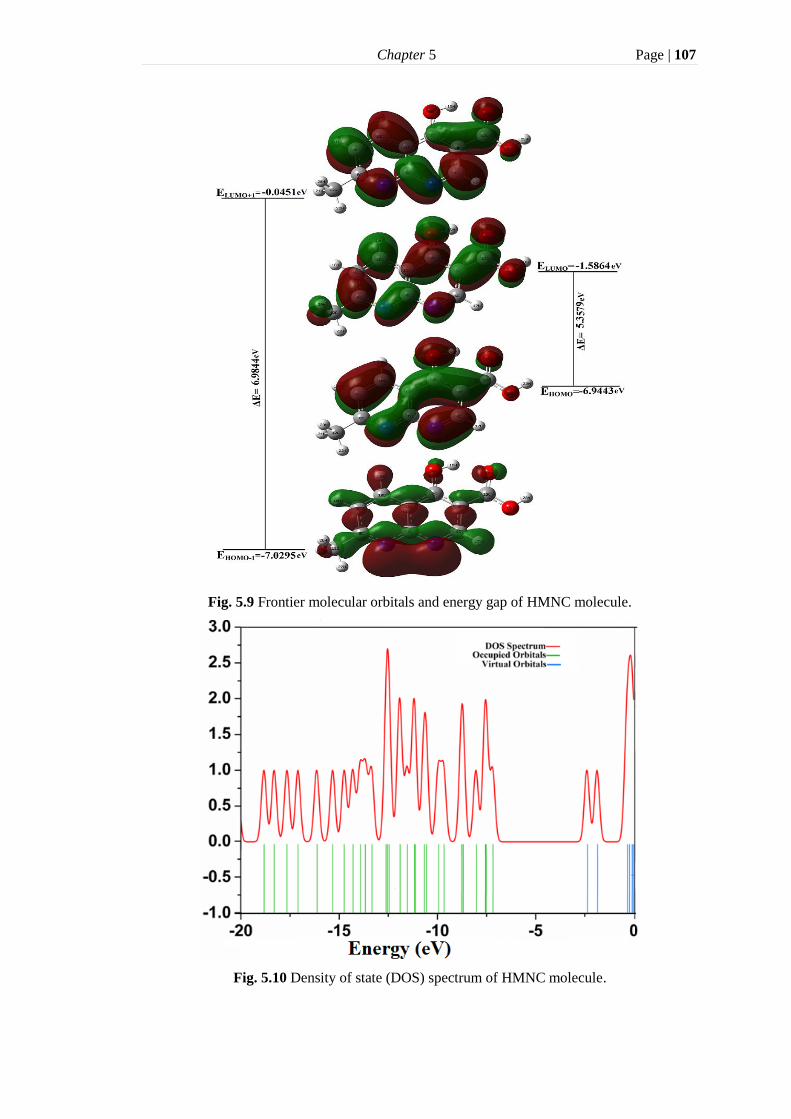
Chapter 5 Page | 107

Fig. 5.9 Frontier molecular orbitals and energy gap of HMNC molecule.

Fig. 5.10 Density of state (DOS) spectrum of HMNC molecule.

Chapter 5 Page | 108

5.4.4 Molecular electrostatic potential

MEP is a real physical property and it expresses the net electrical effect of electrons

and nuclei of a system in the surrounding space. It is used to predict the reactive

behaviour of molecules in both electrophilic and nucleophilic reactions and to study

the biological recognition processes [53,54]. MEP surfaces are obtained by mapping

electrostatic potential onto total electron density with colour code. Red and blue

colours represent electron rich and electron deficient regions respectively. The MEP

map of HMNC with colour range from ‒7.004e–2

(deepest red) to 7.004e–2

(deepest

blue) is shown in Fig. 5.11. It is seen that the negative potential regions correspond to

nitrogen atoms, while the region having the positive potential is spread over H23.

Therefore, N5 and N7 are susceptible to an electrophilic attack, whereas, H23 favours

the nucleophilic attack. The molecular reactive sites are helpful in predicting the

interaction of drugs with proteins.

Fig. 5.11 Molecular electrostatic potential map of HMNC molecule.

5.4.5 Natural bond orbital analysis

The various second order interactions and hyperconjugations in the title molecule are

studied using DFT/6–311G(d,p) level of theory. The hyperconjugative interaction

energy can be deduced from the second order perturbation approach as described in

equation (3.2) of chapter 3. The hybridization of filled orbitals and the second order

Chapter 5 Page | 109

perturbation energy values corresponding to the interactions in HMNC are presented

in Table 5.4 and 5.5 respectively. The highest hyperconjugative interaction energy,

82.92 kcal/mol, is obtained from the (LP1C11)→π*(C2‒C3) interaction. The

hyperconjugative interactions of the lone pair orbitals of C11, O15, O14 and O1 with

antibonding orbitals of C9–C10, C13–O14, C13–O15 and C2–C3, respectively, lead

to the stabilization energy of 54.77, 49.83, 31.22 and 43.85 kcal/mol. Other prominent

interactions π(C2–C3)→π*(C13–O14) and π(C2–C3)→π*(C4–N5) have moderate

stabilisation energies of 28.49 and 26.01 kcal/mol. The interactions between

n(LP2O14)→π*(O38‒H46) and n(LP2O37)→π*(O15‒H23) support the formation of

intermolecular hydrogen bonding in the title molecule. These interactions lead to the

stabilisation energy of 15.53 kcal/mol. The intramolecular interactions between

n(LP1O14)→σ*(O1‒H46) and n(LP2O14)→σ*(O1‒H46) have the stabilisation

energy of 2.22 and 9.71 kcal/mol.

Table 5.4 NBO analysis of HMNC at DFT/6–311G(d,p) level of theory.

Bond (A–B) Occupancy EDA% EDB% NBO (% p character)

σ (O1–C2) 1.99327 66.85 33.15 0.8175sp1.70(62.97)O+ 0.5758sp2.86(73.97)C

σ (O1–H16) 1.9875 76.55 23.45 0.8749sp3.04 (75.20)O+ 0.4843sp0.00(0.19)H

σ (C2–C3) 1.97234 49.46 50.54 0.7033sp1.62(61.75)C+ 0.7109sp1.90(65.44)C

π (C2–C3) 1.66584 38.48 61.52 0.6203sp1.00(99.93)C+ 0.7843p1.00(99.99)C

σ (C2–C11) 1.96770 49.45 50.55 0.7.32sp1.80(64.31)C+ 0.7110sp2.05(67.17)C

σ (C3–C4) 1.97461 52.68 47.32 0.7258sp1.90 (65.45)C+ 0.6879sp1.67(62.54)C

σ (C3–C13) 1.97415 52.01 47.99 0.7212sp2.23(69.04)C+ 0.6927sp1.53(60.51)C

σ (C4–N5) 1.98619 40.93 59.07 0.6398sp1.94(65.90)C+ 0.7686sp1.62(61.70)N

π (C4–N5) 1.80641 39.70 60.30 0.6301sp1.00(99.81)C+ 0.7765sp1.00(99.84)N

σ (C4–H17) 1.97822 60.09 39.91 0.7752sp2.50 (71.42)C+ 0.6318sp0.00(0.05)H

σ (N5–C6) 1.98150 58.44 41.56 0.7645sp1.94(65.94)N+ 0.6447sp2.27(69.40)C

σ (C6–N7) 1.98030 41.10 58.90 0.6411sp2.25(69.18)c+ 0.7647sp1.90(65.42)N

σ (C6–C11) 1.97335 48.08 51.92 0.6934sp1.61(61.66)C+ 0.7205sp2.00(66.63)C

σ (N7–C8) 1.98461 59.60 40.40 0.7720sp1.54(60.65)N+ 0.6356sp2.09(67.63)C

π (N7–C8) 1.76801 60.07 39.93 0.7750sp1.00(99.84)N+ 0.6319sp1.67(99.82)C

σ (C8–C9) 1.97909 49.39 50.61 0.7028sp1.76(63.68)C+ 0.7114sp1.91(65.60)C

σ (C8–C12) 1.97830 50.33 49.67 0.709 sp2.19(68.65)C+ 0.7047sp2.30(69.67)C

σ (C9–C10) 1.97707 49.80 50.20 0.7057sp1.75(63.12)C+ 0.7085sp1.69(62.74)C

π (C9–C10) 1.73965 52.97 47.03 0.7278sp1.00(99.95)C+ 0.6858sp1.00(93.93)C

σ (C9–H18) 1.97872 60.49 39.51 0.7777sp2.48(71.20)C+ 0.6286sp0.00 (0.05)H

σ (C10–C11) 1.96966 48.43 51.57 0.6959sp1.93(65.80)C+ 0.7181sp1.95(66.13)C

σ (C10–H19) 1.97913 61.14 38.86 0.7819sp2.50(71.37)C+ 0.6234sp0.00(0.05)H

σ (C12–H20) 1.97507 60.19 39.81 0.7758sp3.38(77.11)C+ 0.6310sp0.00(0.04)H

σ (C12–H21) 1.97508 60.19 39.81 0.7758sp3.38(77.11)C+ 0.6310sp0.00(0.04)H

σ (C12–H22) 1.98901 61.11 38.89 0.7817sp3.15(75.84)C+ 0.6237sp0.00(0.03)H

σ (C13–O14) 1.99454 34.50 65.50 0.5874sp2.02(66.85)C+ 0.8039sp1.35(57.42)O

π (C13–O14) 1.98678 27.95 72.05 0.5287sp1.00(99.42)C+ 0.8488sp1.00(99.98)O

σ (C13–O15) 1.99492 31.83 68.17 0.5642sp2.64(72.40)C+ 0.8256sp1.74(63.49)O

σ (O15–H23) 1.98666 74.62 25.38 0.8638sp3.48(77.62)O+ 0.5.38sp0.00(0.15)O

LP1O1 1.97265 sp1.161(61.65)

LP2O1 1.80299 sp1.00(99.94)

LP1N5 1.90646 sp2.59(72.10)

LP1C6 0.91055 sp1.00(100)

LP1N7 1.90747 sp2.81 (73.70)

LP2C11 1.07312 sp1.00(100)

LP1O14 1.97129 sp0.75(42.78)

LP2O14 1.84601 sp99.99(99.61)

LP1O15 1.97604 sp1.42(58.70)

LP2O15 1.81462 sp1.00(99.93)

Abbreviation used: ED–Electron density

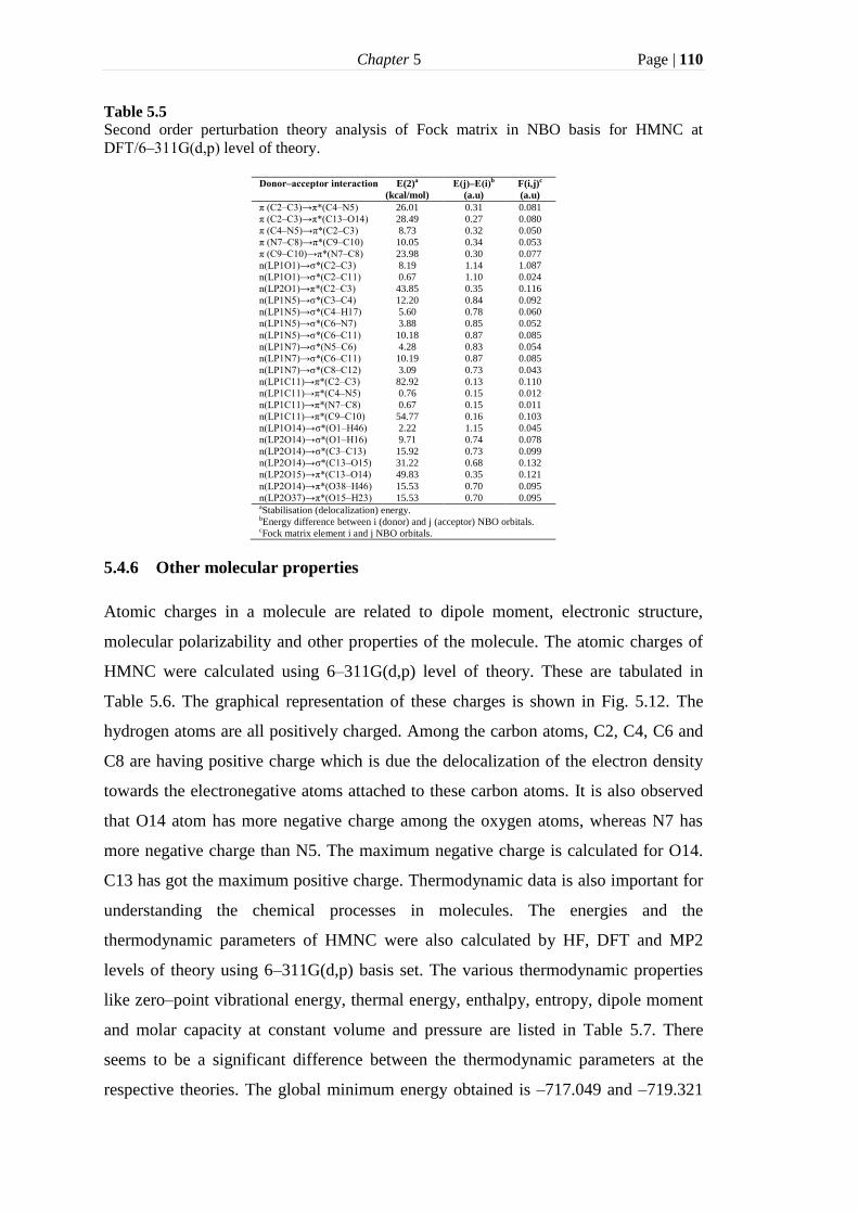
Chapter 5 Page | 110

Table 5.5 Second order perturbation theory analysis of Fock matrix in NBO basis for HMNC at

DFT/6‒311G(d,p) level of theory.

Donor‒acceptor interaction E(2)a

(kcal/mol)

E(j)‒E(i)b

(a.u)

F(i,j)c

(a.u)

π (C2‒C3)→π*(C4‒N5) 26.01 0.31 0.081

π (C2‒C3)→π*(C13‒O14) 28.49 0.27 0.080

π (C4‒N5)→π*(C2‒C3) 8.73 0.32 0.050

π (N7‒C8)→π*(C9‒C10) 10.05 0.34 0.053

π (C9‒C10)→π*(N7‒C8) 23.98 0.30 0.077

n(LP1O1)→σ*(C2‒C3) 8.19 1.14 1.087

n(LP1O1)→σ*(C2‒C11) 0.67 1.10 0.024

n(LP2O1)→π*(C2‒C3) 43.85 0.35 0.116

n(LP1N5)→σ*(C3‒C4) 12.20 0.84 0.092

n(LP1N5)→σ*(C4‒H17) 5.60 0.78 0.060

n(LP1N5)→σ*(C6‒N7) 3.88 0.85 0.052

n(LP1N5)→σ*(C6‒C11) 10.18 0.87 0.085

n(LP1N7)→σ*(N5‒C6) 4.28 0.83 0.054

n(LP1N7)→σ*(C6‒C11) 10.19 0.87 0.085

n(LP1N7)→σ*(C8‒C12) 3.09 0.73 0.043

n(LP1C11)→π*(C2‒C3) 82.92 0.13 0.110

n(LP1C11)→π*(C4‒N5) 0.76 0.15 0.012

n(LP1C11)→π*(N7‒C8) 0.67 0.15 0.011

n(LP1C11)→π*(C9‒C10) 54.77 0.16 0.103

n(LP1O14)→σ*(O1‒H46) 2.22 1.15 0.045

n(LP2O14)→σ*(O1‒H16) 9.71 0.74 0.078

n(LP2O14)→σ*(C3‒C13) 15.92 0.73 0.099

n(LP2O14)→σ*(C13‒O15) 31.22 0.68 0.132

n(LP2O15)→π*(C13‒O14) 49.83 0.35 0.121

n(LP2O14)→π*(O38‒H46) 15.53 0.70 0.095

n(LP2O37)→π*(O15‒H23) 15.53 0.70 0.095 aStabilisation (delocalization) energy. bEnergy difference between i (donor) and j (acceptor) NBO orbitals. cFock matrix element i and j NBO orbitals.

5.4.6 Other molecular properties

Atomic charges in a molecule are related to dipole moment, electronic structure,

molecular polarizability and other properties of the molecule. The atomic charges of

HMNC were calculated using 6–311G(d,p) level of theory. These are tabulated in

Table 5.6. The graphical representation of these charges is shown in Fig. 5.12. The

hydrogen atoms are all positively charged. Among the carbon atoms, C2, C4, C6 and

C8 are having positive charge which is due the delocalization of the electron density

towards the electronegative atoms attached to these carbon atoms. It is also observed

that O14 atom has more negative charge among the oxygen atoms, whereas N7 has

more negative charge than N5. The maximum negative charge is calculated for O14.

C13 has got the maximum positive charge. Thermodynamic data is also important for

understanding the chemical processes in molecules. The energies and the

thermodynamic parameters of HMNC were also calculated by HF, DFT and MP2

levels of theory using 6–311G(d,p) basis set. The various thermodynamic properties

like zero–point vibrational energy, thermal energy, enthalpy, entropy, dipole moment

and molar capacity at constant volume and pressure are listed in Table 5.7. There

seems to be a significant difference between the thermodynamic parameters at the

respective theories. The global minimum energy obtained is ‒717.049 and –719.321

Chapter 5 Page | 111

and ‒721.286 a.u at HF, MP2 and DFT levels of theory respectively. Zero point

vibrational energy is found maximum at HF level and minimum at DFT level. Molar

heat capacities are found in the decreasing order (MP2 > B3LYP > HF). The highest

dipole moment, 2.2780 Debye is calculated by HF, 2.2747 Debye by DFT and 2.4724

Debye by MP2 method. The greater the dipole moment, the stronger is the

intermolecular interaction.

Table 5.6

Natural and Mulliken atomic charges of HMNC using 6–311G(d,p) basis set.

Atom

Natural charge Mulliken Charge

HF

MP2

DFT

HF

MP2

DFT

Isolated Dimer Isolated Dimer

O1 –0.722 –0.733 –0.648 –0.654 –0.445 –0.460 –0.321 –0.335

C2 0.581 0.588 0.449 0.459 0.529 0.526 0.360 0.365

C3 –0.418 –0.427 –0.312 –0.312 –0.517 –0.502 –0.380 –0.369 C4 0.243 0.242 0.137 0.141 0.240 0.235 0.142 0.145

N5 –0.546 –0.549 –0.456 –0.459 –0.426 –0.433 –0.278 –0.285

C6 0.516 0.521 0.414 0.423 0.458 0.448 0.292 0.294 N7 –0.552 –0.553 –0.463 –0.465 –0.442 –0.450 –0.290 –0.299

C8 0.363 0.357 0.282 0.280 0.179 0.177 0.095 0.097

C9 –0.290 –0.296 –0.245 –0.245 –0.202 –0.204 –0.147 –0.145 C10 –0.052 –0.046 –0.120 –0.118 0.132 0.125 0.099 0.094

C11 –0.260 –0.266 –0.176 –0.181 –0.351 –0.329 –0.298 –0.279

C12 –0.533 –0.537 –0.600 –0.604 –0.219 –0.223 –0.272 –0.274 C13 0.986 1.000 0.815 0.845 0.709 0.720 0.469 0.527

O14 –0.752 –0.764 –0.648 –0.732 –0.533 –0.549 –0.392 –0.520

O15 –0.735 –0.739 –0.665 –0.667 –0.416 –0.425 –0.308 –0.326 H16 0.522 0.526 0.500 0.503 0.310 0.318 0.266 0.278

H17 0.180 0.187 0.191 0.198 0.134 0.142 0.123 0.131

H18 0.196 0.199 0.206 0.209 0.101 0.105 0.096 0.100

H19 0.208 0.214 0.219 0.222 0.124 0.132 0.108 0.113

H20 0.185 0.188 0.208 0.211 0.110 0.112 0.122 0.124

H21 0.185 0.188 0.208 0.211 0.110 0.112 0.122 0.124 H22 0.201 0.204 0.221 0.224 0.131 0.134 0.133 0.136

H23 0.494 0.496 0.483 0.510 0.284 0.287 0.258 0.302

Fig. 5.12 Comparison of the natural and Mulliken charges of HMNC molecule.

Chapter 5 Page | 112

Table 5.7 Theoretical computed zero point vibrational energy (kcal mol

–1), thermal energy (kcal mol

–1),

molar heat capacity at constant volume and pressure (cal mol–1

K–1

), Global minimum energy

(a.u), entropy (cal mol–1

K–1

), enthalpy (kcal mol–1

) and dipole moment (Debye) of HMNC at

STP.

Parameters

6-311G(d,p)

HF MP2 B3LYP

Zero–point vibrational energy 115.444 107.166 107.089

Thermal energy 122.542 114.986 114.623

Dipole moment 2.2780 2.4724 2.2747

Global minimum energy (a.u) –717.049 -719.321 –721.286

Molar heat capacity at constant volume (Cv) 43.426 47.736 46.414

Molar heat capacity at constant volume (Cp) 45.413 49.72 48.401

Enthalpy 123.134 115.57 115.215

Entropy 105.879 111.099 108.796

Table 5.8

Calculated components of polarizability (a.u.) and first order hyperpolarizability (a.u.), mean

polarizability ‹ α › (a.u.), anisotropy of the polarizability γ (a.u.) and the mean first order

hyperpolarizability β0 (esu, 1 a.u.=8.639 x 10–33

esu) of HMNC.

B3LYP/6-311G(d,p)

αxx

223.921 βxxx

854.191

αxy

–8.352 βxxy

104.535

αyy

129.707 βxyy

–181.622

αxz

0.000 βyyy

–18.471

αyz

0.000 βxxz

–0.004

αzz

58.239 βxyz

0.000

‹ α › 137.289 βyyz

–0.004

γ 144.660 βxzz

–47.462

βyzz

12.851

βzzz

0.006

β0 (esu) 5.46 x 10

–30

The NLO properties of HMNC computed using DFT level of theory are shown in

Table 5.8. The values of ‹ α › is 137.289 a.u. The computed value of β0 is 5.46×10-30

esu (1a.u.=8.6393 x 10−33

esu) which is 14.6 times more than that of urea. The higher

value of hyperpolazibility reflects the non-linear property of the molecule. However,

to reach that state many other important things like stability, crystal packing and

morphology also come into play.

5.5 Conclusions

In the present study, the anharmonic vibrational spectra of HMNC molecule have

been calculated using HF, DFT and MP2 methods with 6–311G(d,p) level of theory.

The vibrational bands observed in FTIR and FT–Raman spectra are supported by

Chapter 5 Page | 113

calculated anharmonic frequencies at VPT2 (HF, DFT, MP2), VSCF and CC–VSCF

levels of theory and the literature. The VSCF and the CC–VSCF methods based on

2MR–QFF have yielded better results, as indicated by RMS value. VSCF and VPT2

methods respectively show less percentage errors in the regions above and below 900

cm–1

. The deviations between the O–H stretching vibrations of COOH group are

found due to strong coupling and inter and intramolecular hydrogen bonding

interactions. The calculated and experimental electronic spectra in water and ethanol

solvents are in agreement with each other. The hyperpolarizability of HMNC is found

14.6 times more than urea. The negative and the positive potential sites around

nitrogen atoms and H23 atom respectively are observed in MEP mapping.

Chapter 5 Page | 114

References

[1]. S. Massari, D. Daelemans, M.L. Barreca, A. Knezevich, S. Sabatini, V.

Cecchetti, A. Marcello, C. Pannecouque, O. Tabarrini, J. Med. Chem. 53

(2010) 641–648.

[2]. A.A. Fadda, A.M. El–Defrawy, S.A. El–Hadidy, Am. J. Org. Chem. 4 (2012)

87–96.

[3]. G. Roma, G. Grossi, M.D. Braccio, D. Piras, V. Ballabeni, M. Tognolini, S.

Bertoni, E. Baraocelli, Eur. J. Med. Chem. 43 (2008) 1665–1680.

[4]. S. Olepu, P. K. Suryadevara, K. Rivas, K. Yokoyama, C.L.M.J. Verlinde, D.

Chakarbarti, W.C.V. Voorhis, M.H. Gelb, Bioorg. Med. Chem. Lett. 18

(2008) 494–497.

[5]. M.M. Kabanda, E.E. Ebenso, Mol. Simulat. 40 (2014) 1131‒1146.

[6]. J. M. Quintela, C. Peinador, L. Gonzalez, R. Iglesias, A. Parama, F. Alvarez,

M.N. Sanmartin, R. Riguera, Eur. J. Med. Chem. 38 (2003) 265–275.

[7]. T. Aboul–Fadl, F. A. S. Bin–Jubair, O. Aboul–Wafa, Eur. J. Med. Chem. 45

(2010) 4578–4586.

[8]. P. L. Ferrarini, C. Mori, M. Badawneh, F. Franconi, C. Manera, M. Miceli,

G. Saccomanni, Farmaco 55 (2000) 603–610.

[9]. M. Badawneh, C. Manera, C. Mori, G. Saccomanni, P.L. Ferrarini, Farmaco,

57 (2002) 631‒639.

[10]. M. Badawneh, L. Bellini, T. Cavallini, J.A. Jamal, C. Manera, G.

Saccomanni, P.L. Ferrarini, Farmaco, 58 (2003) 859–866.

[11]. E.A. Mohamed, R.M. Abdel–Rahman, Z. El–Gendy, M.M. Ismail, Commun.

Fac. Sci. Univ. Ank. B 40 (1994) 1‒12.

[12]. A.L. Gavrilova, B. Bosnich, Chem. Rev. 104 (2004) 349‒383.

[13]. S. Goswami, R. Mukherjee, Tetrahedron Lett. 38 (1997) 1619‒1622.

[14]. C. Hoock, J. Reichert, J. M. Schmidtke, Molecules 4 (1999) 264–271.

[15]. K. Nakatani, S. Sando, H. Kumasawa, J. Kikuchi, I. Saito, J. Am. Chem.

Soc. 123 (2001) 12650–12657.

[16]. V. Barone, J. Chem. Phys. 122 (2005) 14108–14118.

[17]. R.B. Gerber, M.A. Ratner, Chem. Phys. Lett. 68 (1979) 195–198.

[18]. J.O. Jung, R.B. Gerber, J. Chem. Phys. 105 (1996) 10332–10349.

Chapter 5 Page | 115

[19]. L.S. Norris, M.A. Ratner, A.E. Roitberg, R.B. Gerber, J. Chem. Phys. 105

(1996) 11261–11267.

[20]. M.J. Alam, S. Ahmad, Spectrochim. Acta A 128 (2014) 653–664.

[21]. L. Pele, R.B. Gerber, J. Chem. Phys. 128 (2008) 165105–165110.

[22]. T. Rasheed, S. Ahmad, Vib. Spectrosc. 56 (2011) 51–59.

[23]. R. Gerber, M. Ratner, Adv. Chem. Phys. 70 (1988) 97–132.

[24]. A.D. Becke, Phys. Rev. A 38 (1988) 3098–3100.

[25]. A.D. Becke, J. Chem. Phys. 98 (1993) 5648–5652.

[26]. B.G. Johnson, M.J. Frisch, Chem. Phys. Lett. 216 (1993) 133–140.

[27]. C. Lee, W. Yang, R.G. Parr, Phys. Rev. B 37 (1988) 785–789.

[28]. M.J. Frisch, G.W. Trucks, H.B. Schlegel, G.E. Scuseria, M.A. Robb, J.R.

Cheeseman, et.al., Gaussian 09, Revision D.01, Gaussian, Inc., Wallingford CT,

2009.

[29]. M.W. Schmidt, K.K. Baldridge, J.A. Boatz, S.T. Elbert, M.S. Gordon, et. al.,

J. Comput. Chem. 14 (1993) 1347–1363.

[30]. M.H. Jamroz, Vibrational Energy Distribution Analysis VEDA 4, Warsaw,

2004.

[31]. K. Yagi, K. Hirao, T. Taketsugu, M.W. Schmidt, M.S. Gordon, J. Chem.

Phys. 121 (2004) 1383–1389.

[32]. P. Seidler, T. Kaga, K. Yagi, O. Christiansen, K. Hirao, Chem. Phys. Lett.

483 (2009) 138–142.

[33]. E. D. Glendening, A. E. Reed, J. E. Carpenter, F. Weinhold, NBO Version

3.1.

[34]. A. Achari, S. Neidle, Acta Cryst. B 32 (1976) 600‒602.

[35]. A. Clearfield, M.J. Sims, P. Singh, Acta Cryst. B 28 (1972) 350‒355.

[36]. K. Sasvari, Acta Cryst. B 28 (1972) 2405‒2416.

[37]. N.B. Colthup, L.H. Daly, S.E. Wiberly, Introduction to Infrared and Raman

Spectroscopy, Academic Press, New York, 1990.

[38]. G. Socrates, Infrared and Raman Characteristic Group Frequencies, Third ed.

Wiley Interscience Publications, New York, 1980.

[39]. J. Coates, Interpretation of Infrared spectra, A practical Approach, R.A.

Meyers Ed. John Wiley and Sons Ltd., Chichester, 2000.

[40]. S. Chandra, H. Saleem, N. Sundaraganesan, S. Sebastian, Spectrochim. Acta

A 74 (2009) 704‒713.

Chapter 5 Page | 116

[41]. S. Sebastian, N. Sundaraganesan, S. Manoharan, Spectrochim. Acta A 74

(2009) 312–323.

[42]. V. Arjunan, T. Rani, L. Varalakshmy, S. Mohan, F. Tedlamelekot,

Spectrochim. Acta A 78 (2011) 1449–1454.

[43]. D. Avci, Y. Atalay, M. Sekerci, M. Dincer, Spectrochim. Acta A 73 (2009)

212–217.

[44]. Kucharska, J. Michalski, W. Sasiadek, Z. Talik, I. Bryndal, J. Hanuza,

Spectrochim. Acta A 107 (2013) 317‒325.

[45]. T.K. Roy, R.B. Gerber, Phys. Chem. Chem. Phys. 15 (2013) 9468–9492.

[46]. G. Thilagavathi, M. Arivazhagan, Spectrochim. Acta A 79 (2010) 389–395.

[47]. S. Sebastian, S. Sylvestre, N. Sundaraganesan, M. Amalanathan, S. Ayyapan,

K. Oudayakumar, B. Karthikeyan, Spectrochim. Acta 107 (2013) 167–178.

[48]. M.M. El–Nahass, M.A. Kamel, A.A. El–Barbary, M.A.M. El–Mansy, M.

Ibrahim, Spectrochim. Acta A 111 (2013) 37‒41.

[49]. V. Krishnakumar, N. Surumbarkuzhali, S. Muthunatesan, Spectrochim. Acta

A 71 (2009) 1810–1813.

[50]. D. Shoba, S. Periandy, M. Karabacak, S. Ramalingam, Spectrochim. Acta A

83 (2011) 540‒552.

[51]. T. Yesilkayanak, G. Bimzer, F. Mehmet Emen, U. Florke, N. Kulcu, H.

Arslan, Eur. J. Chem. 1 (2010) 1‒5.

[52]. N.M. O’Boyle, A.L. Tenderholt, K.M. Langner, J. Comput. Chem. 29 (2008)

839‒845.

[53]. I. Fleming, Frontier Orbitals and Organic Chemical Reactions, John Wiley

and Sons, New York, 1976.

[54]. J.S. Murray, K. Sen, Molecular Electrostatic Potentials, Concepts and

Applications, Elsevier, Amesterdam, 1996.

6 Vibrational and electronic spectral analysis of 2,3-

pyrazinedicarboxylic acid

6.1 Introduction

Pyrazine and its derivatives form a class of compounds that are used in

pharmaceutical and flavoring industries [1]. A series of antituberclosis, antifungal,

analeptics and local anesthetics drugs have been synthesized from pyrazine and its

derivatives [2,3]. Pyrazine forms complexes with carboxylic acids and its two

nitrogen atoms are involved in complexation [4]. Owing to significant biological

activities, vibrational studies of pyrazine and its derivatives using both experimental

and theoretical techniques have evinced much interest. The vibrational spectrum of

2,3-dimethylpyrazine [5], 2,5-pyrazinedicarboxylic acid [6], substituted amide of

pyrazine-2-carboxylic acid [7], hydrazinium salts of pyrazinecarboxylic acids [8] as

well as UV and IR absorption spectra of some pyridinecarboxylic acids [9] have been

reported.

The experimental IR and Raman spectra of 2,3-pyrazinedicarboxylic acid

(PDCA) have been investigated by Marquez et.al [10]. Recently, Beaula et al [11].

have carried out the quantum chemical calculations of the molecule using harmonic

approximation and the usual scaling procedure. However, such approach has no first

principles basis and does not provide any insights into the nature of anharmonic part

of the potential which itself is of great interest. The aim of the present study is to

consider anharmonicity using VPT2, VSCF and CC-VSCF methods in order to attain

accuracy in the calculated spectra and also study the effects of anharmonic coupling

on the vibrational modes of PDCA. The electronic spectral analysis is also carried out

using TD-DFT computations. Certain other molecular properties of PDCA molecule

are also discussed.

Chapter 6 Page | 118

6.2 Experimental details

The pure sample (purity ≥ 98%) of PDCA was obtained from Merck Chemical Co.

and used as such for spectral measurements. The FTIR spectrum was recorded in the

region 4000–400 cm-1

on Bruker Tensor 37 spectrometer using KBr pellet technique.

The FT-Raman spectrum was recorded in the region 4000–50 cm-1

on Bruker RFS 27

spectrometer using 1064 nm line of Nd:YAG laser as excitation wavelength. Both the

spectra were measured with a spectral resolution of 2 cm-1

. The electronic absorption

spectra of PDCA in ethanol, methanol and acetonitrile solutions were collected in the

region 800–200 nm, using Lambda-950 UV–Vis–NIR spectrophotometer.

6.3 Computational details

The calculations on PDCA molecule were performed using DFT level of theory

implemented in Gaussian 09 software [12]. The initial geometry of PDCA was

generated from ConQuest 1.14 software database [13]. The geometry was fully

optimized using B3LYP exchange correlation functional with 6-311G(d,p) basis set

under tight convergence criteria. Subsequently, the harmonic and anharmonic

vibrational frequencies along with the intensities were calculated at the same level of

theory. At the optimized geometries, no imaginary frequencies were obtained

implying that the structure is at minimum on the potential energy surface.

Anharmonic corrections in vibrational frequencies were computed using VPT2

approach (implemented in Gaussian 09 package) as well as VSCF, based on 2-mode

coupling representations of the quartic force field (2MR-QFF) and CC-VSCF

methods (implemented in Gamess-US package) [14]. In order to understand the

coupling interactions between mode pairs, the magnitudes of mode-mode coupling for

the ground state were also estimated. In order to understand the effect of

intermolecular interactions on the vibrational spectra, harmonic frequencies of the

PDCA dimer and trimer were also computed using DFT/6-311G(d,p) level of theory.

The vibrational assignments were made on the basis of PED calculations using VEDA

4 program [15] and visual inspection of the atomic displacements. The electronic

absorption spectra were predicted by polarizable continuum model (PCM) using the

integral equation formalism variant (IEFPCM) [16] and the conductor-like polarizable

continuum model (CPCM) [17] in ethanol, methanol and acetonitrile solvents by TD-

Chapter 6 Page | 119

DFT/6-311G(d,p) level of theory. HOMO–LUMO, MEP and NBO analysis were also

performed and discussed.

6.4 Results and discussions

6.4.1 Geometric structure

The conformational flexibility of the title molecule was depicted in molecular energy

profiles (Fig. 6.1) with respect to the rotations about the dihedral angle N2–C3–C7–

O5 from 0◦ to 360

◦, using B3LYP/6-311G(d,p) level of theory. As can be seen from

Fig. 6.1, the most stable conformer is obtained for 0◦ and 360

◦ having energy -641.621

Hartree. The optimized geometry of PDCA monomer, which is non-planar having

dipole moment 2.42 Debye, is shown in Fig. 6.2 (a) along with the atom numbering

scheme. The energy of the optimized structure involving O1–H15···O4 intra-

molecular hydrogen bond is shown in Fig. 6.2 (b). The optimized trimer and dimer

structures are also shown in Fig. 6.2 (c) and Fig. 6.2 (d) respectively. The optimized

geometrical parameters are compared with the single crystal XRD data of PDCA

molecule [18] in Table 6.1. It is observed that the calculated parameters are in

agreement with the XRD data. The elongation of O9–H15 bond in dimer and trimer is

due to the intermolecular hydrogen bonding. The results are also in agreement with

the observations reported for dinicotinic acid and dipicolinic acid [19,20]. In general,

a reasonable agreement is observed between the experimental and computed

geometrical parameters. The computed H···N bond distance in the trimer is 1.79 Å,

and it is equal to 1.83 Å in the crystal structure [18]. In the dimer, the O···H

calculated bond length is 1.62 Å

The geometry of the non-planar intramolecularly hydrogen bonded structure

of PDCA was also optimized in the isolated phase using B3LYP/6-311G(d,p) level of

theory. The energy of the optimized structure (Fig. 6.2 (b)) was found –0.002 Hartree

more than the conformer in Fig. 6.2(a) having dipole moment 7.14 Debye. However,

the crystal structure [18] does not show any intra molecular hydrogen bond and the

calculated IR spectra corresponding to intramolecularly hydrogen bonded structure

were also deviated from the observed spectra. Therefore, the analysis corresponding

to this structure (Fig. 6.2(b)) is not discussed further.

Chapter 6 Page | 120

Fig. 6.1. Potential energy surface scan of 2,3-pyrazinedicarboxylic acid.

Fig. 6.2. Optimized geometries of (a) monomer (b) intramolecularly hydrogen bonded

monomer (c) trimer and (d) dimer structures of 2,3-pyrazinedicarboxylic acid.

Chapter 6 Page | 121

Table 6.1 Optimized geometrical parameters of 2,3-pyrazinedicarboxylic acid at DFT/6-311G(d,p) level

of theory.

Bond length(Å) XRDa Monomer Dimer Trimer Bond Angle (0) XRDa Monomer Dimer Trimer

C1–C3 1.39 1.40 1.40 1.40 C3–C1–C4 123.7 124.0 124.0 121.3

C1–C4 1.50 1.51 1.50 1.51 C3–C1–N6 122.2 121.3 121.0 120.4

C1–N6 1.34 1.33 1.35 1.34 C4–C1–N6 114.0 114.6 115.0 118.2

N2–C3 1.34 1.33 1.35 1.34 C3–N2–C12 117.1 117.1 117.9 117.2

N2–C12 1.33 1.33 1.35 1.33 C1–C3–N2 120.4 121.4 120.9 121.6

C3–C7 1.50 1.50 1.48 1.51 C1–C3–N7 122.2 120.0 120.4 123.2

C4–O8 1.18 1.20 1.25 1.21 N2–C3–C7 117.4 118.6 118.6 115.1

C4–O9 1.32 1.34 1.33 1.31 C1–C4–O8 122.3 123.1 121.6 121.8

O5–C7 1.20 1.21 1.24 1.20 C1–C4–O9 112.4 111.6 113.2 111.7

N6–C11 1.32 1.33 1.35 1.33 O8–C4–O9 125.2 125.1 125.1 126.5

C7–O10 1.30 1.34 1.36 1.34 C1–N6–C11 116.2 116.9 117.7 118.3

O9–H15 0.95 0.97 1.01 1.00 C3–C7–O5 122.2 123.0 122.9 123.0

O10–H16 0.94 0.97 0.98 0.97 C3–C7–O10 111.8 113.3 114.1 111.7

C11–C12 1.38 1.39 1.39 1.39 O5–C7–O10 125.7 123.7 123.0 125.2

C11–H13 0.96 1.09 1.08 1.09 C4–O9–H15 105.9 106.9 113.6 112.6

C12–H14 0.99 1.09 1.08 1.09 C7–O10–H16 113.4 106.2 110.2 106.9

O21···H15 1.62 N6–C11–C12 122.6 121.8 121.3 120.6

O8···H23 1.62 N6–C11–H13 118.8 116.9 116.6 116.6

N6···H47 1.83 1.79 C12–C11–H13 118.5 121.3 122.1 122.7

N18···H15 1.83 1.79 N2–C12–C11 121.5 121.5 121.2 121.9

N38···H32 1.83 1.79 N2–C12–H14 119.3 117.2 116.7 117.0

C11–C12–H14 119.2 121.3 122.1 121.1

O21···H15–O9 173.8

O8···H23–O26 174.6

N6···H47–O41 176 175.7

N18···H15–O9 176 176.1

N38···H32–O26 176 176.0

a= Ref. [18]

6.4.2 Vibrational analysis

The molecule, PDCA, consists of 16 atoms and 42 vibrational degrees of freedom. In

order to investigate the spectroscopic signature, vibrational spectra of PDCA

monomer were simulated and compared with the experimental data as shown in Fig.

6.3 and Fig. 6.4 respectively. The calculated harmonic infrared and Raman spectra of

the trimer structure are also plotted in Fig. 6.5. The theoretical IR and Raman spectra

were simulated using Lorentzian line shape with FWHM, 6 cm-1

. The vibrational

modes along with their assignments are presented in Table 6.2. It is observed that the

experimental and simulated anharmonic spectra are well comparable. The RMS

values in Table 6.2 indicate that VSCF computed anharmonic frequencies are in more

Chapter 6 Page | 122

Fig. 6.3 Comparison of the experimental and calculated anharmonic IR spectra of

2,3-pyrazinedicarboxylic acid.

Fig. 6.4. Comparison of the experimental and calculated Raman spectra of

2,3-pyrazinedicarboxylic acid.

Chapter 6 Page | 123

Fig. 6.5. Harmonic IR and Raman spectra of 2,3-pyrazinedicarboxylic acid trimer.

close agreement with the observed data as compared to VPT2 and CC-VSCF

computed anharmonic frequencies. However,VPT2 approach has lesser computational

cost and it is at least an order of magnitude cheaper than VSCF and CC–VSCF

methods. The graphical representations of mode-mode coupling and coupling

strengths of some important mode pairs are also shown in Fig. 6.6 and Fig. 6.7

respectively. The highest coupling strengths (>350 cm-1

) are observed between the

mode pairs (1, 29) and (2, 31). It is also observed that the mode pairs (3, 20), (3, 21),

(4, 20) and (4, 21) have high coupling strengths and involve displacements of the

same atoms. Therefore, it is confirmed that the anharmonic coupling between normal

modes involving displacements of the same atoms are typically stronger. Similar

observations have been also reported earlier [21,22]. The assignments of various

vibrational modes of PDCA are discussed below.

Chapter 6 Page | 124

Table 6.2

Comparison and assignments of the experimental and computed frequencies of 2,3-pyrazinedicarboxylic acid.

M

Experimental B3LYP/6-311G(d,p)

Composition (%)

FTIR

FT-Raman

Har

VPT2

A

R

VSCF

CC-VSCF

Aa

Dimer

Har

Trimer

Har

1 3761 3563 96.1 40.8 3448 3513 87.1 3674 3643 3747 3747 3747 ν OH (100)

2 3265s 3747 3548 80.8 50.5 3429 3471 72.3 3010 2880 3151 3150 3112 ν OH (100)

3 3102vw 3176 3030 29.8 117.8 3025 3004 32.3 3214 3214 3186 3186 3186 ν CH (99) 4 3082vw 3098m 3158 3036 1.0 41.1 2983 2961 1.0 3194 3194 3170 3170 3169 ν CH (100)

2814 1099+1716

2609 1447+1161, 1399+1207 2525 1265×2

5 1754vs 1841 1809 304.6 39.4 1803 1802 294.6 1734 1686 1839 1839 1839 ν C=O (86)

6 1716vs 1724s 1804 1771 267.8 64.6 1767 1766 260.3 1671 1634 1786 1774 1774 ν C=O (87) 7 1577m 1578m 1595 1553 11.1 48.9 1567 1563 10.8 1564 1561 1606 1606 1605 ν [C9-C10 + ν [C7-C8](59) + β HCN(18)

8 1543w 1542s 1581 1542 11.0 102.2 1554 1551 10.9 1554 1555 1581 1581 1581 νasCN (82)

9 1447m 1480 1446 26.4 1.6 1460 1458 6.3 1483 1470 1480 1478 1478 ν CN (37) + β HCN(52) 10 1399m 1454 1414 35.6 42.5 1431 1428 35.8 1467 1446 1470 1468 1468 ν CN (10) + β HCN(24) + β[ C9-C10-N6 + C8-C7-N5] (32) +β OCO(12)

11 1265vs 1262m 1397 1378 88.8 12.1 1377 1373 88.2 1446 1421 1435 1434 1410 β HOC(57) + ν [C7-C11+ C8-C12] (10)

12 1364 1311 57.5 7.8 1351 1346 56.6 1382 1368 1376 1376 1370 β HOC(52) + β HCN(14) 13 1227w 1268 1238 16.2 3.7 1259 1257 15.1 1259 1254 1264 1264 1264 ν CN (33) + ν [C7-C11+ C8-C12] (10) +β HOC(-15) + β HCN(28)

14 1246 1215 32.8 83.6 1242 1236 32.2 1233 1233 1233 ν[ C9-N5 + C10-N6](33) + ν C7-C8 (10) + β H-C(28) + β HOC(15)

15 1207w 1232 1194 16.4 5.2 1217 1213 17.3 1220 1218 1222 1221 1220 νas CN (77) + β H-C (12) 16 1182s 1183w 1197 1159 226.8 17.6 1195 1188 225.0 1203 1210 ν[O1-C11+ O2-C12] (23) + ν CN (19) + β HOC(17) + β HCN (10)

+ β[C7-C11-O1 + C8-C12-O2](11) 17 1161sh 1153 1120 192.6 8.5 1146 1140 190.4 1144 1117 1174 1170 1170 ν [O1-C11+ O2-C12] (54) + β [C9-C10-N6 + C8-C7-N5](12) + β HCN (8)

18 1099vs 1096vw 1093 1071 210.8 4.6 1079 1077 209.3 1113 1107 1107 Ring breathing (73)

19 1066s 1082 1060 6.9 107.3 1072 1068 7.5 1085 1081 1085 1085 1085 Star of David vibration (71) 20 992vw 996vw 1002 977 0.03 0.4 1018 1009 0.1 1008 1009 1015 1014 1013 γ H-C (81) + τ N5-C9-C10-N6 (11)

21 870m 870vw 894 871 13.0 1.4 917 908 12.4 898 898 903 901 902 γ H-C (83)

22 866 853 10.5 22.1 857 856 10.5 872 873 874 874 869 ν [O1-C11+ O2-C12] (10) + ν [C7-C11+ C8-C12] (19) + β [N5-C9-C10 + N6-C10-C9](47)

23 835w 834vw 855 841 10.7 6.7 848 848 10.7 882 880 853 853 852 γ [C11-C8-N5-C7 + C12-C7-N6-C8](82)

24 794m 784s 782 770 69.9 28.0 790 827 70.0 763 761 785 785 785 γ [C11-C8-N5-C7 + C12-C7-N6-C8](10) + γ[O3-C7-O1-C11 + O4-C8-O2-C12](69) 25 766sh 759w 759 743 33.6 4.6 769 766 33.0 754 747 743 741 741 β OCO (15) + ν N-C (32)

26 693w 733 720 28.3 111.4 737 734 28.6 728 724 767 761 761 τ [N5-C9-C10-N6 + N6-C8-C7-N5] (67)

27 678m 662 655 75.6 16.2 667 665 75.1 672 665 687 682 682 β OCO (67) + τ HOCC (9) 28 642vw 640w 634 627 10.6 13.6 636 630 9.8 637 636 647 647 647 β CNC (80)

29 617 602 101.6 59.0 675 571 88.5 634 606 606 606 γ [OH](79)

30 544 vw 601 590 5.1 10.6 613 600 5.4 609 614 598 597 596 γ [OH] (86) 31 593 569 88.3 42.3 664 479 76.7 594 β [C7-C11-O1 + C8-C12-O2](63)

32 537vw 516 514 15.9 17.2 535 514 15.5 534 553 532 529 529 β [O3-C11-C7 + O4-C12-C8] (12) + τ NCCN (35)

Chapter 6 Page | 125

33 425vw 413w 432 423 2.1 13.8 450 438 2.3 450 446 450 439 449 τ [C7-N5-C9-C10 + C10-N6-C8-C7](73)

34 397 391 1.9 75.3 405 400 1.9 383 367 421 421 409 ν CN (-28) + δ OCO (23) + τ NCCN (22) 35 360vw 344 339 6.6 17.3 352 349 6.6 356 356 356 β [O1-C11-C7 + O2-C12-C8] (57) + β [C9-C10-N6+ C10-C9-N5] (10)

36 343m 325 319 1.1 52.1 330 328 1.1 344 340 326 326 325 ν [C7-C11+ O8-C12] (42)

37 213m 236 232 0.8 44.4 254 248 0.9 256 275 269 268 259 β [C12-C8-N6 + C11-C7-N5](71) 38 156s 171 167 3.7 102.9 193 187 3.6 165 143 186 180 179 γ [C11-C8-N5-C7 + C12-C7-N6-C8](62)+γ [O3-C7-O1-C11+ O4-C8-O2-C12](11)

39 145 140 1.4 49.7 159 154 1.4 126 112 175 165 162 β [C11-C7-N5 + C12-C8-N6](57)+ τ[C7-C8-C12-O2 + C8-C7-C11-O1] (17)

40 120vs 99 91 2.1 120.4 114 112 1.9 104 94 104 99 99 γ [C11-C8-N5-C7 + C12-C7-N6-C8](75) 41 82vs 89 84 0.4 137.0 108 105 0.4 70 61 58 57 46 τ [C-COOH] (57)

42 66vs 18 27 1.8 853.4 61 53 1.5 20 15 28 25 24 τ [C-COOH] (95)

RMS 95 59 49 54

Abbreviation used: M-modes, Har- Harmonic wavenumbers, , A-IR intensity (km/mol), R-Raman intensity (arb unit), Aa-anharmonic intensity(km/mol), ν-stretching, νas-asymmetric stretching, β-bending, τ-torsional, γ-out of

plane vibrations, δ-scissoring, w-weak, m-medium, sh-shoulder, s-strong, vs-very strong, vw-very weak

Table 6.2 continued....

Chapter 6 Page | 126

Fig. 6.6. Graphical representation of mode-mode coupling strength in

2,3-pyrazinedicarboxylic acid.

Fig. 6.7. Mode–mode coupling strength between some important mode pairs of 2,3-

pyrazinedicarboxylic acid.

Chapter 6 Page | 127

COOH vibrations

The molecules containing carboxyl groups generally form stable dimers in the

condensed phase. The spectra of carboxylic acid derivatives are best characterized by

the carbonyl and hydroxyl group vibrations. The absorption due to carbonyl group is

important in the infrared spectrum because of its strong intensity of absorption and

high sensitivity to the environment. Being highly polar, carbonyl bond gives strong

absorption bands in the region 1750–1700 cm-1

[23,24]. In the present study, strong

absorption bands observed at 1754 (mode 5) and 1716 cm-1

(mode 6) are due to C=O

stretching vibrations. The PED contributions are more than 85% in these modes. The

calculated anharmonic frequencies overestimate the observed values. However, in the

dimer, the computed frequencies corresponding to mode 5 and 6 are 1734,1686 and

1671,1634 cm-1

respectively. These assignments are also in well agreement with the

literature [25,10]. The modes, 16 and 17 are observed at 1182 and 1161 cm-1

respectively and they have significant contributions from C–O stretching vibrations.

O–H vibrations are characteristics of carboxyl group which generally exhibit a

broad band in the region 3000–2500 cm-1

due to O–H stretching [26]. The pure O–H

stretching vibrations with 100% PED contributions are assigned to modes 1 and 2.

Mode 2 is observed in the FTIR spectrum at 3265 cm-1

, while the band corresponding

to mode 1 is missing in the experimental spectra. The calculated O–H anharmonic

frequencies are largely deviated from the observed frequencies. From Fig. 6.7, it is

observed that these two modes are strongly coupled with modes 29 and 31

respectively, which may lead to the deviation between the simulated and experimental

data. However, mode 2 is computed at 3151,3150,3112 cm-1

in the trimer, which is

close to the experimental value. The O–C=O in-plane bending vibrations are observed

at 766 and 678 cm-1

. The corresponding CC-VSCF anharmonic frequencies are 766

and 665 cm-1

respectively.

C–H vibrations

C–H stretching, in-plane and out-of-plane bending vibrations have been

generally observed in the regions, 3100–3000 cm-1

, 1300–1000 cm

-1 and 1000–750

cm-1

respectively [27,28]. In the present study, C–H stretching frequencies are

assigned to modes 3 and 4. Mode 4 is observed at 3082 cm-1

in the FTIR spectrum and

at 3098 cm-1

in the FT-Raman spectrum, while mode 3 is observed at 3102 cm-1

in the

Chapter 6 Page | 128

FTIR spectrum. The VPT2 computed frequencies for these modes at 3036 and 3030

cm-1

respectively are more close to the experimental data than VSCF and CC-VSCF

computed frequencies. From Fig. 6.7, it is observed that modes 3 and 4 are also

strongly coupled with modes 20 and 21, which leads to the deviation of the calculated

frequencies from the observed values. The strong coupling (>85 cm-1

) involves the C–

H displacements which confirm that coupling strengths between modes involving

same atoms are larger [21,22]. Modes 20 and 21 are assigned to C–H out of plane

vibrations which are observed at 992 and 870 cm-1

respectively. The corresponding

anharmonic frequencies are 977 and 871 cm-1

at VPT2 respectively. The assignments

are also in agreement with 2,3-dimethylpyrazine and 3,5-pyridinedicarboxylic acid

[5,29].

Ring vibrations

The ring vibrations in PDCA molecule are complicate combinations of C–C

and C–N vibrations. The C–N stretching modes are observed in the region 1545–1165

cm-1

in the spectra of PDCA molecule. The calculated frequencies are in close

agreement with experimental frequencies and the literature [10,6]. The C–C

frequencies present mixed profile and are allocated to modes 11, 13 and 14. Besides

C–C and C–N vibrations, ring breathing and Star of David vibrations are also

observed in the title molecule. The ring breathing vibration (mode 18), observed at

1099 cm-1

in the FTIR spectrum and at 1096 cm-1

in the FT-Raman spectrum is in

agreement with the harmonic frequency at 1093 cm-1

. The anharmonic frequencies are

1071, 1079 and 1077 cm-1

at VPT2, VSCF and CC-VSCF levels of theory

respectively. The Star of David vibration is described as the contraction of the ring at

the triangle formed by C7, N6, C9 and an expansion of the ring at the triangle formed

by C8, N5, C10 and vice versa. It is observed at 1066 cm-1

in the FT-Raman

spectrum.

The bands observed in the region 3000–2500 cm-1

of the IR spectrum may be

due to the non-fundamental bands of the pyrazine ring. The broad and less intense

bands observed at 2814, 2609 cm-1

are combination bands while the band observed at

2525 cm-1

is an overtone band. These bands also provide a more unique identification

in PDCA.

Chapter 6 Page | 129

6.4.3 UV-Vis and HOMO–LUMO analysis

The TD-DFT is one of the popular and widely used approaches for the calculations of

excitation energies, oscillator strengths and excited state geometries of medium to

large molecular systems. UV-Vis spectroscopy is frequently used as a strong and

accurate method to describe low-lying excited states of conjugated molecules and has

consequently been applied to solve many physical and chemical problems. The

experimental and computed UV-Vis spectra of PDCA using IEF-PCM and CPCM

models are compared in Fig. 6.8 (A), Fig. 6.8 (B) and Fig. 6.8 (C) respectively. The

calculated spectra in ethanol, methanol and acetonitrile solvents were simulated using

Gaussian band shape with 1500 cm-1

FWHM. The vertical excitation energies,

oscillator strengths (f) and transition wavelengths along with the assignments are

presented in Table 6.3. The nature and contributions of the transitions were identified

by Gauss-sum 2.2 program [30]. The calculated transition wavelengths are same in

both the theoretical models and do not show any considerable solvent effect. These

transitions are observed at 320, 270 and 209 nm in ethanol, 318, 269, and 215 nm in

methanol, and 317, 268 and 211 nm in acetonitrile respectively. The maximum

absorption wavelength, 215 nm corresponds to H-2→L (68%) transition whereas, the

absorptions at 320 and 270 nm are assigned to H→L (96%) and H→L+1 (96%).

Beaula et. al. have reported an absorption at 277 nm in water [11]. The absorption

wavelengths reported for 2,3-pyridinedicarboxylic acid, 2,4-pyridinedicarboxylic

acid, 2,5-pyridine dicarboxylic acid, 2,6-pyridinedicarboxylic acid, 3,4-

pyridinedicarboxylic acid and 3,5 pyridinedicarboxylic acid are also found to be in

good agreement with our results for PDCA [9].

The HOMO, LUMO orbitals and their energy gaps for PDCA were calculated

using B3LYP/6-311G(d,p) level of theory by TD-DFT method and their pictorial

representation is shown in Fig. 6.9. HOMO and LUMO analyses explain the charge

transfer within the molecule. The HOMO has ability to donate electrons, whereas the

LUMO receives electrons [31]. The calculated HOMO–LUMO energy gap is found to

be 4.81 eV. From Fig. 6.9, it can be seen that HOMO and LUMO orbitals are

localized on the whole molecule.

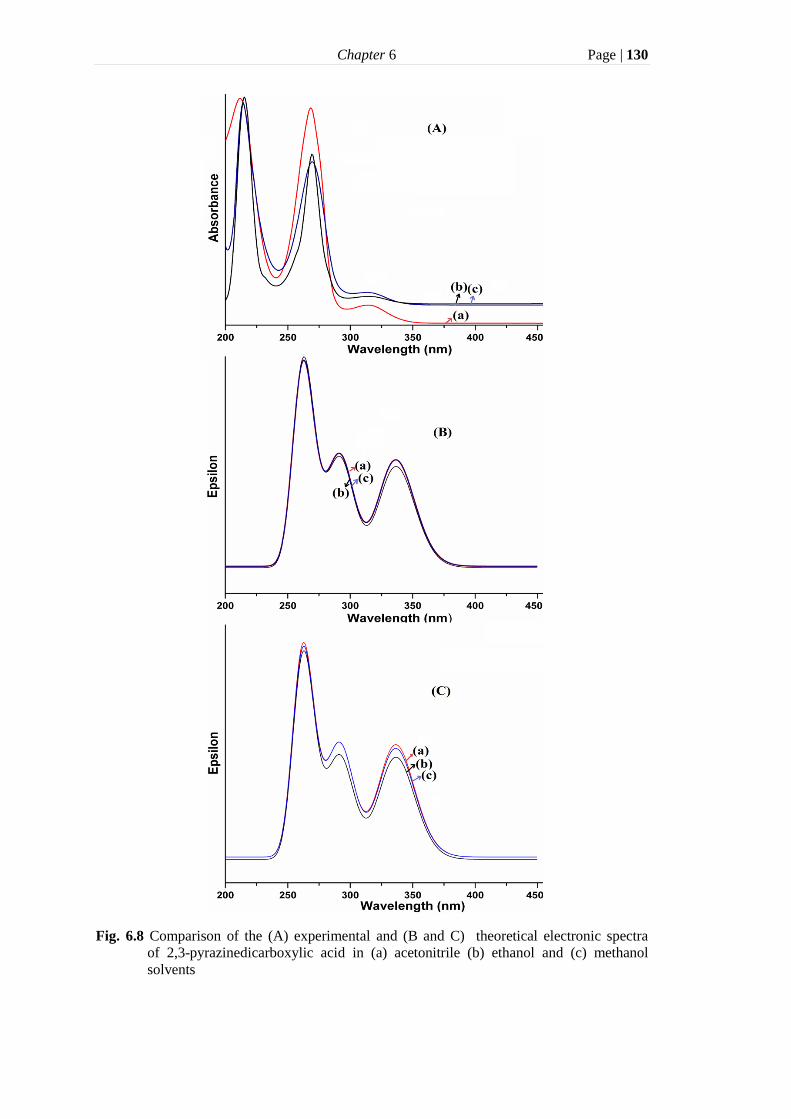
Chapter 6 Page | 130

Fig. 6.8 Comparison of the (A) experimental and (B and C) theoretical electronic spectra

of 2,3-pyrazinedicarboxylic acid in (a) acetonitrile (b) ethanol and (c) methanol

solvents

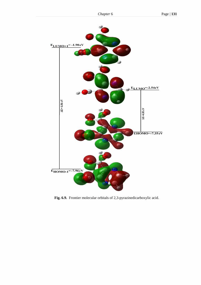
Chapter 6 Page | 131

Fig. 6.9. Frontier molecular orbitals of 2,3-pyrazinedicarboxylic acid.

Chapter 6 Page | 132

Table 6.3

Theoretical and experimental UV spectral characteristics of 2,3-pyrazinedicarboxylic acid.

Experimental

TD-DFT/6-311G(d,p)

IEF-PCM model CPCM model

ethanol methanol acetonitrile ethanol Methanol acetonitrile ethanol methanol acetonitrile

Composition (%) λ E λ E λ E λ f E λ f E λ f E λ f E λ f E λ f E

320 3.83 318 3.86 317 3.87 336 0.0027 3.68 336 0.0027 3.68 336 0.0027 3.68 336 0.003 3.68 336 0.0029 3.68 336 0.003 3.68 (96) H→L

270 4.54 269 4.56 268 4.58 291 0.0029 4.25 291 0.0028 4.25 291 0.0028 4.25 291 0.003 4.25 291 0.003 4.25 291 0.003 4.25 (96) H→L+1

215 5.71 215 5.71 211 5.82 262 0.0056 4.72 262 0.0052 4.72 262 0.0052 4.72 262 0.0061 4.72 262 0.0056 4.72 262 0.0057 4.72 (68) H-2→L

Abbreviation used: λ-excitation wavelength (nm), E-excitation energy (eV), H-Homo, L-Lumo, f-oscillator strength.

Chapter 6 Page | 133

6.4.4 Molecular electrostatic potential

The MEP of PDCA was computed at B3LYP/6-311G(d,p) level and shown in Fig.

6.10 with colour range from –6.209e-2 to 6.209e-2. The red and blue areas refer to the

regions of negative and positive potentials which correspond to the electron rich and

electron poor regions respectively. The green color signifies the neutral electrostatic

potential. It is observed that the most electronegative potential region is over O8 while

the regions around H15 and H16 atoms are more electropositive in PDCA.

Fig. 6.10. Molecular electrostatic potential map of 2,3-pyrazinedicarboxylic acid.

6.4.5 Natural bond orbital analysis

The NBO analysis of PDCA was carried out using DFT/6-311G(d,p) level of theory

using NBO 3.1 program [32]. The hybridization of filled orbital is shown in Table 6.4.

The second order perturbation energy values (E(2)

) corresponding to the important

interactions between the electron donors and acceptors, are presented in Table 6.5.

The strongest interactions from n(LP2O10)→π*(O5‒C7), n(LP2O9)→π*(C4‒O8),

n(LP2O8)→σ*(C4‒O9) and n(LP2O5)→σ*(C7‒O10) yield stabilization energy of

48.29, 45.87, 31.15 and 30.71 kcal/mol. Other interaction energies are also listed in

Chapter 6 Page | 134

Table 6.5. Significant stabilization energies are also obtained in the trimer structure of

the title molecule.

Table 6.4

NBO analysis of 2,3-pyrazinedicarboxylic acid at DFT/6-311G(d,p) level of theory.

Bond (A-B) Occupancy EDA% EDB% NBO (% p character)

σ (C1‒C3) 1.98069 49.87 50.13 0.7062sp1.63(61.89)C+ 0.7080sp1.68(62.64)C

π (C1‒C3) 1.57478 47.38 52.62 0.6883sp99.99(99.94)C+ 0.7254sp1.00(99.98)C

σ (C1‒C4) 1.97304 52.73 47.27 0.7262sp2.27(69.37)C+ 0.6875sp1.74(63.52)C

σ (C1‒N6) 1.98062 41.24 58.76 0.6422sp2.20 (68.70)C+ 0.7666sp1.78(63.93)N

σ (N2‒C3) 1.98366 58.49 41.51 0.7648sp1.80 (64.21)N+ 0.6443sp2.16(68.31)C

σ (N2‒C12) 1.98569 59.72 40.28 0.7728sp1.80 (64.21)N+ 0.6347sp2.13(68.02)C

π (N2‒C12) 1.69550 55.99 44.01 0.7482sp1.00 (99.84)N+ 0.6634sp1.00(99.86)C

σ (C3‒C7) 1.97595 52.24 47.76 0.7228sp2.23 (69.03)C+ 0.6911sp1.65(62.28)H

σ (C4‒O8) 1.99511 34.40 65.60 0.5865sp1.90 (65.42)C+ 0.8100sp1.42(58.65)O

π (C4‒O8) 1.99223 31.05 68.95 0.5572sp99.99 (99.03)C+ 0.8304sp99.99(99.13)O

σ (C4‒O9) 1.99490 31.58 68.42 0.5619sp2.51 (71.31)C+ 0.78272sp1.89(65.32)O

σ (O5‒C7) 1.99564 65.25 34.75 0.8078sp1.44(58.94)O+ 0.5895sp1.93(65.79)C

π (O5‒C7) 1.98086 69.57 30.43 0.83413sp99.99 (99.85)C+ 0.551699.99(99.45)C

σ (N6‒C11) 1.98485 59.67 40.33 0.7725sp1.83 (64.56)N+ 0.6351sp2.13(68.00)C

π (N6‒C11) 1.68602 57.79 42.21 0.7602sp1..00(99.85)N+ 0.6497sp1.00 (99.85)C

σ (C7‒O10) 1.99498 32.00 68.00 0.5657sp2.55 (71.71)C+ 0.8246sp1.93(65.75)O

σ (O9‒H15) 1.98355 74.55 25.45 0.8634sp3.90 (79.53)O+ 0.5045sp0.00(0.17)C

σ (O10‒H16) 1.98515 74.51 25.49 0.8632sp3.90 (79.50)O+ 0.50490.00(0.18)H

σ (C11‒C12) 1.99197 50.03 49.97 0.7073sp1.62(61.78)C+ 0.7069sp1.63(61.92)C

σ (C11‒H13) 1.98099 60.17 39.83 0.7757sp2.34(69.99)C+ 0.6311sp0.00(0.05)H

σ (C12‒H14) 1.98133 60.19 39.81 0.7758sp2.32 (69.83)C+ 0.6310sp0.00(0.05)H

LP1N2 sp2.50 (71.35)

LP1O5 sp0.69(41.00)

LP2O5 sp99.99 (99.98)

LP1N6 sp2.49(71.28)

LP1O8 sp0.73(42.06)

LP2O8 sp99.99(99.84)

LP1O9 sp1.22(54.99)

LP2O9 sp99.99(99.91)

LP1O10 sp1.20(54.55)

LP2O10 sp1.00(99.93)

Abbreviation used: ED-Electron density

Table 6.5

Second order perturbation analysis of Fock matrix of 2,3-pyrazinedicarboxylic acid monomer

and trimer at DFT/6-311G(d,p) level of theory.

Donor-acceptor interaction E(2)a

(kcal/mol)

E(j)-E(i)b

(a.u)

F(i,j)c

(a.u)

n(LP1N2)→σ*(C1‒C3) 10.14 0.89 0.085

n(LP1N2)→σ*(C3‒C7) 3.24 0.74 0.044

n(LP1N2)→σ*(C11‒C12) 8.81 0.89 0.080 n(LP1N2)→σ*(C12‒H14) 4.34 0.78 0.053

n(LP1O5)→ σ*(C8‒C9) 2.53 1.08 0.047

n(LP1O5)→ π*(C4‒O8) 0.57 0.73 0.019

n(LP1O5)→σ*(C7‒O10) 1.11 1.06 0.031

n(LP2O5)→σ*(C3‒C7) 18.87 0.66 0.101

n(LP2O5)→ π*( C4‒O8) 2.44 0.31 0.025

n(LP2O5)→ σ*( C7‒O10) 30.71 0.64 0.127

n(LP1N6)→σ*(C1‒C3) 9.83 0.89 0.084

n(LP1N6)→σ*(C1‒C4) 2.75 0.74 0.040

n(LP1N6)→σ*(C11‒H13) 4.26 0.78 0.052

n(LP1O8)→ σ*(C1‒C4) 2.28 1.06 0.045

n(LP1O8)→ σ*(C4‒O9) 1.91 1.05 0.041

n(LP2O8)→ π*(C1‒C3) 0.79 0.27 0.013

n(LP2O8)→ σ*(C1‒C4) 21.18 0.63 0.106

n(LP2O8)→ σ*(C4‒O9) 31.15 0.63 0.127

Chapter 6 Page | 135

n(LP1O9)→ σ*(C4‒O8) 6.58 1.24 0.081

n(LP2O9)→ π*(C4‒O8) 45.87 0.36 0.115

n(LP1O10)→ σ*(O5‒C7) 6.28 1.23 0.078

n(LP2O10)→ π*(O5‒C7) 48.29 0.34 0.116

Trimer

From Unit 1 to 2

n(LP1O8)→σ*(C28‒H30) 0.11 1.12 0.010 n(LP2O8)→σ*( C27‒C28) 0.08 0.80 0.007

n(LP2O8)→σ*( C28‒H30) 0.31 0.70 0.014

n(LP1O9)→σ*(N18‒C19) 0.06 1.06 0.007 n(LP2O9)→ π*(N18‒C28) 0.06 0.29 0.004

From Unit 1 to 3

n(LP1N6)→σ*(C36‒O41) 0.07 0.80 0.007

n(LP1N6)→σ*( O41‒H47) 23.38 0.78 0.123 n(LP1O9)→σ*( C36‒O41) 0.19 0.98 0.012

n(LP1O9)→σ*( O41‒H47) 0.60 0.96 0.022

From Unit 2 to 1 n(LP1N18)→σ*(C4‒O9) 0.07 0.80 0.007

n(LP1N18)→σ*(O9–H15) 23.67 0.78 0.123

n(LP1O26)→σ*(C4–O9) 0.18 0.98 0.012 n(LP1O26)→σ*(O9–H15) 0.96 0.98 0.021

From Unit 3 to 1

n(LP1O40)→σ*(C11–H13) 0.11 1.12 0.010 n(LP2O40)→σ*(C11–C12) 0.08 0.80 0.007

n(LP2O40)→σ*(C11–H13) 0.31 0.70 0.013

n(LP1O41)→σ*(C1–N6) 0.06 1.06 0.007 n(LP2O41)→ π*(C11–N6) 0.06 0.29 0.004

From Unit 3 to 2

n(LP1N38)→σ*(C23–O26) 0.07 0.80 0.007 n(LP1N38)→σ*(O26–H32) 23.49 0.78 0.123

n(LP1O41)→σ*(C23–O26) 0.19 0.98 0.012

n(LP1O41)→σ*( O26–H32) 0.60 0.96 0.022 From Unit 2 to 3

n(LP1O21)→σ*( C43–H45) 0.11 1.12 0.010

n(LP2O21)→σ*( C43–C44) 0.08 0.80 0.007 n(LP2O21)→σ*( C43–H45) 0.32 0.70 0.014

n(LP1O26)→σ*( C33–N38) 0.06 1.06 0.007

n(LP2O26)→ π*( N38–C43) 0.06 0.29 0.004 aStabilisation (delocalization) energy. bEnergy difference between i (donor) and j (acceptor) NBO orbitals. cFock matrix element i and j NBO orbitals.

6.4.6 Other molecular properties

Certain other molecular properties like natural and Mulliken charges, zero point

vibrational energy, enthalpy, entropy, molar heat capacity at constant volume and

pressure, dipole moment etc and non linear optical properties like polarizability,

hyperpolarizability, anisotropy of polarizability are also calculated in Gaussian 09

program.

The natural and Mulliken charges of the title molecule are presented in Table

6.6. The comparison between these charges is shown in Fig. 6.11. It is observed that

the maximum positive charge is obtained for C4 in both monomer and trimer

structures. The maximum negative charge is obtained for O9 atom. The

thermodynamic properties are also tabulated in Table 6.7.

Table 6.5 continued....

Chapter 6 Page | 136

Table 6.6

Natural and Mulliken atomic charges of 2,3-pyrazinedicarboxylic acid at DFT/6-311G(d,p)

level of theory. Atom Natural Charge Mulliken Charge

Monomer Trimer Monomer Trimer

C1 0.137 0.148 0.190 0.221

N2 -0.382 -0.382 -0.251 -0.248

C3 0.071 0.099 0.003 0.050

C4 0.817 0.804 0.348 0.342

O5 -0.582 -0.570 -0.332 -0.321

N6 -0.409 -0.470 -0.269 -0.398

C7 0.797 0.802 0.408 0.374

O8 -0.561 -0.598 -0.314 -0.353

O9 -0.667 -0.683 -0.302 -0.312

O10 -0.653 -0.658 -0.292 -0.292

C11 0.052 0.056 0.032 0.068

C12 0.028 0.037 0.014 0.016

H13 0.195 0.215 0.126 0.146

H14 0.194 0.199 0.124 0.132

H15 0.481 0.517 0.257 0.319

H16 0.481 0.481 0.258 0.258

Fig. 6.11. Comparison of the natural and Mulliken charges of 2,3-pyrazinedicarboxylic acid.

Table 6.7 Theoretical computed zero point vibrational energy (kcal mol

-1), thermal energy (kcal mol

-1),

entropy (cal mol-1

K-1

), enthalpy (kcal mol-1

), molar heat capacity at constant volume and

pressure (cal mol-1

K-1

) and dipole moment (Debye) of 2,3-pyrazinedicarboxylic acid.

Parameters B3LYP/6-311G(d,p)

Harmonic Anharmonic

Zero-point vibrational energy 66.329 65.519

Energy 72.580 71.304

Enthalpy 73.172 71.897

Entropy 101.401 95.327

Molar heat capacity at constant volume (Cv) 35.935 34.574

Molar heat capacity at constant pressure (Cp) 37.923 36.563

Dipole moment 2.4153

Chapter 6 Page | 137

Table 6.8

Calculated components of polarizability (a.u.) and first order hyperpolarizability (a.u.), mean

polarizability ‹α› (a.u.), anisotropy of the polarizability γ (a.u.) and the mean first order

hyperpolarizability β0 (esu), (1 a.u.=8.6393 x 10–33

esu) of 2,3-pyrazinedicarboxylic acid at

B3LYP/6–311G(d,p).

αxx 110.258 βxxx 155.560

αxy -7.277 βxxy -45.484

αyy 95.418 βxyy -61.587

αxz -0.409 βyyy 121.634

αyz 0.3457 βxxz -60.271

αzz 49.018 βxyz -9.332

‹ α › 84.898 βyyz –4.715

γ 56.758 βxzz 17.834

βyzz -3.462

βzzz 1.065

β0 (esu) 1.2 x 10–30

The NLO properties of PDCA are shown in Table 6.8. The polarizabilities and

hyperpolarizabilities of the organic compounds are of great significance to study the

phenomenon induced by intermolecular interactions and non–linear optical effects.

The mean first order hyperpolarizability of PDCA is 1.2 x 10−30

esu, which is only 3

times greater than urea.

6.5 Conclusions

In the present work, the molecular geometrical parameters, vibrational and electronic

spectra of PDCA molecule are studied. The assignments of the FTIR and FT-Raman

bands are supported by anharmonic frequency calculations on the monomer using

VPT2, VSCF and CC-VSCF levels of theory with the 6-311G(d,p) basis set. The intra

and intermolecular interactions were also studied in the dimer and trimer forms of the

title molecule. VSCF computed anharmonic frequencies are more close to the

experimental data as indicated by low RMS value. The O1–H15···O4 intramolecular

hydrogen bondings are also found least possible in the title molecule. The coupling

between normal modes involving displacements of the same atoms are found typically

stronger. IEFPCM and CPCM models in different solvents do not show any

significant effect on the electronic spectra of PDCA molecule. HOMO–LUMO

energy gaps support the energy transfer within the molecule.

The PDCA molecule however forms H-bonded trimers in the solid state.

These trimers are cross linked by hydrogen bonds, forming a three dimensional H-

bonded network. Hence, the interpretation of the solid state vibrational spectra of the

Chapter 6 Page | 138

molecule is very complicated. Therefore, it is concluded that a full study of this

complex system must await further investigations.

Chapter 6 Page | 139

References

[1]. H. Endredi, F. Billes, S. Holly, J. Mol. Struct. (Theochem.) 633 (2003) 73–82.

[2]. B.G. Katzung, Basic and Clinical Pharmacology, Twelfth Edition. The

McGraw-Hill Companies, Inc. 2012.

[3]. V. Opletalova, J. Hartl, A. Patel, K.Jr. Palat, V. Buchta, II Farmaco 57 (2002)

135–144.

[4]. Y. Belabbes, A. Lautie, Vib. Spectrosc. 9 (1995) 131–137.

[5]. J.F. Arenas, J.T. Lopez-Navarrette, J.I. Marcos, J.C. Otero, J. Mol. Struct 192

(1989) 107–115.

[6]. M.J. Martin-Delgado, M.I. Seuro, E. Roman, F. Marquez, J. Mol. Struct.

(Theochem.) 282 (1993) 91-96.

[7]. C.Y. Panicker, H.T. Varghese, T. Thansani, Turk. J. Chem. 33 (2009) 633–646.

[8]. T. Premkumar, S. Govindarajan, Wei-Ping Pan, Proc. Indian Acad. Sci. (Chem.

Sci.) 115 (2003) 103–111.

[9]. L. Wasylina, E. Kucharska, Z. Weglinski, A. Puszko. Chem. Heterocycl. Comp.

35 (1999) 186–194.

[10]. F. Marquez, M.I. Suero, M.J. Martin-Delgado, Spectrosc. Lett. 26 (1993) 57–

66.

[11]. T.J. Beaula, A. Packiavathi, D. Manimaran, I.H. Joe, V.K. Rastogi, V.B. Jothy,

Spectrochim. Acta A 138 (2015) 723–735.

[12]. M.J. Frisch, G.W. Trucks, H.B. Schlegel et. al. Gaussian 09, Revision D.01,

Gaussian Inc. Willingford, CT, 2009.

[13]. www.ccdc.cam.ac.uk.

[14]. M.W. Schmidt, K.K. Baldridge, J.A. Boatz, S.T. Elbert, M.S. Gordon, et. al., J.

Comp. Chem. 14 (1993) 1347–1363.

[15]. M.H. Jamroz, Spectrochem. Acta A 114 (2013) 220–230.

[16]. Scalmani, M.J. Frisch, J. Chem. Phys. 132 (2010) 114110–114115.

[17]. M. Cossi, N. Rega, G. Scalmani, and V. Barone, J. Comp. Chem. 24 (2003)

669-81.

[18]. T. Premkumar, S. Govindarajan, W. Starosta, J. Leciejewicz, Acta Cryst. E60

(2004) o1305–o1306.

[19]. E. Kose, F. Bardak, A. Atac, M. Karabacak, M.A. Cipiloglu, Spectrochim. Acta

A 114 (2013) 38–45.

Chapter 6 Page | 140

[20]. S.H. Kazemi, H.E. Hosseini, Mirzaei, Comp. Theor. Chem. 1004 (2013) 69–75.

[21]. Y. Miller, Chaban, R.B. Gerber, J. Phy. Chem. A 109 (2005) 6565–6574.

[22]. S.A. Bhat, S. Ahmad, J. Mol. Struct. 1105 (2016) 169–177.

[23]. B. Smith, Infrared Spectral Interpretation: A Systemic Approach, CRC Press,

Washington DC, 1999.

[24]. P. Larkin, Infrared and Raman Spectroscopy, Principles and Spectral

Interpretation, Elsevier, 2011.

[25]. M. Karabacak, L. Sinha, O. Prasad, A.M. Ansari, M. Cinar, V.K. Shukla,

Spectrochim. Acta A 123 (2014) 352–362.

[26]. S.A. Bhat, S. Ahmad, J .Mol. Struct. 1099 (2015) 453–462.

[27]. E. Kose, A. Atac, M. Karabacak, P.B. Nagabalasubramanian, A.M. Asiri, S.

Periandy, Spectrochim. Acta A 116 (2013) 622–634.

[28]. M. Karabacak, M. Kurt, J. Mol. Struct. 919 (2009) 215–222.

[29]. A. Nataraj, V. Balachandran, T. Karthick, M. Karabacak, A. Atac, J. Mol.

Struct. 1027 (2012) 1–14.

[30]. N.M.O. Boyle, A.L. Tenderholt, K.M.J. Langer, J. Comput. Chem. 29 (2008)

839–845.

[31]. M.J. Alam, S. Ahmad, Spectrochim. Acta A 96 (2012) 992–1004.

[32]. E.D. Glendening, A. E. Reed, J. E. Carpenter, F. Weinhold, NBO Version 3.1.

7 Summary and conclusion

In the present thesis, the vibrational and electronic spectra of temozolomide, D-

tyrosine, 4-hydroxy-7-methyl-1,8-naphthyridine-3-carboxylicacid and 2,3-

pyrazinedicarboxylic acid molecules are studied using FTIR, FT-Raman and UV-Vis

techniques.

In order to provide a theoretical support to the experimental data, quantum

chemical calculations of the molecules were carried out using Gaussian 09 and

Gamess-US programs. HF, DFT and MP2 levels of theory with different basis sets are

used. The DFT calculations were carried out using B3LYP functional. The geometries

of all the selected molecules were optimized and the optimized parameters were

compared with the XRD data for the compound or some other similar molecules. It

has been observed that the optimized structural parameters obtained from the HF

theory are in close agreement with the experimental data as compared to DFT and

MP2 levels of theory. The parameters obtained in the intermolecular networks have

shown close coincidence with the observed ones. The optimized parameters in the

isolated and solution phases are almost same. The vibrational frequencies were

generated using both harmonic and anharmonic approximations. The assignments of

the vibrational frequencies were made using PED calculations by VEDA 4 program

and visual inspection of the animated modes using GaussView. The comparisons

between experimental and theoretical vibrational spectra have been made using root

mean square, mean absolute deviations and correlation plots. The vibrational

frequencies computed using HF theory are found largely deviated from the

experimental data, which is due to the neglect of electron-electron correlations. The

anharmonic frequencies were simulated using VPT2 theory as well as VSCF and CC-

VSCF (PT2-VSCF) methods. The vibrational frequencies of temozolomide and D-

tyrosine were also calculated in solution phases to study the solvent effect. The RMS,

Chapter 7 Page | 142

MAD and R2 values indicate that the vibrational frequencies are little affected by the

solvent in these molecules. The solvent phase harmonic frequencies in temozolomide

molecule are observed to be in better agreement than the harmonic frequencies in the

isolated phase. The anharmonic frequencies of D-tyrosine are found close to matrix

isolation FTIR bands. The larger N–H anharmonic deviations in temozolomide is

observed, which is due to the due to the high anharmonicity associated with these

modes or the neglect of higher order terms in potential expression. The deviations of

the O–H stretching vibrations of COOH group in 4-hydroxy-7-methyl-1,8-

naphthyridine-3-carboxylicacid are found due to strong coupling and inter and intra-

molecular hydrogen bonding interactions. It is also concluded that DFT and MP2

frequencies are very similar. However, DFT method performs better and has lesser

computational cost. VSCF and CC-VSCF provide results in accordance with the

experimental data and the deviations corresponding to the lower modes may be due to

the improper definition of potential energy surface or limitations in the Cartesian

coordinate system. The anharmonic methods fail to define hydrogenic stretching and

soft torsional vibrations because of large perturbation due to their large amplitude of

vibrations. Therefore, large deviations are noticed in the experimental and calculated

frequencies of such vibrations. The rectilinear coordinates define small amplitude of

vibrations but fail to represent anharmonic modes that have large amplitudes of

vibrations. The coupling between different modes due to the associated anharmonicity

results in the flow of vibrational energy from one mode to another, which affects the

vibrational spectrum of a molecule. In the present study, it was observed that most of

vibrational modes have low coupling strength except few modes which show medium

to large coupling strength. It was further observed that coupled mode pairs which

involve the displacements of the same atoms have very high coupling strength. The

RMS and MAD values of the harmonic frequency calculations of the intermolecular

hydrogen bonding networks of the molecules indicate closeness of the simulated and

experimental data. Any further discrepancies, if found, are due to the fact that the

calculations have been carried out for the isolated molecule in gaseous phase while

the experiments are performed in solid. Furthermore, the properties like atomic charge

and NBO analysis have been discussed. The NBO analysis showed the formation of

intra and inter molecular hydrogen bonding. The electrophilic and nucleophilic sites

of the molecules have been investigated with the help of MEP analysis. TD-DFT

calculations for the electronic absorption spectra were performed and the vertical

Chapter 7 Page | 143

excitation energies, absorption wavelengths along with their assignments and

oscillator strengths have also been discussed. A reasonable agreement between the

experimental and simulated UV–Vis data is observed. The HOMO−LUMO analysis

has predicted that the HOMO→LUMO transitions show delocalization of electron

density within molecules. The low value of the HOMO−LUMO gap explains high

reactivity and charge transfer interactions within the molecules. The mean first order

hyperpolarizability values of all investigated molecules are found higher than that of

urea molecule. Therefore, the molecules have non-linear optical potential. However,

to reach that state many other important things like stability, crystal packing and

morphology also come into play. The thermodynamic properties of all the molecules

have been also reported.

In conclusion, the thesis reports the structural, vibrational and UV-Vis spectral

studies of the selected molecules in detail.

xv

List of Publications

Papers published in peer reviewed journals

1. S. A. Bhat, S. Ahmad, Quantum chemical calculations and analysis of FTIR,

FT–Raman and UV–Vis spectra of temozolomide molecule, J. Mol. Struct.

1099 (2015) 453–462.

2. S. A. Bhat, S. Ahmad, FTIR, FT–Raman and UV–Vis spectral studies of D-

tyrosine molecule, J. Mol. Struct. 1105 (2016) 169–177.

3. S. A. Bhat, S. Ahmad, Quantum chemical and spectroscopic investigations of

4-hydroxy-7-methyl-1,8-naphthyridine-3-carboxylic acid, J. Theor. Comput.

Chem. 15 (2016) 1650042–1650066.

4. S. A. Bhat, M. Faizan, M. J. Alam, S. Ahmad, Vibrational and electronic

spectral analysis of 2,3-pyrazinedicarboxylic acid: A combined experimental and

theoretical study, Spectrosc. Lett. 49 (2016) 449–457.

5. M. J. Alam, S. A. Bhat, S. Ahmad, Molecular structure and vibrational

analysis of 5-nitro-6-methyluracil molecule based on monomer, dimer and

trimer calculations, Indian J. Phys. 90 (2016) 503–518.

Papers published in conference proceedings

1. S. A. Bhat, M. J. Alam, S. Ahmad, Anharmonic vibrational and electronic

spectra of 6−aminouracil, Proceedings of the 4th

international conference on

perspectives in vibrational spectroscopy (ICOPVS−2013) held at Bishop

Moore College, Mavelikara, Kerala, India, pp. 166−167, 2013, ISBN:

978−93−82880−54−7.

2. S. Ahmad, S. A. Bhat, M. J. Alam, Spectral analysis of 5−nitrouracil using

anharmonic DFT and TD−DFT calculations, Proceedings of the 4th

international conference on perspectives in vibrational spectroscopy

(ICOPVS−2013) held at Bishop Moore College, Mavelikara, Kerala, India, pp.

62−63, 2013, ISBN: 978−93−82880−54−7.

3. M. J. Alam, S. A. Bhat, S. Ahmad, V. K. Rastogi, Anharmonic vibrational

studies of 6−aza−thymine using FTIR, laser Raman and DFT calculations,

xviii, Proceedings of the 4th

international conference on perspectives in

vibrational spectroscopy (ICOPVS−2013) held at Bishop Moore College,

Mavelikara, Kerala, India, pp. 272−273, 2013, ISBN: 978−93−82880−54−7.

xvi

4. M. J. Alam, S. A. Bhat, S. Ahmad, DFT calculations on monomer, dimer and

tetramer form of 5-nitro-6-methyluracil molecule: Molecular structure and

vibrational spectra, Proceedings of 9th

workshop of computational chemistry and

molecular spectroscopy, Chile 2014, http://www.wccms.cl/

Papers presented in conferences/ symposia/ workshops

1. M. Faizan, M. J. Alam, S. A. Bhat, S. Ahmad, FTIR, Laser Raman and DFT

studies of 3,5-dinitrobenzoic acid, International conference on plasma science,

technology and application 2016, January 20–21, 2016, at Amity University,

Lucknow Campus, Lucknow.

2. M. Faizan, M. J. Alam, S. A. Bhat, S. Ahmad, FTIR, Laser Raman

spectroscopy and structural, HOMO-LUMO, MEP and NLO properties of

pyrazinecarboxylic acid, International conference on light quanta: Modern

perspectives and applications, December 14–16, 2015, at Physics Department

(CAS), University of Allahabad, Allahabad.

3. M. J. Alam, S. A. Bhat, S. Ahmad, V. K. Rastogi, Anharmonic vibrational

analysis of 5-nitro-6-methyluracil, 5th

international conference on perspectives

in vibrational spectroscopy (ICOPVS-2014), July 8–12, 2014, at Mascot

Hotel, Trivandrum, Kerala, India.

4. S. A. Bhat, M. J. Alam, S. Ahmad, Anharmonic vibrational studies of 6-aza-

thymine using FTIR, Laser Raman and DFT calculations, DAE-BRNS

symposium on current trends in theoretical chemistry (CTTC-2013), September

26–28, 2013, at BARC Mumbai, India.

5. M. J. Alam, S. A. Bhat, S. Ahmad, Spectral and quantum chemical

investigations of tans-4-hydroxy-L-proline, DAE-BRNS symposium on

current trends in theoretical chemistry (CTTC-2013), September 26–28, 2013,

at BARC Mumbai, India.

6. S. A. Bhat, M. J. Alam, S. Ahmad Anharmonic vibrational and electronic

spectra of 6-aminouracil, 4th

international conference on perspectives in

vibrational spectroscopy (ICOPVS-2013), August 6–9, 2013, at Bishop Moore

College, Mavelikara, Kerala, India.

7. S. A. Bhat, M. J. Alam, S. Ahmad, Molecular structure and anharmonic

vibrational spectra of L-(-)-xylose using DFT calculations, 3rd DAE-BRNS

symposium on atomic, molecular and optical physics-2012, December 14–17,

2012, at IISER Kolkata, India.

xvii

8. S. Ahmad, M. J. Alam, S. A. Bhat, FTIR, Raman spectra and anharmonic

DFT calculations of 6-amino-1,3-dimethyluracil, 3rd DAE-BRNS symposium

on atomic, molecular and optical physics-2012, December 14–17, 2012, at

IISER Kolkata, India.

9. S. A. Bhat, S. Ahmad, M. J. Alam, S. M. Afzal, Ab-initio calculations of

structures and FTIR spectrum of B2O3 glass, 3rd international conference on

current developments in atomic, molecular, optical and nanophysics

(CDAMOP-2011), December 14–16, 2011, organized at Department of

Physics, University of Delhi, Delhi, India.