irwin/mcgraw-hill © andrew f. siegel, 1997 and 2000 11-1 regression and time series chapter 11...

Irwin/McGraw-Hill © Andrew F. Siegel, 1997 and 2000

11-1

Regression and Time Series

CHAPTER 11 Correlation and Regression: Measuring and Predicting Relationships

CHAPTER 12 Multiple Regression: Predicting One Factor from Several Others

CHAPTER 13 Report Writing: Communicating the Results of a Multiple Regression

CHAPTER 14 Time Series: Understanding Changes over Time

l Part IV l


11-2

l Chapter 11 l

Correlation and Regression:

Measuring and Predicting

Relationships


11-3

Bivariate Data: RelationshipsExamples of relationships:

Sales and earnings Cost and number produced Microsoft and the stock market Effort and results

Scatterplot A picture to explore the relationship in bivariate data

Correlation r Measures strength of the relationship (from –1 to 1)

Regression Predicting one variable from the other


11-4

Interpreting Correlationr = 1

A perfect straight line

tilting up to the right

r = 0 No overall tilt No relationship?

r = – 1 A perfect straight line

tilting down to the right

X

Y

X

Y

X

Y

X

Y

X

Y

X

Y


11-5

Example: Exploring TV RatingsPeople Meters vs. Nielsen Index

Two measures of the market share of 10 TV shows At the top right are “The Cosby Show” and “Family Ties”

Correlation is r = 0.974 Very strong positive association (since r is close to 1)

Linear relationship Straight line

with scatter Increasing relationship

Tilts up and to the right10

20

30

10 20 30Nielsen Index

Peop

le M

eter

s

Fig 11.1.3


11-6

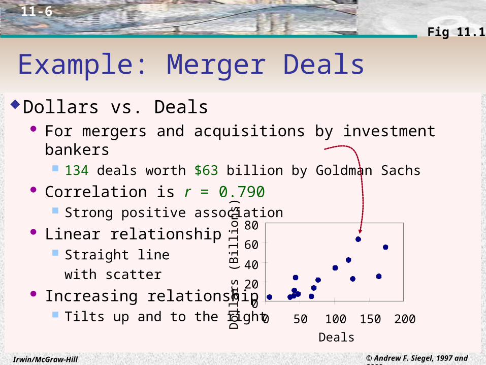
Example: Merger DealsDollars vs. Deals

For mergers and acquisitions by investment bankers 134 deals worth $63 billion by Goldman Sachs

Correlation is r = 0.790 Strong positive association

Linear relationship Straight line

with scatter Increasing relationship

Tilts up and to the right 0

20

40

60

80

0 50 100 150 200

Deals

Dol

lars

(B

illi

ons)

Fig 11.1.4


11-7

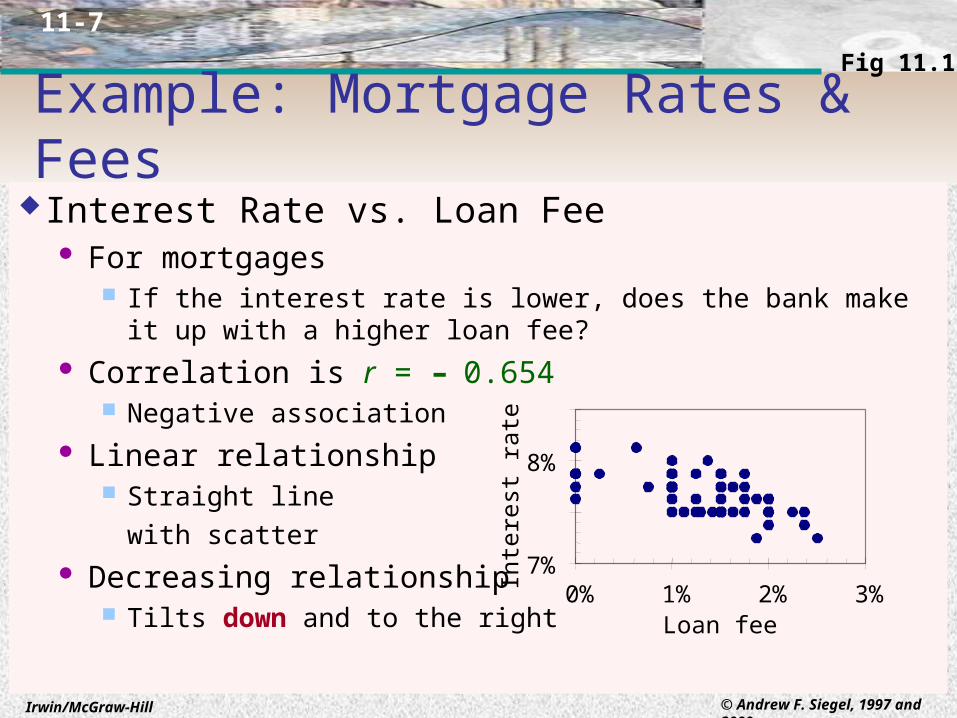
Example: Mortgage Rates & FeesInterest Rate vs. Loan Fee

For mortgages If the interest rate is lower, does the bank make it up with a higher loan

fee? Correlation is r = – 0.654

Negative association Linear relationship

Straight line

with scatter Decreasing relationship

Tilts down and to the right

7%

8%

0% 1% 2% 3%Loan fee

Inte

rest

rat

e

Fig 11.1.5


11-8

Example: The Stock MarketToday’s vs. Yesterday’s Percent Change

Is there momentum? If the market was up yesterday, is it more likely to be up today? Or is each

day’s performance independent? Correlation is r = 0.11

A weak relationship? No relationship?

Tilt is neither

up nor down

Fig 11.1.7

-3%

-2%

-1%

0%

1%

2%

3%

-3% -2% -1% 0% 1% 2% 3%

Yesterday's change

Toda

y's

chan

ge


11-9

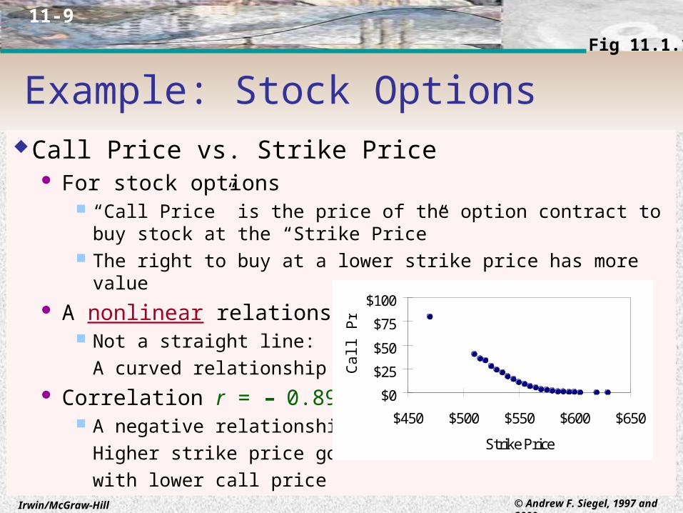
Call Price vs. Strike Price For stock options

“Call Price” is the price of the option contract to buy stock at the “Strike Price”

The right to buy at a lower strike price has more value A nonlinear relationship

Not a straight line:

A curved relationship Correlation r = – 0.895

A negative relationship:

Higher strike price goes

with lower call price

Example: Stock OptionsFig 11.1.10

$0

$25

$50

$75

$100

$450 $500 $550 $600 $650

Strike Price

Cal

l Pri

ce


11-10

Example: Maximizing YieldOutput Yield vs. Temperature

For an industrial process With a “best” optimal temperature setting

A nonlinear relationship Not a straight line:

A curved relationship Correlation r = – 0.0155

r suggests no relationship But relationship is strong

It tilts neither

up nor down

120

130

140

150

160

500 600 700 800 900

Temperature

Yie

ld o

f pr

oces

s

Fig 11.1.11


11-11

Example: TelecommunicationsCircuit Miles vs. Investment (lower left)

For telecommunications firms A relationship with unequal variability

More vertical variation at the right than at the left Variability is stabilized by taking logarithms (lower right)

Correlation r = 0.820

Fig 11.1.12,14

0

1,000

2,000

0 1,000 2,000Investment($millions)

Cir

cuit

mil

es(m

illi

ons)

15

20

15 20Log of investment

Log

of

mil

es

r = 0.957


11-12

Example: Bond Coupon and PricePrice vs. Coupon Payment

For trading in the bond market Bonds paying a higher coupon generally cost more

Two clusters are visible Ordinary bonds (value is from coupon) Flower bonds (value comes from estate tax treatment)

Correlation r = 0.867 for all bonds

Correlation r = 0.993 Ordinary bonds only

80

90

100

110

120

0% 5% 10% 15%

Coupon rate

Bid

pri

ce

Fig 11.1.15


11-13

Example: Cost and QuantityCost vs. Number Produced

For a production facility It usually costs more to produce more

An outlier is visible A disaster (a fire at the factory) High cost, but few produced

3,000

4,000

5,000

20 30 40 50Number produced

Cos

t

0

10,000

0 20 40 60Number produced

Cos

t

Outlier removed:More details,r = 0.869

r = – 0.623

Fig 11.1.16,17


11-14

Example: Salary and ExperienceSalary vs. Years Experience

For n = 6 employees Linear (straight line) relationship Increasing relationship

higher salary generally goes with higher experience Correlation r = 0.8667

Experience1510205

155

Salary303555224027 20

30

40

50

60

0 10 20 ExperienceSala

ry (

$tho

usan

d)

Mary earns $55,000

per year, and has

20 years of experience


11-15

The Least-Squares Line Y=a+bXSummarizes bivariate data: Predicts Y from X

with smallest errors (in vertical direction, for Y axis) Intercept is 15.32 salary (at 0 years of experience) Slope is 1.673 salary (for each additional year of experience, on

average)

10

20

30

40

50

60

0 10 20Experience (X)

Sala

ry (

Y)

Salary = 15.32 + 1.673 Experience


11-16

Predicted Values and ResidualsPredicted Value comes from Least-Squares Line

For example, Mary (with 20 years of experience)

has predicted salary 15.32+1.673(20) = 48.8 So does anyone with 20 years of experience

Residual is actual Y minus predicted Y Mary’s residual is 55 – 48.8 = 6.2

She earns about $6,200 more than the predicted salary for a person with 20 years of experience

A person who earns less than predicted will have a negative residual


11-17

Predicted and Residual (continued)

Mary earns 55 thousand

Mary’s predicted value is 48.8

10

20

30

40

50

60

0 10 20Experience

Sala

ry

Mary’s residual is 6.2


11-18

Standard Error of Estimate

Approximate size of prediction errors (residuals)Actual Y minus predicted Y: Y–[a+bX]

Example (Salary vs. Experience)

Predicted salaries are about 6.52 (i.e., $6,520) away from actual salaries

2

11 2

n

nrSS Ye

52.6 26

168667.01686.11 2

eS


11-19

Se (continued)Interpretation: similar to standard deviationCan move Least-Squares Line up and down by Se

About 68% of the data are within one “standard error of estimate” of the least-squares line (For a bivariate normal distribution)

20

30

40

50

60

0 10 20Experience

Sala

ry

(Least-squares lin

e) + S e

(Least-squares lin

e) – S e


11-20

Regression and Prediction ErrorPredicting Y as Y (not using regression)

Errors are approximately SY = 11.686

Predicting Y as a+bX (using regression) Errors are approximately Se = 6.52 Errors are smaller when regression is used!

This is often the true payoff for using regression

Coefficient of Determination R2

Tells what percent of the variability (variance) of Y is explained by X

Example: R2 = 0.86672 = 0.751 Experience explains 75.1% of the variation in salaries


11-21

Linear ModelLinear Model for the Population

The foundation for statistical inference in regression Observed Y is a straight line, plus randomness

Y = + X + Randomness of individuals

Population relationship, on average

{

X

Y


11-22

Why Statistical Inference?Because there can seem to be a relationship

when, in fact, the population is just randomSamples of size n = 10

from a population with no relationship (correlation 0) Sample correlations are not zero!

Due to the randomness of sampling

r = – 0.471 r = 0.089 r = 0.395


11-23

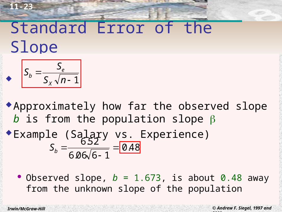
Standard Error of the Slope

Approximately how far the observed slope b is from the population slope

Example (Salary vs. Experience)

Observed slope, b = 1.673, is about 0.48 away from the unknown slope of the population

1

nS

SS

X

eb

48.0 1606.6

52.6

bS


11-24

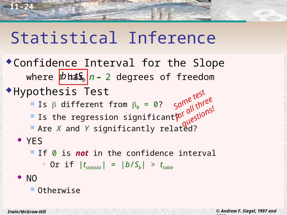
Statistical InferenceConfidence Interval for the Slope

where t has n – 2 degrees of freedomHypothesis Test

Is different from 0 = 0?

Is the regression significant? Are X and Y significantly related?

YES If 0 is not in the confidence interval

Or if |tstatistic| = |b/Sb| > ttable

NO Otherwise

btSb

Same test

for all three

questions!


11-25

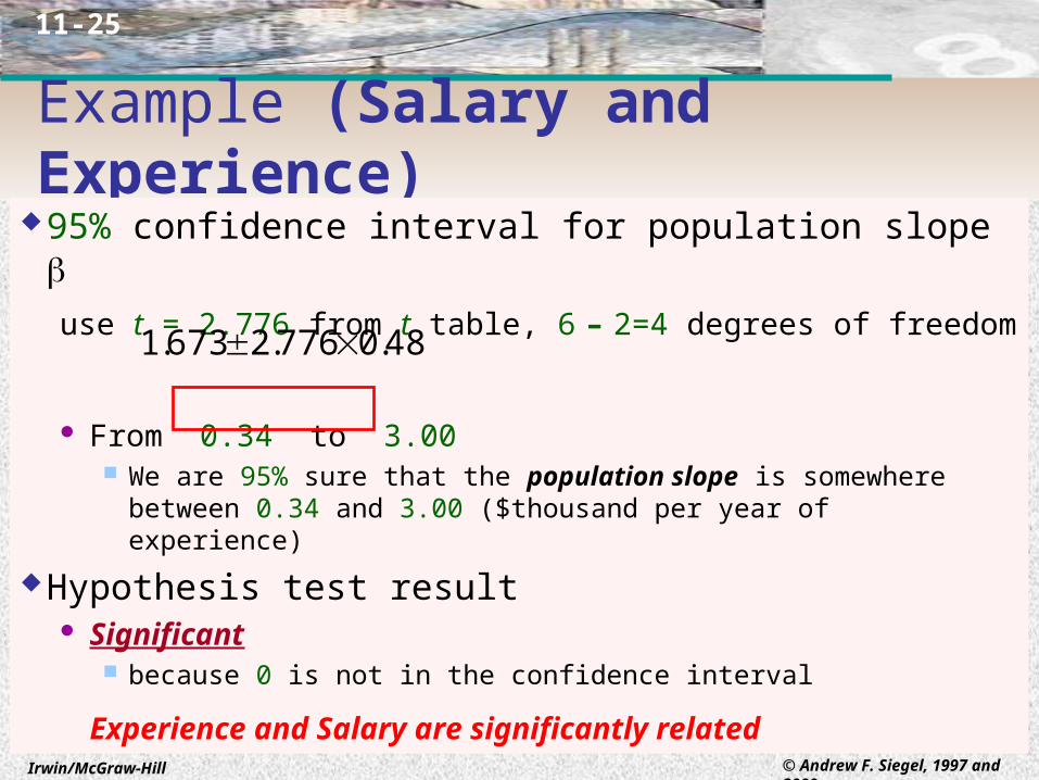
Example (Salary and Experience)95% confidence interval for population slope

use t = 2.776 from t table, 6 – 2=4 degrees of freedom

From 0.34 to 3.00 We are 95% sure that the population slope is somewhere between 0.34 and

3.00 ($thousand per year of experience)

Hypothesis test result Significant

because 0 is not in the confidence interval

Experience and Salary are significantly related

48.0776.2673.1


11-26

Regression Can Be MisleadingLinear Model May Be Wrong

Nonlinear? Unequal variability? Clustering?Predicting Intervention from Experience is Hard

Relationship may become different if you interveneIntercept May Not Be Meaningful

if there are no data near X = 0Explaining Y from X vs. Explaining X from Y

Use care in selecting the Y variable to be predictedIs there a hidden “Third Factor”?

Use it to predict better with multiple regression?

irwin/mcgraw-hill © andrew f. siegel, 1997 and 2000 11-1 regression and time series chapter 11...

Documents

irwinmcgrawhill andrew

right r

relationship tilts

negative relationship

nonlinear relationship

weak relationship

interpreting correlation

price example