ismael sanz and francisco j. velázquez european economy group

ISSN 0111-1760

THE COMPOSITION OF PUBLIC EXPENDITURE AND GROWTH:

DIFFERENT MODELS OF GOVERNMENT EXPENDITURE

DISTRIBUTION BY FUNCTIONS.

Ismael Sanz and Francisco J. Velázquez European Economy Group-UCM and FUNCAS*

No. 0115

August, 2001 Correspondence to: (*) Ismael Sanz ([email protected]), Francisco J. Velázquez ([email protected]) European Economy Group Facultad de Ciencias Económicas y Empresariales Universidad Complutense de Madrid.Campus de Somosaguas 28223 Madrid. Spain Department of Economics University of Otago PO Box 56 Dunedin NEW ZEALAND For copies of Discussion Paper, email requests to: [email protected]

2

The composition of public expenditure and growth: Different models of

government expenditure distribution by functions.

Ismael Sanz and Francisco J. Velázquez European Economy Group-UCM and FUNCAS*

August, 2001

Abstract

This paper provides a brief survey of the influence on economic growth of

the composition of public expenditure by functions, concluding that countries tend

towards a similar distribution in the steady state. In this light, we explore the

existence of convergence in the structure of government spending in the OECD

countries for the period 1970-1997 and the prospects of this process persisting in

the future. The results obtained through the dissimilarity index, using the usual

convergence indicators, and by means of cluster analysis point to the existence of

a convergence process in the structure of government expenditure by functions.

Nevertheless, we find that countries are approaching different equilibrium states in

which two main models can be differentiated: one for some of the State members

of the European Union (EU), and the other for almost the rest of the OECD

countries. This suggests that there exist individual factors that impede

convergence to a single distribution in the long run.

JEL: H500, H600. Keywords: Government spending, clusters, convergence, functions of public expenditure, OECD. (*) Ismael Sanz ([email protected]), Francisco J. Velázquez ([email protected])

European Economy Group

Facultad de Ciencias Económicas y Empresariales

Universidad Complutense de Madrid.Campus de Somosaguas

28223 Madrid. Spain

3

Acknowledgements

We are grateful to Stephen Knowles, Carmela Martin and Dorian Owen for their

helpful and interesting comments and suggestions on this paper. Part of this

research was undertaken while the first author was a Visiting Research Fellow of

the Economics Department of the University of Otago. We are grateful for the

hospitality received and all the research facilities provided. Financial support from

the European Economy Group (Universidad Complutense de Madrid) and FUNCAS

is gratefully acknowledged. We would like to thank also the participants of the

75th International Conference: Policy Modelling for European and Global Issues

Brussels, July 2001, and 57th Congress of the International Institute of Public

Finance: The Role of Political Economy in the Theory and Practice of Public

Finance, Linz, August 2001, for their comments and suggestions.

4

INTRODUCTION

Since 1980, several articles have analysed the impact of the size of the

public sector on economic growth without obtaining conclusive results. 1 With the

development of endogenous growth models, the composition of government

expenditures, above all the percentage of these allocated to productive

expenditures, has been considered as relevant determinant of growth (Barro,

1990). There is a developing consensus about the positive effect of public

investment and the negative effect of public consumption on economic growth

(Sturm, 1998).

However, it has been only recently that the literature has begun to evaluate

the influence of the functional breakdown of government spending on growth (Chu

et al.,1995; Devarajan et al., 1996; Tanzi and Zee, 1997; Bleaney et al., 1999).

In this sense, the purpose of the research, of which this article forms part, is to

estimate the elasticities of economic growth with respect to the components of

public expenditures using a broader disaggregation than productive versus non-

productive components.2

Hence, and as a prior step to the formulation of an endogenous growth

model, this article evaluates the convergence of the functional breakdown of public

expenditures in the developed countries in the last three decades. The results

obtained will be of interest to analyse, firstly, the disparities of public expenditure

composition as a factor explaining the differences in long-run economic growth

rates, and secondly, whether the progress in co-ordination of fiscal policy

1 Agell, Lindh and Ohlsson (1997 and 1999), obtain this conclusion in their survey of the effects of fiscal policy on economic growth, including their own empirical analysis. 2 For example, among productive expenditures Bleaney et al., (1999) include those devoted to health, general administration services, public order, education, defence, transport and communication and housing. Therefore, non-productive functions would be social security, recreation, culture and religious services, and all the economic services except transport and communication.

5

stemming from growing economic globalisation has affected the functional

breakdown of public expenditure.

With this purpose, section 2 examines some theoretical models of the

influence on growth of the composition of public expenditure by functions. From

this framework, we infer that governments of countries at a similar stage of

development should move towards the same distribution of public expenditure.

This result leads to an analysis of the evolution of convergence in the government

spending structure of OECD countries.

With this aim, in section 3 we explore the evolution of the size and

composition of public expenditure during the period 1970-1997. Afterwards,

section 4 evaluates convergence in the composition of public expenditure adapting

for the analysis the usual indicators in the literature of convergence in per capita

income. Moreover, we investigate if there is a margin for future alignment of the

share of each functional category in the total amount of public expenditures in the

OECD countries. In section 5, we identify if countries converge to different models

of government spending structure. Finally, in section 6, we set out the main

conclusions obtained.

2. THE COMPOSITION OF PUBLIC EXPENDITURE BY FUNCTIONS AND

ECONOMIC GROWTH.

The literature on the influence of government spending on growth has

focused its interest on the impact of the overall size of government spending. It

has been only recently that the literature has begun to evaluate the influence of

the composition of public expenditure on growth. Following Devarajan et al.

(1996) and Barro (1990), we will draw some conclusions about the pattern

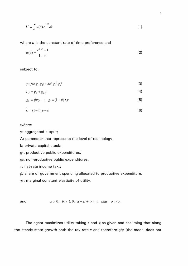
expected of the functional breakdown of public expenditure. Devarajan et al.

consider a representative infinite-lived agent that chooses consumption c and

capital k to maximize utility:

6

dtecuUpt−∞

∫= 0)( (1)

where p is the constant rate of time preference and

σ

σ

−−

=−

11)(

1ccu (2)

subject to:

γβα2121 ),,( ggkAggkfy == (3)

21 ggy +=τ ; (4)

ygyg τφτφ )1(; 21 −== (5)

cyk −−=•

)1( τ (6)

where:

y: aggregated output;

A: parameter that represents the level of technology.

k: private capital stock;

g1: productive public expenditures;

g2: non-productive public expenditures;

τ: flat-rate income tax,:

φ: share of government spending allocated to productive expenditure.

-σ: marginal constant elasticity of utility.

and 0 .01;0,; >=++≥> σγβαγβα and

The agent maximizes utility taking τ and φ as given and assuming that along

the steady-state growth path the tax rate τ and therefore g/y (the model does not

7

allow for deficit financing) is constant,3 Devarajan et al. (1996) arrive at an

interesting condition. They show that an increase in the share of the productive

component of public expenditure,φ, will raise the steady-state growth rate if:

<

− γβ

φφ

1 (7)

Note, that the effect on growth of a shift towards more productive

expenditure will depend both on the relative elasticities and the initial shares of

each expenditure. These authors point out that this model can be extended to N

types of government expenditure. In this more general case, the condition (7) for a

positive effect on growth of a shift from type f towards type s spending would be

(Devarajan et al. p.319) :

s

s

f

f

φβ

φ

β> (8)

Where βf is the elasticity of y with respect to type f public expenditure and φf

is the share of type f spending in total public expenditure. We will apply this

condition for the case of OECD countries and use the Classification of the

Functions of the Government (COFOG, see United Nations, 1981). We will

consider eight different types of expenditures grouped according to the

classification introduced by Oxley and Martin (1991) and that already mentioned of

Bleaney et al. (1998) (see Appendix 1). Thus, productive expenditure includes:

pure public goods (general administrative services and public order and safety, and

defence); merit goods (health, education and housing); and one component of

economic services (transport and communications). Non-productive expenditure

includes transfers (social welfare) and the rest of economic services and other

3 Barro (1990) assumes that the government carries out no production and owning no capital, but just buys from the private sector a flow of output, which enters as a input in the private production function. However, Cashin (1995) does include public capital goods of the public spending as a stock and public transfers as a flow on the private production.

8

(recreational, cultural and religious affairs, and other functions, essentially interest

payments).

Assume that the elasticies for each type of expenditure are the same across

countries.

.8...,,2,1:;, fjifjfi ∀= ββ (9)

This assumption is implicitly made when empirically estimating this model

with cross-section or panel data, as in fact is done by Devarajan et al.. In defence

of this assumption, note that we are not working with developing countries at very

different stage of development, but with OECD countries, which are more

homogenous. Furthermore, the growing globalisation process in this area has

harmonised the macroeconomic conditions faced by all the countries and the

productive structure of these economies.

Then Equation (8) can be written as:

is

fi

js

jf

is

if

φφ

ββ

ββ

>= or js

jf

js

jf

is

if

φφ

ββ

ββ

>= (10)

By assumption the ratio between the elasticies of output with respect to the

two functions is the same for every possible combination of pairs of countries.

This means that the equilibrium, at which no shifts in any particular function can

increase growth in the long term, will be the same for all countries:

jiandsfjisfand fjfijfifis

if

is

fi ,,,;,; ****

∀=∀∀== ⇒ φφβββ

β

φ

φ

9

So approaching the equilibrium distribution of public expenditure implies

convergence to the same structure. In the rest of this work we will try to analyse

if this is the case for the OECD countries in the period 1970-1997.

3. THE SIZE AND COMPOSITION OF GOVERNMENT EXPENDITURE.

Public expenditure has increased its share in the GDP of OECD countries

from 32% in 1970 to almost 40% in 1997. However, this expansion has

fluctuated in the course of the three decades (Figure 1). In fact, there are four

distinguishable sub-periods. The first covers the decade of the seventies and the

early years of the eighties, in which the public sector increased its share

constantly, continuing the tendency started in World War II. This trend is

interrupted in 1983 until the end of the eighties, which is the second period. The

share of public expenditure in GDP stabilised as a consequence of the threat to the

sustainability of public finances at the levels attained in the previous sub-period

(Saunders and Klau, 1985; Oxley et al., 1990).

At the beginning of the nineties public expenditure increased its importance

again until 1995, the peak for the whole period, coinciding with the end of the

economic crisis.4 Thereafter, there is a reduction in the public expenditure share as

a result of the fiscal discipline implemented in the OECD countries (Lindbeck,

1997). Certainly, EU Member States signed the Stability and Growth Pact, 1996,

which constrained their public deficits and debt levels, whilst the United States

adopted the Balanced Budget Amendment.

4 Saunders (1993) and Tanzi and Schuknecht (2000) analyse in detail the trends in the size and scope of the public sector in developed countries, and give some explanations about its determinants.

10

Figure 1. Trends in Public Expenditure in the OECD countries (1970-1997, % GDP)

15

20

25

30

35

40

45

50

55

60

1970 1972 1974 1976 1978 1980 1982 1984 1986 1988 1990 1992 1994 1996 1998

% G

DP

European Union

OECD

United States

Japan

Source: OECD

Thus, it will be of great interest to examine whether the OECD member states

have harmonised the functional distribution of their public expenditures in these

sub-periods.5 For this purpose, we computed an index, SIG, that measures the

dissimilarity of the public expenditure structure by functions:

−

= ∑

∑∑

∑

∑∑

=

= =

=

=

=

n

i

s

f

n

ifit

n

ifit

s

ffit

fit

s

ft

GG

GG

SIG ns 1

1 1

1

1

1111

(11)

where:

5 Nevertheless, we have considered the decade of the nineties as one sub-period, since the decrease in the public expenditure share in GDP applied only for two years: 1996 and 1997.

11

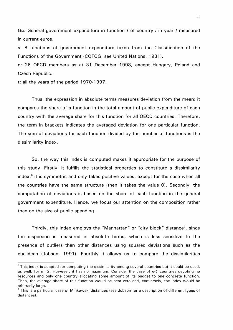
Gfit: General government expenditure in function f of country i in year t measured

in current euros.

s: 8 functions of government expenditure taken from the Classification of the

Functions of the Government (COFOG, see United Nations, 1981).

n: 26 OECD members as at 31 December 1998, except Hungary, Poland and

Czech Republic.

t: all the years of the period 1970-1997.

Thus, the expression in absolute terms measures deviation from the mean: it

compares the share of a function in the total amount of public expenditure of each

country with the average share for this function for all OECD countries. Therefore,

the term in brackets indicates the averaged deviation for one particular function.

The sum of deviations for each function divided by the number of functions is the

dissimilarity index.

So, the way this index is computed makes it appropriate for the purpose of

this study. Firstly, it fulfills the statistical properties to constitute a dissimilarity

index:6 it is symmetric and only takes positive values, except for the case when all

the countries have the same structure (then it takes the value 0). Secondly, the

computation of deviations is based on the share of each function in the general

government expenditure. Hence, we focus our attention on the composition rather

than on the size of public spending.

Thirdly, this index employs the “Manhattan” or “city block” distance7, since

the dispersion is measured in absolute terms, which is less sensitive to the

presence of outliers than other distances using squared deviations such as the

euclidean (Jobson, 1991). Fourthly it allows us to compare the dissimilarities

6 This index is adapted for computing the dissimilarity among several countries but it could be used, as well, for n=2. However, it has no maximum. Consider the case of n-1 countries devoting no resources and only one country allocating some amount of its budget to one concrete function. Then, the average share of this function would be near zero and, conversely, the index would be arbitrarily large. 7 This is a particular case of Minkowski distances (see Jobson for a description of different types of distances).

12

among different functions since the deviation is computed relative to the mean of

each one. In fact, the index has a consistent decomposition allowing the

examination of the contribution of each function to the total dissimilarity. 8 Finally,

the deviation is computed giving the same weight to each country, reflecting a

generalised trend rather than changes in a small sample of big countries.

The data source used is the OECD: National Accounts. Volume II: Detailed

Tables. The authors have chosen this source because the data are consolidated for

all levels of public administration and are constructed on an accrual basis.9

Nevertheless, we have also used national agencies, data, OECD and World Bank

country reports, Eurostat: General Government Accounts and Statistics and the

IMF’s Government Finance Statistics,10 in order to complete the time series.

Finally, for the case of France, the data for the period 1970-1974 have been taken

from Sanz (1993), whilst for Japan some missing data have been extrapolated.

TABLE 1. Dissimilarity Indexes of the functions of government expenditure in the OECD 1970-1997 70-79 80-89 90-97 Pure Public Goods Public Services 0.32 0.30 0.26 Defence 0.56 0.55 0.51 Merit Goods

8 Other distances, suchas the chi-square (Lebart, Morineau and Fenelon, 1982), weight the sum of deviations by the inverse share: i.e, giving more importance to the variation of the smaller functions such as housing and transport and communication. The chi-square independence test of Pearson is based on this distance. 9 We have taken into account the criticisms contained in Florio (1998) about the lack of homogeneity in the treatment of interest payments, comparing this item with other international and national sources. 10 The data provided by the IMF are not generally consolidated for all levels of government. Therefore, it was necessary to subtract the transfers between different administrations (see Easterly and Rebelo, 1993 for a discussion about the limitations of the data provided by IMF). In addition to this, the Government Finance Statistics calculates the data using cash basis accounting. Hence, only the trend of the data of this source –which in the long term approximates the evolution of the data on an accrual basis- has been employed to enlarge time series.

13

Health 0,27 0.26 0.26 Education 0.22 0.16 0.19 Housing 0.50 0.46 0.48 Economic Services and Others Transport and Communications 0.49 0.44 0.39 Other 0.43 0.39 0.38 Transfers Social Welfare 0.34 0.33 0.31 Total 0.39 0.36 0.35 Source: own calculations on the basis of OECD, National Agencies, World Bank, IMF and Eurostat data

So, as can be seen in Table 1, the dissimilarity among OECD countries’

public expenditure distribution has been reduced in the last three decades.11

However, this process took place during the fiscal expansion of the seventies,

whilst in the eighties and nineties it ceased. In fact, the hypothesis of

independence of government expenditure structure by functions is rejected with a

p-value of 0,00 for every year. That is, the distribution of public spending among

countries is still significantly different. Moreover, though every function has

decreased its dissimilarity, this development was not homogenous for all. Thus,

merit goods and transfers show a negligible decline. Nevertheless, this category

still has the most similar shares among OECD countries, above all, education.12 On

the other hand, economic services and others, and pure public goods13 have

converged constantly and significantly. Among these, pubic services is the

function showing the fastest harmonisation process.

11 The same conclusion is obtained using chi-square distance: total inertia decreased from 0,20 to 0,12, where 0 indicates total similarity. 12 O’Higgins (1988) reached the same conclusion: public education expenditures show small variability in OECD countries. 13 This result is in line with Atkinson and Van den Noord (2001), who point out that these two categories have been stable in almost all OECD countries during the decades of the eighties and nineties. Only the countries with higher shares in the seventies, such as Japan, Norway, Germany, Italy, Australia, United States and United Kingdom, have decreased significantly these types of expenditure. Accordingly the dissimilarity index decreased. On the other hand, the evolution of merit goods and transfers has been very similar for all the countries: a stabilisation process after the substantial increase of the seventies (Saunders, 1993, Tanzi and Schuknecht, 2000)

14

The evolution described for the convergence of public expenditure

distribution coincides with the one drawn out for the size of the public sector.

Actually, there is a negative and significant correlation coefficient (–0,86) between

the annual share of public expenditure in GDP in the OECD and the annual total

dissimilarity index computed above for the period 1970-1997. This result indicates

that during fiscal expansion the countries harmonised their functional distribution,

while for the years characterised by fiscal discipline the dissimilarity increased.

That is, the composition of fiscal adjustment differs among OECD countries, so

that governments reduce the share of distinct functions when they decide to

decrease public deficits. This is an important difference with the behaviour of

public expenditure distribution by economic type, which takes into account if it is

consumption, investment or transfers. In fact, fiscal adjustments take place

reducing investments because, as pointed out by Kamps (1985), Roubini and

Sachs (1989) and Oxley and Martin (1991), political reasons make it easier to

diminish this type of expenditure.14

4. CONVERGENCE IN THE COMPOSITION OF GOVERNMENT EXPENDITURE

The analysis of convergence in the composition of government expenditure in

OECD countries during the period 1970-1997 will be carried out by means of the

usual approach in the literature on per capita income convergence (Barro and Sala-

i-Martin, 1990 and 1992, De la Fuente, 2000). We will adapt this analysis to the

examination of the functional distribution of public spending. Thus, we start with

the examination of β convergence, with the object of evaluating whether countries

that have a higher share in one particular function increase (decrease) this

14 Henrekson (1988) in the case of Sweden and Sturm (1998) for the OECD member states find that fiscal adjustment affects particularly investments. However, Alesina and Perotti (1995) show that adjustments based on social transfers and the wage component of public consumption are more persistent than the ones based on investments reduction and earned income tax increases. In addition, and contrary to general belief but in line with the suggestions with Aubin et al (1988), Alesina et al (1998) point out that governments implementing the first type of adjustment obtain stronger electoral support.

15

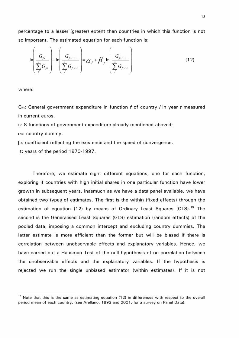
percentage to a lesser (greater) extent than countries in which this function is not

so important. The estimated equation for each function is:

+=

−

∑∑∑ −

−

−

−s

ftfi

tfi

ffis

ftfi

tfis

ffit

fit

G

G

G

G

G

G

1,

1,

1,

1, lnlnln βα (12)

where:


in current euros.

s: 8 functions of government expenditure already mentioned aboved;

αfi: country dummy.

βf: coefficient reflecting the existence and the speed of convergence.

t: years of the period 1970-1997.

Therefore, we estimate eight different equations, one for each function,

exploring if countries with high initial shares in one particular function have lower

growth in subsequent years. Inasmuch as we have a data panel available, we have

obtained two types of estimates. The first is the within (fixed effects) through the

estimation of equation (12) by means of Ordinary Least Squares (OLS).15 The

second is the Generalised Least Squares (GLS) estimation (random effects) of the

pooled data, imposing a common intercept and excluding country dummies. The

latter estimate is more efficient than the former but will be biased if there is

correlation between unobservable effects and explanatory variables. Hence, we

have carried out a Hausman Test of the null hypothesis of no correlation between

the unobservable effects and the explanatory variables. If the hypothesis is

rejected we run the single unbiased estimator (within estimates). If it is not

15 Note that this is the same as estimating equation (12) in differences with respect to the overall period mean of each country, (see Arellano, 1993 and 2001, for a survey on Panel Data).

16

rejected we proceed with the GLS estimates because in addition to being unbiased

they will be the most efficient.

If the coefficient β takes a negative and significant value, there has been a

convergence process in the function. Still, there are two types of β-convergence:

conditional and absolute. The former is less restrictive, since it takes into account

other specific factors affecting functional shares in each country. In equation (12)

the fundamentals of economy i are picked up by the country dummies, assuming

these effects remain constant over time.16 The latter requires the existence of

convergence even without considering other variables. So, there would be absolute

convergence in two cases: firstly if the GLS estimator is unbiased and hence we

do not include any other variable apart from the previous year’s share as an

explanatory variable for the change of rate; and secondly if only the within

estimator is unbiased, but we can not reject the hypothesis of country dummies

being equal for all the countries (De la Fuente, 2000). In this case all the countries

will converge to the same steady state.

Thus, in the steady state:

0lnln1,

1, =

−

∑∑ −

−s

ftfi

tfis

ffit

fit

G

G

G

G (13)

and the system is stable when β varies between 0 and –1. If we substitute in (12)

we obtain a value for the equilibrium share of each function:

−=

∑ f

fis

ffi

fi

G

G

β

α

*

ln and

( )f

fi

e

G

Gs

ffi

fi βα

−

=

∑

*

(14)

16 We are aware that there are many factors determining the distribution of public expenditures that are not constant over time, but with this specification we try to do a descriptive analysis of the pattern of functional shares in total government spending. The factors underlying individual effects will be the subject of the next step of our investigation.

17

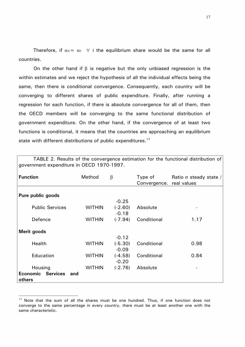
Therefore, if αfi= αf ∀ i the equilibrium share would be the same for all

countries.

On the other hand if β is negative but the only unbiased regression is the

within estimates and we reject the hypothesis of all the individual effects being the

same, then there is conditional convergence. Consequently, each country will be

converging to different shares of public expenditure. Finally, after running a

regression for each function, if there is absolute convergence for all of them, then

the OECD members will be converging to the same functional distribution of

government expenditure. On the other hand, if the convergence of at least two

functions is conditional, it means that the countries are approaching an equilibrium

state with different distributions of public expenditures.17

TABLE 2. Results of the convergence estimation for the functional distribution of government expenditure in OECD 1970-1997. Function

Method

β

Type of Convergence.

Ratio σ steady state / real values

Pure public goods

Public Services

WITHIN

-0.25 (-2.60)

Absolute

-

Defence

WITHIN

-0.18 (-7.94)

Conditional

1.17

Merit goods

Health

WITHIN

-0.12 (-5.30)

Conditional

0.98

Education

WITHIN

-0.09 (-4.58)

Conditional

0.84

Housing

WITHIN

-0.20 (-2.76)

Absolute

-

Economic Services and others

17 Note that the sum of all the shares must be one hundred. Thus, if one function does not converge to the same percentage in every country, there must be at least another one with the same characteristic.

18

Transport and Communications

WITHIN

-0.16 (-4.46)

Conditional

0.79

Other

WITHIN

-0.09 (-2.88)

Absolute

-

Transfers

Social Welfare

WITHIN

-0.13 (-3.39)

Conditional

1.13

White´s (1980) heteroscedasticity-consistent t-statistics are given in parentheses.

Equation (14) allows us to estimate these equilibrium states and to evaluate

the margin for further convergence. This will be done by means of the comparison

of the standard deviation of the shares estimated in the equilibrium state for every

country in a particular function and the standard deviation of the real shares of this

function for every country in the last year available (1997).

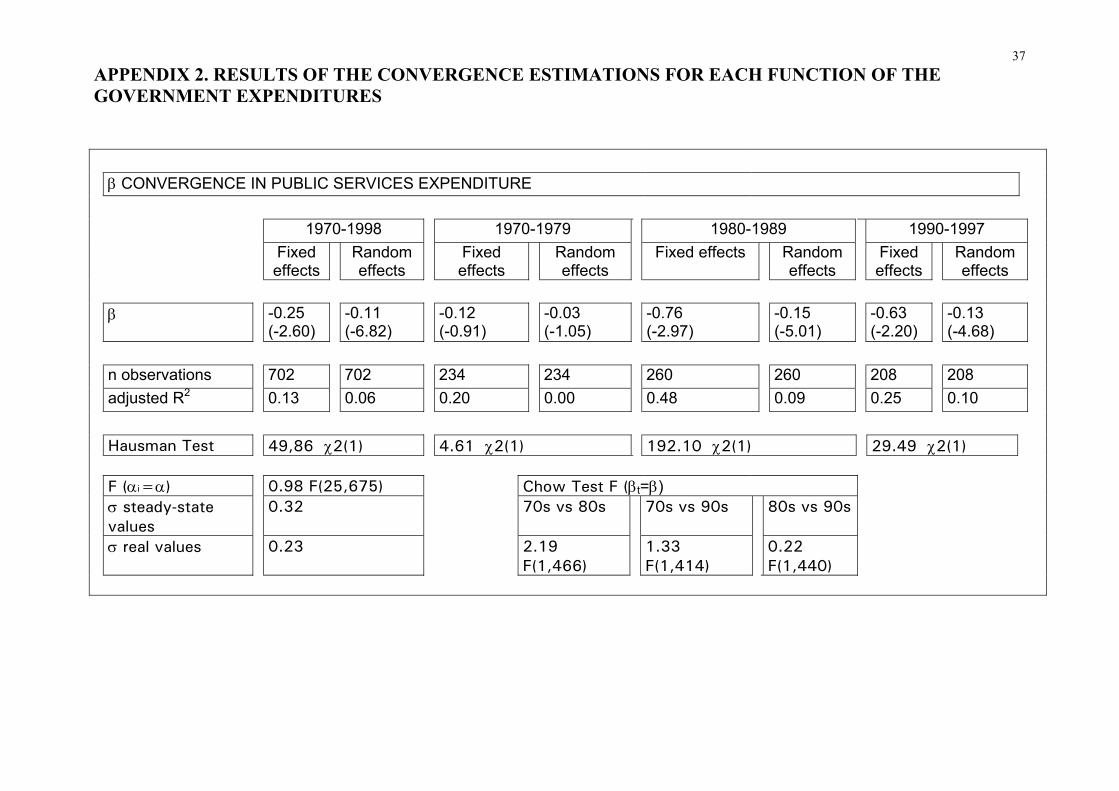
The results given in Table 2 show that there has been a convergence

process in all the functions.18 However, the consistent estimator for all the cases is

the within estimator as can be inferred from the rejection of the null hypothesis of

the Hausman Test. Moreover this convergence is absolute only in three cases:

public services, housing and other expenditures. For all other functions, the F test

rejects the hypothesis that the individual effects are the same for every country;

they converge to different equilibrium states with distinct distributions of public

expenditure. Country dummies reflect idiosyncratic effects that impede

convergence to the identical composition of public expenditure. By functions,

public services is again the one converging fastest (–0,25). The results shown in

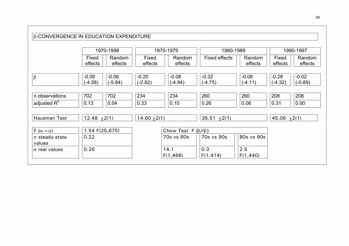
the last column of Table 2, suggest there is still some margin for convergence that

only in education, transport and communications expenditures since the disparities

of the equilibrium state shares for these functions are smaller than for the real

shares of 1997. Health is very close to the steady state. On the other hand, social

welfare and defence could at some point begin to diverge if they continue the

patterns shown in the period 1970-1997.

18 The detailed results can be found in appendix 2.

19

However, in computing the equilibrium state, we are assuming not only that

there is no variation in the individual effects reflecting fundamental characteristics

of the country i, but also that β remains stable over the whole period.

Nevertheless, political and socio-economic changes can affect the preference of

governments for different expenditure functions.19 Hence, we have tested by

means of the Chow Test the equality of the parameters in the three decades to

explore if there are different convergence patterns over the period.

The analysis of the test on the equality of the speed of convergence is

shown in Table 3. Seven of the functions show a statistically similar speed of

convergence for most of the period. Interesting is the fact that, for the case of

expenditures showing absolute convergence, we cannot reject the hypothesis of

having identical speeds of convergence for the three decades. In addition,

education, health, transport and communications, which have less variability in the

steady state than in 1997, have a stable coefficient at least in the last two

decades. These results confirm that these functions have still some margin to

continue converging. On the other hand, social welfare and, above all, defence,

with higher dispersion in the equilibrium, have had structural breaks at least in the

last decade. In fact it seems as if these functions have reduced significantly the

speed of convergence achieved in the eighties, giving the first indications of having

no more margin to converge and even to start diverging.

TABLE 3. Speed of convergence of each function in the three decades

70-79 80-89 90-97 70s vs 80s 70s vs 90s 80s vs 90s Pure public goods Public services

-0.13

(-0.91)

-0.76 (-2.97)

-0.63

(-2.20)

=

=

=

Defence

-0.22

(-6.66)

-0.40 (-6.96)

-0.35

(-5.32)

≠

≠

≠

Merit goods 19 Sturm (1998) points out that the colour or the strength of the governments can influence the composition of public expenditures, although he does not find any influence of these variables on the share of capital investment.

20

Health -0.24 (-3.53)

-0.39 (-4.59)

-0.40 (-3.56)

≠ = =

Education

-0.20

(-2.82)

-0.32 (-4.75)

-0.28

(-4.32)

≠

=

=

Housing

-0.37

(-3.01)

-0.36 (-4.10)

-0.43

(-2.39)

=

=

=

Economic services and others

Transport and Communications

-0.35

(-3.92)

-0.27 (-3.40)

-0.31

(-3.73)

=

=

=

Other

-0.31

(-4.93)

-0.33 (-5.40)

-0.30

(-2.65)

=

=

=

Transfers Social Welfare

-0.68

(-4.73)

-0.46 (-2.97)

-0.20

(-1.00)

=

=

≠

Nevertheless, the existence of β-convergence is a necessary but not

sufficient condition for convergence. It is σ-convergence that ensures there has

been a convergence process (Barro and Sala-i-Martin, 1992). For this reason, we

have computed the standard deviation of the logarithm of the specialisation index

of each function. In the context of this work, σ-convergence explores if the

dispersion among the relative shares of the functions of government expenditures

among OECD countries has been reduced. Computing the standard deviation of the

specialisation index gives the possibility of comparing the dispersion of the

different functions.

Thus

21

2

1 1

1

1

1 1

1

1

1

))(log(log1

−

=

∑ ∑

∑

∑

∑ ∑

∑

∑∑

= =

=

=

= =

=

=

=

s

f

n

ifit

n

ifit

s

ffit

fit

s

f

n

ifit

n

ifit

s

ffit

fit

s

ift

G

G

G

G

mean

G

G

G

G

nσ

TABLE 4. σ-convergence of the shares of each function in the total amount of government spending relative to the OECD average (1970-1997). 70-79 80-89 90-97 Pure public goods Public services 0.29 0.26 0.24 Defence 0.69 0.69 0.58 Merit goods Health 0.34 0.39 0.40 Education 0.27 0.17 0.18 Housing 0.59 0.56 0.59 Economic services and others Transport and communications

0.42 0.40 0.36

Other 0.36 0.33 0.35 Transfers Social Welfare 0.43 0.44 0.35 Total 0.58 0.58 0.55

The results obtained for σ-convergence in Table 4, confirm the existence of

a harmonisation tendency in the functional distribution of government

expenditures, since the standard deviation has decreased in the three decades.

Moreover, the data confirms the existence of convergence in most of the functions

(all except health). The share of education expenditure is the most similar among

OECD countries, though, jointly with housing, having increased disparities in the

last decade as pointed out already with the dissimilarity index. Public services

again show the fastest harmonisation.

Finally, we have calculated the Kendall index with the object of analysing

whether there are significant changes in the rankings. This is known as γ-

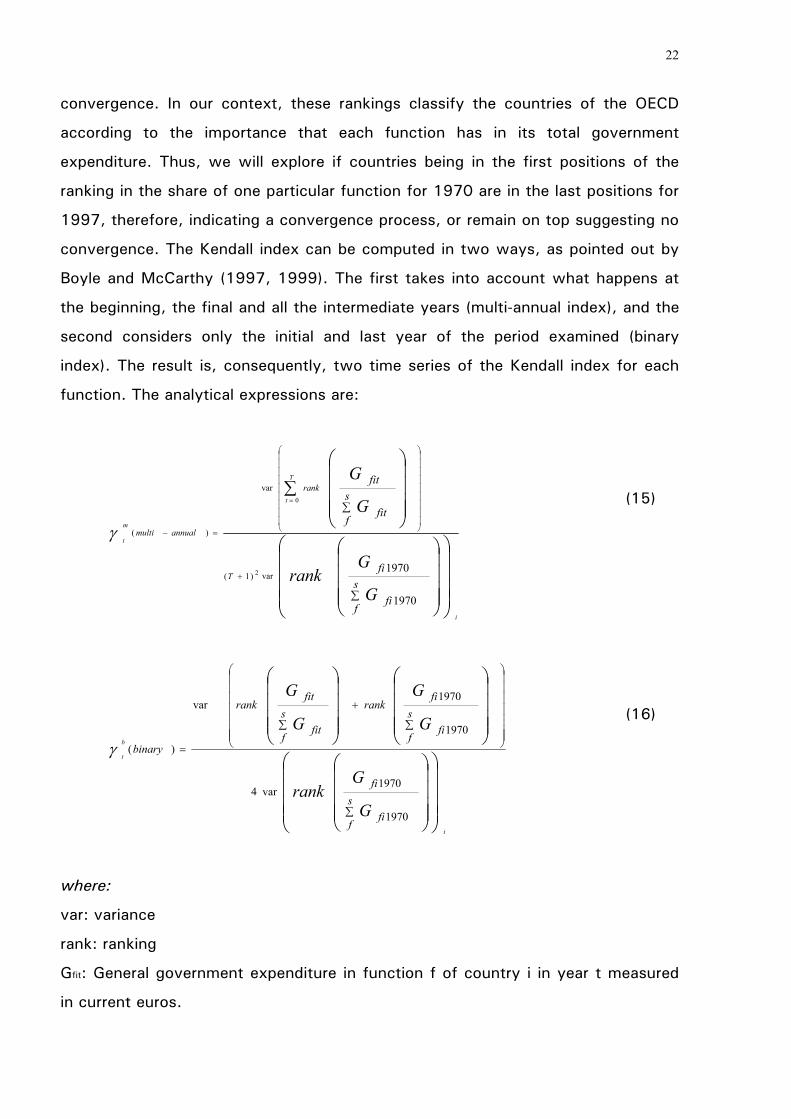
22

convergence. In our context, these rankings classify the countries of the OECD

according to the importance that each function has in its total government

expenditure. Thus, we will explore if countries being in the first positions of the

ranking in the share of one particular function for 1970 are in the last positions for

1997, therefore, indicating a convergence process, or remain on top suggesting no

convergence. The Kendall index can be computed in two ways, as pointed out by

Boyle and McCarthy (1997, 1999). The first takes into account what happens at

the beginning, the final and all the intermediate years (multi-annual index), and the

second considers only the initial and last year of the period examined (binary

index). The result is, consequently, two time series of the Kendall index for each

function. The analytical expressions are:

∑

∑

∑

+

=−

=

s

ffi

fi

s

ffit

fit

G

Grank

G

G

i

T

t

m

t

T

rank

annualmulti

1970

1970var)1(

var

)(

2

0

γ

(15)

∑

∑

+

∑

=

s

ffi

fi

s

ffi

firank

s

ffit

fitrank

binary

G

Grank

G

G

G

G

i

b

t

1970

1970var4

1970

1970var

)(γ

(16)

where:

var: variance

rank: ranking


in current euros.

23

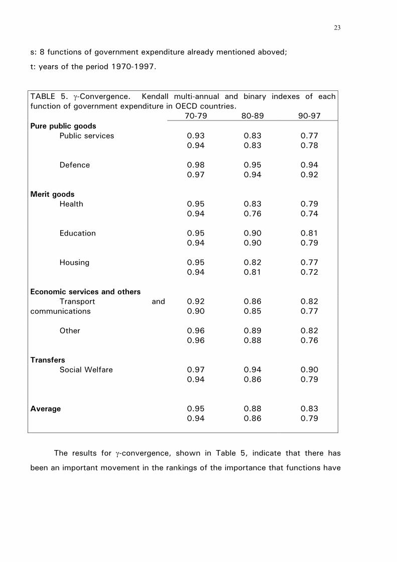
s: 8 functions of government expenditure already mentioned aboved;

t: years of the period 1970-1997.

TABLE 5. γ-Convergence. Kendall multi-annual and binary indexes of each function of government expenditure in OECD countries. 70-79 80-89 90-97 Pure public goods Public services 0.93

0.94 0.83 0.83

0.77 0.78

Defence 0.98

0.97 0.95 0.94

0.94 0.92

Merit goods Health

0.95 0.94

0.83 0.76

0.79 0.74

Education 0.95 0.94

0.90 0.90

0.81 0.79

Housing 0.95

0.94 0.82 0.81

0.77 0.72

Economic services and others Transport and communications

0.92 0.90

0.86 0.85

0.82 0.77

Other 0.96

0.96 0.89 0.88

0.82 0.76

Transfers Social Welfare 0.97

0.94 0.94 0.86

0.90 0.79

Average 0.95

0.94 0.88 0.86

0.83 0.79

The results for γ-convergence, shown in Table 5, indicate that there has

been an important movement in the rankings of the importance that functions have

24

in each country, measured as the share in total public expenditure.20 Thus, public

services is again the function showing the greatest convergence. Health and

housing reflect also a relevant change in their ranking during the period 1970-

1997. In contrast, the expenditure having most disparities at the beginning of the

period (defence) and the larger share in the total public spending (social welfare)

present less mobility in their particular classifications. These characteristics make it

more difficult for the countries to change positions in the ranking. Furthermore, the

two functions mentioned reflect idiosyncratic and institutional factors, such as the

role of the State in economic activity and the creation of the Welfare State.

In short, the convergence analysis reveals that there has been an alignment

of functional distributions among OECD countries in the period 1970-1997.

Nevertheless in 1997 the margin for future convergence seems to be very small,

that is, functions appear to be close to the steady states, which are different for

each country.

5. CLUSTERS

Because we have found individual effects that impede the approach of

OECD countries towards a single distribution, we will explore if there is, at least,

convergence to more than one distribution of public expenditure structure by

functions. For this purpose, countries of the OECD will be classified using a

combination of hierarchical and non-hierarchical methods of cluster analysis, so

that we can benefit from the advantages of each method while avoiding the bias

of either. (Milligan, 1980)

20 The Kendall indexes obtained are significant at the 1% level until 1990. Afterwards, several of them are significant at the 2.5% level. With n countries, the test statistic is distributed as a chi-square with n-1 degrees of freedom under the null hypothesis of independence between rankings of each year.

25

Along these lines, in the first stage, we use Ward’s hierarchical method21

with the squared euclidean distance.22 With this first step the ideal number of

clusters is obtained–using the stopping rule (Milligan and Cooper, 1985)23- and the

centroids of each one. In a second step, we use the most generalised non-

hierarchical method, k-means (MacQueen, 1967), using the centroids of the first

step as the initial seed points of the clusters. Thus we avoid the disadvantages of

the non-hierarchical methods (its sensitivity to initial centroids and the arbitrary

choice of the number of clusters, Johnson and Wichern, 1998), since both

parameters are introduced from the results obtained from the hierarchical method

which does not require any ex ante information. Meanwhile we benefit from the

possibility offered by non-hierarchical methods of switching the cluster’s

membership of early combinations, not to mention that they are less sensitive to

outliers and to the distance measure chosen (Hair and Black, 2000). Combining

both methods makes it possible to observe different distributions of government

expenditure by functions (represented by the centroids) and if there has been a

convergence process among clusters and countries.

In addition, the data have been standardised with the purpose, firstly, of

avoiding larger functions such as social welfare and other expenditures dominating

in the formation of clusters. Secondly, through this method we prevent functions

with higher dispersion, such as defence, from being overweighted in the

configuration of conglomerates. Finally, we have computed the correlation matrix

21 This is the most generalised among hierarchical methods and minimises the loss of information resulting from the combination of groups (Ward, 1963). We have used the agglomerative procedure: forming clusters in a stepwise fashion by the combination of existing ones. Nevertheless, the groups obtained through this method have been contrasted with the achieved conglomeration of the average linkage and centroid methods to test its robustness. The results are very similar, and less sensitive to the presence of outliers than other hierarchical methods such as the single and complete linkage based on the distance of a pair of items of two different groups. (See, Everitt, 1993, for a review of hierarchical methods.) 22 Hair and Black (2000) point out that this distance is the most suitable for Ward’s Method, whilst the “manhattan” or “city block” measure will give rise to bias in the cluster analysis in the presence of high correlation among the characteristics forming the clusters (Shephard, 1996). 23 This rule is based on the distance between the clusters at each successive step, where the cluster solution would be when there is a sudden jump in the distances between two steps. For the case of Ward’s method this distance would be the sum of within deviations, i.e the loss of information. Milligan and Cooper (1985) show that this rule provide accurate decisions in empirical studies.

26

(see appendix 3) to investigate if high correlation between variables gives them

more importance in the composition of groups. In this way, we can observe that

only a few of the correlations are significant and that the highest one is –0.645,

between the average of social welfare and other expenditures steady state. These

two expenditures relate to different theoretical concepts, transfers and, economic

services and others, so that there is no risk of one particular type of government

expenditure having more influence in the configuration of clusters. So with this

method we have been able to differentiate four stable models of government

expenditure24, above all after the decade of the eighties. In fact, as shown in Table

6, there are three clusters containing a similar number of countries and a fourth

one including Turkey and Korea, which, looking at the euclidean distance, seem to

be very far from the others. The first group, labelled representative composition,

includes a mix of six European countries and most of the non-European States of

the OECD: Australia, Mexico, New Zealand and the United States. This cluster has

a functional distribution pretty similar to the OECD average and is the nearest to

the other conglomerates.

Close to the representative group is another group, labelled mixed. This has

no geographical pattern and includes again some European community countries

with other European States plus Canada and Japan. This conglomerate allocates a

higher share to merit goods and services (health, education and housing) and a

lower share to social welfare. Not far removed, we find a third group, labelled

European community group formed by seven European Union Member States. The

characteristics of this group are a higher weight of social welfare expenditures at

the cost of lower economic services and other expenditures. Finally, South Korea

and Turkey constitute a fourth group, which is extremely dissimilar to the other

ones. This group is labelled outlier, above all for the important presence of pure

public goods and services (defence and public services) and a small share for

health and social welfare. A possible explanation for this pattern for these

countries could be the political conflicts with neighbouring countries. In addition

24 If we go one step forward, grouping all the countries in three clusters there is significant increase in the sum of within deviations for all the decades and for the steady state.

27

South Korea seems to be in line with the standards of public social welfare

expenditures in Asia as shown in Gwartney et al., (1996).

If we repeat this analysis for the eighties average, we can see that the

representative and mixed groups merge in one cluster, which is again very similar

to the OECD average and the nearest to the rest of the groups. Nevertheless,

Mexico, Greece, Ireland and Portugal split up from these groups and form another,

labelled cohesion25, characterised by a higher share of other expenditures and a

lower importance of health and social welfare. France and the United Kingdom

joint the community group, which still has the same features as in the seventies.

Turkey and Korea again combine into the most dissimilar cluster with a share in

pure public goods three times higher and a share in social welfare fives times lower

than the OECD average.

From the eighties, clusters seem to be very stable, consolidating into two

basic models: the representative group, with the addition of Portugal, and the

community group including Finland.26 In short, public expenditure composition has

converged towards two different models: the representative model with thirteen

members, which determines the OECD average, and the community model, with

eight countries of the EU, having higher social welfare expenditure and a much

lower share in transport and communications. This harmonisation process took

place above all during the decade of the seventies, because after 1980 the

clusters’ memberships have been stable. This confirms the results obtained

through the usual indicators of convergence.

25 Greece, Portugal and Ireland, jointly with Spain, integrate into the cohesion group in the EU. This is due to the fact that all of these countries receive benefit from the Cohesion Fund of the Community Budget. 26 From the univariate ratio F, it is shown that defence, social welfare, transport and communications, health and other expenditures are the variables influencing to a greater extent the formation of the clusters. These variables’ means for each group and each decade, including the steady state, are significantly different. This F measures the ratio of between-cluster variability to their within-cluster variability, so that the bigger it is the higher is the influence of this variable in

28

5. CONCLUSIONS

In the present research we have shown, following Barro’s and Devarajan et

al.’s models, that, in equilibrium, countries with similar development stages and

productive structures should tend to similar functional distributions of government

expenditure. Thus we have explored if in the period 1970-1997 there has been a

convergence process and the prospects of this process continuing in the near

future.

The results obtained, through calculation of a similarity index, by adapting

the usual indicators of convergence (β, σ and γ) to the analysis of government

expenditure composition, and using cluster analysis, reveal that there has been an

alignment of its functional distribution among OECD countries. Moreover, this

harmonisation has taken place during fiscal expansions. This could be the reason

explaining the slowing down of the convergence process observed after 1980, a

period in which most of the OECD countries have stabilised the share of public

spending in the GDP.

This convergence has been more significant for public services (which

include general administration services and public order), while the share of

education in total expenditures is the most similar between OECD member states.

The most relevant result is that in 1997 the margin for future convergence seems

to be very small, that is, functions appear to be close to the steady state, which is

different for each country. In fact, we have identified that countries are converging

towards two different models: the representative model with thirteen members,

which determines the OECD average, and the community model, with eight

countries of the EU, having higher social welfare expenditure and a much lower

share in transport and communications. So there are individual factors which

determine that each country has its own functional distribution of public

the configuration of groups. In this way, it is a significant test of the difference of means with k-1 and n-k degrees of freedom (k, number of clusters, n, number of countries).

29

expenditure in the long term. These factors could be demographic, institutional,

sociological or even geographical.

This conclusion is relevant considering that the endogenous growth models

stress the composition of public expenditure as one of the determinants of growth.

Certainly, the factors preventing the absolute convergence of the functional

distribution of government expenditure could be giving rise to different long term

economic growth rates in developed countries. Therefore, the next step of this

research is the analysis of the factors determining differences in the functional

distribution of government expenditures.

30

REFERENCES Agell, J; Lindh, T. and Ohlsson, H (1997): “Growth and the Public Sector: A

Critical Review Essay”, European Journal of Political Economy, vol. 13, n.

1, pp. 33-52.

Agell, J; Lindh, T. and Ohlsson, H (1999): “Growth and the Public Sector: A

Reply”, European Journal of Political Economy , vol. 15, n. 2, pp. 359-

366.

Alesina, A.; Perotti, R. and Tavares, J. (1998):”The Political Economy of Fiscal

Adjustments”, Brookings Papers on Economic Activity, Spring, pp 197-

266.

Alesina, A. and Perotti, R. (1995):”Fiscal Expansions and Adjustments in OECD

Economies ”, Economic Policy, October, vol. 21, pp 207-248.

Arellano, M, and Honore, B. (2001) "Panel Data Models: Some Recent

Developments". forthcoming in: Heckman, J. and Leamer, E. (eds.):

Handbook of Econometrics, Volume 5, North-Holland.

Arellano, M. (1993): On the Testing of Correlated Effects with Panel Data",

Journal of Econometrics, 59, 1993, 87- 97.

Atkinson, P. and Van den Noord, P. (2000) “Managing public expenditure: some

emerging policy issues and a framework for analysis” OECD Economics

Department, n 285.

Aubin, C., Berdot, J.P, Goyeau, D. and Lafay, J.D. (1988): “The growth of public

expenditure in France”, in Lybeck, J.A. y Henrekson, M. (eds.): Explaining

the Growth of Government, Elsevier Science Publishers B.V., Amsterdam.

31

Barro, R.J. (1990): “Government Spending in a Simple Model of Endogenous

Growth”, Journal of Political Economy, vol. 106, pp. 407-444.

Barro, R. and Sala-i-Martin, X. (1990): “Economic Growth and Convergence

Across the United States”, NBER Working Paper, n. 3419.

Barro, R. and Sala-i-Martin, X. (1992): “Convergence”, Journal of Political

Economy, vol. 100, n. 2, pp. 223-51.

Bleaney, M.; Kneller, R. and Gemmell, N. (1999): “Fiscal Policy and Growth:

Evidence from OECD Countries”, Journal of Public Economics, vol. 74,

pp. 171-190.

Boyle, G.E and McCarthy T.G (1997): “A Simple Measure of β-convergence”,

Oxford Bulletin of Economics and Statistics, vol. 59, pp. 257-264.

Boyle, G.E. and McCarthy, T.G. (1999): “Simple Measures of Convergence in per

Capital GDP: a Note on Some Further International Evidence”, Applied

Economics Letters, vol. 6, pp. 343-347.

Cashin, P. (1995): Government Spending, Taxes and Economic Growth, IMF Staff

Papers, Vol.42, No.2, June, pp 237-269.

Chu, K.; Gupta, S.; Clements, B.; Hewitt, D.; Lugaresi, S.; Schiff, J.;

Schuknecht, L.; and Schwartz,G.; (1995): “Unproductive Public

Expenditures: A Pragmatic Approach to Policy Analysis”, IMF Pamphlet

Series, n. 48.

De la Fuente, A. (2000): “Convergence Across Countries and Regions: Theory and

Empirics”, CEPR Discussion Paper Series, n. 2465.

32

Devarajan, S.; Swaroop, V. and Zou, H. (1996): “The Composition of Public

Expenditure and Economic Growth”, Journal of Monetary Economics, vol.

37, pp. 313-344.

Easterly, W. and Rebelo, S. (1993): “Fiscal Policy and Economic Growth”, Journal

of Monetary Economics, vol. 32, pp. 417-58.

Everitt, B.S. (1993): Cluster Analysis, Edward Arnold, London.

Florio, M, (1998): “On cross-country comparability of government statistics: public

expenditure trends in OECD National Accounts” Working Paper, 98/06,

Department of Economics, University of Milan.

Gwartney, J.; Lawson, R.; and Block, W. (1996): Economic Freedom of the World:

1975-1995. Fraser Institute. Vancouver

Hair, J.F. and Black, W.C (2000): “Cluster analysis”, in Grimm, L.G. and Yarnold,

P.R. (eds.): Reading and understanding more multivariate statistics,

American Psychological Association, Washington.

Henrekson, M. (1988): “Swedish Government Growth. A Disequilibrium Analysis”,

in Lybeck, J.A. and Henrekson, M. (eds.): Explaining the Growth of

Government, Elsevier Science Publishers B.V., Amsterdam.

Jobson, J.D. (1991): Applied multivariate data analysis, volume 1: regression and

experimental design. Springer-Verlag, New York.

Johnson, R.A and Wichern, D.W (1998): Applied Multivariate Statistical Analysis,

Prentice Hall, New Jersey.

Kamps, H. (1985): “Overheidsinvesteringen”, Economisch Statistische Berichten,

vol. 70, pp. 189-189.

33

Lebart L., Morineau A., Fenelon J.P. (1982): Traitement Des Données Statistiques,

Dunod.

Lindbeck, A. (1997): Welfare-State Dynamics. In: The Welfare State in Europe,

Challenges and Reforms, European Economy (European Commission,

Directorate-General for Economic and Financial Affairs), No 4, 1997, pp

61-77.

MacQueen, J.B (1967): “Some Methods for Classification and Analysis of

Multivariate Observations” Proceedings of 5th Berkeley Symposium on

Mathematical Statistics and Probability, 1, Berkeley, CA: University of

California Press, 281-297.

Milligan, G.W. (1980): “An examination of the effect of six types of error

perturbation on fifteen clustering algorithms”. Psychometrika, 45, 325-

342.

Milligan, G.W. and Cooper, M.C.(1985): “An examination of procedures for

determining the number of cluster in a data set”. Psychometrika, 50(2),

159-179.

O’ Higgins, M (1988): “The allocation of public resources to children and the

elderly in OECD countries” in J.L Palmer, T. Smeeding and B.B Torrey

(eds.): “The vulnerable”, Urban Institute Press, Washington, D.C.

Oxley, H., Maher, M., Martin, J.P., Nicoletti, G. and Alonso-Gamo, P. (1990), The

Public Sector: Issues for the 1990s, Working Paper No. 90, OECD

Department of Economics and Statistics, Paris: OECD.

34

Oxley, H. and Martin J.P (1991): “Controlling government spending and deficit:

trends in the 1980s and prospects for the 1990s” OECD Economic

Studies, 17, 145-189.

Roubini, N. and Sachs, J. (1989) “Government Spending and budget deficits in the

industrial countries” Economic Policy, 8, 99-132.

Sanz, M.T. (1993): “La clasificación COFOG del Gasto Público en la CE. 1970-

1988”, Hacienda Pública Española n 126-3, p.p 145-164

Saunders, P. and Klau, F. (1985): “The role of the public sector: causes and

consequences of the growth of government”, OECD Economic Studies, 4,

11-239.

Saunders, P (1993): “Recent Trends in the Size and Growth of Government in

OECD Countries”, in Gemmell, N. (ed.): The Growth of the Public Sector,

Edward Elgar Publishing, Aldershot.

Shephard, R. (1966): “Metric structures in ordinal data” Journal of Mathematical

Psychology 3, 287-315.

Sturm, J.E. (1998): Public Capital Expenditure in the OECD Countries: the Causes

and Impact of the Decline in Public Capital Spending, Edward Elgar

Publishing, Cheltenham.

Tanzi, V. and Zee H.H. (1997): “Fiscal Policy and Long-Run Growth”, IMF Staff

Papers, vol. 44, n. 2, pp. 179-209.

Tanzi, V. and Schuknecht, L. (2000): Public Spending in the 20th Century: A

Global Perspective. Cambridge University Press. Cambridge.

35

United Nations (1981): Classification of the Functions of Government, Statistics

Studies, M, n. 70 New York.

White, H.L. (1980): “A heteroskedasticity-consistent covariance matrix and a

direct test for heteroskedasticity”, Econometrica, 48(4), 817-838.

Ward, J.H. (1963): “Hierarchical Grouping to Optimize an Objective Function”,

Journal of the American Statistical Association, 58, 236-244.

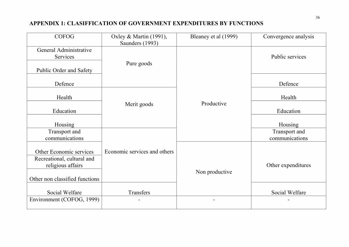
36APPENDIX 1: CLASIFFICATION OF GOVERNMENT EXPENDITURES BY FUNCTIONS

COFOG Oxley & Martin (1991), Saunders (1993)

Bleaney et al (1999) Convergence analysis

General Administrative Services

Public Order and Safety

Public services

Defence

Pure goods

Defence

Health

Health

Education

Education

Housing

Merit goods

Housing

Transport and communications

Productive

Transport and communications

Other Economic services Recreational, cultural and

religious affairs

Other non classified functions

Economic services and others

Other expenditures

Social Welfare

Transfers

Non productive

Social Welfare

Environment (COFOG, 1999) - - -

37

APPENDIX 2. RESULTS OF THE CONVERGENCE ESTIMATIONS FOR EACH FUNCTION OF THE GOVERNMENT EXPENDITURES

β CONVERGENCE IN PUBLIC SERVICES EXPENDITURE

1970-1998 1970-1979 1980-1989 1990-1997

Fixedeffects

Random effects

Fixed effects

Random effects

Fixed effects Randomeffects

Fixed effects

Random effects

β

-0.25 (-2.60)

-0.11 (-6.82)

-0.12 (-0.91)

-0.03 (-1.05)

-0.76(-2.97)

-0.15 (-5.01)

-0.63 (-2.20)

-0.13 (-4.68)

n observations 702 702 234 234 260 260 208 208

adjusted R2 0.13 0.06 0.20 0.00 0.48 0.09 0.25 0.10

Hausman Test 49,86 χ2(1) 4.61 χ2(1) 192.10 χ2(1) 29.49 χ2(1) F (αi=α) 0.98 F(25,675) Chow Test F (βt=β) σ steady-state

values 0.32 70s vs 80s 70s vs 90s 80s vs 90s

σ real values 0.23 2.19 F(1,466)

1.33 F(1,414)

0.22 F(1,440)

38

β-CONVERGENCE IN HEALTH EXPENDITURE

1970-1998 1970-1979 1980-1989 1990-1997

Fixedeffects

Random effects

Fixed effects

Random effects


Fixed effects

Random effects

β

-0.12 (-5.30)

-0.01 (-1.52)

-0.24 (-3.53)

-0.02 (-2.3)

-0.39(-4.59)

0.01 (1.18)

-0.40 (-3.56)

-0.02 (-1.94)

n observations 702 702 234 234 260 260 208 208

adjusted R2 0.13 0.00 0.33 0.02 0.38 0.01 0.32 0.02

Hausman Test 69.58 χ2(1) 32.33 χ2(1) 114.08 χ2(1) 54.86 χ2(1) F (αi=α) 3.27 F(25,675) Chow Test F (βt=β) σ steady-state


σ real values 0.32 4.5 F(1.466)

1.0 F(1,414)

1.71 F(1,440)

39

β-CONVERGENCE IN SOCIAL SECURITY EXPENDITURE

1970-1998 1970-1979 1980-1989 1990-1997

Fixedeffects

Random effects

Fixed effects

Random effects


Fixed effects

Random effects

β

-0.13 (-3.39)

-0.02 (-3.50)

-0.68 (-4.73)

-0.02 (-1.79)

-0.46(-2.97)

-0.00 (-0.29)

-0.20 (-1.00)

-0.07 (-7.43)

n observations 702 702 234 234 260 260 208 208

adjusted R2 0.07 0.02 0.295 0.01 0.38 0.00 0.31 0.21



σ real values 0.33 0.2 F(1,466)

2.4 F(1,414)

5.5 F(1,440)

40

β-CONVERGENCE IN EDUCATION EXPENDITURE

1970-1998 1970-1979 1980-1989 1990-1997

Fixedeffects

Random effects

Fixed effects

Random effects


Fixed effects

Random effects

β

-0.09 (-4.58)

-0.06 (-5.84)

-0.20 (-2.82)

-0.08 (-4.94)

-0.32(-4.75)

-0.08 (-4.11)

-0.28 (-4.32)

-0.02 (-0.89)

n observations 702 702 234 234 260 260 208 208

adjusted R2 0.13 0.04 0.33 0.10 0.26 0.06 0.31 0.00



σ real values 0.26 14.1 F(1,466)

0.3 F(1,414)

2.5 F(1,440)

41

β-CONVERGENCE IN DEFENCE EXPENDITURE

1970-1998 1970-1979 1980-1989 1990-1997

Fixedeffects

Random effects

Fixed effects

Random effects


Fixed effects

Random effects

β

-0.18 (-7.94)

-0.02 (-4.06)

-0.22 (-6.66)

-0.05 (-4.17)

-0.40(-6.96)

-0.02 (-1.51)

-0.36 (-5.32)

-0.03 (-3.05)

n observations 675 620 225 225 250 250 200 200

adjusted R2 0.17 0.02 0.58 0.04 0.31 0.01 0.36 0.04



σ real values 0.53 14,5 F(1,388)

4,3 F(1,398)

24.1 F(1,423)

42

β-CONVERGENCE IN TRANSPORT AND COMMUNICATIONS EXPENDITURE

1970-1998 1970-1979 1980-1989 1990-1997

Fixedeffects

Random effects

Fixed effects

Random effects


Fixed effects

Random effects

β

-0.16 (-4.46)

-0.36 (-3.59)

-0.35 (-3.92)

-0.05 (-2.78)

-0.27(-3.40)

-0.03 (-2.00)

-0.31 (-3.73)

-0.04 (-1.86)

n observations 702 702 234 234 260 260 208 208

adjusted R2 0.10 0.02 0.31 0.03 0.20 0.02 0.28 0.01


values 0,47 70s vs 80s 70s vs 90s 80s vs 90s

σ real values 0,60 0.82 F(1,466)

1,09 F(1,414)

0,84 F(1,440)

43

β-CONVERGENCE IN HOUSING EXPENDITURE

1970-1998 1970-1979 1980-1989 1990-1997

Fixedeffects

Random effects

Fixed effects

Random effects


Fixed effects

Random effects

β

-0.20 (-2.76)

-0.05 (-3.83)

-0.37 (-3.01)

-0.05 (-2.57)

-0.36(-4.10)

-0.05 (-2.40)

-0.43 (-2.39)

-0.05 (-1.80)

n observations 692 692 225 225 259 259 208 208

adjusted R2 0.11 0.02 0.22 0.03 0.22 0.02 0.29 0.02

Hausman Test 55.81 χ2(1) 32.63 χ2(1) 42.95 χ2(1) 54.34 χ2(1) F (αi=α) 1.15 F(25,665) Chow Test F (βt=β)

σ steady-state values

0.49 70s vs 80s 70s vs 90s 80s vs 90s

σ real values 0.52 0.12 F(1,456)

0.09 F(1,405)

0.07 F(1,439)

44

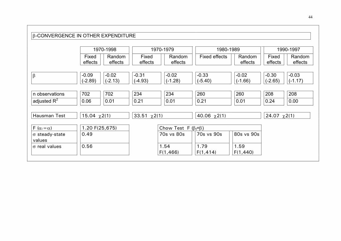
β-CONVERGENCE IN OTHER EXPENDITURE

1970-1998 1970-1979 1980-1989 1990-1997

Fixedeffects

Random effects

Fixed effects

Random effects


Fixed effects

Random effects

β

-0.09 (-2.89)

-0.02 (-2.13)

-0.31 (-4.93)

-0.02 (-1.28)

-0.33(-5.40)

-0.02 (-1.66)

-0.30 (-2.65)

-0.03 (-1.17)

n observations 702 702 234 234 260 260 208 208

adjusted R2 0.06 0.01 0.21 0.01 0.21 0.01 0.24 0.00



σ real values 0.56 1.54 F(1,466)

1.79 F(1,414)

1.59 F(1,440)

ismael sanz and francisco j. velázquez european economy group

Documents