isogeometric analysis and shape optimization in fluid...
TRANSCRIPT

Introduction Navier-Stokes Flow Shape Optimization Flow Acoustics Conclusions
Isogeometric Analysis and ShapeOptimization in Fluid Mechanics
Peter Nørtoft
DTU Compute
Joint work with Jens Gravesen, Allan R. Gersborg, Niels L. Pedersen,
Morten Willatzen, Anton Evgrafov, Dang Manh Nguyen, and Tor Dokken
Scientific Computing Section Seminar, September 17, 2013

Introduction Navier-Stokes Flow Shape Optimization Flow Acoustics Conclusions
Goals and Outline
The aim is to analyze and optimize flows using isogeometric analysis
Shape Optimization
drag
Navier-Stokes Flow Model
Isogeometric Analysis
Flow Acoustics Model
+

Introduction Navier-Stokes Flow Shape Optimization Flow Acoustics Conclusions
Goals and Outline
The aim is to analyze and optimize flows using isogeometric analysis
Shape Optimization
drag
Navier-Stokes Flow Model
Isogeometric Analysis
Flow Acoustics Model
+

Introduction Navier-Stokes Flow Shape Optimization Flow Acoustics Conclusions
Goals and Outline
The aim is to analyze and optimize flows using isogeometric analysis
Shape Optimization
drag
Navier-Stokes Flow Model
Isogeometric Analysis
Flow Acoustics Model
+

Introduction Navier-Stokes Flow Shape Optimization Flow Acoustics Conclusions
Goals and Outline
The aim is to analyze and optimize flows using isogeometric analysis
Shape Optimization
drag
Navier-Stokes Flow Model
Isogeometric Analysis
Flow Acoustics Model
+

Introduction Navier-Stokes Flow Shape Optimization Flow Acoustics Conclusions
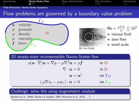
Fluid Mechanics: Navier-Stokes Equations
Flow problems are governed by a boundary value problem
ΓN
ΓD
Ω
u velocityp pressureρ densityµ viscosityf force
[M. Van Dyke]
Re = ρULµ . 103
I viscous fluid
I slow flow
I small scale
2D steady-state incompressible Navier-Stokes flow
ρ(u · ∇)u+∇p− µ∇2u = ρf in Ω
∇ · u = 0 in Ω
u = u∗ on ΓD
(µ∇ui − p ei ) · n = 0 on ΓN
Challenge: solve this using isogeometric analysis[Bazilevs et al., 2006b; Bazilevs & Hughes, 2008; Akkerman et al., 2010; . . .]

Introduction Navier-Stokes Flow Shape Optimization Flow Acoustics Conclusions
Fluid Mechanics: Navier-Stokes Equations
Flow problems are governed by a boundary value problem
ΓN
ΓD
Ω
u velocityp pressureρ densityµ viscosityf force
[M. Van Dyke]
Re = ρULµ . 103
I viscous fluid
I slow flow
I small scale
2D steady-state incompressible Navier-Stokes flow
ρ(u · ∇)u+∇p− µ∇2u = ρf in Ω
∇ · u = 0 in Ω
u = u∗ on ΓD
(µ∇ui − p ei ) · n = 0 on ΓN
Challenge: solve this using isogeometric analysis[Bazilevs et al., 2006b; Bazilevs & Hughes, 2008; Akkerman et al., 2010; . . .]

Introduction Navier-Stokes Flow Shape Optimization Flow Acoustics Conclusions
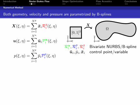
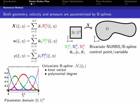
Numerical Method
Both geometry, velocity and pressure are parametrized by B-splines
X(ξ, η) =Ng∑i=1
xiRgi (ξ, η)
u(ξ, η) =Nu∑i=1
uiPui (ξ, η)
p(ξ, η) =
Np∑i=1
piPpi (ξ, η)
Ω
X
[0, 1]2y
x
η
ξ
Rui ,R
pi ,
Rgi Bivariate NURBS
/B-splineui, pi,
xi control point
/variable

Introduction Navier-Stokes Flow Shape Optimization Flow Acoustics Conclusions
Numerical Method
Both geometry, velocity and pressure are parametrized by B-splines
X(ξ, η) =
Ng∑i=1
xiRgi (ξ, η)
u(ξ, η) =Nu∑i=1
uiPui (ξ, η)
p(ξ, η) =
Np∑i=1
piPpi (ξ, η)
ΩX
[0, 1]2y
x
η
ξ
Rui ,R
pi ,
Rgi Bivariate NURBS
/B-splineui, pi,
xi control point
/variable
Introduction Navier-Stokes Flow Shape Optimization Flow Acoustics Conclusions
Numerical Method
Both geometry, velocity and pressure are parametrized by B-splines
X(ξ, η) =
Ng∑i=1
xiRgi (ξ, η)
u(ξ, η) =
Nu∑i=1
uiPui (ξ, η)
p(ξ, η) =
Np∑i=1
piPpi (ξ, η)
ΩX
[0, 1]2y
x
η
ξ
Rui ,R
pi ,R
gi Bivariate NURBS/B-spline
ui, pi, xi control point/variable
Univariate B-spline:
Ni(ξ1), Mj(ξ2)
• knot vector• polynomial degree
Parameter domain [0, 1]2
Introduction Navier-Stokes Flow Shape Optimization Flow Acoustics Conclusions
Numerical Method
Both geometry, velocity and pressure are parametrized by B-splines
X(ξ, η) =
Ng∑i=1
xiRgi (ξ, η)
u(ξ, η) =
Nu∑i=1
uiPui (ξ, η)
p(ξ, η) =
Np∑i=1
piPpi (ξ, η)
ΩX
[0, 1]2y
x
η
ξ
Rui ,R
pi ,R
gi Bivariate NURBS/B-spline
ui, pi, xi control point/variable
Univariate B-spline: Ni(ξ1)
, Mj(ξ2)
• knot vector• polynomial degree
Parameter domain [0, 1]2

Introduction Navier-Stokes Flow Shape Optimization Flow Acoustics Conclusions
Numerical Method
Both geometry, velocity and pressure are parametrized by B-splines
X(ξ, η) =
Ng∑i=1
xiRgi (ξ, η)
u(ξ, η) =
Nu∑i=1
uiPui (ξ, η)
p(ξ, η) =
Np∑i=1
piPpi (ξ, η)
ΩX
[0, 1]2y
x
η
ξ
Rui ,R
pi ,R
gi Bivariate NURBS/B-spline
ui, pi, xi control point/variable
Univariate B-spline: Ni(ξ1), Mj(ξ2)• knot vector• polynomial degree
Parameter domain [0, 1]2
Bivariate Tensor Product B-spline:• 2 knot vectors• 2 polynomial degrees• Pi,j(ξ1, ξ2) = Ni(ξ1)Mj(ξ2)
Physical domain Ω

Introduction Navier-Stokes Flow Shape Optimization Flow Acoustics Conclusions
Numerical Method
Both geometry, velocity and pressure are parametrized by B-splines
X(ξ, η) =
Ng∑i=1
xiRgi (ξ, η)
u(ξ, η) =
Nu∑i=1
uiPui (ξ, η)
p(ξ, η) =
Np∑i=1
piPpi (ξ, η)
ΩX
[0, 1]2y
x
η
ξ
Rui ,R
pi ,R
gi Bivariate NURBS/B-spline
ui, pi, xi control point/variable
Univariate B-spline: Ni(ξ1), Mj(ξ2)• knot vector• polynomial degree
Parameter domain [0, 1]2
Bivariate Tensor Product B-spline:• 2 knot vectors• 2 polynomial degrees• Pi,j(ξ1, ξ2) = Ni(ξ1)Mj(ξ2)
Physical domain ΩM(U)U = F

Introduction Navier-Stokes Flow Shape Optimization Flow Acoustics Conclusions
Error Convergence
Test of error convergence: flow with analytical solution
−3 −2 −1 0 1 2 3−1.5
−1
−0.5
0
0.5
1
1.5
x
y
−3 −2 −1 0 1 2 3−1.5
−1
−0.5
0
0.5
1
1.5
x
y
f1 = f1(x,y)
f2 = f2(x,y)
u|Γ = 0
u?1 = −U sin(πr2)y
u?2 = U/4 sin(πr2)x
p? = 4/π2 + cos(πr)
r =√
(x/2)2+ y2
u?
p?Re = 200
ε2u =∫∫Ω
‖u(x,y)−u?(x,y)‖2 dxdy

Introduction Navier-Stokes Flow Shape Optimization Flow Acoustics Conclusions
Error Convergence
Test of error convergence: flow with analytical solution
−3 −2 −1 0 1 2 3−1.5
−1
−0.5
0
0.5
1
1.5
x
y
−3 −2 −1 0 1 2 3−1.5
−1
−0.5
0
0.5
1
1.5
x
y
f1 = f1(x,y)
f2 = f2(x,y)
u|Γ = 0
u?1 = −U sin(πr2)y
u?2 = U/4 sin(πr2)x
p? = 4/π2 + cos(πr)
r =√
(x/2)2+ y2
u?
p?
Re = 200
ε2u =∫∫Ω
‖u(x,y)−u?(x,y)‖2 dxdy

Introduction Navier-Stokes Flow Shape Optimization Flow Acoustics Conclusions
Error Convergence
Test of error convergence: flow with analytical solution
−3 −2 −1 0 1 2 3−1.5
−1
−0.5
0
0.5
1
1.5
x
y
−3 −2 −1 0 1 2 3−1.5
−1
−0.5
0
0.5
1
1.5
x
y
f1 = f1(x,y)
f2 = f2(x,y)
u|Γ = 0
u?1 = −U sin(πr2)y
u?2 = U/4 sin(πr2)x
p? = 4/π2 + cos(πr)
r =√
(x/2)2+ y2
u?
p?Re = 200
ε2u =∫∫Ω
‖u(x,y)−u?(x,y)‖2 dxdy

Introduction Navier-Stokes Flow Shape Optimization Flow Acoustics Conclusions
Error Convergence
Test of error convergence: flow with analytical solution
−3 −2 −1 0 1 2 3−1.5
−1
−0.5
0
0.5
1
1.5
x
y
−3 −2 −1 0 1 2 3−1.5
−1
−0.5
0
0.5
1
1.5
x
y
f1 = f1(x,y)
f2 = f2(x,y)
u|Γ = 0
u?1 = −U sin(πr2)y
u?2 = U/4 sin(πr2)x
p? = 4/π2 + cos(πr)
r =√
(x/2)2+ y2
u?
p?Re = 200
ε2u =∫∫Ω
‖u(x,y)−u?(x,y)‖2 dxdy

Introduction Navier-Stokes Flow Shape Optimization Flow Acoustics Conclusions
Error Convergence
Discretizations with higher regularity perform better
10−5
100
εu
102
103
104
105
10−5
100
εp
Nvar
10−6
10−4
10−2
100
102
ε∇ u
102
103
104
10510
−6
10−4
10−2
100
102
ε∇ p
Nvar
u4114
11 v4
114
11 p4
014
01
u4024
02 v4
024
02 p4
014
01
u4114
11 v4
114
11 p3
013
01
u4024
02 v4
024
02 p3
013
01
u4114
11 v4
114
11 p2
012
01
u4024
02 v4
024
02 p2
012
01
u4014
01 v4
014
01 p2
012
01
u4114
12 v4
124
11 p3
013
01
u4113
11 v3
114
11 p3
013
01
DOF102 103 104 105
1
2
Smoothness Mesh Density
Strategy 1 High High
Strategy 2 Low Low
10−5
100
εu
102
103
104
105
10−5
100
εp
Nvar
10−6
10−4
10−2
100
102
ε∇ u
102
103
104
10510
−6
10−4
10−2
100
102
ε∇ p
Nvar
u4114
11 v4
114
11 p4
014
01
u4024
02 v4
024
02 p4
014
01
u4114
11 v4
114
11 p3
013
01
u4024
02 v4
024
02 p3
013
01
u4114
11 v4
114
11 p2
012
01
u4024
02 v4
024
02 p2
012
01
u4014
01 v4
014
01 p2
012
01
u4114
12 v4
124
11 p3
013
01
u4113
11 v3
114
11 p3
013
01
a
b
c
d
e
f
g
h
i
1
2
1
2
1
2
1
2

Introduction Navier-Stokes Flow Shape Optimization Flow Acoustics Conclusions
Design of Minimal Drag Body
We design a body with minimal drag
Aim
Design boundary γ of body with
area A0 travelling at constant speed
U to minimize the drag D
Optimization Problem
minγ(xb)
c = D + εR
s. t. Area ≥ A0
L−(xb) ≤ L(xb) ≤ L+(xb)
MU = F
dragobjective
areaconstraint
lineardesignconstraints
governingequations
D =∫γ
(− pI + µ
(∇u + (∇u)T
))n ds · eu
[Pironneau, 1973; 1974; Mohammadi & Pironneau, 2010]
D
γ
A0U
γ
u = 0
-r
u = Ue1
v = ∂u/∂n = 0
ΓN
20r
20r 40r
6
?--

Introduction Navier-Stokes Flow Shape Optimization Flow Acoustics Conclusions
Design of Minimal Drag Body
We design a body with minimal drag
Aim
Design boundary γ of body with
area A0 travelling at constant speed
U to minimize the drag D
Optimization Problem
minγ(xb)
c = D + εR
s. t. Area ≥ A0
L−(xb) ≤ L(xb) ≤ L+(xb)
MU = F
dragobjective
areaconstraint
lineardesignconstraints
governingequations
D =∫γ
(− pI + µ
(∇u + (∇u)T
))n ds · eu
[Pironneau, 1973; 1974; Mohammadi & Pironneau, 2010]
D
γ
A0U
γu = 0
-r
u = Ue1
v = ∂u/∂n = 0
ΓN
20r
20r 40r
6
?--

Introduction Navier-Stokes Flow Shape Optimization Flow Acoustics Conclusions
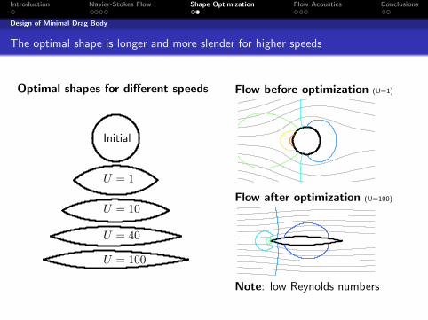
Design of Minimal Drag Body
The optimal shape is longer and more slender for higher speeds
Optimal shapes for different speeds
Initial
U = 1
U = 10
U = 40
U = 100
Flow before optimization (U=1)
Flow after optimization (U=100)
Note: low Reynolds numbers

Introduction Navier-Stokes Flow Shape Optimization Flow Acoustics Conclusions
Design of Minimal Drag Body
The optimal shape is longer and more slender for higher speeds
Optimal shapes for different speeds
Initial
U = 1
U = 10
U = 40
U = 100
Flow before optimization (U=1)
Flow after optimization (U=100)
Note: low Reynolds numbers

Introduction Navier-Stokes Flow Shape Optimization Flow Acoustics Conclusions
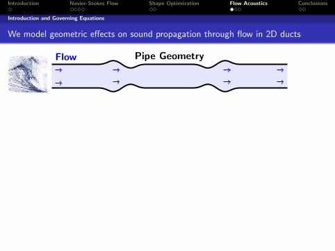
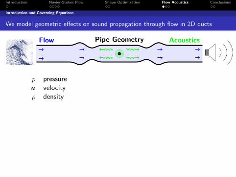
Introduction and Governing Equations
We model geometric effects on sound propagation through flow in 2D ducts
Pipe Geometry
Flow Acoustics
p pressureu velocityρ density
ρ∂u
∂t+ ρ(u · ∇)u+∇p− µ∇2u = 0
∂ρ
∂t+∇ · (ρu) = 0
p = p0 + p′
u = u0 + u′
ρ = ρ0 + ρ′
Background Flow: p0, u0, ρ0
Acoustic Disturbance: p′, u′, ρ′
1
2
⇓
γ− γ+
Γw
Γs
Ω
Introduction Navier-Stokes Flow Shape Optimization Flow Acoustics Conclusions
Introduction and Governing Equations
We model geometric effects on sound propagation through flow in 2D ducts
Pipe GeometryFlow
Acoustics
p pressureu velocityρ density
ρ∂u
∂t+ ρ(u · ∇)u+∇p− µ∇2u = 0
∂ρ
∂t+∇ · (ρu) = 0
p = p0 + p′
u = u0 + u′
ρ = ρ0 + ρ′
Background Flow: p0, u0, ρ0
Acoustic Disturbance: p′, u′, ρ′
1
2
⇓
γ− γ+
Γw
Γs
Ω

Introduction Navier-Stokes Flow Shape Optimization Flow Acoustics Conclusions
Introduction and Governing Equations
We model geometric effects on sound propagation through flow in 2D ducts
Pipe GeometryFlow Acoustics
p pressureu velocityρ density
ρ∂u
∂t+ ρ(u · ∇)u+∇p− µ∇2u = 0
∂ρ
∂t+∇ · (ρu) = 0
p = p0 + p′
u = u0 + u′
ρ = ρ0 + ρ′
Background Flow: p0, u0, ρ0
Acoustic Disturbance: p′, u′, ρ′
1
2
⇓
γ− γ+
Γw
Γs
Ω

Introduction Navier-Stokes Flow Shape Optimization Flow Acoustics Conclusions
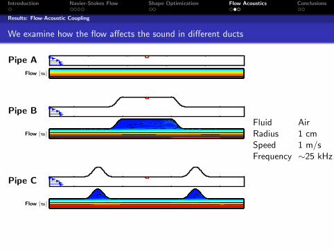
Results: Flow-Acoustic Coupling
We examine how the flow affects the sound in different ducts
-----Pipe A
|u|Flow
|p|Sound
-----Pipe B
|u|Flow
|p|Sound
-----Pipe C
|u|Flow
|p|Sound
FluidRadiusSpeedFrequency
Air1 cm1 m/s∼25 kHz
Introduction Navier-Stokes Flow Shape Optimization Flow Acoustics Conclusions
Results: Flow-Acoustic Coupling
We examine how the flow affects the sound in different ducts
-----Pipe A
|u|Flow
|p|Sound
-----Pipe B
|u|Flow
|p|Sound
-----Pipe C
|u|Flow
|p|Sound
FluidRadiusSpeedFrequency
Air1 cm1 m/s∼25 kHz
Introduction Navier-Stokes Flow Shape Optimization Flow Acoustics Conclusions
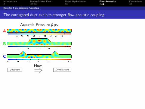
Results: Flow-Acoustic Coupling
The corrugated duct exhibits stronger flow-acoustic coupling
Acoustic Pressure p [Pa]
A
B
C
FlowUpstream Downstream⇒
Measure of Flow-Acoustic Coupling
〈δp〉 =
∫∫Ω |p(x)− p(−x)| dA∫∫
Ω |p(x)|dA
Sound Frequency Sensitivity
20 21 22 23 24 25 26 27 28 29 300
5
10
15
20 0
0.2
0.4
0.6
0.8
Pipe A
Pipe B
Pipe C
•
〈δp〉
f [kHz]
2520 30
Flow Speed Sensitivity
0 0.1 0.2 0.3 0.4 0.5 0.6 0.7 0.8 0.9 10
0.1
0.2
0.3
0.4
0.5
0.6
0.7
0.8
Pipe A
Pipe B
Pipe C
〈δp〉
U0 [m s−1]

Introduction Navier-Stokes Flow Shape Optimization Flow Acoustics Conclusions
Outlook
Ongoing work
Flow Discretizations using Locally Refinable B-splines
1 2
Optimization of Parametrizations for Isogeometric Analysis
L(U) = 0
Ω
Γ
?
?
minimize c(Ω, U)
such that det(J) > 0
where ∂Ω = Γ
L(U) = 0

Introduction Navier-Stokes Flow Shape Optimization Flow Acoustics Conclusions
Outlook
Ongoing work
Flow Discretizations using Locally Refinable B-splines
Region of Interest
Computational Domain
1 2
Optimization of Parametrizations for Isogeometric Analysis
L(U) = 0
Ω
Γ
?
?
minimize c(Ω, U)
such that det(J) > 0
where ∂Ω = Γ
L(U) = 0

Introduction Navier-Stokes Flow Shape Optimization Flow Acoustics Conclusions
Outlook
Ongoing work
Flow Discretizations using Locally Refinable B-splines
Region of Interest
Global Refinement
1 2
Optimization of Parametrizations for Isogeometric Analysis
L(U) = 0
Ω
Γ
?
?
minimize c(Ω, U)
such that det(J) > 0
where ∂Ω = Γ
L(U) = 0

Introduction Navier-Stokes Flow Shape Optimization Flow Acoustics Conclusions
Outlook
Ongoing work
Flow Discretizations using Locally Refinable B-splines
Region of Interest
Local Refinement
1 2
Optimization of Parametrizations for Isogeometric Analysis
L(U) = 0
Ω
Γ
?
?
minimize c(Ω, U)
such that det(J) > 0
where ∂Ω = Γ
L(U) = 0

Introduction Navier-Stokes Flow Shape Optimization Flow Acoustics Conclusions
Outlook
Ongoing work
Flow Discretizations using Locally Refinable B-splines
Region of Interest
Local Refinement1
2
Optimization of Parametrizations for Isogeometric Analysis
L(U) = 0
Ω
Γ
?
?
minimize c(Ω, U)
such that det(J) > 0
where ∂Ω = Γ
L(U) = 0

Introduction Navier-Stokes Flow Shape Optimization Flow Acoustics Conclusions
Outlook
Ongoing work
Flow Discretizations using Locally Refinable B-splines
Region of Interest
Local Refinement1 2
Optimization of Parametrizations for Isogeometric Analysis
L(U) = 0
Ω
Γ
?
?
minimize c(Ω, U)
such that det(J) > 0
where ∂Ω = Γ
L(U) = 0

Introduction Navier-Stokes Flow Shape Optimization Flow Acoustics Conclusions
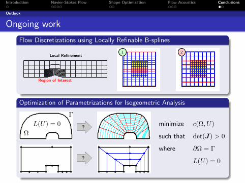
Outlook
Ongoing work
Flow Discretizations using Locally Refinable B-splines
Region of Interest
Local Refinement1 2
Optimization of Parametrizations for Isogeometric Analysis
L(U) = 0
Ω
Γ
?
?
minimize c(Ω, U)
such that det(J) > 0
where ∂Ω = Γ
L(U) = 0

Introduction Navier-Stokes Flow Shape Optimization Flow Acoustics Conclusions
Summary
Summary
Isogeometric Method
IGA = FEM (high regularity) + CAD (exact geometry)
Isogeometric Analysis of Flows
Facilitates High-regularity discretizations of flow variables
Isogeometric Shape Optimization of Flows
Unites design and analysis models through B-splines
Isogeometric Analysis of Flow Acoustics
Identifies geometric enhancement of flow-acoustic coupling

Introduction Navier-Stokes Flow Shape Optimization Flow Acoustics Conclusions
The 3 minute version: http://www.dr.dk/da
Thank You For Your Attention!