22

Color Filter Arrays: A Design MethodologyISSN 1470-5559

RR-08-03 May 2008 Department of Computer Science

Yan Li, Pengwei Hao, and Zhouchen Lin

Color Filter Arrays: A Design Methodology

Yan Li∗, Pengwei Hao†, and Zhouchen Lin‡

Abstract

In the companion report [14], we have shown that a full color im-age sampled with a rectangular color filter array (CFA) is equivalent tothe frequency domain multiplexing of multiplex components: a luminancecomponent (luma) at the baseband and several chrominance components(chromas) at high frequency bands. A matrix, called the frequency struc-ture of a CFA, is defined to represent this modulation, with which we caneasily analyze the characteristics of CFAs. The frequency structure can becomputed by applying the symbolic discrete Fourier transform (DFT) tothe CFA pattern. In this paper, we present a CFA design methodology inthe frequency domain. In this methodology, a good frequency structureof the CFA is first selected, mainly according to the following criteria:(i). the number of nonzero chromas should be as small as possible; (ii).the distance between nonzero multiplex components should be as largeas possible; and (iii). dependent (e.g., identical, negative, or conjugate)chromas should be as many as possible; and then the optimal primaryCFA patterns are computed by minimizing the norm of the demosaickingmatrix under constraints that: (i). the primary CFA patterns are all realand nonnegative; and (ii). their sum is an all-one matrix. The constraintscan be determined by applying the inverse symbolic DFT to the specifiedfrequency structure. Finally, the desired CFA pattern is the symbolic sumof the optimal primary CFA patterns. Using our methodology, a series ofnew CFA patterns are found which outperform the currently commercial-ized and published ones. Experiments demonstrate the effectiveness of ourCFA design methodology and the superiority of our new CFA patterns.

Keywords: color filter array (CFA), discrete Fourier transform (DFT),sampling, multiplexing, demosaicking

∗Y. Li is with the State Key Laboratory of Machine Perception, Peking University, Beijing100871, China (e-mail: yanli8083@gmail.com).

†P. Hao is with the Department of Computer Science, Queen Mary, University of London,London E1 4NS, U.K.,(e-mail: phao@dcs.qmul.ac.uk).

‡Z. Lin is with Microsoft Research Asia, 5th Floor, Sigma Building, Zhichun Road 49#,Haidian District, Beijing 100080, China (e-mail: zhoulin@microsoft.com).

1

1 Introduction

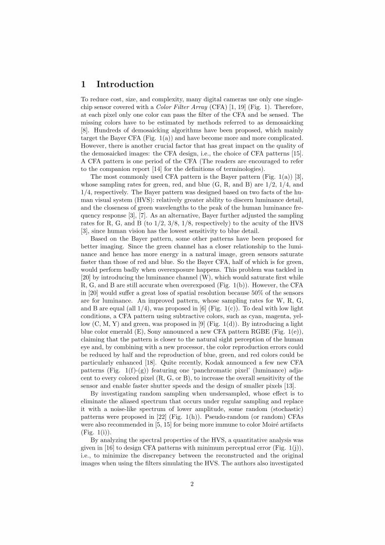
To reduce cost, size, and complexity, many digital cameras use only one single-chip sensor covered with a Color Filter Array (CFA) [1, 19] (Fig. 1). Therefore,at each pixel only one color can pass the filter of the CFA and be sensed. Themissing colors have to be estimated by methods referred to as demosaicking[8]. Hundreds of demosaicking algorithms have been proposed, which mainlytarget the Bayer CFA (Fig. 1(a)) and have become more and more complicated.However, there is another crucial factor that has great impact on the quality ofthe demosaicked images: the CFA design, i.e., the choice of CFA patterns [15].A CFA pattern is one period of the CFA (The readers are encouraged to referto the companion report [14] for the definitions of terminologies).

The most commonly used CFA pattern is the Bayer pattern (Fig. 1(a)) [3],whose sampling rates for green, red, and blue (G, R, and B) are 1/2, 1/4, and1/4, respectively. The Bayer pattern was designed based on two facts of the hu-man visual system (HVS): relatively greater ability to discern luminance detail,and the closeness of green wavelengths to the peak of the human luminance fre-quency response [3], [7]. As an alternative, Bayer further adjusted the samplingrates for R, G, and B (to 1/2, 3/8, 1/8, respectively) to the acuity of the HVS[3], since human vision has the lowest sensitivity to blue detail.

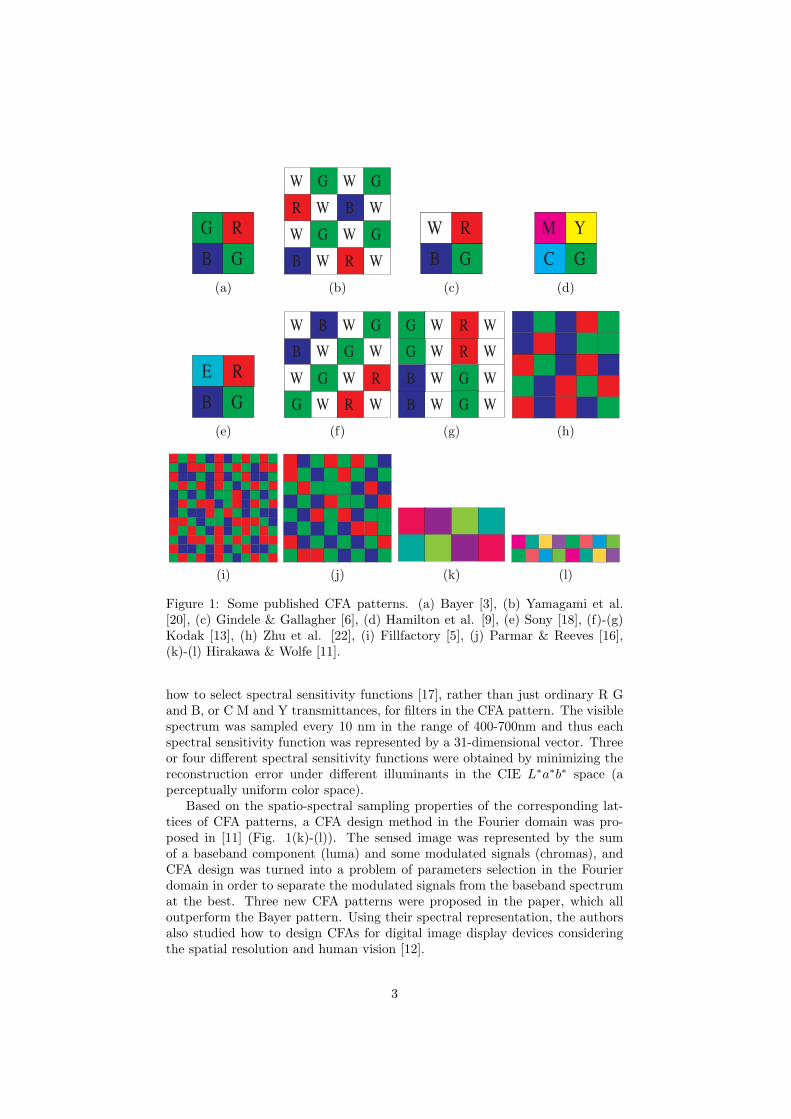
Based on the Bayer pattern, some other patterns have been proposed forbetter imaging. Since the green channel has a closer relationship to the lumi-nance and hence has more energy in a natural image, green sensors saturatefaster than those of red and blue. So the Bayer CFA, half of which is for green,would perform badly when overexposure happens. This problem was tackled in[20] by introducing the luminance channel (W), which would saturate first whileR, G, and B are still accurate when overexposed (Fig. 1(b)). However, the CFAin [20] would suffer a great loss of spatial resolution because 50% of the sensorsare for luminance. An improved pattern, whose sampling rates for W, R, G,and B are equal (all 1/4), was proposed in [6] (Fig. 1(c)). To deal with low lightconditions, a CFA pattern using subtractive colors, such as cyan, magenta, yel-low (C, M, Y) and green, was proposed in [9] (Fig. 1(d)). By introducing a lightblue color emerald (E), Sony announced a new CFA pattern RGBE (Fig. 1(e)),claiming that the pattern is closer to the natural sight perception of the humaneye and, by combining with a new processor, the color reproduction errors couldbe reduced by half and the reproduction of blue, green, and red colors could beparticularly enhanced [18]. Quite recently, Kodak announced a few new CFApatterns (Fig. 1(f)-(g)) featuring one ‘panchromatic pixel’ (luminance) adja-cent to every colored pixel (R, G, or B), to increase the overall sensitivity of thesensor and enable faster shutter speeds and the design of smaller pixels [13].

By investigating random sampling when undersampled, whose effect is toeliminate the aliased spectrum that occurs under regular sampling and replaceit with a noise-like spectrum of lower amplitude, some random (stochastic)patterns were proposed in [22] (Fig. 1(h)). Pseudo-random (or random) CFAswere also recommended in [5, 15] for being more immune to color Moire artifacts(Fig. 1(i)).

By analyzing the spectral properties of the HVS, a quantitative analysis wasgiven in [16] to design CFA patterns with minimum perceptual error (Fig. 1(j)),i.e., to minimize the discrepancy between the reconstructed and the originalimages when using the filters simulating the HVS. The authors also investigated

2

G B

R G

(a)

W G

W W W W

W W W

G G

G R

R

B

B (b)

G B R W

(c)

G C Y M

(d)

E B

R G

(e)

G B

R W W

W W

W W W

W G

G G

B

R (f)

G

B

R W

W

W W W

W W W G

G

G B

R

(g) (h)

(i) (j) (k) (l)

Figure 1: Some published CFA patterns. (a) Bayer [3], (b) Yamagami et al.[20], (c) Gindele & Gallagher [6], (d) Hamilton et al. [9], (e) Sony [18], (f)-(g)Kodak [13], (h) Zhu et al. [22], (i) Fillfactory [5], (j) Parmar & Reeves [16],(k)-(l) Hirakawa & Wolfe [11].

how to select spectral sensitivity functions [17], rather than just ordinary R Gand B, or C M and Y transmittances, for filters in the CFA pattern. The visiblespectrum was sampled every 10 nm in the range of 400-700nm and thus eachspectral sensitivity function was represented by a 31-dimensional vector. Threeor four different spectral sensitivity functions were obtained by minimizing thereconstruction error under different illuminants in the CIE L∗a∗b∗ space (aperceptually uniform color space).

Based on the spatio-spectral sampling properties of the corresponding lat-tices of CFA patterns, a CFA design method in the Fourier domain was pro-posed in [11] (Fig. 1(k)-(l)). The sensed image was represented by the sumof a baseband component (luma) and some modulated signals (chromas), andCFA design was turned into a problem of parameters selection in the Fourierdomain in order to separate the modulated signals from the baseband spectrumat the best. Three new CFA patterns were proposed in the paper, which alloutperform the Bayer pattern. Using their spectral representation, the authorsalso studied how to design CFAs for digital image display devices consideringthe spatial resolution and human vision [12].

3

In this paper, we propose a systematic CFA design methodology. Althoughboth our methodology and that in [11] are based on analysis in the frequencydomain, our framework drastically differs from that in [11] because:

1. The objective in [11] is to separate the luma and chromas as far as possible,while ours is to recover the spectra of the primary color channels (e.g., R,G, and B) of the original image as accurately as possible. So we wouldallow identical (or negative, or conjugate) chromas coexist in order toestimate the chromas more robustly, rather than simply minimizing thenumber of chromas.

2. To achieve our goal, we propose much more criteria that a good CFAshould obey, rather than only making the multiplex components as farfrom each other as possible.

3. And we also require the norm of the demosaicking matrix (the inverse ofthe multiplexing matrix) to be minimized such that the errors in estimat-ing the luma and chromas are less amplified when they are transformedback to the spectra of the primary color channels.

Moreover, our methodology is better established on a theoretical foundation. Wehave proposed using a matrix, called the frequency structure, as a representationof a CFA pattern [14]. It records all the multiplexing information and is visuallyintuitive for qualitatively analyzing the properties of the CFA pattern. Whilein [11], only the form of the Fourier transform of images sampled with a CFAwas given, whose parameters are unknown and thus makes it difficult to analyzea CFA. In addition, with our well established theory, the formulation of findingthe optimal CFA pattern given the frequency structure and the subsequentcomputation method are straightforward. In contrast, the method in [11] forselecting optimal parameters to satisfy some given design criteria was unclear.

This paper is organized as follows. In Section 2, we propose CFA designprinciples aiming at minimizing the demosaicking error, i.e., to estimate themultiplex components as accurate as possible and to minimize the error prop-agation when the multiplex components are transformed back to the primarycolor spectra. The realization of these principles via frequency structure cus-tomization and demosaicking matrix norm minimization is elaborated in Section3 and 4, respectively. Section 5 gives a simple design example in detail, and alsoproposes some new CFA patterns. Experimental results and comparisons be-tween the Bayer CFA, the three CFAs proposed in [11], and our newly proposedones are presented in Section 6. Finally, we conclude our paper in Section 7.

2 CFA Design Principles

We believe that a good CFA should minimize the demosaicking error. In thefrequency domain, a good CFA should enable good recovery of the spectra ofthe primary color channels of the original image. In the companion report[14], we have shown that the spectrum of a CFA-filtered image is the mixtureof multiplex components centered (or modulated) at certain frequency points,where each multiplex component is further a mixture of the spectra of theprimary color channels of the original image. All these can be convenientlyrepresented by the frequency structure of the CFA. Therefore, we can estimate

4

each multiplex component first and then transform them back to the spectraof the primary color channels. We call this method the universal demosaickingalgorithm. So it becomes clear that in order to minimize the demosaickingerror, we should estimate the multiplex components as accurately as possible,and make the transform as stable as possible in order to less amplify the error inthe multiplex components. These are the principles that guide our CFA design.In the following, we give more details.

2.1 Frequency structure of CFA

The frequency structure is a visually intuitive representation of a CFA. It is amatrix S with each entry being defined as:

S(kx, ky) =∑

CH(C)

p

(kx

nx,ky

ny

)· F (C)(ωx,ωy),

kx = 0, 1, · · · , nx − 1,ky = 0, 1, · · · , ny − 1.

(1)

where C = R, G, and B, (or other primary colors), H(C)p is the DFT of the pri-

mary CFA pattern h(C)p for the color channel C, F (C) is the DFT of the C compo-

nent image f (C), and (nx, ny) is the size of the CFA pattern hp. Eq. (1) meansthat at frequencies

(kxnx

, ky

ny

)there are spectral components

∑C H(C)

p

(kxnx

, ky

ny

)·

F (C)(ωx,ωy) centering there, respectively. The spectrum of the CFA-filteredimage is exactly the multiplexing of these spectral components by modulatingthem to their corresponding frequencies. For this reason, we call each entry ofthe frequency structure the multiplex component. We also call the multiplexcomponent at the baseband (S(0, 0)) the luma and the others the chromas.

Although the definition of the frequency structure looks complex, Theorem1 of [14] shows that it can be conveniently and directly obtained by computingthe symbolic DFT of the CFA pattern hp:

SCFA = DFT [hp] , (2)

if F (C) in (1) is replaced with C symbolically.For example, the frequency structure of the commonly used Bayer pattern

(Fig. 1(a)) [3] is

SBayer = DFT

[G RB G

]=

[FL FC2

−FC2 FC1

], (3)

where

FL

FC1

FC2

= TBayer ·

RGB

with (4)

TBayer =14

1 2 1−1 2 −1−1 0 1

. (5)

SBayer shows that the spectrum of any image sampled with the Bayer CFA hasa luma FL at the baseband, and three chromas FC1, FC2, and −FC2 modulated

5

at frequencies (1/2, 1/2), (1/2, 0), and (0, 1/2), respectively. The matrix T in(4) that relates the multiplex components and the spectra of primary colors iscalled the multiplexing matrix.

2.2 Universal demosaicking and CFA design principles

With the frequency structure SCFA (2) of a CFA, demosaicking for any rect-angular CFA can be easily done in the frequency domain. Namely, we firstestimate the nonzero multiplex components, FL, FC1, and FC2, etc., from thespectrum of the CFA-filtered image using band-pass filters, then obtain thespectra of primary color component images by inverting the linear system like(4), and finally apply IDFT to the spectra of the primary color componentsto recover the full color image. This is a universal demosaicking method, andthe algorithm proposed in [4] is just this method applied to the Bayer CFA.However, its performance depends on the characteristics of the CFA. Simple asit is, we will show that with properly chosen CFA, we can still achieve superiordemosaicking results.

The inversion of the linear system like (4) induces a matrix D as the inverseof the multiplexing matrix T . We shall call this matrix D the demosaickingmatrix. For example, for the Bayer pattern, the demosaicking matrix is

DBayer = T−1Bayer =

1 −1 −21 1 01 −1 2

. (6)

It is easy to see that for the universal demosaicking method to perform well,the CFA should enable the following procedures to work well:

1. to estimate the multiplex components accurately;

2. to estimate the spectra of primary color components from the multiplexcomponents accurately.

To achieve the first goal, we have two principles:

(P1) The crosstalk among the multiplex components should be aslittle as possible.

(P2) The correlations among the multiplex components should beas high as possible.

With the first principle, band-pass filtering will result in little aliasing frequen-cies from other multiplex components. And by the second principle, we canrobustly estimate the multiplex components by taking advantage of the corre-lation among them.

To achieve the second goal, we have to control the error in the estimatedmultiplex components such that it will be less amplified. Noticing the linearrelationship between the multiplex components and the spectra of primary colorcomponents, this can be realized by minimizing the norm of the demosaickingmatrix D. Hence we have the third principle:

(P3) The norm of the demosaicking matrix D should be minimized.

6

Figure 2: All possible positions of multiplex components of the sensed image bya CFA pattern of size 3× 3.

Our CFA design methodology is based on these three principles. It consists oftwo steps: choosing an appropriate frequency structure of the CFA and choosingoptimal primary CFA patterns such that the norm of D is minimized. Thedetails are described in the following sections.

3 Choosing a CFA Frequency Structure

This section focuses on how to choose an appropriate frequency structure ofthe CFA in order to follow (P1) and (P2) in the previous section, i.e., specifythe positions of nonzero multiplex components and designate the relationship(equal, negative, or conjugate) among the chromas.

3.1 Conditions: hard constraints

The specification of frequency structure is not arbitrary. First, the centers ofthe nonzero multiplex components can only be at the lattice (kx/nx, ky/ny),kx = 0, 1, · · · , nx − 1; ky = 0, 1, · · · , ny − 1 [14]. So we can only choose amongthese points as the centers of nonzero multiplex components. Fig. 2 showsall possible centers of multiplex components when nx = ny = 3. Second, theluma must exist. So the frequency point (0, 0) must be selected by default.Third, in order to make the designed CFA pattern real, once a frequency point(kx/nx, ky/ny) in the lattice is chosen, the one (1− kx/nx, 1− ky/ny) at itsconjugate position must also be chosen. Note that the chroma at the conjugateposition, which we call the conjugate chroma, must also be symbolically conju-gate in value, i.e., the coefficients of R, G, and B channels are all conjugate tothose of the chosen chroma. These two aspects of conjugate constraints can beconveniently automated by the computer. Fourth, to reconstruct three primarycolor components of an image, we need at least three independent multiplexcomponents. Since the luma is already selected, two independent chromas mustbe selected. Here, that two chromas S(p, q) and S(r, s) are independent meansthat there does not exist a scalar (real or complex) c such that S(p, q) = c·S(r, s).If two independent chromas are chosen, the multiplexing matrix T will be ofrank 3 so that the spectra of three primary colors can be determined. This

7

independence can also be automatically checked by the computer via symboliccomputation.

Assisted by the computer, we can click on the frequency lattice to choosenonzero multiplex components. However, in order to design a good frequencystructure, we have to follow some guidelines.

3.2 Guidelines: soft constraints

To apply (P1), we may first

(G1) choose as few nonzero chromas as possible; and

(G2) maximize the distance among the nonzero multiplex compo-nents.

Moreover, due to the fact that the spectra of multiplex components havelong tails along the horizontal and the vertical axes and the energy of luma ismuch higher than those of chromas [14], which implies that the aliasing alongthe axes are the most severe, we may further wish that

(G3) the distance between luma and chromas should be large enough(e.g., no less than 0.5); and

(G4) the chromas should not be centered on the horizontal or ver-tical axes of the luma.

We can only wish (G3) and (G4) because they may not always be satisfied if thesize of the CFA pattern is too small, due to the hard constraints in Section 3.1.For example, for CFA patterns of size 3×3 (Fig. 3(b)), (G3) cannot be satisfied,and for CFA patterns of size 2× 2 (Fig. 3(a)), (G4) cannot be satisfied.

To apply (P2), we may

(G5) choose redundant nonzero chromas and make them dependent.

With redundant chromas, we can estimate each chroma more robustly by cross-checking with its redundant copies. In our current system, for simplicity weonly require that a chroma is equal to another one, rather than specifying ascalar between them. This is because being equal is the least likely to amplifythe error in the estimation. From the conjugate constraints in Section 3.1, oncethe relationship between two chromas is specified, the relationship between theirconjugate chromas will be automatically determined by the computer. Note that(G5) is in conflict with (G1). Therefore, we have to make a tradeoff between(G1) and (G5).

One should be reminded that our guidelines could not result in a uniquefrequency structure. We could not foresee which frequency structure is optimalif we make a tradeoff among the guidelines. We have to test the obtained CFApatterns with differently specified frequency structures using benchmark imagesto find the best one. Nonetheless, using our guidelines one can easily rule outa vast majority of bad frequency structures: s/he only has to test a limitednumber of designs, which are possibly the optimal. This already saves a lot ofeffort in CFA design.

8

(a) (b) (c) (d) (e)

(f) (g) (h) (i) (j)

Figure 3: Some examples of frequency structures generated with CFA patternsof size (a) 2× 2, (b) 3× 3, (c) 4× 4, (d) 5× 5, (e) 6× 6, (f) 4× 2, (g) 2× 4, (h)6× 2, (i) 10× 10, (j) 11× 11.

3.3 Examples of specifying the frequency structure

We show some examples of frequency structures with various sizes of CFA pat-terns in Fig. 3, whose corresponding frequency structures are shown in Table 1.By convention we put the baseband at the center, but all the DFT spectra areperiodic in both horizontal and vertical directions, so in our frequency structurerepresentation of CFAs, we take the frequency origin (0, 0) as at the top-leftcorner of the matrix.

Note that the frequency structures in Figs. 3(b), (g), and (j) only havetwo conjugate chromas. According to the last hard constraint in Section 3.1,they must be independent. This is possible when their coefficients of R, G,and B channels do not reduce to real or imaginary numbers simultaneously.For example, the chromas ((2R − G − B) + i

√3(G − B))/6 and ((2R − G −

B)− i√

3(G−B))/6 of the Diagonal stripe CFA [14] are independent. And onecan also see that some frequency structures (Figs.3(c), (i)) have more than twononzero chromas. This is because of guideline (G5).

4 Choosing Optimal Primary CFA Patterns

Once the form of the frequency structure, i.e., the size of the CFA pattern,the modulation frequencies of nonzero multiplex components, and the relation-ship among the chromas are chosen, the optimal primary CFA patterns can bedetermined by applying (P3).

As we have chosen the luma FL and independent chromas, e.g., FC1 and FC2,and have specified the relationship among them, the entries in the frequencystructure becomes:

S(0, 0) = FL, andS(kx, ky) ∈ {0, FC1, FC2, F ∗

C1, F∗C2}, (kx, ky) %= (0, 0),

in which ∗ means symbolic conjugate. The multiplex components are related to

9

Table 1: Frequency structures of the CFA patterns shown in Fig. 3.

»

FL FC1

0 FC2

–

2

4

FL 0 0

0 FC1 0

0 0 F ∗

C1

3

5

2

6

4

FL 0 0 0

0 0 FC2 0

0 FC3 FC1 F ∗

C3

0 0 F ∗

C20

3

7

5

2

6

6

6

4

FL 0 0 0 0

0 0 FC1 0 0

0 0 0 0 FC2

0 F ∗

C20 0 0

0 0 0 F ∗

C10

3

7

7

7

5

(a) (b) (c) (d)

2

6

6

6

6

6

4

FL 0 0 0 0 0

0 0 0 FC1 0 0

0 0 0 0 0 0

0 FC2 0 0 0 F ∗

C2

0 0 0 0 0 0

0 0 0 F ∗

C10 0

3

7

7

7

7

7

5

2

6

4

FL 0

0 FC2

0 FC1

0 F ∗

C2

3

7

5

»

FL 0 0 0

0 FC1 0 F ∗

C1

–

2

6

6

6

6

6

4

FL 0

0 FC2

0 0

0 FC1

0 0

0 F ∗

C2

3

7

7

7

7

7

5

(e) (f) (g) (h)

2

6

6

6

6

6

6

6

6

6

6

6

6

4

FL 0 0 0 0 0 0 0 0 0

0 0 0 0 0 0 0 0 0 0

0 0 0 0 0 0 0 0 0 0

0 0 0 0 FC2 0 0 0 0 0

0 0 0 0 0 0 0 FC3 0 0

0 0 0 0 0 FC1 0 0 0 0

0 0 0 F ∗

C30 0 0 0 0 0

0 0 0 0 0 0 F ∗

C20 0 0

0 0 0 0 0 0 0 0 0 0

0 0 0 0 0 0 0 0 0 0

3

7

7

7

7

7

7

7

7

7

7

7

7

5

2

6

6

6

6

6

6

6

6

6

6

6

6

6

6

4

FL 0 0 0 0 0 0 0 0 0 0

0 0 0 0 0 0 0 0 0 0 0

0 0 0 0 0 0 0 0 0 0 0

0 0 0 0 0 0 0 0 0 0 0

0 0 0 0 0 0 0 0 0 0 0

0 0 0 0 0 0 0 FC1 0 0 0

0 0 0 0 F ∗

C10 0 0 0 0 0

0 0 0 0 0 0 0 0 0 0 0

0 0 0 0 0 0 0 0 0 0 0

0 0 0 0 0 0 0 0 0 0 0

0 0 0 0 0 0 0 0 0 0 0

3

7

7

7

7

7

7

7

7

7

7

7

7

7

7

5

(i) (j)

the spectra of primary color components via the multiplexing matrix T :

FL

FC1

FC2

= T ·

RGB

, (7)

where T can be written as

T =

a(R)

L a(G)L a(B)

L

a(R)C1 + i · b(R)

C1 a(G)C1 + i · b(G)

C1 a(B)C1 + i · b(B)

C1

a(R)C2 + i · b(R)

C2 a(G)C2 + i · b(G)

C2 a(B)C2 + i · b(B)

C2

, (8)

in which all a’s and b’s are real numbers. Note that the coefficients of R, G, andB channels for FL must be real numbers because it is self-conjugate.

After plugging the expressions of the multiplex components in the frequencystructure SCFA, using the parameters in T , and applying the inverse symbolicDFT to SCFA, we can have the expressions of primary CFA patterns writtenin the parameters in T , which are all linear functions. Therefore, if we coulddetermine the optimal T , the optimal CFA pattern with the specified frequencystructure can be obtained. Optimization based on T has several advantages.First, it is more natural as all our analysis is frequency based. Second, T hasat most 15 (actually 10, as we will see in a moment) free parameters, makingthe search space relatively small. If we optimize in the spatial domain for theoptimal primary CFA patterns directly, the number of free parameters will be2nxny, which will be much larger when nxny > 8.

The constraints on T now become apparent: the primary CFA patternsmust all be real and nonnegative and their sum is an all-one matrix [14]. If theconjugate constraints in Section 3.1 are fulfilled when specifying the frequency

10

structure, it is guaranteed that the primary CFA patterns are all real. So weneed not worry about this constraint. The nonnegativity would impose 3nxny

inequality constraints and the all-one summation would impose nxny equalitieson the parameters in T . However, the number of equality constraints can begreatly reduced if we consider them in the frequency domain. As that the sumof all primary CFA patterns being an all-one matrix is equivalent to that thesum of the first row of T is 1 and those of the remaining rows are all 0, it ismore convenient to use the latter to replace the nxny equality constraints onthe parameters of T . Considering the real and the imaginary parts separately,there are 5 such equality constraints. So the number of free parameters in T isactually at most 10. It is possible that the 5 equality constraints are still notlinearly independent, but it is harmless to keep all of them.

Now the search for the optimal T becomes the following constrained opti-mization problem:

Minimize ‖ D ‖Subject to: the (at most) 5 equality constraints and

the 3nxny inequality constraints,(9)

where D = T−1 is the demosaicking matrix and the norm can be any matrixnorm. Note that it is very tedious to write down all the inequality constraintsmanually as they involve the inverse symbolic DFT of the frequency structure,particularly when nx or ny is large. But this can be done on the computer viasymbolic computing.

Although the feasible region of the parameters is convex (intersection ofhyperspaces and half spaces), the objective function is not convex with respectto the parameters. Currently we have not developed an efficient method to findthe globally optimal solution to problem (9), and only check the corners of thefeasible region. However, we have found that the solution found in this way isalready quite satisfactory.

Note that the primary colors that we have written in the previous sectionsand [14] are actually symbolic, i.e., ‘RGB’ can be real ‘red’, ‘green’, and ‘blue’,or real ‘green’, ‘blue’, and ‘red’, etc. So after obtaining an optimal CFA patternw.r.t. the symbolic ‘RGB’, we can designate ‘R’, ‘G’, and ‘B’ as any permutationof real ‘red’, ‘green’, and ‘blue’. Which pattern performs best is determined bythe statistics of red, green, and blue colors in natural images.

5 A Design Example and New CFA Patterns

The steps of our CFA design methodology described in the previous two sectionsis summarized in Fig. 4. In the following, we give a detailed example of designinga 2×2 CFA pattern by using the proposed methodology. We also present severalnew CFA patterns designed using our method.

5.1 CFA pattern design of size 2× 2

Our example follows the steps in Fig. 4.

11

Choose nonzero chromas of the frequency structure

Specify the relationship among the chromas

Obtain the constraints in problem (9)

Find the formulation of primary

CFA patterns expressed in the parameters of T

Choose a norm for D and solve problem (9)

Obtain an optimal CFA pattern with the specified frequency

structure

Permute the primary colors to find all optimal CFA patterns

Spec

ify f

requen

cy s

truct

ure

Opti

miz

atio

n

Figure 4: The flowchart of CFA pattern design.

Step 1. We choose the frequency structure of the 2× 2 CFA pattern to be(Fig. 3(a)):

S =[

FL FC1

0 FC2

], (10)

where we specify the chroma at (0, 0.5) to be zero. Note that FC1 and FC2 areboth self-conjugate. So their coefficients must all be real. Thus the multiplexingmatrix is:

T =

a(R)

L a(G)L a(B)

L

a(R)C1 a(G)

C1 a(B)C1

a(R)C2 a(G)

C2 a(B)C2

.

Step 2. As there are no redundant chromas, there is no relationship toprescribe between FC1 and FC2.

Step 3. By applying inverse symbolic DFT to S(C), the primary CFA pat-

12

G C Y M

(a)

R C Y M

(b)

B C Y

M (c)

Figure 5: Designed CFA pattern of size 2× 2 whose primary colors are (a) [R,G, B], (b) [G, R, B] and (c) [R, B, G].

terns are found to be (C = R, G, B):

h(C)p =

[a(C)

L + a(C)C1 + a(C)

C2 a(C)L − a(C)

C1 − a(C)C2

a(C)L + a(C)

C1 − a(C)C2 a(C)

L − a(C)C1 + a(C)

C2

]. (11)

Step 4. The equality constraints are:

a(R)L + a(G)

L + a(B)L = 1,

a(R)C1 + a(G)

C1 + a(B)C1 = 0,

a(R)C2 + a(G)

C2 + a(B)C2 = 0,

(12)

which are for making the sum of primary CFA patterns an all-one matrix. Notethat now we only have 3 equality constraints because the zero sum constraintson the imaginary parts of the parameters in T are automatically fulfilled. Andthe inequality constraints are:

a(C)L + a(C)

C1 + a(C)C2 ≥ 0,

a(C)L − a(C)

C1 − a(C)C2 ≥ 0,

a(C)L + a(C)

C1 − a(C)C2 ≥ 0,

a(C)L − a(C)

C1 + a(C)C2 ≥ 0,

C = R, G, B, (13)

which are for making the entries of the primary CFA patterns (11) nonnegative.Step 5. Now we choose the 2-norm as the norm of D and solve the following

optimization problem:{

Minimize ‖ D ‖2Subject to: Eqs. (12) and (13).

(14)

Step 6. After solving problem (14), we obtain a new CFA pattern

hp =[

G R+B2

R+G2

G+B2

], (15)

which is shown in Fig. 5(a). Its frequency structure is:

S =14

[R + 2G + B G−B

0 −R + G

]. (16)

13

G C

Y

M C

Y M C

Y M

R C Y

M Y Y

(a)

C Y C Y M C Y

M G

G

C Y

C Y C Y M C Y

M G

G

C Y

C Y C Y M C Y

M G

G

C Y

(b) (c)

Figure 6: The proposed CFA patterns (a) CFA4a, (b) CFA6, (c) CFA23, andthe spectra of images ‘lighthouse’ filtered with them.

G

B C Y

M C Y M

C

Y

M Y C

C C

M (a)

C Y C Y M C Y

M G

G

C Y

(b)

Figure 7: (a) CFA4b, obtained by exchanging the red and blue color in CFA4a.(b) An equivalence of CFA6.

Step 7. Permuting R, G, and B in Eq. (15), we can totally have 6 optimalCFA patterns with the specified frequency structure (10), two of which areshown in Figs. 5(b)-(c), where the RGB corresponds to real ‘green’, ‘red’, and‘blue’, and real ‘red’, ‘blue’, and ‘green’, respectively.

5.2 New patterns: CFA4a, CFA4b, CFA6 and CFA23

Using our design methodology, we have found several new CFA patterns ofvarious sizes: CFA4a (4 × 4), CFA6 (6 × 6), and CFA23 (23 × 23). They areshown in Figs. 6 (a), (b), and (c), respectively.

14

The frequency structures of CFA4a and CFA6 are respectively:

SCFA4a =

FL 0 0 00 0 FC2 00 FC2 FC1 FC2

0 0 FC2 0

, (17)

where

FL

FC1

FC2

=18

3 3 21 1 −21 −1 0

·

RGB

, (18)

and

SCFA6 =

FL 0 0 0 0 00 0 0 FC2 0 00 0 0 0 0 00 0 0 FC1 0 00 0 0 0 0 00 0 0 FC2 0 0

, (19)

where

FL

FC1

FC2

=112

3 6 33 −2 −10 −2 2

·

RGB

. (20)

The nonzero multiplex components of CFA23 are respectively:

0.332R + 0.334G + 0.334B at the baseband,(−0.166−0.023i)R+(0.103−0.132i)G+(0.063+0.155i)B at (10/23, 10/23),

and(−0.166+0.023i)R+(0.103+0.132i)G+(0.063−0.155i)B at (−10/23,−10/23).

The spectra of the image ‘lighthouse’ filtered with CFA4a, CFA6, and CFA23are shown in the second row of Fig. 6, respectively.

If we exchange the primary colors R and B in CFA4a, we can obtain anothernew CFA, denoted as CFA4b (Fig. 7(a)). Its frequency structure is the sameas that of CFA4a but the multiplexing matrix becomes

TCFA4b =18

2 3 3−2 1 10 −1 1

. (21)

Since the columns of CFA6 pattern have three periods, the CFA6 pattern isactually equivalent to a 6× 2 pattern, as shown in Fig. 7(b).

6 Experiments

Now we test our new CFA patterns with the 24 widely-used Kodak color images[4, 8] and compare them with the Bayer pattern, and three CFAs proposed byHirakawa and Wolfe [11], denoted as HWp1 (Fig. 1(k)), HWp2, and HWp3(Fig. 1(l)).

As described previously, we apply the universal demosaicking method (Sec-tion 2) to the images sampled by the CFA patterns to be tested. For HWp1,

15

Table 2: CPSNR of demosaicking algorithms based on the Bayer CFA, threeCFAs proposed in [11], and four our newly designed CFAs. As the performanceof the Adaptive method for HWp1, HWp2, and CFA6 improves very little onits Naive counterpart, we do not list the corresponding CPSNRs due to limitedspace.

Bayer HWp1 HWp2 HWp3 CFA4a CFA4b CFA6 CFA23Img. Homo POCS Naive Adapt Naive Naive Direct Naive Adapt Naive Adapt Naive Direct

1 35.13 37.82 35.55 38.14 39.94 39.43 39.36 39.48 39.65 40.31 40.39 40.16 40.822 39.10 39.58 39.20 39.82 40.71 38.77 40.23 39.85 39.92 41.46 41.41 41.57 40.533 41.21 41.66 40.99 41.28 40.76 39.89 40.67 41.31 41.64 40.94 41.13 41.12 41.324 39.00 40.07 40.59 40.68 40.30 38.38 40.29 40.15 40.24 41.80 41.88 41.57 40.195 35.42 37.57 37.08 37.68 37.27 36.28 37.15 37.17 37.82 37.09 37.47 36.82 37.196 37.61 38.65 36.94 39.95 40.84 40.31 40.58 40.16 40.82 40.63 41.06 40.78 41.037 40.51 41.74 41.72 42.09 41.32 40.24 41.28 41.94 42.16 41.49 41.64 41.57 41.478 33.77 35.35 31.85 35.13 37.75 37.16 37.19 37.25 37.56 37.76 37.97 36.78 37.659 40.93 41.91 40.51 42.02 42.10 41.61 41.88 42.31 42.48 41.70 41.85 41.56 42.2310 40.58 42.07 41.49 42.12 42.06 41.31 42.35 41.96 42.56 42.18 42.56 42.23 42.6611 37.53 39.29 38.07 39.74 40.50 39.38 39.76 39.87 40.19 40.78 41.01 40.41 40.0912 41.68 42.68 41.11 43.10 43.12 42.22 43.27 43.55 43.81 43.81 43.94 43.55 43.8413 31.36 34.42 34.06 34.93 34.96 35.48 34.22 34.61 34.97 34.88 35.10 35.11 35.1614 35.29 35.91 35.31 35.55 35.74 33.92 35.10 35.54 35.64 35.73 35.80 35.87 34.9715 37.84 39.35 39.41 39.45 39.23 38.09 39.42 39.15 39.45 40.24 40.44 40.06 39.2216 41.47 41.87 39.74 43.78 44.29 43.94 43.80 43.80 44.35 44.10 44.42 44.47 44.4817 39.23 41.49 40.93 41.32 41.67 41.70 41.34 41.27 41.62 41.26 41.50 40.97 41.0518 34.47 37.24 36.78 37.01 36.91 36.71 36.29 36.75 36.98 36.82 36.96 37.06 36.8019 38.35 39.90 36.49 40.27 41.73 41.19 41.18 41.16 41.32 41.32 41.41 40.60 41.2620 39.03 40.69 39.75 40.15 41.48 40.93 40.86 40.88 41.18 40.74 40.93 40.28 41.1221 36.56 38.97 37.47 38.70 40.27 39.82 39.63 39.82 40.08 40.07 40.21 40.22 39.8522 36.35 37.90 36.98 37.76 38.17 37.63 38.18 38.27 38.30 38.29 38.31 38.23 38.2423 41.69 41.92 41.83 41.99 42.06 40.39 41.67 42.10 42.20 42.19 42.22 42.28 41.8524 32.97 34.67 34.32 34.66 35.44 35.27 35.26 35.03 35.34 35.28 35.42 35.37 35.38

Avg. 37.80 39.28 38.26 39.47 39.94 39.17 39.62 39.72 40.01 40.04 40.21 39.94 39.93

HWp2, CFA4a, CFA4b, and CFA6, there may be identical or dependent chromasmodulated at different frequency points. There are many methods to combinethese copies for more accurate estimation of the chromas. One method is tonaively average these copies.1 The other method is the locally adaptive weight-ing method proposed in [4], which gives larger weights to the copies with lessaliasing. The latter method respects the fact that these copies suffer differentamount of aliasing. We shall call these two methods the naive and the adap-tive method, respectively. For HWp3 and CFA23, there are only two chromas,which can only be estimated by direct band-pass filtering. Therefore, we denotethese universal demosaicking algorithms as HWp3-Direct and CFA23-Direct,respectively.

For the Bayer CFA, CFA4a, and CFA4b, the Adaptive method outperformsthe Naive method greatly, especially for the Bayer CFA (1.2 dB gain on aver-age), which is not the case for HWp1, HWp2, and CFA6 (about 0.05 dB gain onaverage). We conjecture that the reason may lie in the combination character-istics of the Adaptive method. In general, the more difference several estimateshave, the more gain we can obtain by combining the estimates. Thus, for the

1If two chromas, S(p, q) and S(r, s), are dependent, which means that there exists a scalarc such that S(p, q) = c · S(r, s) (Section 3.1), then we can average S(p, q)/c and S(r, s) for abetter estimation of S(r, s).

16

(a) (b) (c)

(d)

( g )

(e)

(i) (h)

( f )

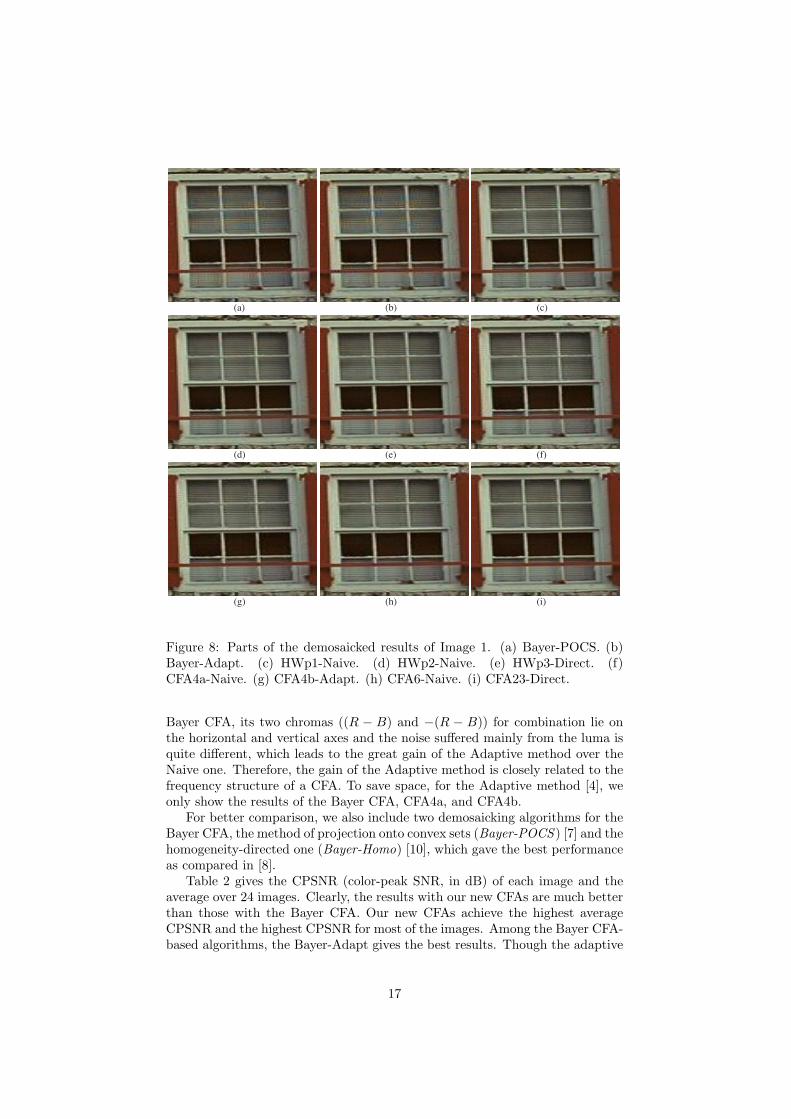
Figure 8: Parts of the demosaicked results of Image 1. (a) Bayer-POCS. (b)Bayer-Adapt. (c) HWp1-Naive. (d) HWp2-Naive. (e) HWp3-Direct. (f)CFA4a-Naive. (g) CFA4b-Adapt. (h) CFA6-Naive. (i) CFA23-Direct.

Bayer CFA, its two chromas ((R − B) and −(R − B)) for combination lie onthe horizontal and vertical axes and the noise suffered mainly from the luma isquite different, which leads to the great gain of the Adaptive method over theNaive one. Therefore, the gain of the Adaptive method is closely related to thefrequency structure of a CFA. To save space, for the Adaptive method [4], weonly show the results of the Bayer CFA, CFA4a, and CFA4b.

For better comparison, we also include two demosaicking algorithms for theBayer CFA, the method of projection onto convex sets (Bayer-POCS ) [7] and thehomogeneity-directed one (Bayer-Homo) [10], which gave the best performanceas compared in [8].

Table 2 gives the CPSNR (color-peak SNR, in dB) of each image and theaverage over 24 images. Clearly, the results with our new CFAs are much betterthan those with the Bayer CFA. Our new CFAs achieve the highest averageCPSNR and the highest CPSNR for most of the images. Among the Bayer CFA-based algorithms, the Bayer-Adapt gives the best results. Though the adaptive

17

(a) (b) (c)

(d) (e) (f)

(g) (h) (i)

Figure 9: Parts of the demosaicked results of Image 8. (a) Bayer-POCS. (b)Bayer-Adapt. (c) HWp1-Naive. (d) HWp2-Naive. (e) HWp3-Direct. (f)CFA4a-Naive. (g) CFA4b-Adapt. (h) CFA6-Naive. (i) CFA23-Direct.

technique used in Bayer-Adapt greatly improves the performance with the BayerCFA, our simple and non-adaptive CFA4a-Naive, CFA4b-Naive, CFA6-Naive,and CFA23-Direct algorithms still outperform Bayer-Adapt on average and onmost of the 24 images. This demonstrates that using our new patterns, CFA4a,CFA4b, CFA6, and CFA23, the demosaicking quality can be improved a lot.The three patterns of [11], which simply aim to improve the arrangements ofthe multiplex components, only have relatively good results. HWp1, which isthe best among them, is worse than the best (CFA4b) of our new CFA patternsand only has comparable performance with the other three of ours, in termsof average CPSNR. The other two patterns of [11], HWp2 and Hwp3, performworse than all of our new CFA patterns.

Fig. 8, 9, and 10 provide the demosaicked images for the Images 1, 8, and19. To save space, for CFA4a and CFA4b, we present only the results of CFA4a-Naive and CFA4b-Adapt, which have the worst and the best performance onaverage in terms of CPSNR, respectively, and for the Bayer pattern we presentthose of Bayer-POCS and Bayer-Adapt, which have better performance on av-erage in terms of CPSNR. The figures show that for the window of Image 1 (Fig.8) and the picket fence of Image 19 (Fig. 10), the output images of the BayerCFA have obvious artifacts even with sophisticated demosaicking algorithms,while those of our new CFAs show very few artifacts, even with simple (theNaive) algorithms. As a matter of fact, this is an inherent problem of the BayerCFA, since its spectrum has serious crosstalk along the horizontal and vertical

18

(b) (c)

(d) (e) (f)

(i) (h) (g)

(a)

Figure 10: Parts of the demosaicked results of Image 19. (a) Bayer-POCS.(b) Bayer-Adapt. (c) HWp1-Naive. (d) HWp2-Naive. (e) HWp3-Direct. (f)CFA4a-Naive. (g) CFA4b-Adapt. (h) CFA6-Naive. (i) CFA23-Direct.

axes, which can be observed from its frequency structure (for details, see theCFA analysis in [14]). Thus for images whose spectra are relatively high alongthe horizontal and vertical axes, which is usually the case for natural images[14], the Bayer CFA is doomed to perform badly. For the wires of Image 8(Fig. 9), CFA4b-Adapt outperforms others in terms of subjective quality. Asthe presence of wires corresponds to high energy in the area off the horizontaland vertical axes in the frequency space, severe aliasing may result for our newCFAs. However, by exploiting the correlations [4] among the nonzero chromas(e.g., 4 replica of (R − G)/8 for CFA4a, 4 replica of (−G + B)/8 for CFA4b,which contain different amount of aliasing), our new CFAs still perform well interms of both CPSNR (Table 2) and subjective quality. The result images ofHWp1, HWp2, and HWp3 have less obvious artifacts than those of Bayer, butstill have some. For example, the color Moire artifact on the fence support ofthe picket fence of Image 19 (Figs. 10(c)-(e)) is visible.

For the Bayer, HWp1, HWp2, and HWp3 CFAs, we have also tested theiralternative CFAs obtained by permuting the colors R, G and B, and comparedthem with our CFAs in terms of average CPSNR. For the Bayer CFA, if weexchange R and G, the average CPSNR is the highest (39.71 dB) for demo-saicking with the Adaptive method. For HWp1, its alternatives cannot lead tobetter results. As a matter of fact, the average CPSNR is 39.17 dB if G and Bexchange, and 38.88 dB if R and G exchange. For HWp2, the average CPSNRis the highest when G and B exchange (39.53 dB) but is still lower than that

19

of the Bayer CFA exchanging R and G and those of all our CFAs. For HWp3,we cannot obtain better results by permuting the color. Thus HWp1 and itsalternatives are all worse than CFA4b, and are worse than or comparable toour other CFAs. The results of Bayer, HWp2, and HWp3 CFAs and their al-ternatives are all worse than those of our proposed CFAs. This implies that theproposed methodology can find better than ever or even the best CFAs.

7 Conclusions and Future Work

Based on the frequency domain representation of CFAs, a CFA design method-ology is proposed in this paper. It aims at minimizing the demosaicking errorby better arranging multiplex components in the frequency structure and find-ing the optimal multiplexing matrix. Our experiments show that using ournew CFA patterns, the simple universal demosaicking algorithm can achieveexcellent demosaicking quality.

The performance of the universal demosaicking algorithm can be furtherimproved if better methods for combining the duplicated chromas could befound. And a fast method to find the globally optimal solution to (9) is alsodesirable. These are two of our future work. And actually the different chromasshould not be limited to two (e.g., we can specify conjugate relationship amongthe chromas to have frequency structures like that of Kodak in Table 1 of [14])such that the multiplexing matrix is of size K × 3, where K > 3. In this case,how to accurately estimate these chromas and the spectra of primary colorcomponents is also worth exploring.

References

[1] J. Adams, K. Parulski, and K. Spaulding. Color processing in digital cam-eras. IEEE Micro, vol. 18, no. 6, pp. 20-31, 1998.

[2] D. Alleysson, S. Susstrunk, and J. Herault. Linear demosaicing inspired bythe human visual system. IEEE Trans. Image Process., 14(4):439-449, 2005.

[3] B.E. Bayer. Color imaging array. U.S. Patent 3 971 065, 1976.

[4] E. Dubois. Frequency-domain methods for demosaicking of Bayer-sampledcolor images. IEEE Signal Process. Lett., 12:847-850, 2005.

[5] FillFactory. Technology image sensor: the color filter array.

[6] E.B. Gindele and A.C. Gallagher. Sparsely sampled image sensing devicewith color and luminance photosites. U.S. Patent 6 476 865 B1, 2002.

[7] B.K. Gunturk, Y. Altunbasak, and R.M. Mersereau. Color plane interpola-tion using alternating projections. IEEE Trans. Image Processing, vol. 11,no. 9, pp. 997-1013, Sept. 2002.

[8] B.K. Gunturk, J. Glotzbach, Y. Altunbask, R.W. Schafer, and R.M.Mersereau. Demosaicing: Color filter array interpolation. IEEE Signal Pro-cess. Mag., 22(1):44-54, 2005.

20

[9] J.F. Hamilton, J.E. Adams, and D.M. Orlicki. Particular pattern of pixelsfor a color filter array which is used to derive luminanance and chrominancevalues. U.S. Patent 6 330 029 B1, Dec. 2001.

[10] K. Hirakawa and T. W. Parks. Adaptive homogeneity-directed demosaicingalgorithm. IEEE Trans. Image Process., 14(3):360-369, 2005.

[11] K. Hirakawa and P.J. Wolfe. Spatio-Spectral Color Filter Array Design forEnhanced Image Fidelity. Proc. IEEE Int. Conf. Image Processing, 2007.

[12] ——. Fourier Domain Display Color Filter Array Design. Proc. IEEE Int.Conf. Image Processing, 2007.

[13] Kodak Press Release. [online]. June 2007. Available at:www.dpreview.com/news/0706/ 07061401kodakhighsens.asp.

[14] Y. Li, P. Hao, and Z. Lin. Color filter arrays: representation and analysis.Technical Report, Department of Computer science, Queen Mary, Universityof London, 2008.

[15] R. Lukac and K. N. Plataniotis. Color filter arrays: Design and performanceanalysis. IEEE Trans. Consum. Electron., 51(4):1260-1267, 2005.

[16] M. Parmar and S. J. Reeves. A perceptually based design methodologyfor color filter arrays. Proc. Int. Conf. Acoustics, Speech, and Signal Proc.,473-476, 2004.

[17] M. Parmar and S. J. Reeves. Selection of optimal spectral sensitivity func-tions for color filter arrays. Proc. IEEE Int. Conf. Image Processing, 2006,pp. 1005-1008.

[18] Sony Press Release. [Online]. 2003. Available at:http://www.sony.net/SonyInfo/News/Press/200307/03-029E/.

[19] M. Vrhel, E. Saber, and H.J. Trussell. Color image generation and displaytechnologies. IEEE Signal Process. Mag., 22(1):23-33, Jan. 2005.

[20] T. Yamagami, T. Sasaki, and A. Suga. Image signal processing appara-tus having a color filter with offset luminance filter elements. U.S. Patent5323233, June 1994.

[21] S. Yamanaka. Solid state color camera. U.S. Patent 4 054 906, 1977.

[22] W. Zhu, K. Parker, and M.A. Kriss. Color filter arrays based on mutuallyexclusive blue noise patterns. J. Vis. Commun. Image Represent., vol. 10,pp. 245-247, 1999.

21