issn-2077-4591 mathematics and statistics journal...

ISSN-2077-4591

Mathematics and Statistics Journal home page: http://www.iwnest.com/MSJ/ 2016. 2(4): 19-28

Published Online in 1 November 2016

Open Access Journal

Published BY IWNEST Publication

© 2016 IWNEST Publisher All rights reserved

This work is licensed under the Creative Commons Attribution International License (CC BY). http://creativecommons.org/licenses/by/4.0/

One Machine Scheduling Problem with Release dates and four Criteria

1Hanan, A. Chachan and 2Manal, H. Alharby

1AL-Mustansiriyah University Collage of Science, Dept. of Math 2AL-Mustansiriyah University Collage of Science, Dept. of Math

Address For Correspondence: Huda, A. Rasheed,AL-Mustansiriyah University Collage of Science, Dept. of Math

To Cite This Article: Hanan, A. Chachan and Manal, H. Alharby. One Machine Scheduling Problem with Release dates and four Criteria. Mathematics and Statistics Journal, 2(4): 19-28, 2016

A B S T R A C T

This paper presents a ‘branch and bound’ algorithm for sequencing a set of jobs on a single machine

scheduling with the objective of minimizing total cost of flow time, number of tardy jobs, tardiness and

earliness during the instance when jobs may have unequal ready times. We derived several Upper Bounds

and a Lower Bound and found these bounds are used in a ‘branch and bound’ solution method. Because

of the computational complexity of the problem, near optimal solutions are obtained by developed

algorithms. All algorithms are tested and computational experiments are given in tables.

Keywords: Single machine scheduling, Branch and Bound Method, Threshold Acceptance Method, Simulation

annealing, Descent method

INTRODUCTION

Extensive research has been carried out for scheduling jobs on a single machine with various objective

functions. This challenge is very important since single machine environments are common and a special case of

other environments. In this current study, we consider a basic, yet intractable problem from the worst-case point

of view i.e., the problem of minimizing the total. The ‘objective function’ which is to be minimized, consists of

four criteria with different ready times whereas the

Total sum of flow time is denoted by ∑ 𝐹𝑖𝑛𝑖=1

Number of late jobs is denoted by∑ 𝑈𝑖𝑛𝑖=1 and

Sum of tardiness and earliness is denoted by∑ 𝑇𝑖𝑛𝑖=1 ,∑ 𝐸𝑖

𝑛𝑖=1

respectively in a single machine environment with job release times. In this problem, there are ‘n’number of

independent jobs to be scheduled non-preemptively in a single machine. Each job has a release time ‘rj’,

indicating the earliest possible time within which the job can be processed, processing time, due date𝑃𝐽,𝑑𝐽 and

completion time𝐶𝑗.

The objective is to minimize the sum of flow times, number of late jobs tardiness and earliness of all jobs.

In machine-scheduling notation (Pinedo, 1995)[19], the problem is denoted by the following formulae

1/ ri/ )))(())(())(()((1

n

j

jEjTjUjF

The problem 1/ 𝑟𝑖 = 0/ ∑ 𝐹𝑛𝑖=1 is well known and can be solved polynomially (Smith 1956).For 1/

𝑟𝑖 /∑ 𝐹𝑛𝑖=1 , the problem was shown NP-complete by Lenstra et al., (1977). Mason and Anderson (1991)

http://www.iwnest.com/MSJ/

20 Hanan, A. Chachan and Manal, H. Alharby, 2016

Mathematics and Statistics Journal, 2(4) October 2016, Pages: 19-28

examined the static sequencing problem of ordering in job processing by a single machine so as to minimize the

average weighted flow time. It was assumed that all jobs had zero ready times whereas these jobs are grouped

into classes.

Kellerer et al. (1993) provided approximation algorithm for the corresponding1/ 𝑟𝑖 / ∑ 𝐹𝑛𝑖=1 problem, with a

ratio guarantee of O (n). Zghair (2000) used inefficient ‘branch and bound’ technique with a suitable lower

bound and proved some dominance rules for 1/ 𝑟𝑖 / ∑ 𝐹𝑖𝑛𝑖=1 problem.In the case of 1/ 𝑟𝑖 /∑ 𝑈𝑖

𝑛𝑖=1 , the problem was

proved to be NP-hard (Bülbül, K., et al., 2007). When additional assumptions were made, 1|𝑟𝑗 | ∑ 𝑈𝑖𝑛𝑖=1

problems became solvable in polynomial time. For instance, when release dates are equal, 1| | ∑ 𝑈𝑖𝑛𝑖=1 problems

can be solved in O(n log(n)) using Moore’s well known algorithm (Lawler, E.L., 1977). Cyril Briand, Samia

Ouraric (2011) studied the single machine scheduling problem to minimize the weighted number of late jobs.

2. Problem under study:

The single-machine total weighted earliness–tardiness problem1//∑ 𝛼𝑖𝐸𝑖 + 𝛽𝑖𝑇𝑖𝑛𝑖=1 and 1/𝑟𝑖/∑ 𝛼𝑖𝐸𝑖 +

𝑛𝑖=1

𝛽𝑖𝑇𝑖 , according to the standard classification of scheduling problems (Hoogeveen, J.A., et al., 1996), includes

the single-machine total weighted tardiness problem (1||∑ 𝑤𝑖 𝑇𝑖𝑛𝑖=1 ) as a special class that appears frequently in

the literature as atypical and strongly held NP-hard scheduling problem (Hoogeveen, J.A., et al., 1996; Kim, Y.-

D., C.A. Yano, 1994). Therefore, it is also strongly NP-hard. Nonetheless, many researchers have tackled this

problem and constructed exact algorithms (Bülbül, K., et al., 2007; Chang, P.C., 1999; Davis, J.S., J.J. Kanet,

1993; Detienne, B., E. Pinson, D. Rivreau, 2010; Fry, T.D., et al., 1996; Hoogeveen, J.A., et al., 1996; Kim, Y.-

D., C.A. Yano, 1994; Sourd, F., S. Kedad-Sidhoum, 2003; Sourd, F., S. Kedad-Sidhoum, 2008; Sourd, F., 2009;

Yau, H., Y. Pan, L. Shi, 2008) due to its importance in JITscheduling. Almost all existing algorithms are

branch-and-bound algorithms. To the best of the author’s knowledge, the best algorithm is Sourd’s (Yau, H., Y.

Pan, L. Shi, 2008) which can solve instances up to 50 or 60 jobs within thousands.

In this paper, we investigated bicriteria scheduling problem that belongs to the second class. In the second

section, problem formulation and analysis are given following which we proposed a ‘branch and bound’

algorithm towards an optimal solution for the problem. Dominance theorems for the problem are given in fourth

section whereas in the next section, near optimal solution obtained for the problem using some algorithms are

given. In section (6) computational experience is given whereas the study was concluded with future

recommendations in 7th and 8th chapters respectively

3. Problem Formulation:

To formulate our scheduling problem in a more precise manner, we are given a N set of jobs where N= {1,

2,. . ., n} and one job is to be processed at the time on a single machine. For each job i, the processing time pi,

the due date di and the ready time ri are given. Let

: The set of permutation schedules (|n!)

: A permutation schedule, ()

Fi: The flow time of job I (i).

C (): The total completion times of schedule , (C∑𝑐𝑖 F (): The total flow times of schedule , (∑ 𝐹𝑖𝑖∈ᵟ )

U (:No. of tardy jobs of schedule, (U∑ 𝑢𝑖𝑖∈(ᵟ) ).

Where,

Ci=ri+pi,i=1

Ci=max {Ci-1, ri}+pi, i=2,…,n

Fi=Ci-ri, i=1,…,n

Ui={1 𝑖𝑓 𝐶 𝑖 > 𝑑 𝑜 𝑜𝑡ℎ𝑒𝑟𝑤𝑖𝑠𝑒

𝐸𝑖 ≥ 𝑑𝑖 -𝐶𝑖i=1… n

𝐸𝑖 ≥ 0i=1… n

𝑇𝑖 ≥ 𝐶𝑖−𝑑𝑖 i=1,….,n

𝑇𝑖 ≥ 0i=1… n

Then the objective is to find a schedule of the jobs () so that it would minimize the total cost Z () ,

where∑ (𝑛𝑖=1 𝐹𝛿(𝑖) 𝑇𝛿(𝑖) + 𝐸𝛿(𝑖) + 𝑈𝛿(𝑖)). The above said problem can be derived as follows.



𝑀 = 𝑀𝑖𝑛 {𝑍(δ}

𝑠. 𝑡𝐶𝜎(𝑖) ≥ 𝑝𝜎(𝑖) 𝑖 = 1, … . , 𝑛

𝐶𝜎(𝑖) = 𝑟𝜎(𝑖) + 𝑝𝜎(𝑖) , 𝑖 = 1

𝐶𝜎(𝑖) = 𝑚𝑎𝑥 (𝐶𝜎(𝑖−1) , 𝑟𝑖 ) + 𝑝𝜎(𝑖)) , 𝑖 = 2, … 𝑛

𝐹𝜎(𝑖) = 𝐶𝜎(𝑖) − 𝑟𝑖 𝑖 = 1, … , 𝑛

𝐸𝜎(𝑖) ≥ 𝑑𝜎(𝑖) − 𝐶𝜎(𝑖) 𝑖 = 1, … . , 𝑛

𝐸𝜎(𝑖) ≥ 0 , 𝑖 = 1,… . 𝑛

𝑇𝜎(𝑖) ≥ 𝐶𝜎(𝑖) − 𝑑𝜎(𝑖) , 𝑖 = 1, … 𝑛

𝑇𝜎(𝑖) ≥ 0 , 𝑖 = 1,…… , 𝑛

𝑈𝜎(𝑖) {1 𝑖𝑓 𝐶𝑖 > 𝑑𝑖0 𝑜𝑡ℎ𝑒𝑟𝑤𝑖𝑠𝑒

𝑝𝑖 , 𝑟𝑖 , 𝑑𝑖 𝑖 = 1, … 𝑛 }

(P)

4. Branch and Bound (BAB) Method to find Optimal Solution:

4.1 Decomposition of the problem and derivation of lower bounds:

Let 𝛿 be the set of all feasible solutions,𝜎 is a schedule in 𝛿.The objective is to find a processing order of

jobs σ where σ= (𝜎(1),… , 𝜎(n)). To ease, we abbreviate σ (j) to σj which minimize the objective function of (P)

that can be defined by

Min (Z(σ)) =𝑀𝑖𝑛𝜎∈𝛿{∑ (𝐸𝜎𝑗 + 𝑇𝜎𝑗 + 𝑈𝜎𝑗 + 𝐹𝜎𝑗)𝑛𝑗=1 }

=𝑀𝑖𝑛𝜎∈𝛿{∑〖{𝑀𝑎𝑥┤ {𝑑𝜎𝑗 − 𝐶𝜎𝑗 } + 𝑀𝑎𝑥{𝐶𝜎𝑗 − 𝑑𝜎𝑗 } + 𝑈𝜎𝑗 + 𝐹𝜎𝑗}

=𝑀𝑖𝑛𝜎∈𝛿 ∑ {𝑀𝑎𝑥{𝑑𝜎𝑗 − 𝐶𝜎𝑗, 𝐶𝜎𝑗 − 𝑑𝜎𝑗 , 0} + 𝐹𝜎𝑗 + 𝑈𝜎𝑗}𝑛𝑗=1

It is clear that the problem (P) can decompose into two sub problems such as (SP1) and (SP2) as follows:

𝑀1 = 𝑚𝑖𝑛 ∑ (𝐹𝜎(𝑖) + 𝑇𝜎(𝑖) + 𝐸𝜎(𝑖))𝑛𝑖=1

𝑠. 𝑡.𝐶𝜎(𝑖) = 𝑟𝜎(𝑖) + 𝑝𝜎(𝑖) , 𝑖 = 1

𝐶𝜎(𝑖) = max(𝐶𝜎(𝑖−1), 𝑟𝑖) + 𝑝𝜎(𝑖), 𝑖 = 2, … 𝑛

𝐹𝜎(𝑖) = 𝐶𝜎(𝑖) − 𝑟𝜎(𝑖), 𝑖 = 1, … . 𝑛

𝐸𝜎(𝑖) ≥ 0 , 𝑖 − 1,… . 𝑛

𝐸𝜎(𝑖) ≥ 𝑑𝜎(𝑖) − 𝐶𝜎(𝑖), 𝑖 = 1, …𝑛

𝑇𝜎(𝑖) ≥ 𝐶𝜎(𝑖) − 𝑑𝜎(𝑖), 𝑖 = 1, … 𝑛

𝑇𝜎(𝑖) ≥ 0 , 𝑖 = 1,…… , 𝑛 }

(SP1)

𝑀2 = 𝑚𝑖𝑛∑ (𝑈𝜎(𝑖))𝑛𝑖=1

𝐶𝜎(𝑖) = 𝑟𝜎(𝑖) + 𝑝𝜎(𝑖) , 𝑖 = 1

𝐶𝜎(𝑖) = 𝑚𝑎𝑥(𝐶𝜎(𝑖−1), 𝑟𝑖) + 𝑝𝜎(𝑖), 𝑖 = 2, … 𝑛

𝑈𝜎(𝑖) {1𝑖𝑓𝐶𝜎(𝑖) > 𝑑𝜎(𝑖)

0𝑜. 𝑤}

(SP2)

Our ‘branch and bound’ algorithm uses a forward sequencing branching rule, for which nodes at level (L)

of the search tree correspond to initial partial sequenced in the first (L) position. The first step in BAB is to

calculate the Upper Bound (UB).

4.2 Derivation of Upper Bound (UB):

We can find Upper Bound for our problem (P) using:

Heuristic 1: By sorting the jobs (1, 2, 3… n) by non-decreasing order of rj (i.e. r1≤ r2≤ ….≤ rn). If σ =

(σ (1), σ (2)… σ (n)) is obtained by heuristic 1. Then,

UB1= )))(())(())(()((1

n

j

jEjTjUjF

Heuristic 2: By sorting the jobs by non-decreasing order of rj+pj (i.e. r1+p1≤ r2+p2≤……≤ rn+pn).If σ =

(σ (1), σ (2)… σ(n)) is obtained by heuristic 2. Then,



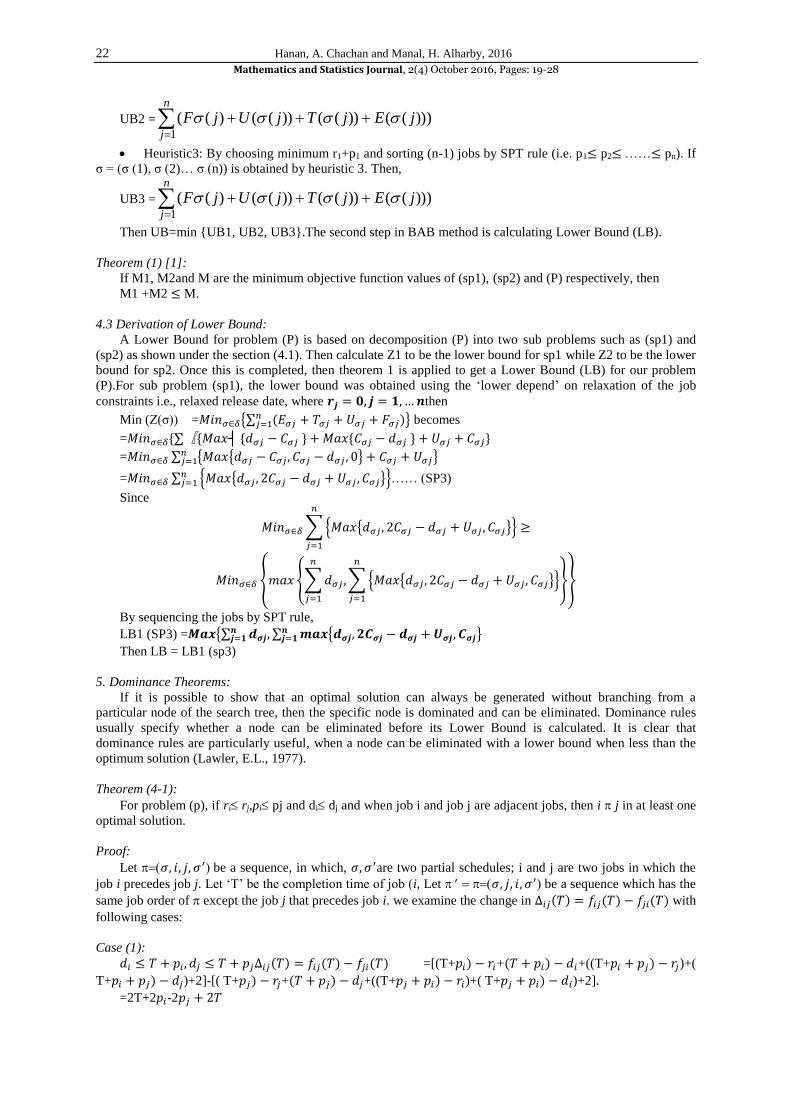
UB2 = )))(())(())(()((1

n

j

jEjTjUjF

Heuristic3: By choosing minimum r1+p1 and sorting (n-1) jobs by SPT rule (i.e. p1≤ p2≤ ……≤ pn). If

σ = (σ (1), σ (2)… σ (n)) is obtained by heuristic 3. Then,

UB3 = )))(())(())(()((1

n

j

jEjTjUjF

Then UB=min {UB1, UB2, UB3}.The second step in BAB method is calculating Lower Bound (LB).

Theorem (1) [1]:

If M1, M2and M are the minimum objective function values of (sp1), (sp2) and (P) respectively, then

M1 +M2 ≤ M.

4.3 Derivation of Lower Bound:

A Lower Bound for problem (P) is based on decomposition (P) into two sub problems such as (sp1) and

(sp2) as shown under the section (4.1). Then calculate Z1 to be the lower bound for sp1 while Z2 to be the lower

bound for sp2. Once this is completed, then theorem 1 is applied to get a Lower Bound (LB) for our problem

(P).For sub problem (sp1), the lower bound was obtained using the ‘lower depend’ on relaxation of the job

constraints i.e., relaxed release date, where 𝒓𝒋 = 𝟎, 𝒋 = 𝟏,…𝒏then

Min (Z(σ)) =𝑀𝑖𝑛𝜎∈𝛿{∑ (𝐸𝜎𝑗 + 𝑇𝜎𝑗 + 𝑈𝜎𝑗 + 𝐹𝜎𝑗)𝑛𝑗=1 } becomes

=𝑀𝑖𝑛𝜎∈𝛿{∑〖{𝑀𝑎𝑥┤ {𝑑𝜎𝑗 − 𝐶𝜎𝑗 } + 𝑀𝑎𝑥{𝐶𝜎𝑗 − 𝑑𝜎𝑗 } + 𝑈𝜎𝑗 + 𝐶𝜎𝑗}

=𝑀𝑖𝑛𝜎∈𝛿 ∑ {𝑀𝑎𝑥{𝑑𝜎𝑗 − 𝐶𝜎𝑗, 𝐶𝜎𝑗 − 𝑑𝜎𝑗 , 0} + 𝐶𝜎𝑗 + 𝑈𝜎𝑗}𝑛𝑗=1

=𝑀𝑖𝑛𝜎∈𝛿 ∑ {𝑀𝑎𝑥{𝑑𝜎𝑗 , 2𝐶𝜎𝑗 − 𝑑𝜎𝑗 + 𝑈𝜎𝑗 , 𝐶𝜎𝑗}}𝑛𝑗=1 …… (SP3)

Since

𝑀𝑖𝑛𝜎∈𝛿∑{𝑀𝑎𝑥{𝑑𝜎𝑗 , 2𝐶𝜎𝑗 − 𝑑𝜎𝑗 + 𝑈𝜎𝑗 , 𝐶𝜎𝑗}}

𝑛

𝑗=1

≥

𝑀𝑖𝑛𝜎∈𝛿 {𝑚𝑎𝑥 {∑𝑑𝜎𝑗 ,∑ {𝑀𝑎𝑥{𝑑𝜎𝑗 , 2𝐶𝜎𝑗 − 𝑑𝜎𝑗 + 𝑈𝜎𝑗 , 𝐶𝜎𝑗}}

𝑛

𝑗=1

𝑛

𝑗=1

}}

By sequencing the jobs by SPT rule,

LB1 (SP3) =𝑴𝒂𝒙{∑ 𝒅𝝈𝒋, ∑ 𝒎𝒂𝒙𝒏𝒋=𝟏

𝒏𝒋=𝟏 {𝒅𝝈𝒋, 𝟐𝑪𝝈𝒋 − 𝒅𝝈𝒋 +𝑼𝝈𝒋, 𝑪𝝈𝒋}

Then LB = LB1 (sp3)

5. Dominance Theorems:

If it is possible to show that an optimal solution can always be generated without branching from a

particular node of the search tree, then the specific node is dominated and can be eliminated. Dominance rules

usually specify whether a node can be eliminated before its Lower Bound is calculated. It is clear that

dominance rules are particularly useful, when a node can be eliminated with a lower bound when less than the

optimum solution (Lawler, E.L., 1977).

Theorem (4-1):

For problem (p), if rirj,pipj and didj and when job i and job j are adjacent jobs, then i j in at least one

optimal solution.

Proof:

Let 𝜎, 𝑖, 𝑗, 𝜎′be a sequence, in which, 𝜎, 𝜎′are two partial schedules; i and j are two jobs in which the

job i precedes job j. Let ‘T’ be the completion time of job (i, Let 𝜎, 𝑗, 𝑖, 𝜎′be a sequence which has the

same job order of except the job j that precedes job i. we examine the change in ∆𝑖𝑗(𝑇) = 𝑓𝑖𝑗(𝑇) − 𝑓𝑗𝑖(𝑇) with

following cases:

Case (1):

𝑑𝑖 ≤ 𝑇 + 𝑝𝑖 , 𝑑𝑗 ≤ 𝑇 + 𝑝𝑗∆𝑖𝑗(𝑇) = 𝑓𝑖𝑗(𝑇) − 𝑓𝑗𝑖(𝑇) =[(T+𝑝𝑖) − 𝑟𝑖+(𝑇 + 𝑝𝑖) − 𝑑𝑖+((T+𝑝𝑖 + 𝑝𝑗) − 𝑟𝑗)+(

T+𝑝𝑖 + 𝑝𝑗) − 𝑑𝑗)+2]-[( T+𝑝𝑗) − 𝑟𝑗+(𝑇 + 𝑝𝑗) − 𝑑𝑗+((T+𝑝𝑗 + 𝑝𝑖) − 𝑟𝑖)+( T+𝑝𝑗 + 𝑝𝑖) − 𝑑𝑖)+2].

=2T+2𝑝𝑖-2𝑝𝑗 + 2𝑇



Since (pi pj), then ∆𝑖𝑗(𝑇) ≤ 0 , 𝑖 → 𝑗

Case (2):

𝑑𝑖 ≤ 𝑇 + 𝑝𝑖 , 𝑇 + 𝑝𝑗 ≤ 𝑑𝑗 ≤ 𝑇 + 𝑝𝑖 + 𝑝𝑗

∆𝑖𝑗(𝑇) = 𝑓𝑖𝑗(𝑇) − 𝑓𝑗𝑖(𝑇) =[(T+𝑝𝑖) − 𝑟𝑖+(𝑇 + 𝑝𝑖 − 𝑑𝑖)+((T+𝑝𝑖 + 𝑝𝑗) − 𝑟𝑗)+(T+𝑝𝑖 + 𝑝𝑗) − 𝑑𝑗)+2]-[(

T+𝑝𝑗) − 𝑟𝑗+(𝑑𝑗 − (𝑇 + 𝑝𝑗))+((T+𝑝𝑗 + 𝑝𝑖) − 𝑟𝑖)+( T+𝑝𝑗 + 𝑝𝑖) − 𝑑𝑖)+1]

=(2(T+𝑝𝑖))-2𝑑𝑗

Hence ∆𝑖𝑗(𝑇) ≤ 0 , 𝑖 → 𝑗

Case (3):

𝑑𝑖 ≤ 𝑇 + 𝑝𝑖𝑇 + 𝑝𝑖 + 𝑝𝑗 , ≤ 𝑑𝑗

∆𝑖𝑗(𝑇) = 𝑓𝑖𝑗(𝑇) − 𝑓𝑗𝑖(𝑇)=[(T+𝑝𝑖) − 𝑟𝑖+(𝑇 + 𝑝𝑖 − 𝑑𝑖)+1+((T+𝑝𝑖 + 𝑝𝑗) − 𝑟𝑗)+(𝑑𝑗 −(T+𝑝𝑖 + 𝑝 𝑗 ))] - [(

T+𝑝𝑗) − 𝑟𝑗)+((𝑇 + 𝑝𝑗) − 𝑑𝑗) + 1+((T+𝑝𝑗 + 𝑝𝑖) − 𝑟𝑖)+(𝑑𝑖 − T+𝑝𝑗 + 𝑝𝑖))] =-2𝑝𝑗 ≤ 0

Hence 𝑖 → 𝑗

Case (4):

𝑇 + 𝑝𝑖 ≤ 𝑑𝑖 ≤ 𝑑𝑗 ≤ 𝑇 + 𝑝𝑖 + 𝑝𝑗 , ∆𝑖𝑗(𝑇) = 𝑓𝑖𝑗(𝑇) − 𝑓𝑗𝑖(𝑇) =-2T-2𝑝𝑗 + 2𝑑𝑖∆𝑖𝑗(𝑇)=2[T-𝑝𝑗 + 𝑑𝑖]≤ 0

Hence 𝑖 → 𝑗

Case (5):

𝑇 + 𝑝𝑖 ≤ 𝑑𝑖 , 𝑇 + 𝑝𝑗 ≤ 𝑑𝑗 ≤ 𝑇 + 𝑝𝑖 + 𝑝𝑗∆𝑖𝑗(𝑇) = 𝑓𝑖𝑗(𝑇) − 𝑓𝑗𝑖(𝑇)=[((T+𝑝𝑖) − 𝑟𝑖)+(𝑑𝑖 − (𝑇 +

𝑝𝑖))+((T+𝑝𝑖 + 𝑝𝑗) − 𝑟𝑗)+( T+𝑝𝑖 + 𝑝 𝑗 )−𝑑𝑗) + 1] - [( T+𝑝𝑗) − 𝑟𝑗)+(𝑑𝑗 − (𝑇 + 𝑝𝑗))+((T+𝑝𝑗 + 𝑝𝑖) − 𝑟𝑖)+(T+𝑝𝑗 +

𝑝𝑖)−𝑑𝑖 )+1].

2𝑑𝑖 − 2𝑑𝑗 Since di< dj

Hence 𝑖 → 𝑗

Case (6):

𝑇 + 𝑝𝑖 ≤ 𝑑𝑖 ≤ 𝑇 + 𝑝𝑖 + 𝑝𝑗 ≤ 𝑑𝑗∆𝑖𝑗(𝑇) = 𝑓𝑖𝑗(𝑇) − 𝑓𝑗𝑖(𝑇) =[((T+𝑝𝑖) − 𝑟𝑖)+(𝑑𝑖 − (𝑇 + 𝑝𝑖))+((T+𝑝𝑖 +

𝑝𝑗) − 𝑟𝑗)+( 𝑑𝑗-(T+𝑝𝑖 + 𝑝 𝑗 )] - [( T+𝑝𝑗) − 𝑟𝑗)+(𝑑𝑗 − (𝑇 + 𝑝𝑗))+((T+𝑝𝑗 + 𝑝𝑖) − 𝑟𝑖)+(𝑑𝑖 -(T+𝑝𝑗 + 𝑝𝑖) )].

=2[(𝑑𝑖 − (𝑇 + 𝑝𝑖 + 𝑝𝑗)]

Since 𝑑𝑖 ≤ 𝑇 + 𝑝𝑖 + 𝑝𝑗

Then Hence 𝑖 → 𝑗

Case (7):

𝑇 + 𝑝𝑖 + 𝑝𝑗 ≤ 𝑑𝑖 ≤ 𝑑𝑗∆𝑖𝑗(𝑇) = 𝑓𝑖𝑗(𝑇) − 𝑓𝑗𝑖(𝑇) =[((T+𝑝𝑖) − 𝑟𝑖)+(𝑑𝑖 − (𝑇 + 𝑝𝑖))+((T+𝑝𝑖 + 𝑝𝑗) − 𝑟𝑗)+( 𝑑𝑗-

(T+𝑝𝑖 + 𝑝 𝑗 )] - [( T+𝑝𝑗) − 𝑟𝑗)+(𝑑𝑗 − (𝑇 + 𝑝𝑗))+((T+𝑝𝑗 + 𝑝𝑖) − 𝑟𝑖)+(𝑑𝑖 -(T+𝑝𝑗 + 𝑝𝑖) )].=𝑑𝑖 + 𝑑𝑗 − 𝑑𝑗 − 𝑑𝑖 = 0

Then Hence 𝒊 → 𝒋

6. Local Search Heuristic Method:

In this section, we reviewed the local search techniques that are useful in solving single machine scheduling

problems. ‘Local search’ is an iterative algorithm that moves from one solution ‘𝑠’to another ‘𝑠′’according to

some neighborhood structure. The Local search algorithm provides a robust approach to obtain high quality

solutions to problems of a realistic size in reasonable time. The Local search procedure usually consists of the

following steps.

1. Initialization: Choose an initial schedule 𝑠to be the current solution and compute the value of the objective

function𝐹(𝑠). 2. Neighbor Generation: Select a neighbor 𝑠′ of the current solution 𝑠 and compute 𝐹(𝑠′). 3. Acceptance Test: Test whether accept the move from 𝑠to𝑠′. If the move is accepted, then 𝑠′ replaces 𝑠 as the

current solution; otherwise 𝑠is retained as the current solution.

4. Termination Test: Test whether the algorithm should be terminated. If it is terminated, then generate the

best output solution or otherwise, return to the neighbor generation step.

We assume that a schedule is represented as a permutation of job numbers(𝑗1, 𝑗2, … , 𝑗𝑛). This can always be

done for a single machine processing system or for permutation flow shop; for other models, more complicated

structures are used. In the first step, a starting solution can be specified by a random job permutation. If local



search procedure is applied several times, then it is reasonable to use random initial schedules. To generate a

neighbor 𝑠′in Step (2), a neighborhood structure should be specified beforehand. The following types of

neighborhoods are considered often.

Transpose neighborhood in which the two jobs that occupy the adjacent positions in the sequence are

interchanged:

(1, 2, 3, 4, 5, 6, 7) (1, 3, 2, 4, 5, 6, 7);

swap neighborhood in which two arbitrary jobs are interchanged.

(1, 2, 3, 4, 5, 6, 7) (1, 6, 3, 4, 5, 2, 7);

Neighbors can be generated randomly, systematically, or through some combination of the two approaches.

In Step (3), the acceptance rule is usually based on the values and of the objective function

for schedules & . In some algorithms, the moves to ‘better’ schedules are only accepted (schedule is

better than if ); while in others, it may be allowed to move to ‘worse’ schedules also.

Sometimes ‘wait and see’ approach is adopted.

The algorithm terminates in Step (4) if the computation time exceeds the pre-specified limit or after

completing the pre-specified number of iterations.

6.1Simulated Annealing(SA) (Ingber, L., 1993):

Simulated Annealing is an algorithmic method which is able to escape from local minima. It is a

randomized local search method for two reasons:

First, from the neighborhood of a solution, a neighbor which is always accepted when selected, the worse-

cost neighbors are also accepted though it is gradually decreased with a probability in the course of action. The

randomized nature enables asymptotic convergence to optimum solutions under certainand mild conditions.

Nevertheless, the energy landscape, which is determined by the objective function and the neighborhood

structure may admit many and/or ‘'deep 'local minima. Therefore, avoiding local minima is a crucial part in the

performance of an algorithm.

Algorithm for Simulated Annealing (SA):

Step (1):

Select an initial solution s∈ 𝑆,s* and select an initial temperature tO> 0 ;k=0,G=1:

Step (2):

Define B; Choose s'∈ 𝑁∗(𝑠); ∆= 𝑓(𝑠′) − 𝑓(𝑠) P (∆, 𝑡𝑘)=exp(-∆/𝑡𝑘);

If∆≤ 0 then s=s', and if f(s)< 𝑓(𝑠∗), then s*=s, else (∆> 0);

if a random number of[0,1]≤ 𝑃(∆, 𝑡𝑘),then s=s';G=G+1

Step (3):

if G≤ 𝐵 return to step (2).

Step (4):

Update temperature; k=k+1; return to step(2)until some stopping criteria are met.

6.2Threshold Acceptance Method (TH)( DUECK, G. and T. SCHEUER, 1990):

A variant of Simulated Annealing is the Threshold Acceptance Method Brucker (2007). It differs from

Simulated Annealing only by the acceptance rule for the randomly generated solution𝑠′ ∈ 𝑁. 𝑠′is accepted if the

difference 𝐹(𝑠′) − 𝐹(𝑠) is smaller than some non-negative threshold t. The positive control parameter‘t’is

gradually reduced.The Threshold Acceptance Method has the advantage that they can leave a local minimum.

But there is a disadvantage that it is possible to get back to solutions that were already visited. Therefore

oscillation around local minima is possible and this may lead to a situation where much computational time is

spent on a small part of the solution set.

6.3 Descent Method (DM)( FERLAND, J.A., et al., 1996):

In a simple local search algorithm, such as a Descent Algorithm, an initial solution is chosen at random and

then a neighboring solution is generated based on some mechanism. If the neighboring solution is better than the

current solution, it replaces the current solution or otherwise the current solution is retained. The process is

repeated until no improving neighbor is found for the current solution.

6.4 Algorithm: Improvement Descent algorithm (DM):

Step (1):

Choose initial solution s∈S.



Step (2):

Generate (s/) neighborhood for (s) (by insert or swap) and set∆= 𝑓(𝑠′) − 𝑓(𝑠), if ∆< 0 then set s=s'.

Step (3):

If𝑓(𝑠′) ≥ 𝑓(𝑠)∀𝑠 ′ ∈ 𝑁(𝑆), then stop; else return to step (2).

The local search methods (TH), (SA) and (DES) stopped when iteration =1000 iterations.

7. Computational experience:

An intensive work of numerical experimentations has been performed. Firstly, we presented how instances

(tests problem) can be randomly generated. There exists in the literature, a classical way to randomly generate

tests problem of scheduling problems.

The processing time Pi is uniformly distributed in the interval (Abbas, I.T., 2009; Fry, T.D., et al.,

1996).

The release date ri is uniformly distributed in the interval (Abbas, I.T., 2009; Fry, T.D., et al., 1996).

The due dates di are uniformly distributed in the interval [P (1−TF−RDD/2), P (1+TF+RDD/2)]; where

P=∑Pi , depending on the relative Range of Due Date (RDD) and on the average Tardiness Factor (TF). For

both parameters, values such as 0.2, 0.4, 0.6, 0.8 and 1.0 are considered. For each selected value of ‘n’, two

problems were generated for each values of parameters producing 10 problems for each values of n.

The BAB algorithm was tested in Fortran Power Station and local search methods (Threshold Acceptance

Method (TH), Descent Methods (DM) and Simulated Annealing (SA)). This was tested first in coding followed

by MATLAB R2009b running on Personal Computer with configuration (Pentium (R) at 2.20 GHz with Ram 2

GB computer processor-type PDCT 4400).

In table (1), the value of n is listed as 7 jobs and 11 jobs. We listed five problems for each value of n. Test

problems are tested to show the efficiency of our Lower Bound (LB) used in BAB algorithm to obtain the

optimal solution. The results comparing the Lower Bound, Upper Bounds and the optimal solutions are given in

table (1). The three columns are the number of problems, the number of examples and the value of an optimal

solution found by BAB algorithm respectively. The fourth column gives the value of the Initial Lower Bound

(ILB). The fifth, sixth and the seventh columns give the value of our Upper Bounds (UB1, UB2 and UB3). The

eight columns gives the number of nodes (Nodes).

Table 1: The performance of initial lower bound, upper bounds number of nodes of BAB algorithm

N Number Opt. ILB UB1 UB2 UB3 Nodes

7 1 259 235 311 286 304 25

2 205 143 254 249 220 48

3 127 61 191 143 130 68

4 173 122 231 187 209 25

5 206 188 224 211 283 43

11

1 372 287 412 389 479 164

2 376 274 611 453 459 136

3 297 189 425 328 332 494

4 410 314 608 440 488 127

5 384 337 499 442 459 136

Opt. = the optimal value obtained by BAB algorithm.

ILB = Initial lower bound.

UB1, UB2 and UB3 = Upper bounds.

Nodes = the number of generated nodes.

Table (1) shows the lower and upper bounds, the number of nodes and computational time for five

problems of n=7, n=10 jobs. It was observed that whenever there is an increase in number of nodes and

computational time when ‘n’ increases.

7.1 Comparative Results for Local Search Methods:

The Table (2) shows the comparison between local search methods which are TH, SA and Des. The results

in table (2) show that (SA) has good performance results, followed by (TH) and (Des).



Table 3: comparison between Local Search Methods

N = 50

N TH SA DES Best

1 10262 7709 11260 7709

2 8268 7765 11404 7765

3 9236 7591 11359 7591

4 9753 7609 11239 7609

5 10389 7749 11107 7749

6 10755 7659 11459 7659

7 10614 7640 11454 7640

8 10298 7527 11383 7527

9 11303 7793 11445 7793

10 11390 7711 11422 7711

No. of best - 10 -

Av. time 0.0218 0.1279 0.1391 -

N = 200

1 174363 113191 173047 113191

2 174150 113195 150980 113195

3 173952 113091 168930 113091

4 174361 113025 177719 113025

5 174369 113198 177818 113198

6 174321 113074 174581 113074

7 174066 112990 167732 112990

8 174375 113204 178612 113204

9 173806 113181 190749 113181

10 174373 113085 203557 113085

No. of best - 10 - -

Av. time 1.265881 0.01451 0.030966 -

N = 600

1 1077347 683850 1076326 683850

2 1077485 684105 1058664 684105

3 1077300 684037 1041905 684037

4 1076996 683912 1124454 683912

5 1077418 684001 1029818 684001

6 1077428 684011 1058602 684011

7 1077382 684154 1101603 684154

8 1077440 684108 1104567 684108

9 1077437 684109 1101084 684109

10 1077402 684046 1271732 684046


Av. time 0.4508 0.4238 0.2003 -

N=700

1 1505420 954150 1502573 954150

2 1503871 954203 1523971 954203

3 1503747 955378 1561154 955378

4 1502101 954626 1561661 954626

5 1505531 954924 1503419 954924

6 1505328 954924 1539732 954924

7 1503825 954214 1581539 954214

8 1503662 955317 1575105 955317

9 1503671 955412 1655246 955412

No. of best - 10 -

Av. time 0.5194 0.5963 0.1823

N=1000

1 4458371 2805479 4457383 2805479

2 4458637 2805619 4132681 2805619

3 4458507 2805458 4240319 2805458

4 4458318 2805597 4529852 2805597

5 4458633 2805631 4115818 2805631

6 4458605 2805643 4135173 2805643

7 4458524 2805523 4482102 2805523

8 4458358 2805586 4383169 2805586

9 4458603 2805621 4639244 2805621

10 4458540 2805628 4961876 2805628


Av. time 0.9041 0.9890 0.2336 -

SA= Simulated Annealing

TH =Threshold Acceptance Method



DM=Descent Methods

Best = Best solution by using MA, TH and TS

No. of best = Number of best solutions

Av. time = Average time of ten examples

Conclusion:

This study investigated the problem of scheduling jobs in one machine to minimize bi-criteria with release

date. The four criteria to be minimized are ∑Fi,∑Ui,, ∑Ti and ∑Ei. The current study deployed ‘Branch and

Bound’ algorithm to find the optimal solution for the problem of minimizing a linear function (i.e., ∑ (Fi+ Ui,+

Ti +Ei). A computational experiment that consists on a large set of test problems are given for BAB algorithm

which solve the test problem up to (29) jobs. The NP−hardness of this problem and the optimal solutions of the

BAB algorithm are not quick in their responses. Hence, this problem is solved by local search methods such as

Descent Methods, Threshold Acceptance Method and Simulated Annealing. Further the results of extensive

computations test of local search methods were also compared in this study. The main conclusion to be drawn

for our computation results is that SA is more effective method for the chosen problem, followed by TH and

DM.

9. Future Work:

An interesting future research topic would involve experimentation with the following problems such as F2/

ri / ∑Ci + Lmax and 1/ri / ∑Ci + Lmax + Emax .

REFERENCES

Abbas, I.T., 2009. "The performance of

multicriteria scheduling in one machine", M.Sc.

Thesis Univ.of Al-Mustansiriyah, Collage of

Science, Dept. of Mathematics.

B¨ulb¨ul, K., P. Kaminsky, C. Yano, 2007.

Preemption in single machine earliness/tardiness

scheduling. Journal of Scheduling, 10: 271-292.

Brucker, P., 2007. "Scheduling Algorithms",

Springer BerlinHeidelberg New York, Fifth Edition.

Chang, P.C., 1999. A branch and bound

approach for single machine scheduling with

earliness and tardiness penalties. Computers and

Mathematics with Applications, 37: 133-144.

Cyril Briand1, a, b, 2011. Samia Ouraric''

Minimizing the number of tardy jobs for the single

machine scheduling problem: MIP-based lower and

upper bounds '' Preprint submitted to RAIRO-OR.

Davis, J.S., J.J. Kanet, 1993. Single-machine

scheduling with early and tardy completion costs.

Naval Research Logistics, 40: 85-101.

Detienne, B., E. Pinson, D. Rivreau, 2010.

Lagrangian domain reductions for the single

machine´ earliness-tardiness problem with release

dates, European Journal of Operational Research,

201: 45-54.

DUECK, G. and T. SCHEUER, 1990.

“Threshold accepting: a general purpose optimization

algorithm appearing superior to simulated

annealing”, Journal of Computational Physics, 90:

161-175.

FERLAND, J.A., A. HERTZ and A. LAVOIE,

1996. “An object oriented methodology for solving

assignment type problems with neighborhood search

techniques”, Operations Research, 44: 347-359.

Fry, T.D., R.D. Armstrong, K. Darby-Dowman,

P.R. Philipoom, 1996. A branch and bound

procedure to minimize mean absolute lateness on a

single processor. Computers & Operations Research,

23: 171-182.

Hoogeveen, J.A., S.L. van de Velde, 1996. A

branch-and-bound algorithm for single-machine

earliness-tardiness scheduling with idle time.

INFORMS Journal on Computing, 8: 402-412.

Kim, Y.-D., C.A. Yano, 1994. Minimizing mean

tardiness and earliness in single-machine scheduling

problems with unequal due dates. Naval Research

Logistics, 41: 913-933.

Kellerer, H., T. Tautenhohn and G.J. Woeginger,

1996. "Approximability and non-approximability

results for minimizing total flow time on a single

machine." Proceedings of the 28th Annual ACM

symposium on theory of Computing, 418-426 SIAM

Journal on Computing

Ingber, L., 1993. "Simulated annealing: practice

versus theory", Math. Comput. Modelling 18, 11, 29-

57. 2. Deboeck, G. J. [Ed.], "Trading On the Edge",

Wiley, 1994.

Lawler, E.L., 1977. A “pseudo polynomial”

algorithm for sequencing jobs to minimize total

tardiness, Annals of Discrete Mathematics, 1: 331-

342.

Lenstra, J.K., A.H.G Rinnooy Kan and P. Brucker, "Complexity of machine scheduling

problems, Annals of Discrete Mathematics, 1: 343-

362.

Mason, A.J. and E.J. Anderson, 1991.

"minimizing flow time on a single machine with job

classes and setup times" Naval Research Logistics,

38: 333-350.

Michael, J. Moore, 1968. “An n job, one

machine sequencing algorithm for minimizing the

number of late jobs”, Management Science, 15(1):

102-109.



Pinedo, M., 1995."Scheduling: theory,

algorithms, and systems. Englewood Cliff, NJ:

Prentice Hall

Sourd, F., S. Kedad-Sidhoum, 2003. The one-

machine problem with earliness and tardiness

penalties. Journal of Scheduling, 6: 533-549.

Sourd, F., S. Kedad-Sidhoum, 2008. : A faster

branch-and-bound algorithm for the earliness-

tardiness scheduling problem. Journal of Scheduling,

11: 49-58.

Sourd, F., 2009. New exact algorithms for one-

machine earliness-tardiness scheduling. INFORMS

Journal on Computing, 21: 167-175.

Yano, C.A., Y.-D. Kim, 1991. Algorithms for a

class of single-machine weighted tardiness and

earliness problems. European Journal of Operational

Research, 52: 167-178.

Yau, H., Y. Pan, L. Shi, 2008. New solution

approaches to the general single machine earliness

tardiness problem. IEEE Transactions on Automation

Science and Engineering, 5: 349-360.

Zghair, M.K., 2000. "Single machine scheduling

to minimize total cost of flow time with unequal

ready times", Journal of Basrah Researches, 25(3):

94-108.

issn-2077-4591 mathematics and statistics journal...

Documents