issues in structural health monitoring employing smart sensors
TRANSCRIPT

Issues in Structural Health Monitoring Employing Smart Sensors
T. Nagayama1, S. H. Sim1, Y. Miyamori2, and B. F. Spencer, Jr.3
ABSTRACT
Smart sensors densely distributed over structures can provide rich information for
structural monitoring using their onboard wireless communication and computational
capabilities. However, issues such as time synchronization error, data loss, and dealing
with large amounts of harvested data have limited the implementation of full-fledged
systems. Limited network resources (e.g., battery power, storage space, bandwidth, etc.)
make these issues quite challenging. This paper first investigates the effects of time
synchronization error and data loss, aiming to clarify requirements on synchronization
accuracy and communication reliability in SHM applications. Coordinated computing is
then examined as a way to manage large amounts of data.
Keywords: coordinated computing; data compression; distributed computing strategy;
smart sensors; time synchronization; data loss; data aggregation
1. INTRODUCTION
The investment of the United States in civil infrastructure is estimated to be $20 trillion.
Annual costs amount to between 8-15% of the GDP for most industrialized countries
1 Doctoral Candidate, Dept. of Civil and Environmental Engineering, University of Illinois at Urbana-Champaign, Urbana, IL 61801, USA 2 Assistant Professor, Kitami Institute of Technology, Hokkaido 090-8507, Japan 3 Nathan M. and Anne M. Newmark Endowed Chair of Civil Engineering, University of Illinois at Urbana-Champaign, Urbana, IL 61801, USA

(U.S. Census 2004; Jensen 2003). This investment is likely to increase; for example, the
U.S. Department of Transportation (2003) has reported that the capital investment to
preserve highways and bridges increased 45.7% from $23.2 billion in 1997 to $33.6
billion in 2000. Indeed, much attention has been focused in recent years on the declining
state of the aging infrastructure in the U.S. These concerns apply not only to civil
engineering structures, such as the nation's bridges, highways, and buildings, but also to
other types of structures, such as the aging fleet of aircraft currently in use by domestic
and foreign airlines. The ability to continuously monitor the integrity of civil
infrastructures in real-time offers the opportunity to reduce maintenance and inspection
costs, while providing for increased safety to the public. Furthermore, after natural
disasters, it is imperative that emergency facilities and evacuation routes, including
bridges and highways, be assessed for safety. Addressing all of these issues is the
objective of structural health monitoring (SHM).
To efficaciously investigate damage, a dense array of sensors is required for
large civil engineering structures. (Spencer et al. 2004, Gao 2005). Dense measurement
is expected to provide detailed information on civil infrastructure, which typically
consists of a large number of components and has many degrees of freedom. Monitoring
the Tsing Ma Bridge and Kap Shui Mun Bridge in Hong Kong, which uses 326 channels
of sensors and produces about 65 MB of data every hour, is an attempt toward in-depth
monitoring (Wong 2004). Expensive installation of traditional monitoring systems,
however, has limited significantly wider spread implementation (Lynch and Loh 2006,
Farrar 2001, and Celebi 2002). Smart sensors with wireless communication capability
are reported to reduce installation effort to a great extent (Lynch et al. 2005) and help to
realize a dense array of sensors.

Though networks of densely deployed smart sensors have the potential to
improve SHM dramatically, limited resources on smart sensors preclude direct
application of traditional monitoring strategies on smart sensor networks. Time
synchronization among smart sensors is not as accurate as for a wired system. Data
transfer between sensor nodes is less reliable than in a wired system due to data loss.
Transferring all data to a central station using wireless communication is not practical or
scalable, especially in a system employing a dense array of smart sensors. Moreover,
battery power often imposes practical limits on these functionalities. Although many
researchers have reported difficulties in data transfer rates and reliability, as well as time
synchronization (Casciati et al. 2003, Elson et al. 2002, Kottapalli et al. 2003, Mechitov
et al 2003, Mosalam 2003, Kurata et al. 2004 Wang et al. 2005), the effects on SHM and
ways to address these issues have not been studied in depth. Careful investigation can
provide insight into how to accommodate these difficulties from a SHM perspective.
This paper studies issues associated with SHM applications employing smart
sensor networks. Several issues critical to realizing a SHM system using smart sensors
are first described. Among them, the effects of time synchronization error and data loss
are investigated from a SHM perspective. Coordinated computing is examined as a way
to manage large amounts of data. Numerical simulation and experimental testing
validate the derivation and proposals.

2. SHM EMPLOYING SMART SENSORS
Smart sensors with computational and communication capabilities have been employed
for SHM research. Some of the first efforts in developing smart sensors for application
to civil engineering structures were presented by Straser and Kiremidjian (1996, 1998)
and Kiremidjian et al. (1997). Since these initial efforts, numerous researchers have
developed smart sensing platforms (Lynch and Loh 2005). With respect to functionality,
most of early attempts simply replaced wired communication with RF links. Together
with introduction of battery power at the sensor nodes, RF communication eliminated
the need for cabling. Such measurement systems with wireless communication links,
however, encounter many difficulties, e.g., slow and unreliable communication,
inaccurate time synchronization among sensor nodes, insufficient sensing capabilities,
and limited power. While smart sensor’s computational capability potentially offers new
opportunities for SHM, these issues need to be carefully examined before a functional
SHM system can be realized.
Among the issues is lossy RF communication, which can severely impair a
SHM system. Structural analysis generally assumes data acquired at specified time
interval is available with certain accuracy. While measurement noise and quantization
errors are usually considered primary sources of errors, data loss has not been
considered as an error source in traditional SHM systems because all the data is reliably
transferred in a wired system. This assumption does not apply to wireless systems;
many researchers have reported data loss during wireless communication (Casciati et al.
2003, Mosalam 2003, Kurata et al. 2004). Mechitov et al. (2003) addressed this
communication reliability problem by utilizing acknowledgement messages. However,
4

reliable communication is stated to be slow due to associated header information and
acknowledgement messages, using more resources of a system. Studies of the data loss
effect on structural analysis are needed to assess the use of more expensive reliable
communication versus simple lossy communication.
Time synchronization error in a smart sensor network is another source of
inaccuracy in SHM applications. Each sensor node has its own clock. By
communicating with surrounding nodes, smart sensors can assess relative difference
among their local clocks. Well-known algorithms include Reference Broadcast
Synchronization (Elson et al. 2002), Flooding Time Synchronization Protocol (Maroti et
al. 2004), and Timing-sync Protocol for Sensor Networks (Ganeriwal et al. 2003). Time
synchronization is, however, not as accurate as for a wired networked system. Also, the
local clock of a smart sensor can have large drift in time and need to synchronize with
each other repeatedly to maintain certain synchronization accuracy. Time
synchronization error problems have been reported both in laboratory and in full-scale
bridge monitoring applications using smart sensors (Lynch et al. 2005). Requirements
on synchronization accuracy need to be investigated from a SHM perspective.
Data aggregation is especially problematic for SHM applications which
typically require large amounts of data. For example, 2-byte data samples collected at
100 Hz generate 12 KB of data every minute. While the CC1000, one of RF chips
adapted in several early smart sensor platforms, supports 38.4kbps data rate, the actual
rate at which measurement data is transferred is much slower because of packet
collision, packet headers, etc. Acknowledgement messages associated with reliable
communication reduce data transfer speeds even more. A centralized data collection
5

system, which simply replaces the wired links of a traditional SHM system with RF
links, therefore, cannot handle the massive amounts of data acquired concurrently at
hundreds of sensor nodes (see Fig. 1).
Several researchers have attempted to address the data aggregation problem.
Tiered networks (Govindan et al. 2005) help centrally collect a large amount of data
using several powerful master nodes together with smart sensor end nodes, though the
usage is limited to applications in which use of powerful master nodes is viable; cost to
install master nodes and the number of required master nodes are factors in determining
its practicality. Another approach to address this data aggregation problem is
independent data processing as shown in Fig. 2. Each smart sensor independently
measures and processes data, typically using same pattern recognition, without sharing
information among the neighboring nodes (Sohn et al. 2002, Lynch et al. 2005, Nitta et
al. 2005). Because only the processed data is sent back to the base station,
communication requirements are relatively small. However, from a SHM perspective,
this approach can not utilize available spatial information from neighboring nodes (e.g.
mode shapes). The inability of this approach to incorporate spatial information limits its
effectiveness in SHM applications. Data aggregation utilizing distributed computing
(Gao 2005, Nagayama et al. 2006) has the potential to achieve effective SHM
employing smart sensors. Application specific knowledge is utilized to efficiently
aggregate information in a distributed and coordinated manner (see Figure 3). Though
this concept has been proposed, only partial implementation of this concept has been
reported so far (Nagayama et al 2006). Implementation of the concept is expected to
demonstrate a way to address the data aggregation problem in SHM applications.
6

Data acquisition
Data processing
Data acquisition
Data processing
Fig. 1 Centralized data collection
Data acquisition & processingData acquisition & processing
Fig. 2 Independent data processing
Data acquisition
Outcome forwarding
Data processingIn communities
Data acquisition
Outcome forwarding
Data processingIn communities
Fig. 3 Coordinated computing strategy
3. EFFECT OF TIME SYNCHRONIZATION ERROR ON SHM
Time synchronization error in a smart sensor network can cause inaccuracy in SHM
applications. Time synchronization is a middleware service common to smart sensor
applications and has been widely investigated. Each smart sensor has its own local clock,
which is not synchronized initially with other sensor nodes. By communicating with
surrounding nodes, smart sensors can assess relative difference among their local clocks.
For example, Mica2 motes employing TPSN are reported to synchronize with each
other to an accuracy of 50μsec; different algorithms and hardware resources may result
in different precision. Whereas time synchronization protocols have been intensively
studied, requirements on synchronization from an application perspective are lacking. In
many SHM applications, commonly used quantities include cross spectral density
7

(CSD), power spectral density (PSD), correlation function, and modal parameters. The
effects of synchronization error on these estimates are discussed in this section.
3.1. Modeling of time synchronization error
Consider a signal from a smart sensor in local clock coordinate ( )x t can be written
using a signal in the reference clock, or the global clock ( )x t as
( )( )( ) 1 jx t x t tα= + − Eq. (1)
where tj is the initial time synchronization error and α is the clock drift rate. In the
frequency domain, this relationship is expressed as
11( )1 1
jti
X e Xω
α ωωα α
−+ ⎛= ⎜+ +⎝ ⎠
⎞⎟ Eq. (2)
where ( )X ω and ( )X ω are the Fourier transform of ( )x t and ( )x t , respectively.
Clock drift is oftentimes small. In the following derivation α is assumed to be zero.
3.2. Impact of time synchronization error in input-output identification
Change in the estimation of modal parameters due to the poorly synchronized input and
output can be identified by looking into the transfer function. If the m-th input and n-th
output are shifted by and , respectively, the transfer function inmt
outnt ( )nmH ω between
the shifted input and output is written as
( )( ) ( )( ) ( )
( ) ( )
( )
outn in out
m ninm
nm
i ti t tn n
nm nmi tm mi t
nm
Y e YH eF e F
e H
ωω
ω
ω
ω ω Hω ωω ω
ω
−−
−= = =
=
Eq. (3)
where = – . From nmt inmt
outnt Eq. (3), the magnitude of transfer function remains
8

unchanged while its phase is shifted by . When modal parameters are estimated
from this transfer function, the natural frequency, damping ratio, and magnitude of the
mode shape remain unchanged; only the phase of mode shapes is affected by the time
synchronization error. The phase shift
nmt
kφ of the k-th mode is estimated as follows,
2k k nmf tφ π= Eq. (4)
where kf is the natural frequency of the k-th mode.
3.3. Impact of time synchronization error in output-only identification
The effect of time synchronization errors on modal parameters such as the natural
frequency, damping ratio, and mode shape are examined for the case when only output
measurement is available. When the excitation can be assumed to be broadband and the
structural response stationary, the correlation function between the output measurements
can be used to determine modal parameters by virtue of the Natural Excitation
Technique (NExT) (James et al. 1992). Investigating the correlation function, change in
modal parameters due to the time synchronization inaccuracy can be identified.
For completeness, NExT is briefly reviewed here. Consider the equation of
motion in Eq. (5) under the assumption that the random responses are stationary.
( ) ( ) ( )( )Mx t Kx t f tCx t+ + = Eq. (5)
where M , , and are the n x n mass, damping, and stiffness matrices,
respectively;
C
(
K
)x t is a n x 1 displacement vector; ( )f t is a m x 1 force vector; ( )x t
and ( )x t are the velocity and the acceleration vector. By multiplying displacement at
reference sensor and taking expected value, Eq. (5) is transformed as follows.
9

Eq. (6) ( ) ( ) ( ) ( )
( ) ( ) ( ) ( )
ref ref
ref ref
ME x t x t CE x t x t
KE x t x t E f t x t
τ τ
τ τ
⎡ ⎤ ⎡ ⎤+ + +⎣ ⎦ ⎣⎡ ⎤ ⎡+ + = +⎣ ⎦ ⎣
⎦⎤⎦
Because the input force and response at the reference sensor location are uncorrelated
for 0τ ≥ , the right hand side is zero. The expectation between the two signals is the
correlation function. Therefore, by denoting [ ]( ) ( )E x t y tτ+ as the correlation function
( )xyR τ , Eq. (6) is rewritten as
( ) ( ) ( ) 0, 0.ref ref refxx xx xxMR CR KRτ τ τ τ+ + = > Eq. (7)
When and ( )A t ( )B t are weakly stationary processes, the following relation holds
(Bendat and Piersol 2000).
( ) ( )ABABR Rτ τ= Eq. (8)
A similar relation holds for higher derivatives.
( )( )( ) ( )mm
ABA BR Rτ τ= Eq. (9)
where the superscript, m, denotes the m-th derivative. Consequently, Eq. (7) can be
rewritten as
( ) ( ) ( ) 0, 0.ref ref refxx xx xxMR CR KRτ τ τ τ + + = > Eq. (10)
Thus, the correlation function for the stationary responses is shown to satisfy the
equation of motion for free vibration. This fact can be directly used for modal analysis
such as Eigensystem Realization Algorithm (ERA) (Juang and Pappa 1985).
Time synchronization errors enter into correlation function estimation.
Consider a cross correlation function ( )i refx xR τ between a response ( )ix t at location i
10

and the reference signal ( )refx t . The sensor node at location i has a time
synchronization error of ixt relative to the reference node. The correlation function,
( )i refx xR τ , under the synchronization error, can be written as
( ) ( ) ( ) ( )i i ref ii refx x i x ref x x xR t E x t t x t R t tτ⎡ ⎤= − + = −⎣ ⎦ Eq. (11)
If ixt is positive, the correlation function for the interval (0,
ixt ) does not have the
same characteristics as the succeeding signal. In a structural analysis context, this
portion has negative damping; therefore, the beginning portion of the signal needs to be
removed. When ixt is unknown, a segment corresponding to the maximum possible
time synchronization error, , is truncated from the correlation function. maxxt
( )( )
( )( )
1
1
1 1
n
m x
R A
ϕ
φ λ
φ λ
φ λ
λτ
Λ
The correlation functions, each having independent time synchronization errors,
do not satisfy the equation of motion, Eq. (10). The correlation functions after the
truncation, however, can be decomposed into modal components as follows
( ) ( )( ) (
( ) (( ) ( )
1 1
2 2
' '
'2
11 21 2 2 1 2
12 22 2 2 2 2
2 2 2 2
1 2 2
( )
'
ex exp exp
exp exp exp
ex exp exp
exp exp
ref
m m
x x
x x n
x x n
m x nm n
n
t t
t t
t t
diag
τ
ϕ ϕ
φ λ φ λ
φ λ φ λ
φ λ φ λ
λ τ λ τ
= Φ
⎡ ⎤Φ = ⎣ ⎦' '1 2
'
p
p
exp
)
)
1
2
m
n x
n x
x
t
t
t
⎡ ⎤− − −⎢ ⎥⎢ ⎥− − −⎢ ⎥=⎢ ⎥⎢ ⎥
− − −⎢ ⎥⎣ ⎦
Λ = ⎡⎣( )
Eq. (12)
[ ]( )
2
1 2 2
1i i i i
n
h
A diag a a
λ ω ω
⎤⎦
= − + −
=ih j
a
where ' ' ( )refx xR τ is the correlation function matrix on the interval ( )max
,xt ∞ , ijφ is j-th
11

element of i-th mode shape, hi and ωi are i-th modal damping ratio and modal natural
frequency, respectively, and ai is a factor accounting for the relative contribution of the
i-th mode in the correlation function matrix. Modal analysis techniques such as ERA
can be used to identify these modal parameters. As Eq. (12) shows, the natural
frequencies and damping ratios remain the same. The observed mode shapes ' are
different from the original mode shapes; changes in mode shape amplitude are
negligible due to small hi and
Φ
ixt , while phase shift can be meaningful. Mode shape
phases can indicate structural damage and are important modal characteristics from a
SHM perspective (Nagayama et al. 2005). Time synchronization error of 1ms results in
about 3.6 degree phase delay of a mode at 10 Hz, while the same time synchronization
error causes 36 degree phase delay at 100 Hz. The phase delay tolerance depends on the
applications. When change in phase is investigated as in Nagayama et al. (2005), even
3.6 degree phase delay is considered to obscure the detail. The requirements on the time
synchronization for modal analysis need to be assessed mainly from the viewpoint of
mode shape phases.
3.4. Numerical simulation in 2 DOF model
To confirm the analytical investigation in the previous section, a numerical simulation is
conducted using the 2 DOF model shown in Fig. 4. In this example, the natural
frequencies and damping ratios of the model are listed in Table 2. Two independent
band limited white noise inputs are imposed on the nodes, and accelerations of the
lumped masses are simulated with the sampling time of 1 msec. 50 sample time
histories are obtained for different input excitations and each time history is 81.91
seconds long. Several cases of time synchronization errors ( τΔ =1, 3, 5, 10, 25, 50, 100
12

msec) are considered for the simulated acceleration data of the 2nd nodal point.
B.L.W.N
y1
y2
k1
k2
m1
m2
Fig. 4 Analytical model
Table 1 2DOF model
Mass (kg) m1 1 m2 2
Stiffness (N/m) k1 200 k2 400
Table 2 Natural frequency and damping ratio
Mode Natural frequency (Hz) Damping ratio 1st 1.261 0.01 2nd 4.018 0.01
Input-output and output-only identification methods are applied to estimate the
mode shapes of the system. The transfer functions calculated from the unsynchronized
input force and output accelerations are used to obtain the operational mode shapes.
Eq. (3) is used to get the transfer functions analytically for comparison. In addition,
NExT/ERA is used to estimate the mode shapes by using only output accelerations.
Since the natural frequency and damping ratio are invariant under the time
synchronization error, only changes in the mode shapes are considered.
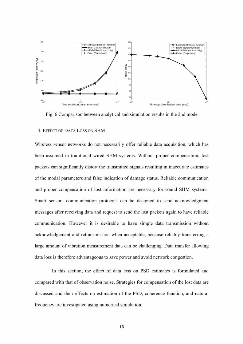
The calculated mode shapes are shown in Fig. 5 and Fig. 6 with respect to the
time synchronization errors. The left figures represent the ratio between the mode shape
amplitudes of the two nodes, and right figures are the phase delay between the two
13

nodes. As expected, phase delay significantly changes as the time synchronization error
increase while the amplitude ratio change is relatively small. For example, nodes 1 and
2 are almost in phase at 0.1 sec synchronization error in Fig. 6; however, the amplitude
ratio is not changed when the input and output are used, or is increased by 2.4% when
only output is used. Note that the higher modes are more sensitive to the
synchronization error because the phase delay depends on the natural frequency. As
shown in Fig. 5 and Fig. 6, the amplitude ratios of the output-only case are affected by
the synchronization error, though it is small, which implies the methods using output
only are more susceptible to the synchronization error.
The impact of the time synchronization error on the identification of the 2DOF
model indicates that the synchronization error distorts significantly the phase
information of the estimated modes. However, smart sensors equipped with appropriate
hardware and time synchronization protocol have been reported to be synchronized
within several milliseconds without significant waste of resources in a system; this level
of the synchronization error may be acceptable in many SHM applications.
10−3
10−2
10−1
1.17
1.18
1.19
1.2
1.21
1.22
1.23
Time synchronization error (sec)
Am
plitu
de r
atio
(y 2
/y1)
Estimated transfer functionExact transfer functionNExT/ERA (Output only)Exact (Output only)
10−3
10−2
10−1
−100
−80
−60
−40
−20
0
20
40
60
80
Time synchronization error (sec)
Pha
se d
elay
Estimated transfer functionExact transfer functionNExT/ERA (Output only)Exact (Output only)
Fig. 5 Comparison between analytical and simulation results in the 1st mode
14
10−3
10−2
10−1
1.68
1.69
1.7
1.71
1.72
1.73
1.74
Time synchronization error (sec)
Am
plitu
de r
atio
(y 2
/y1)
Estimated transfer functionExact transfer functionNExT/ERA (Output only)Exact (Output only)
10
−310
−210
−1
40
60
80
100
120
140
160
180
200
220
Time synchronization error (sec)
Pha
se d
elay
Estimated transfer functionExact transfer functionNExT/ERA (Output only)Exact (Output only)
Fig. 6 Comparison between analytical and simulation results in the 2nd mode
4. EFFECT OF DATA LOSS ON SHM
Wireless sensor networks do not necessarily offer reliable data acquisition, which has
been assumed in traditional wired SHM systems. Without proper compensation, lost
packets can significantly distort the transmitted signals resulting in inaccurate estimates
of the modal parameters and false indication of damage status. Reliable communication
and proper com .
ocols can be designed to send acknowledgment
pensation of lost information are necessary for sound SHM systems
Smart sensors communication prot
messages after receiving data and request to send the lost packets again to have reliable
communication. However it is desirable to have simple data transmission without
acknowledgement and retransmission when acceptable, because reliably transferring a
large amount of vibration measurement data can be challenging. Data transfer allowing
data loss is therefore advantageous to save power and avoid network congestion.
In this section, the effect of data loss on PSD estimates is formulated and
compared with that of observation noise. Strategies for compensation of the lost data are
discussed and their effects on estimation of the PSD, coherence function, and natural
frequency are investigated using numerical simulation.
15

4.1. Compensation approaches
Data loss during wireless communication causes significant errors in subsequent
calculati
ss results in empty space in the
pensate for the lost data is interpolation using data
points around the lost data. “Hold” and “cubic spline” are two major interpolation
methods to consider. In the hold method, the previous data is simply used for the lost
data. The cubic spline method employs the cubic spline fitting to interpolate the lost
data. These two interpolation methods will be considered in an example of SHM
procedure and their performance compared.
centrated in short time duration. Another
method, distributed data packing, in which data in a packet are distributed over the
whole data set, is shown in Fig. 7-(b). These two kinds of packets are considered in this
section.
ons unless appropriately addressed. Measured vibration data in a packet is used
to reconstruct a time history on a receiver node. Time stamps or time indeces in a
received packet correctly specify where in the reconstructed time history the vibration
data in the received packet needs to be expanded. Data lo
reconstructed signal. A way to com
As well as interpolation methods, the method to construct data packets is
considered to have an impact on the subsequent analyses. Since lost information due to
packet loss is determined by how packets are constructed, different packetizing methods
may result in different accuracy of estimated modal parameters. A simple method of
constructing packets, named group packet, is to pack data sequentially, as shown in Fig.
7-(a). When a packet is lost, data loss is con
16

1 11
2
p p
p p
p p
n N n
n n Ny y
+ − +⎛ ⎞⎜ ⎟
⎜ ⎟ ⎜ ⎟⎜ ⎟
⎝ ⎠ ⎝ ⎠⎝ ⎠
2 2 2n N n
y yyy y y
y
+ − +
⎛ ⎞ ⎛ ⎞⎜ ⎟⎜ ⎟
1 2
1 2 2p p pN n N n N n
yy yy y y+ +
⎛ ⎞⎛ ⎞ ⎛ ⎞⎜ ⎟⎜ ⎟ ⎜ ⎟⎜ ⎟⎜ ⎟ ⎜ ⎟
⎜ ⎟⎜ ⎟ ⎜ ⎟⎜ ⎟ ⎜ ⎟ ⎜ ⎟
⎜ ⎟ ⎜ ⎟⎜ ⎟
⎜ ⎟ ⎜ ⎟⎜ ⎟⎜ ⎟ ⎜ ⎟⎜ ⎟ 1 2
p
p p
N n
N N n N N n Ny y y− + − +
⎜ ⎟⎜ ⎟ ⎜ ⎟
⎝ ⎠ ⎝ ⎠ ⎝ ⎠
(a) Group packet data (b) Distributed packet data
Fig. 7 Data packet ( : number of data, : number of data in a packet)
4.2. Effect of data loss on PSD and CSD
In this section, PSD of a signal with the distributed packet data loss is investigated to
obtain an expression of data loss in terms of equivalent observation noise. The PSD is
from the measured data, which is widely
t and output information. Investigation of
N pn
used in calculating the transfer function
employed in modal analysis using the inpu
data loss on PSD estimation will give an insight into its effect on a SHM systems.
Consider a discrete time sequence ( 1, 2, , )ny n N= . ny is assumed as a
stationary random process. For simplicity, the hold method is used to compensate for the
lost data. A total of DN randomly selected data points are assumed to be lost. Subscript
n ( 1, 2, , Di N= ) corresponds to the lost points. The reconstructed signal in the discrete i
time dom
ain can be expressed as
1
D
i
N
n i n n n ni
y ( 1, 2, , )n y A y p n Nδ= + = + =∑ Eq. (13)
re is
−=
whe the difference between niA y and the interpolated value (i.e.,
1i n ni iA y y−= − ), and nδ is the delta functio n is discrete time sequence representing n. p
difference between ny and y . The discrete-time Fourier transform (DFT) of y is
17
given by
1 2exp
N
0k n
n
j knY t y π− −N=
⎡ ⎤= Δ ⎢ ⎥⎣ ⎦∑ Eq. (14)
The PSD of y is
* * * *1 1( )yy k k k k k k k*S f E Y Y Y Y P Y
T T⎡ ⎤ ⎡= = + +⎣ ⎦ ⎣
The DFT of
k k k kY P P P ⎤+ ⎦ Eq. (15)
np * denotes the complex conjugate. is given by
1
2expDN
ik i
i
j knP t ANπ
=
−⎡ ⎤= Δ ⎢ ⎥⎣ ⎦∑ Eq.
nd
(16)
The cross spectral density (CSD) between y a np can be obtained as
* 2
1 1
2 ( )1 1 expD
n
NN
i
Np y k k n in i
j k n nS E P Y E t y AT T
π= =
⎡ ⎤− −⎡ ⎤⎡ ⎤= = Δ⎢ ⎥⎣ ⎦ ⎢ ⎥⎣ ⎦⎣ ⎦ Eq. (17) ∑∑
By taking the expectation of n iy A first,
( )( ) ( )( )( )
( )( ) ( )( )1 1
1
( 1)l N
2 ( )1 exp
21 1 exp
2exp 1
D
n
NNi
p y i in i
ND
Dyy
j k n ntS R n n t R n n tN N
lN j klt R l t R l tN N
N j k SN N
π
π
π
= =
−
− −Δ
N =− −
⎡ ⎤= − + Δ − − Δ ⎢ ⎥⎣ ⎦⎛ ⎞ −⎡ ⎤≅ Δ + Δ − Δ −⎜ ⎟ ⎢ ⎥⎣ ⎦⎝ ⎠
⎛ ⎞⎡ ⎤≅ −⎜ ⎟⎢ ⎥⎣ ⎦⎝ ⎠
∑∑
∑ Eq. (18)
where ( )R t is the autocorrelation function of ny . Using Eq. (16) and assuming that
) is negligible due to the assum on that the lost points are sparse, i jA⎡ ⎤⎣ ⎦ (E A i j≠ pti
18

( )
22
1
2 (0) ( )
D
pp k k k
N
ii
D
Tt E A
Tt N
*1( )S f E P P
R R tN
=
Δ ⎡ ⎤= ⎣ ⎦
Δ ⋅
⎡ ⎤= ⎣ ⎦
= − Δ
∑ Eq. (19)
where is the time step. From Eq. (15), Eq. (18), and Eq. (19), the error in the PSD
estimation defined by
tΔ
yy yy yy⎣ ⎦
S S Sε ⎡ ⎤ = − is
( )2 22cos 1 (S Sε ⎡ ⎤ ≅ − ) (0) ( )D Dyy yy k
N t Nk f R R tN N N
π Δ ⋅⎛ ⎞⎛ ⎞ + − Δ⎜ ⎟⎜ ⎟⎣ ⎦ ⎝ ⎠⎝ ⎠ Eq. (20)
he first term in the right side of Eq. (20) is proportional to and much smT aller than yyS
yyS due to DN N . However, the second term is constant over frequency. This term
ge com yyS at zeros of a system; indeed, yyS is extremely small a
In con
can be lar pared to t
zeros of a system. The overall shape of the PSD is therefore mainly determined by the
second term.
trast to the PSD, the CSD is less susceptible to either data loss or
measurement noise. Since correlation between the data loss terms np
as
oss terms between the signal and data
of two different
signals is small, the cross spectrum of the two data loss can be sumed zero (i.e.,
). Thus, CSD is only affected by the cr
loss, which do not significantly blur zeros of the system. The output-only modal
analysis utilizes CSD mostly and a limited number of PSD at reference points; the
input-output modal analysis requires PSD to obtain each transfer function. The
output-only modal analysis is therefore expected to outperform the methods using both
of input and output with respect to data loss.
1 20p pS =
19
Comparison of the second term with the error in the PSD estimation induced by
the observation noise reveals the data loss level in terms of the noise level. Consider the
white noise with the standard deviation nσ . The PSD of the noise is constant in the
frequency domain and represented as 2n tσ ⋅Δ . An equation to relate the observation
noise level with the data loss level in Eq. (19) can be written as follows.
( ) 22 Dt N R (0) ( ) nR t tN
σΔ ⋅− Δ = ⋅Δ Eq. (21)
Let the RMS noise level and the data loss level be and dρnρ , respectively.
# of lost data
# of data
nn
σ
y
n
ρ
ρ
=
=
Eq. (22)
here
σ
is the standard deviation of nyw yσ . Eq. (21)
is then simplified as
2
( )1d
2(0)
n
R t⎛ ⎞Δ−⎜ ⎟R
ρρ =
⎝ ⎠
Eq. (23)
ata loss is shown to have similar effect on PSD as
derived analytically here, Eq. (23) is expected to hold for subsequent analyses, i.e.,
to investigate the effects of data
loss on the procedure of the SHM. The selected model is a 53DOF statically determinate
D observation noise. Though not
modal analysis and damage detection. This conjecture, as well as the effect of
packetizing, is investigated with numerical simulation.
4.3. Example
A computer simulation is conducted for a truss model
20

structure as shown in Fig. 8. Each element has a Young’s modulus of 200GPa and
cross-sectional area of 112.2m2. The truss is vertically excited at node 6 with the
band-limited white noise, and the vertical accelerations of the bottom nodes (node 2~14)
are measured. After data is acquired at the sampling frequency of 380 Hz, a certain
percentage of packets are randomly dropped to simulate data loss. Two ways of data
loss, group and distributed packet data, are applied to the simulated acceleration of the
planar truss model. In this simulation, the size of packet is selected to be 8. The lost
points are selected randomly, and the hold and cubic spline methods are used to
interpolate lost data. ERA is employed in modal analysis. Each simulation is repeated
100 times and averaged. The simulation results are shown in Fig. 11 and Fig. 12.
Fig. 8 Planar truss model
To verify Eq. (23), the outcome is compared to that of the computer simulation
including observation noise (but without data loss). A band-limited white noise is added
to each of the observed signals pecified as a percentage of the
RMS of
. The RMS noise level is s
physical response. Data loss level of 0.38% is estimated from Eq. (23) to have
similar effects on power spectral density as observation noise of 5%. Fig. 9 shows both
of data loss and noise result in the same effect on the PSD and coherence function.
21

0 20 40 60 80 100 120 140 160 18010
−7
10−6
10−5
10−4
10−3
10−2
10−1
100
101
Frequency (Hz)
Pow
er s
pect
ral d
ensi
ty
IdealData loss 0.38%Noise 5%
0 20 40 60 80 100 120 140 160 1800
0.1
0.2
0.3
0.4
0.5
0.6
0.7
0.8
0.9
1
Frequency (Hz)
Coh
eren
ce
Fig. 9 Data loss effect on power spectral density and coherence at node 10
0 20 40 60 80 100 120 140 160 18010
−7
10−6
10−5
10−4
10−3
10−2
10−1
100
101
Frequency (Hz)
Cro
ss s
pect
ral d
ensi
ty
IdealData loss 0.38%Noise 5%
Fig. 10 Data loss effect on cross spectral density between node 8 and 10
The loss of data reduces the coherence function except at the system's poles (see Fig. 9).
Because of the random nature of data loss occurrence and the excitation, the coherence
function varies from simulation to simulation. In FFT calculations, twenty averages are
used. The coherence function's deviation from unity depends on the input and output,
between which the function is calculated. All the investigated coherence function plots,
however, support 10 % noise addition affects the coherence function in a similar way as
the loss of 0.5~ 2.5 % data does, which agrees with what Eq. (23) suggests for PSD.
The zeros of the estimated CSDs of accelerations at node 8 and 10 remain clear
22
with either data loss or measurement noise (See Fig. 10). Although there is some
difference at the zeros, both data loss and measurement noise do not distort the CSD
significantly as compared to the PSD plot in Fig. 9. Randomness of data loss and noise
makes , resulting in an accurate estimation of the CSD. Note that the two
CSDs with data loss and measurement noise are close to each other, which implies
1 20p pS =
Eq. (23) still hold for CSD estimation and modal analysis using output only.
Fig. 11 and Fig. 12 illustrate the errors in the estimated natural frequencies
under the various levels of data loss. The errors are calculated with respect to the
estimated natural frequencies without any data loss. These figures reveal the cubic
spline method does not give a significant benefit in spite of the additional computation
required. When the hold method is used, both of the group and distributed packets
provide a similar level of accuracy overall. However, the effect of these two packetizing
methods on the damage detection algorithm employed in a SHM system should be
investigated before selecting one of them. In addition, the modal analysis methods using
only output information are found more robust against both of data loss and noise by
comparing Fig. 11 and Fig. 12. The mean and standard deviation of the error are
significantly reduced in Fig. 12, which agrees with the small errors in estimation of
CSD with data loss and noise.
The relationship between noise and data loss, Eq. (23), can be verified to hold
for modal analysis in Fig. 11 and Fig. 12. The distributed packet and hold method are
assumed when Eq. (23) is obtained in the previous section. The estimated natural
frequencies from the distributed packet and hold methods exhibit close error mean and
standard deviation to those of the noise case in Fig. 11 and Fig. 12. The mean error
23

in Fig. 12 are difficult to distinguish; however, if zoomed in, they are close.
Particularly Fig. 12 indicates that Eq. (23) works for the methods using output only as
expected from CSD estimation.
In this example, the effect of data loss on the SHM system is discussed. The
PSD estimates from the simulated data validate Eq. (23), the relationship between data
loss and observation noise level. Even though not verified analytically, Eq. (23) appears
to hold for other function estimates and the subsequent analysis results, such as CSD,
coherence, and the natural frequency estimation. The hold method with either group or
distributed packet is recommended in a SHM system allowing small amounts of data
loss.
0 0.5 1 1.5 2 2.5 3−0.04
−0.02
0
0.02
0.04
0.06
0.08
1st Natural Frequency(Hz)
μ err
or (
%)
Group Loss (Hold)Group Loss (Spline)Distr. Loss (Hold)Distr. Loss (Spline)Noise
0 0.5 1 1.5 2 2.5 30
0.01
0.02
0.03
0.04
0.05
0.06
σ err
or (
%)
Data Loss (%)
Group Loss (Hold)Group Loss (Spline)Distr. Loss (Hold)Distr. Loss (Spline)Noise
0 0.5 1 1.5 2 2.5 3−0.04
−0.02
0
0.02
0.04
0.06
0.08
4th Natural Frequency(Hz)
μ err
or (
%)
Group Loss (Hold)Group Loss (Spline)Distr. Loss (Hold)Distr. Loss (Spline)Noise
0 0.5 1 1.5 2 2.5 30
0.01
0.02
0.03
0.04
0.05
0.06
σ err
or (
%)
Data Loss (%)
Group Loss (Hold)Group Loss (Spline)Distr. Loss (Hold)Distr. Loss (Spline)Noise
Fig. 11 Errors of estimated natural frequencies when input and output are used
24

0 0.5 1 1.5 2 2.5 3−2
−1
0
1
2
3
4
x 10−3 1st Natural Frequency(Hz)
μ err
or (
%)
Group Loss (Hold)Group Loss (Spline)Distr. Loss (Hold)Distr. Loss (Spline)Noise
0 0.5 1 1.5 2 2.5 30
0.01
0.02
0.03
0.04
0.05
0.06
σ err
or (
%)
Data Loss (%)
Group Loss (Hold)Group Loss (Spline)Distr. Loss (Hold)Distr. Loss (Spline)Noise
0 0.5 1 1.5 2 2.5 3−2
−1
0
1
2
3
4
x 10−3 4th Natural Frequency(Hz)
μ err
or (
%)
Group Loss (Hold)Group Loss (Spline)Distr. Loss (Hold)Distr. Loss (Spline)Noise
0 0.5 1 1.5 2 2.5 30
0.01
0.02
0.03
0.04
0.05
0.06
σ err
or (
%)
Data Loss (%)
Group Loss (Hold)Group Loss (Spline)Distr. Loss (Hold)Distr. Loss (Spline)Noise
Fig. 12 Errors of estimated natural frequencies when only output is used
5. COORDINATED COMPUTING
The amount of data involved in SHM applications normally exceeds practical
communication capabilities of smart sensor networks if all the measurement data needs
to be collected centrally; data aggregation has been an important issue to be addressed
before a SHM system employing smart sensors is realized. One approach to overcome
this data aggregation problem has been an independent data processing strategy. This
approach, however, cannot fully exploit information available in the sensor network.
Distribution of data processing and coordination among smart sensors play central roles
in addressing many smart sensor implementation issues, including data aggregation.
This section will demonstrate that distribution and coordination can be well planned so
that the data aggregation problem is addressed without sacrificing structural analysis
performance. Two examples of distributed computing based on SHM analyses are
provided to illustrate the approach.
5.1. Distributed implementation of correlation function estimation
Correlation function estimation is oftentimes the beginning step of output-only SHM of
25

civil infrastructure and usually involves a large amount of measurement data (Gao
2005). Cross-correlation estimation needs data from two sensor nodes. Measured data
needs to be transmitted from one node to the other before the processing takes place.
Associated data communication can be prohibitively large without careful consideration
for implementation. Distribution of data processing and coordination among smart
sensors are addressed herein to incorporate application specific knowledge into data
aggregation.
Correlation functions are, in practice, estimated from finite length records.
Power and cross spectral density (PSD/CSD) functions are estimated first through the
following relation (Bendat and Piersol 2000):
*
1
1( ) ( ) ( )dn
xy i iid
G Xn T
Yω ω ω=
= ∑ Eq. (24)
where ( )xyG ω is CSD estimation between two stationary Gaussian random process,
( )x t and ( )y t . ( )X ω and ( )Y ω are the Fourier transform of ( )x t and ( )y t ; the *
denotes the complex conjugate. T is time length of sample records, ( )ix t and ( )iy t .
When , the estimate has a large random error. The random error is reduced by
computing an ensemble of the estimates from different or partially overlapped
records. The normalized RMS error
1dn =
dn
( )xyGε ω⎡ ⎤⎣ ⎦ of the spectral density function
estimation is given as
1( )xyxy d
Gn
ε ωγ
⎡ ⎤ =⎣ ⎦ Eq. (25)
xyγ is the coherence function between ( )x t and ( )y t , indicating the degree of
26

linearity between them. Through the averaging process, the estimation error is reduced.
Averaging of 10-20 times is common practice. The estimated spectral densities are then
converted to correlation functions by inverse Fourier transform.
An implementation of correlation function estimation for a small community of
sensors in a centralized data collection scheme is shown in Fig. 13. where node 1 works
as a reference sensor. Assuming sn nodes, including the reference node, are measuring
structural response, each node acquires data and sends to the reference node. The
reference node calculates the spectral density as in Eq. (24). This procedure is repeated
times and averaged. After averaging, the inverse FFT is taken to calculate the
correlation function. All the calculation takes place at the reference nodes. When the
spectral density is estimated from discrete time history records of length , data to be
transmitted through the radio is
dn
N
( 1)d sN n n× × − .
Node 1x1
Node 2x2
Node 3x3
Node 4x4
Node nsxns
. . .Node 4x4
( ) ( )1 iE x t x t τ+⎡ ⎤⎣ ⎦i =1,2,…,ns
Node 1x1
Node 2x2
Node 3x3
Node 4x4
Node nsxns
. . .Node 4x4
( ) ( )1 iE x t x t τ+⎡ ⎤⎣ ⎦i =1,2,…,ns
Fig. 13 Centralized NExT implementation
In the next scheme, data flow for correlation function estimation is examined and data
transfer is reorganized to take advantage of computational capability on each smart
sensor node. After the first measurement, the reference node broadcasts the time record
to all the nodes. On receiving the record, each node calculates the spectral density
between its own data and the received record. This spectral density estimate is locally
stored. The nodes repeat this procedure times. After each measurement, the stored dn
27

value is updated by taking a weighted average between the stored value and the current
estimate. In this way, Eq. (24) is calculated on each node. Finally the inverse FFT is
applied to the spectral density estimate locally. The resultant correlation function is sent
back to the reference node. Because the subsequent modal analysis such as ERA uses, at
most, half of the correlation function data length, 2N data is sent back to the
reference node from each node. The total data to be transmitted in this scheme is,
therefore, 2 ( 1)dN n N n× + × −s (see Fig. 14).
Node 1x1
Node 2x2
Node 3x3
Node 4x4
Node nsxns
( ) ( )1 2E x t x t τ+⎡ ⎤⎣ ⎦ ( ) ( )1 3E x t x t τ+⎡ ⎤⎣ ⎦ ( ) ( )1 4E x t x t τ+⎡ ⎤⎣ ⎦ ( ) ( )1 snE x t x t τ⎡ ⎤+⎣ ⎦
( ) ( )1 1E x t x t τ+⎡ ⎤⎣ ⎦
. . .Node 4x4
( ) ( )1 4E x t x t τ+⎡ ⎤⎣ ⎦
Node 1x1
Node 2x2
Node 3x3
Node 4x4
Node nsxns
( ) ( )1 2E x t x t τ+⎡ ⎤⎣ ⎦ ( ) ( )1 3E x t x t τ+⎡ ⎤⎣ ⎦ ( ) ( )1 4E x t x t τ+⎡ ⎤⎣ ⎦ ( ) ( )1 snE x t x t τ⎡ ⎤+⎣ ⎦
( ) ( )1 1E x t x t τ+⎡ ⎤⎣ ⎦
. . .Node 4x4
( ) ( )1 4E x t x t τ+⎡ ⎤⎣ ⎦
Fig. 14 Distributed NExT implementation
As the number of nodes increases, the advantage of the second scheme, in
terms of communication requirements, becomes significant. The second approach
requires data transfer of , while the first one needs to transmit to the
reference sensor node data of the size of
(( d sO N n n⋅ + ))
( )d sO N n n⋅ ⋅ . The distributed implementation
leverages knowledge regarding the application to reduce communication requirements
as well as to utilize CPU and memory in a smart sensor network efficiently.
The data communication analysis above assumes that all the nodes are in
single-hop range of the reference node. This assumption is not necessarily the case for a
general SHM application. However, Gao (2005) proposed a Distributed Computing
Strategy (DCS) for SHM which support this idea. Neighboring smart sensors in a
28

single-hop communication range make local sensor communities and perform SHM in
the communities. In such applications, the assumption of nodes being in single hop
range of a reference node is reasonable.
5.2. Distributed Computing Strategy (DCS)
The DCS for SHM proposed by Gao (2005) is suitable for implementation on networks
of densely distributed smart sensors. The conceptual hierarchical organization of the
DCS approach is shown in Fig. 15. In contrast to traditional SHM algorithms which
require all the measured information to be transferred to a central station, the measured
information is aggregated locally by a selected sensor within the sensor group, termed
the manager sensor, and only limited information is sent back to the central station to
provide the condition of the structure. Small numbers of smart sensors are grouped to
form different communities so that all sensors in a community are located in the range
of single hop. Although each sensor in Fig. 15 is included in only one community, in the
DCS approach smart sensors can be contained in multiple communities. Each manager
sensor collects necessary information and implements the damage detection algorithm
for its community. Adjacent manager sensors interact with each other to exchange
information. In Fig. 15, manager sensors in communities 1, 2, and 3 interact with each
other while community 4 does only with community 3. Once information is aggregated,
the manager sensors determine information to be sent back to the central station. The
manager sensor of the community in which damage has not occurred transmits only an
“OK” signal to the central station. If damage has occurred, the manager sensor of the
community needs to send damage information such as damage location, which is
reflected by the solid line in Fig. 15. Thus, the DCS approach requires only limited
29

information need to be transferred between sensors throughout the entire sensor network.
This approach will significantly reduce the communication traffic in the sensor network.
Gao (2005) shows that NExT (James et al. 1992), Eigensystem Realization
Algorithm (Juang and Pappa 1985), and Damage Locating Vector method (Bernal 2002)
can be utilized as structural analysis techniques to materialize this DCS concept. These
structural analyses are applied in each sensor community. The manager sensors
communicate with each other to assess mode shapes’ normalization constants and to
make redundant judgment about damaged element; most of data processing and
communication takes place inside each sensor community. Coordination among smart
sensors employing DCS, which has yet to be implemented, is expected to realize a SHM
system using densely installed smart sensors.
2 3 41CommunitySmart Sensors
manager sensors
Central Station
Fig. 15 Sketch of hierarchical organization
5.3. Implementation on smart sensors
In this section, distributed computing is implemented on a network of smart sensors.
The distributed implementation of correlation function estimation is incorporated into
DCS; correlation function estimation in DCS is conducted in the distributed manner.
Then ERA is applied at a manager sensor to estimate modal parameters. The rest of
30

DCS, i.e, DLV and communication between manager sensors, is currently being
implemented. SHM performance is examined in terms of accuracy of signal processing,
while data aggregation performance is assessed from reduction in communication
requirements during correlation function estimation.
The smart sensor platform used in this demonstration is Imote2. Imote2 has
Intel Xscale processor and 256KB of RAM. Radio components has data rate of 250
Kbps. 256KB of RAM on Imote2 allows implementation of correlation function
estimation from a large amount of data and ERA involving large Hankel and system
matrices. An open source operating system, TinyOS, is utilized to program Imote2s. The
hardware is appropriate for data processing intensive applications such as SHM
To understand the performance of the algorithms, the coordinated computing
implemented on Imote2 is demonstrated using a numerical truss model shown in Fig. 8.
Vertical acceleration responses under random input are measured at nodes 5 to 13 and
injected into a network of nine Imote2s. The Imote2 corresponding to node 5 works as
the reference sensor. This node broadcast its own data to the other node and collect
correlation function estimate. Once all the correlation function estimates are collected,
this reference node applies ERA to obtain natural frequencies, damping ratios and mode
shapes. The length, , of the injected data is 2048 and the number of FFT points is
512, resulting in 7 times averaging with 50 % overlap. The sampling rate is 500 Hz.
N
The acceleration response data and correlation function estimates are stored
and transferred in 16-bit integer data type, considering that accelerometer’s resolution
can be reasonably assumed to be around 12-bit. In this way, memory space and
bandwidth are efficiently utilized, though cast double precision data is used during
31
NExT and ERA.
Although a certain amount of data loss is shown to be acceptable in the
previous section, reliable communication is used in this demonstration. In this way,
outputs of this coordinated computing, i.e., correlation function estimates, natural
frequencies, damping ratios, and mode shapes, are compared with those calculated on a
PC without mixing with the effect of data loss.
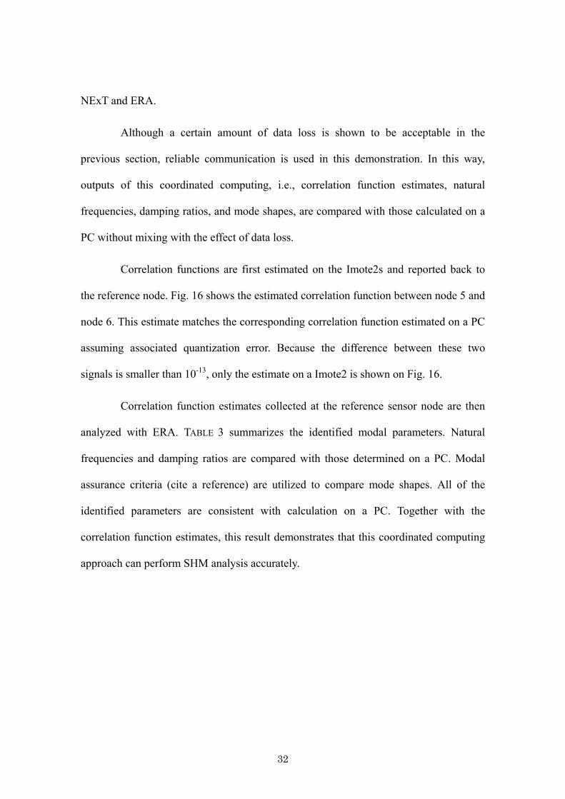
Correlation functions are first estimated on the Imote2s and reported back to
the reference node. Fig. 16 shows the estimated correlation function between node 5 and
node 6. This estimate matches the corresponding correlation function estimated on a PC
assuming associated quantization error. Because the difference between these two
signals is smaller than 10-13, only the estimate on a Imote2 is shown on Fig. 16.
Correlation function estimates collected at the reference sensor node are then
analyzed with ERA. TABLE 3 summarizes the identified modal parameters. Natural
frequencies and damping ratios are compared with those determined on a PC. Modal
assurance criteria (cite a reference) are utilized to compare mode shapes. All of the
identified parameters are consistent with calculation on a PC. Together with the
correlation function estimates, this result demonstrates that this coordinated computing
approach can perform SHM analysis accurately.
32

0.1 0.2 0.3 0.4 0.5−4
−2
0
2
4
0Time (sec)
Cor
rela
tion
func
tion
estim
ate
Fig. 16 A correlation function estimate
Table 3 Results of modal analysis performed on Imote2 Mode 1 2 3 4
Natural Frequency (Hz) 27.21 97.23 127.36 176.14Error(ratio) -2.13E-13 3.26E-13 -3.20E-13 1.71E-13
Damping ratio (%) 4.09 10.35 5.32 0.43Error (ratio) -2.93E-14 1.08E-13 -1.31E-13 1.02E-14
Modal Assurance Criteria of mode shapes - 1
0 -2.22E-16 -2.22E-16 0
Data transferred in a network is reduced as explained in 6.1. In this example,
data transmission is reduced by a factor of 5, as compared to centralized NExT
implementation. This reduction factor can be larger depending on the number of sensors
and the associated averaging. This reduction shows the advantage of distributed
correlation function estimation.
Further consideration is necessary to accurately assess the efficacy of the
distributed implementation. Power consumption of smart sensor networks is not simply
proportional to the amount of data transmitted. Acknowledgement messages and
synchronization messages are also involved. The radio listening mode consumes power
even when no data is received. However, the size of the measured data is usually
much larger than the size of the other messages to be sent and should be considered the
33

primary factor in determining power consumption. Small data transfer requirements will
lead to small power consumption.
6. CONCLUSION
Although smart sensor usage in SHM applications is promising, full-fledged SHM
systems employing smart sensors have not yet been realized. Critical issues such as time
synchronization error, data loss, and a large amount of data have been described and
investigated.
Time synchronization error was formulated and its effects on SHM applications
investigated. Input-output identification and output-only identification were reviewed
with time synchronization error taken into account. Mode shape phase was shown to be
sensitive to time synchronization error. The impact is not negligible when the ratio of
time synchronization error to a natural frequency of a system is large. However, time
synchronization accuracy reasonably available for smart sensors and low natural
frequencies of a large structure oftentimes result in small impact on modal analysis.
Data loss was investigated with respect to the performance of the modal
parameter estimation. An expression was derived relating the amount of data loss to an
equivalent measurement noise. Two types of packet arrangement were considered and
shown to have a similar level of accuracy in most cases. Data loss is found to introduce
error into the modal analysis, which also affects the subsequent analysis. Because of the
averaging associated with the PSD and the CSD estimation, a certain amount of data
loss can be accommodated. Particularly, the CSD estimation is found to be robust
against both of data loss and observation noise, allowing the output-only identification
to be better than the one using input and output.
34

Coordinated computing is shown to be an effective approach for SHM
applications, especially for data aggregation. Two examples of coordinated computing
supported by structural analysis are shown. Implementation on Imote2s demonstrates
the efficacy of this approach.
ACKNOWLEDGEMENTS
This study is supported in part by the National Science Foundation under grant CMS
0301140 (Dr. S. C. Liu, program manager). Partial support from Vodafone, Korea
Science and Engineering Foundation, Kitami Institute of Technology, and Japan
Ministry of Education, Culture, Sports, and Technology is gratefully appreciated. The
support is gratefully acknowledged.
REFERENCES
Arici, Y. and Mosalam, K. M., 2003, “Modal Analysis of a Densely Instrumented
Building Using Strong Motion Data”, Proceedings of the International Conference on
Applications of Statistics and Probability in Civil Engineering, San Francisco, CA, June
6-9, 419-426.
Bendat, J. S. and Piersol, A. G. (2000), Random data: analysis and measurement
procedures, John Wiley and Sons, Inc. New York, NY.
Bernal, D. (2000), “Extracting flexibility matrices from state-space realization.”, COST
F3 Conf., Madrid, Spain, 127-135.
Bernal, D. (2002), “Load vectors for damage localization”, Journal of Engrg. Mech.,
128(1):7-14.
Casciati, F., Faraveli, L. and Borghetti, F., 2003, “Wireless Links between
35

Sensor-Device Control Stations in Long Span Bridges”, Smart Structures and Materials
2003: Smart Systems and Nondestructive Evaluation for Civil Infrastructures,
Proceedings of the SPIE, Vol. 5057, San Diego, CA, pp. 1-7
Celebi, M. (2002), “Seismic instrumentation of buildings (with emphasis on federal
buildings)” Special GSA/USGS Project, an administrative report, United States
Geological Survey, Menlo Park, CA.
Crossbow Technology, Inc. http://www.xbow.com
Doebling, S. W., Farrar, C. R., Prime, M. B., and Shevitz, D. W. (1996), “Damage
identification and health monitoring of structural and mechanical systems from changes
in their vibration characteristics: a literature review”, LA-13070-MS.
Doebling, S. W., Farrar, C. R., and Prime, M. B. (1998), “A summary review of
vibration-based damage identification methods”, The Shock and Vibration Digest, vol.
30, no. 2, pp. 91-105.
Doebling, S. W. and Farrar, C. R. (1999), “The state of the art in structural identification
of constructed facilities”, A report by American Society of Civil Engineers Committee on
Structural Identification of Constructed Facilities.
Elson, J., Girod, L. and Estrin, D. (2002), “Fine-Grained Network Time
Synchronization using Reference Broadcasts”, Proc. of the Fifth Symposium on
Operating Systems Design and Implementation (OSDI 2002).
Farrar, C. R. (2001), “Historical overview of structural health monitoring”, Lecture
Notes on Structural Health Monitoring using Statistical Pattern Recognition, Los
Alamos Dynamics, Los Alamos, NM.
36

Gao., Y. (2005), “Structural health monitoring strategies for smart sensor networks.”
PhD Dissertation, University of Illinois at Urbana-Champaign.
Gros, X. E. (1997), NDT data fusion, Arnold, London, UK.
Hollar, S. (2000), COTS Dust., Master's Thesis, University of California, Berkeley, CA.
James, G. H., Carne, T. G., and Lauffer, J. P. (1993), “The natural excitation technique
for modal parameter extraction from operating wind turbine”, Report No.
SAND92-1666, UC-261, Sandia National Laboratories, Sandia, NM..
James, G. H., Carne, T. G., Lauffer, J. P., and Nord, A. R. (1992), “Modal testing using
natural excitation”, Proceedings of 10th Int. Modal Analysis Conference, San Diego, CA.
Kottapalli, V. A., Kiremidjian, A. S., Lynch, J. P., Carryer, E., Kenny, T. W., Law, K. H.,
and Lei, Y., 2003, “Two-tiered Wireless Sensor Network Architecture for Structural
Health Monitoring”, in Smart Structures and Materials, San Diego, CA, March 3-6,
Proceedings of the SPIE, Vol. 5057, 8-19.
Kurata, N., Spencer, B. F. Jr., and Ruiz-Sandoval, M., 2004, “Building Risk Monitoring
Using Wireless Sensor Network”, Proceedings of the 13th World Conference on
Earthquake Engineering, August 2-6, Vancouver, BC, Cananda.
Lei, Y., Kiremidjian, S., Nair, K.K., Lynch, J.P. and Law, K.H. (2004), “Algorithms for
time synchronization of wireless structural monitoring sensors”, Earthquake Engng
Struct. Dyn., 34:555-573.
Lyncn, J. P., Wang, Y., Law, K. H., Yi, J.-H., Lee, C. G., Yun, C. B. (2005), “Validation
of a large-scale wireless structural monitoring system on the Geumdang bridge.”,
Proceedings of the Int. Conference on Safety and Structural Reliability, Rome, Italy
37

Lynch, J. P. and Loh, K. J. (2006), "A summary review of wireless sensors and sensor
networks for structural health monitoring”, Shock and Vibration Digest, 38(2), 91-128.
Mechitov, K., Kim, W., Agha, G., and Nagayama, T. (2004), “High-frequency
distributed sensing for structure monitoring”, Proceedings of 1st Int. Workshop on
Networked Sensing Systems, 101-105
Nagayama, T., Ruiz-Sandoval, M., Spencer Jr., B. F., Mechitov, K. A., Agha, G.. A.
(2004), “Wireless strain sensor development for civil infrastructure”, Proceedings of 1st
Int. Workshop on Networked Sensing Systems, Tokyo, Japan, 97-100.
Nagayama, T., Abe, M., Fujino, Y. And Ikeda, K. (2005), “Structural Identification of a
Nonproportionally Damped System and Its Application to a Full-Scale Suspension
Bridge”, Journal of Structural Engineering, Vol. 131, No. 10, 1536-1545.
Nagayama, T., Spencer, Jr., B. F., Agha, G. A., and Mechitov, K. A. (2006),
"Model-based data aggregation for structural monitoring employing smart sensors",
Proceedings of the Third International Conference on Networked Sensing Systems (INSS
2006), May 31- Jun 2, pp. 203-210.
Nitta, Y., Nagayama, T., Spencer Jr., B. F., and Nishitani, A. (2005), “Rapid damage
assessment for the structures utilizing smart sensor MICA2 MOTE”, Proceedings of 5th
Int. Workshop on Structural Health Monitoring, Stanford, CA., 283-290
Salawu, O. S. and Williams, C. (1995), “Review of full-scale dynamic testing of bridge
structures”, Engineering Structures, vol. 17, no. 2, pp. 113-121.
Sohn, H., Farrar, C. R., Hemez, F. M., Shunk, D. D., Stinemates, D. W., and Nadler, B.
R. (2001), “A review of structural health monitoring literature: 1996-2001”, Los Alamos
38

39
National Laboratory Report, LA-13976-MS.
Spencer Jr., B. F., Ruiz-Sandval, M. E. and Kurata, N. (2004), “Smart sensing
technology: opportunities and challenges”, Structural Control and Health Monitoring,
11:349-368.
Ruiz-Sandoval, M. (2004), “Smart sensors for civil infrastructure systems”, Ph.D.
Dissertation, University of Notre Dame, IN.
Ruiz-Sandoval, M., Nagayama, T., and Spencer, B.F. (2006), "Sensor development
using Berkeley Mote platform", Journal of Earthquake Engineering, 10(2), 289-309.
Wang, Y., Lynch, J. P., and Law, K. H. (2005), “Wireless Structural Sensors Using
Reliable Communication Protocols for Data Acquisition and Interrogation”,
Proceedings of the 23rd International Modal Analysis Conference (IMAC XXIII),
Orlando, FL, January 31-February 3.
Wong, K. Y. (2004), “Instrumentation and health monitoring of cable-supported
bridges”, Structural Control and Health Monitoring, 11(2), 91-124