isterre / cnrs / universit e grenoble alpes · cool facts about the earth’s core a broad range of...

Turbulence in geodynamo simulations

Nathanael Schaeffer, A. Fournier, D. Jault, J. Aubert, H-C. Nataf, ...

ISTerre / CNRS / Universite Grenoble Alpes

Journee des utilisateurs CIMENT, Grenoble, 23 June 2016

[email protected] (ISTerre) Earth’s core simulations CIMENT 23 June 2016 1 / 29

Outline

1 Introduction

2 The XSHELLS codeEquationsThe SHTns libraryParallelization strategy and tricks

3 Turbulence in geodynamo simulations


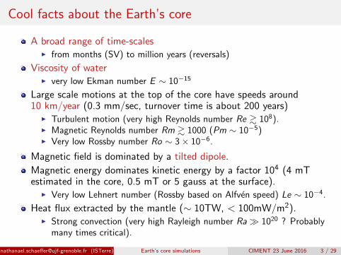
Cool facts about the Earth’s core

A broad range of time-scalesI from months (SV) to million years (reversals)

Viscosity of waterI very low Ekman number E ∼ 10−15

Large scale motions at the top of the core have speeds around10 km/year (0.3 mm/sec, turnover time is about 200 years)

I Turbulent motion (very high Reynolds number Re & 108).I Magnetic Reynolds number Rm & 1000 (Pm ∼ 10−5)I Very low Rossby number Ro ∼ 3× 10−6.

Magnetic field is dominated by a tilted dipole.

Magnetic energy dominates kinetic energy by a factor 104 (4 mTestimated in the core, 0.5 mT or 5 gauss at the surface).

I Very low Lehnert number (Rossby based on Alfven speed) Le ∼ 10−4.

Heat flux extracted by the mantle (∼ 10TW, < 100mW/m2).I Strong convection (very high Rayleigh number Ra 1020 ? Probably

many times critical).


Broad questions

Turbulence: does it matter? How?I What do the flow and magnetic field look like?I What are the basic equilibriums?I Can we build a reduced model?

Observations: short time-scales (a few years)I Importance of waves?I Length-of-day variations?I Effect of a stable ocean at the top of the core?


Basic rotating MHD in planetary cores

Navier-Stokes equation

∂tu + (2Ω ez +∇× u)× u = −∇p + ν∆u+ (∇× b)× b − αg T ~r

Induction equation

∂tb = ∇× (u× b) +η∆b

Temperature equation

∂tT + u.∇T = κ∆T

E = ν/D2Ω ∼ 10−15

Pm = νµ0σ ∼ 10−5Ra = ∆TαgD3/κν 1 (?)

Pr = ν/κ ∼ 1


Outline

1 Introduction

2 The XSHELLS codeEquationsThe SHTns libraryParallelization strategy and tricks



MHD forced by Boussinesq convection

XSHELLS time-steps the following equations:

∂tu + (2Ω0 +∇× u)× u = −∇p∗ + ν∆u + (∇× b)× b + c∇Φ0

∂tb = ∇× (u× b) + η∆b

∂tc + u.∇(c + C0) = κ∆c

∇u = 0 ∇.b = 0

Spherical shell geometry

Fields expanded using u = ∇× (T r) +∇×∇× (Pr)

Spherical Harmonic expansion, with transforms done by SHTns

Finite differences in radius

Semi-implicit scheme: diffusive terms are implicit, while other termsare treated explicitly.


Why Spherical Harmonics transform ?

The goal was to use spherical harmonics to time-step Navier-Stokes andrelated equations in spherical geometry.

Pros

Advantage of spectral methods

Don’t need to solve for magnetic field in the insulator.

Strongly reduces the number of variables to solve for.

Cons

No working fast transform: O(N3) for N2 degrees of freedom.

Non-local (more difficult to parallelize)

Spherical Harmonics Transform (SHT) is the bottleneck


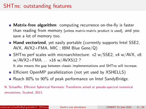
SHTns: outstanding features

Matrix-free algorithm: computing recurrence on-the-fly is fasterthan reading from memory [unless matrix-matrix product is used], and yousave a lot of memory too.

Hand vectorized, yet easily portable (currently supports Intel SSE2,AVX, AVX2+FMA, MIC ; IBM Blue Gene/Q)

SHTns perf scales with microarchitecture: x2 w/SSE2, x4 w/AVX, x8w/AVX2+FMA. . . x16 w/AVX512 ?It also means the gap between classic implementations and SHTns will increase.

Efficient OpenMP parallelization (not yet used by XSHELLS)

Reach 80% to 90% of peak performance on Intel SandyBridge.

N. Schaeffer, Efficient Spherical Harmonic Transforms aimed at pseudo-spectral numerical

simulations, Gcubed, 2013.


SHTns: other interesting features

both scalar and vector transforms.

accurate up to spherical harmonic degree ` = 16383 (at least).

SHT at fixed m (without fft, aka Legendre transform).

spatial data can be stored in latitude-major or longitude-major arrays.

various normalization conventions.

can be used from Fortran, c/c++, and Python programs.

free software : https://bitbucket.org/nschaeff/shtns


https://bitbucket.org/nschaeff/shtns

Parallelization strategy

hybrid MPI/OpenMP parallelization

Increase Data Locality: work shell by shell for spatial terms (do notcompute the whole spatial fields at once: lower memory required andfaster).

Distribute shells to MPI processes (at least 1 shell/process).

No transposition required (no MPI Alltoall()), communicationwith nearest neighbor only.

Use OpenMP within these processes (tested up to 32 threads/shell)

good scaling (e.g. 2688 x 1344 x 1152 @ 6912 cores : 0.8 sec/step onOccigen)


Strategy – non-linear terms

Design choice: optimize the computation of non-linear terms first.

Trick 1: Use SHTns

J. Aubert plugged SHTns into Parody and observed a performanceincrease by a factor of about 2 for the whole code.⇒ lower memory required, faster, ready for future architectures.

Trick 2: Increase Data Locality

Work shell by shell when computing spatial terms (do not compute thewhole spatial fields at once).⇒ lower memory required and significantly faster.


Strategy – linear solver

The linear solver is computationally very cheap. It should deal with thedata as it is arranged for the non-linear terms to be most efficient.

Trick 3: Avoid transpositions and large copies

Transposition is always slow (with and without MPI communications)

Copying large amounts of data can also be quite slow.

Problem: the forward (backward) substitutions depend on the datacomputed by previous (next) processes.


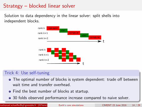
Strategy – blocked linear solver

Solution to data dependency in the linear solver: split shells intoindependent blocks.

t

t

rank k

rank k+1

rank k+2

rank k

rank k+1

rank k+2

compute

compute

compute

xfer

xfer

Trick 4: Use self-tuning

The optimal number of blocks is system dependent: trade off betweenwait time and transfer overhead.

Find the best number of blocks at startup.

30 folds observed performance increase compared to naive solver.


Summary: spherical MHD simulations with XSHELLS

Spherical harmonics,

finite differences (radial),

versatile,

very efficient even on yourlaptop,

OpenMP and/or MPIparallelization with goodscaling,

open source, with usermanual.

101 102 103 104

number of cores

10-1

100

101

102

seco

nds

per

itera

tion

Performance scaling of xshells (NR=512, Lmax=511)

Froggy (SandyBridge) radial OpenMP

Froggy (SandyBridge) in-shell OpenMP

Turing (Blue Gene/Q) in-shell OpenMP

Figure 1: Strong scaling of XSHELLS withspatial resolution Nr = 512, Lmax = 511.

https://bitbucket.org/nschaeff/xshells


https://bitbucket.org/nschaeff/xshells

Outline

1 Introduction

2 The XSHELLS code



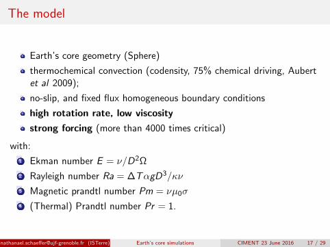
The model

Earth’s core geometry (Sphere)

thermochemical convection (codensity, 75% chemical driving, Aubertet al 2009);

no-slip, and fixed flux homogeneous boundary conditions

high rotation rate, low viscosity

strong forcing (more than 4000 times critical)

with:

1 Ekman number E = ν/D2Ω

2 Rayleigh number Ra = ∆TαgD3/κν

3 Magnetic prandtl number Pm = νµ0σ

4 (Thermal) Prandtl number Pr = 1.


The simulations

The idea

Keep super-criticality and Rm = UD/η ' 650 fixed.

go to more Earth-like A = U/B and Pm = ν/η.

10-5 10-4 10-3 10-2 10-1 100 101

Pm

10-2

10-1

100

101

A

Earth

Soderlund et. al. 2012

Christensen & Aubert 2006

Andrey Sheyko 2014

Other simulations

Highway

initial: E = 10−5,Pm = 0.4, Ra = 6 1010

⇒ A = 1.5 Fν = 47%

jump 1: E = 10−6,Pm = 0.2, Ra = 1.2 1012

⇒ A = 0.61 Fν = 24%

jump 2: E = 10−7,Pm = 0.1, Ra = 2.4 1013

⇒ A = 0.45 Fν = 17%

Extreme parameters, require 2688 x 1344 x 1024 points (3.7 billions)7 months computation on 512 cores (10.5 sec/step)


Energy vs Time

0 2000 4000 6000 8000 10000 12000t=2¼

107

108

109

energ

y

jump 1

jump 2

S0: E=10¡5 Pm=0: 4

S1: E=10¡6 Pm=0: 2

S2: E=10¡7 Pm=0: 1

S1*: E=10¡6 Pm=0

Jump 2 ran for 1.5% of a magnetic diffusion time, and it took about 7 months to

compute on 512 cores, spending 2.5 million core hours.


Snapshot: initial Uφ (E = 10−5, Pm = 0.4, A = 1.5)

NR = 224, Lmax = [email protected] (ISTerre) Earth’s core simulations CIMENT 23 June 2016 20 / 29

Snapshot: jump 1 Uφ (E = 10−6, Pm = 0.2, A = 0.62)


Snapshot: jump 2 Uφ (E = 10−7, Pm = 0.1, A = 0.43)


Jump 2: Temperature field

Mean temperature of each shell has been removed.


Averages of U and B

U

B


Jump 2: Non-zonal mean flow

Homegeneous heat flux start to produce large scale flows at E = 10−7


Jump 2: Space-time Fourier analysis

Fourier Transform in the two homogeneous directions: t and φ.Two different regions inside and outside the tangent cylinder.E = 10−7, Pm = 0.1


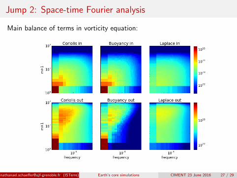
Jump 2: Space-time Fourier analysis

Main balance of terms in vorticity equation:


Jump 1: Influence of the magnetic field

0.470 0.475 0.480 0.485 0.490 0.495time (viscous)

0

1

2

3

4

5

6

7

energ

y

1e8

Ek, step1

Em, step1

Ek, no B

Figure 2: Energies as a function of time (normalized by the viscous diffusion time)for case jump 1 (E = 10−6) and for the same parameters as jump 1, but withoutmagnetic field.


Jump 1: Influence of the magnetic field

With a strong dynamo magnetic field:

Zonal jets are suppressed, plumes extend further.

Larger plumes...

... but convection still starts at small length-scale ! (E 1/3).


Some numbers

definition initial jump 1 jump 2 Earth’s coreNr 224 512 1024Lmax 191 479 893Ek ν/D2Ω 10−5 10−6 10−7 3 10−15

Ra ∆TαgD3/κν 6 1010 1.2 1012 2.4 1013 1030 ?Pm ν/η 0.4 0.2 0.1 3 10−5

Pr ν/κ 1 1 1 0.1 - 10Rm UD/η 710 660 585 2000 ?A

√µρU/B 1.48 0.62 0.43 0.01

Re UD/ν 1770 3300 5850 2 108

Ro U/DΩ 0.018 3.3 10−3 5.9 10−4 3 10−6

Le B/√µρDΩ 0.012 5.3 10−3 1.35 10−3 10−4

Λ B2/ηΩ 5.8 5.7 1.8 1 - 10Fν Dν/(Dη + Dν) 47% 24% 17% ?Fη Dη/(Dη + Dν) 53% 76% 83% ?

Table 1: Various input and output parameters of our simulations, where D is theshell thickness, U the rms velocity and B the rms magnetic field.


Jump 2: spectra

100 101 102

`/r

103

104

105

106

107

108

Ek deep

Ek surface

Em deep

Em surface

E = 10−7

Pm = 0.1Ra = 2.4 1013

Rm = 600A = 0.45Λ = 1.2Fν = 17%

NR = 1024Lmax = 893

Magnetic field dominates deep in the core but not near the surface.

Velocity spectrum nearly flat at the surface but increasing deep down.


Jump 2: z-averaged energy densities

z-averaged equatorial energy densities, left: < U2eq >, right: < B2

eq >.E = 10−7, Pm = 0.1, Rm = 600, A ∼ 0.45.


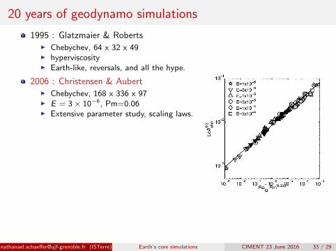
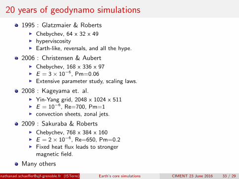
20 years of geodynamo simulations

1995 : Glatzmaier & RobertsI Chebychev, 64 x 32 x 49I hyperviscosityI Earth-like, reversals, and all the hype.

2006 : Christensen & AubertI Chebychev, 168 x 336 x 97I E = 3 × 10−6, Pm=0.06I Extensive parameter study, scaling laws.

2008 : Kageyama et. al.I Yin-Yang grid, 2048 x 1024 x 511I E = 10−6, Re=700, Pm=1I convection sheets, zonal jets.

2009 : Sakuraba & RobertsI Chebychev, 768 x 384 x 160I E = 2 × 10−6, Re=650, Pm=0.2I Fixed heat flux leads to stronger

magnetic field.

Many others


isterre / cnrs / universit e grenoble alpes · cool facts about the earth’s core a broad range of...

Documents