it’s all about volatility (of volatility): evidence from...

Department of Economics and Business

Aarhus University

Fuglesangs Allé 4

DK-8210 Aarhus V

Denmark

Email: [email protected]

Tel: +45 8716 5515

It’s all about volatility (of volatility): evidence from a two-

factor stochastic volatility model

Stefano Grassi and Paolo Santucci de Magistris

CREATES Research Paper 2013-03

It’s all about volatility (of volatility):

evidence from a two-factor stochastic volatility model ∗

Stefano Grassi† Paolo Santucci de Magistris‡

March 11, 2013

Abstract

The persistent nature of equity volatility is investigated by means of a multi-factorstochastic volatility model with time varying parameters. The parameters are estimatedby means of a sequential indirect inference procedure which adopts as auxiliary model atime-varying generalization of the HAR model for the realized volatility series. It emergesthat during the recent financial crisis the relative weight of the daily component dominatesover the monthly term. The estimates of the two factor stochastic volatility model suggestthat the change in the dynamic structure of the realized volatility during the financial crisisis due to the increase in the volatility of the persistent volatility term. As a consequence ofthe dynamics in the stochastic volatility parameters, the shape and curvature of the volatilitysmile evolve trough time.

Keywords: Time-Varying Parameters, On-line Kalman Filter, Simulation-based inference,Predictive Likelihood, Volatility Factors.

JEL Classification:G01, C00, C11, C58

∗The authors are grateful to CREATES - Center for Research in Econometric Analysis of Time Series(DNRF78), funded by the Danish National Research Foundation.

†Aarhus University and CREATES, Department of Economics and Business, Fuglsang Alle 4; DK-8210 AarhusV, Denmark; phone: +45 8716 5319; email address: [email protected].

‡Aarhus University and CREATES Department of Economics and Business, Fuglsang Alle 4; DK-8210 AarhusV, Denmark; phone: +45 8716 5319; email address: [email protected]

1

1 Introduction

The aim of this paper is to evaluate whether the observed changes in the dynamic behavior of

the realized volatility (RV) series, in correspondence to the financial crises, are linked to changes

in the structural parameters governing the stochastic volatility (SV) dynamics. In other words

the observed changes in the dynamic pattern of RV series during the financial crises may be seen

as the outcome of structural breaks in the parameters governing the dynamics of the continuous-

time SV process. For this purpose, a two factors SV model (TFSV) is chosen as structural model,

since, as noted by Gallant et al. (1999) and Meddahi (2002, 2003), it successfully accounts for

the long range dependence of the volatility process. Given the difficulty of a direct estimation

of breaks in the TFSV parameters, we adapt the indirect inference procedure suggested by

Corsi and Reno (2012) to the case in which the SV parameters are allowed to be recursively

updated. We therefore propose a sequential indirect inference approach, exploiting a flexible

specification for the auxiliary model, which is built on an ex-post measure of the integrated

variance. The auxiliary model is a simple time varying extension of the well-known HAR model

of Corsi (2009), and it represents a tool to evaluate to what extent the parameters governing

the dynamic structure of the RV process vary over time. The time-varying HAR (TV-HAR) is

interesting per se since it constitutes a tool to evaluate the evolution of the relative weight of each

volatility component to the overall volatility persistence. Following Raftery et al. (2010) and

Koop and Korobilis (2012), we use a fast on-line method to extract the TV-HAR parameters,

allowing for a rapid update of the estimates as each new piece of information arrives. The

advantage of the proposed estimation method is that it does not require to identify the number

of change points and avoids the use of computationally intensive algorithms, such as MCMC.

The empirical analysis is carried out on the RV series of 15 assets traded on the NYSE, which

are supposed to be representative of the main sectors of the US economy. The estimates of the

TFSV model indicate that the change in persistence is due to the increase of the relative weight of

the persistent volatility component during the financial crisis. In particular, the volatility of the

persistent factor increases relatively to that of the non-persistent factor, generating trajectories

that deviate for longer periods from the unconditional mean. This may generate the impression

of level shifts in the observed realized series. However the model selection procedure, based on

the predictive likelihood, excludes that breaks in the long-run mean during the financial crises

are responsible for the increase in the observed persistence of the volatility series. Moreover, the

2

growth of the volatility of the persistent factor increases the degree of dispersion of the volatility

around its long-run value, thus increasing the volatility of volatility (see Corsi et al. (2008)).

Interestingly, the growth of the volatility of the persistent factor is reflected in an increase

of the relative weight of the daily volatility component in the auxiliary TV-HAR model. In

particular, the daily term becomes the main factor during the financial crisis. On the other hand,

the monthly component has a larger role during the low volatility period which characterizes

the years 2004-2007. Finally, the presence of breaks in the SV parameters is shown to have

important implications from an option pricing perspective. In particular, the implied volatility

smile evolves as the parameters of the SV model are recursively updated. It strongly emerges

that the variation in the SV parameters induces changes not only in the level of the smile, but

also in its curvature/convexity, which is linked to the increase in the excess kurtosis generated

by an increment in the volatility of volatility.

The paper is organized as follows. Section 2 introduces the TV-HAR model, while Section

3 suggests a method to find a link between the TV-HAR model and a TFSV model with time

varying parameters. Section 4 presents the results of the empirical analysis based on 15 stocks

traded on NYSE. Section 5 provides Monte Carlo simulations to evaluate the robustness of the

empirical results presented in Section 4. Section 6 concludes.

2 The time-varying HAR model

Strong empirical evidence, dating back to the seminal papers of Engle (1982) and Bollerslev

(1986), supports the idea that the volatility of financial returns is time varying, stationary

and long-range dependent. This evidence is confirmed by the statistical analysis of the ex-post

volatility measures, such as RV, which are precise estimates of latent integrated variance and are

obtained from intradaily returns, see Andersen and Bollerslev (1998), Andersen et al. (2001) and

Barndorff-Nielsen and Shephard (2002) among many others. In the last decade, particular effort

has been made in developing discrete time series models for ex-post volatility measures, which

are able to capture the persistence of the observed volatility series.1 Reduced form time series

models for RV have been extensively studied during the last decade. For instance, Andersen

et al. (2003), Giot and Laurent (2004), Lieberman and Phillips (2008) and Martens et al. (2009)

report evidence of long memory and model RV as a fractionally integrated process. As noted by

1Recent papers by McAleer and Medeiros (2011) and Asai et al. (2012) present detailed surveys of alternativemodels for RV.

3

Ghysels et al. (2006) and Forsberg and Ghysels (2007) mixed data sampling approaches are also

empirically successful in accounting for the observed strong serial dependence. In particular,

Corsi (2009) approximates long range dependence by means of a long lagged autoregressive

process, called heterogeneous-autoregressive model (HAR). The main feature of the HAR model

is its interpretation as a volatility cascade, where each volatility component is generated by the

actions of different types of market participants with different investment horizons. HAR type

parameterizations are also suggested by Corsi et al. (2008), Andersen et al. (2007) and Andersen

et al. (2011).

In its simplest version, the HAR model of Corsi (2009) is defined as

Xt = α+ φdXt−1 + φwXwt−1 + φmXm

t−1 + εt, εt ∼ N(0, σ2ε ), (1)

where Xt = log(RVt), Xwt = 1

5

∑4j=0Xt−j , X

mt = 1

22

∑21j=0Xt−j , and θ =

[

φd, φw, φm]

. It is

clear that the HAR model is a AR(22) with linear restrictions on the autoregressive parameters.

In particular, there are three free parameters with an autoregressive equation with 22 lags.

Corsi et al. (2008) and Corsi (2009) show that the HAR model is able to reproduce the long-

range dependence typical of RV series. However, as noted by Maheu and McCurdy (2002) and

McAleer and Medeiros (2008), the dynamic pattern of RV is subject to structural breaks and

could potentially vary over time. This evidence is also confirmed by Liu and Maheu (2008),

Choi et al. (2010) and Bordignon and Raggi (2012) who find that structural breaks in the mean

are partly responsible for the persistence of RV.

In light of the recent global financial crisis, and the different behavior of RV series during

periods of high and low trading activity, a time-varying coefficients model may lead to a better

understanding of the volatility dynamics. For example, in the GARCH framework, time-varying

parameter models are found to be empirically successful by Dahlhaus and Rao (2007a,b), Engle

and Rangel (2008), Bauwens and Storti (2009) and Frijns et al. (2011), among others. Since the

underlying data-generating process of a time varying coefficient model is unknown, we propose a

flexible and simple model structure, that is able to generate a large variety of dynamic behaviors.

Primiceri (2005), Cogley and Sargent (2005) and Koop et al. (2009) among others, testify the

empirical success of such models in characterizing macroeconomic series. In contrast to Liu and

Maheu (2008) and McAleer and Medeiros (2008), our model allows for a potentially large number

of changing points of the HAR parameters. In particular, we let φd, φw and φm in equation (1)

4

follow random walk dynamics. Therefore, the parameters φdt , φ

wt and φm

t measure the proportion

of the total variance that is captured by each volatility component at time t. Hence, the TV-

HAR parameters are interpreted as time varying weights for each volatility component and the

model is given by

Xt = αt + φdtXt−1 + φw

t Xwt−1 + φm

t Xmt−1 + εt, εt ∼ N(0,Ht)

αt = αt−1 + ηαt , φdt = φd

t−1 + ηφd

t ,

φwt = φw

t−1 + ηφw

t , φmt = φm

t−1 + ηφm

t .

(2)

where Ht is a scalar and ηt ≡ [ηαt , ηφd

t , ηφw

t , ηφm

t ] ∼ N(0,Qt) and Qt is a 4× 4 covariance matrix.

Alternatively, assuming that the unconditional mean of Xt is constant, it is possible to work

on the centered log-volatility series,

yt = φdt yt−1 + φw

t ywt−1 + φm

t ymt−1 + εt, εt ∼ N(0, σ2ε ), (3)

where yt = Xt − X̄t with X̄tp→ µ ≡ E(Xt), so that both sides of equation (3) have zero mean.

Both models in equations (2) and (3) can be easily extended to include other covariates, such

as price jumps, past negative returns, or other financial variables.

It should be noted that excluding the intercept from model (2) rules out the possible presence

of level shifts in the mean of the process. In this case, changes in the persistence of the process can

only be generated by changes in its autoregressive structure. This parameterization avoids the

lack of identification of the unconditional mean when the roots of the autoregressive polynomial

of the TV-HAR are such that the process is non-stationarity. This issue will be further discussed

in Section 4.

The models in equations (2) and (3) present a flexible structure, that depends not only on

the autoregressive behavior of Xt and yt, but also on the dynamics of the HAR parameters. At

each point in time, a different set of parameters must be estimated. The adopted estimation

algorithm for the TV-HAR model follows the methodology proposed by Raftery et al. (2010) and

Koop and Korobilis (2012), and extracts the time-varying parameters by means of a modified

Kalman filter routine based on the so called forgetting parameter, λ. We propose a selection

method for the forgetting parameter, such that the optimal λ is chosen in order to minimize the

mean squared one-step-ahead forecasting error. Hence, the proposed estimation method allows

for a fast update of the estimates as each new piece of information becomes available, from which

5

the name on-line method. The details on the on-line estimation method and the selection of

the forgetting parameter are presented in Appendix A.

3 The two-factor stochastic volatility model

A deeper understanding of the volatility dynamics can be obtained from a structural point of

view, exploiting the TV-HAR as an auxiliary model for the estimation of the parameters of

a TFSV model. From this point of view, TV-HAR can be considered as a flexible reduced

form model, that allows to summarize the dynamic features of the RV series and to provide

informations regarding possible breaks in the structural model parameters. We therefore suggest

a sequential estimation method for the parameters of the TFSV model based on the estimates

of the TV-HAR parameters. In this way, it is possible to understand the origin of the changes in

persistence and in variability of the observed RV series. For example, it is very useful for option

pricing purposes to understand how the volatility smile changes according to the persistence

and the variability of the volatility process, so that the implied volatility curve could assume

different shapes at different points in time.

In order to find a link between TV-HAR and the continuous time SV model, we implement

a sequential indirect inference procedure. Indirect inference is a simulation-based method for

estimating the parameters of a structural model based on the estimates of an auxiliary model,

see Gourieroux et al. (1993). In the RV context, the simulation-based inference methods have

been already employed by Bollerslev and Zhou (2002) and Corsi and Reno (2012). We assume

that the SV model follows:

dp(t) = σ(t)dW p(t)

σ2(t) = γ2(t) + ζ2(t)

dγ2(t) = κ(ω − γ2(t))dt+ ηγ(t)dW γ(t)

dζ2(t) = δ(ω − ζ2(t))dt+ νζ(t)dW ζ(t)

(4)

where dp(t) is the log price, W p(t), W γ(t) and W ζ(t) are independent Brownian motions. The

parameters κ and δ govern the speed of mean reversion, while η and ν determine the volatility

of the volatility innovations. The parameter ω is the long-run mean of each volatility component

and it is assumed to be the same for both γ2(t) and ζ2(t).

Denote by Θt the parameter vector of the TV-HAR model and by Ψt the parameter vector

6

of the TFSV model, the sequential indirect inference proceeds as follows:

i. Estimate the auxiliary model on the observed data and denote the estimated parameter

vector by Θ̂t, for t = 1, . . . , T .

ii. At time t, generate S = 100 trajectories of M̄ = 78 intradaily returns (Euler discretization)

for N̄ = 3000 days from the TFSV with parameter vector Ψt. Each return trajectory is

denoted as rN̄,M̄ .

iii. For each simulated trajectory, compute the daily RV series, RV ∗n =

∑M̄i=1 r

2n,i for n =

1, . . . , N̄ .

iv. Estimate the HAR model on each logRV ∗n series. The estimates are denoted by Θ∗

j(Ψt)

with j = 1, . . . , S.

v. The parameters of the TFSV model at time t are estimated by Ψ̂t = argminΨt

Ξt with

Ξt =

S∑

j=1

[

Θ̂t −Θ∗j(Ψt)

]

′

W̄t

S∑

j=1

[

Θ̂t −Θ∗j(Ψt)

]

(5)

where the W̄t is a suitable weight matrix. Following Corsi and Reno (2012), W̄t is chosen as

the inverse of the covariance matrix of the auxiliary parameters in each period t, W̄t = Q−1t .

vi. Finally, iterating ii) - v) for t = 1, . . . , T , produces a sequence of estimates of Ψt.

4 Empirical results

The empirical analysis is based on daily log-RV series of 15 assets traded on the NYSE. The

sample covers the period from January 2, 2004 to December 31, 2009 for a total of 1510 days.

The stocks are selected in order to be representative of the main sectors of the US economy.

Due to the inclusion of the recent financial crisis period in the sample, 8 out of the 15 stocks

are selected from the banking and financial sectors. The selected stocks from this sector are:

American Express, AXP , Bank of America, BAC, Citygroup, C, Goldman-Sachs, GS, JP-

Morgan, JPM , Met-Life, MET , Morgan-Stanley, MS, Wells-Fargo, WFC. Other included

companies are Boeing, BA, General Electrics, GE, International Business Machines, IBM , Mc

Donalds, MCD, Procter & Gamble, PG, AT&T, T , Exxon, XOM .

7

Our primary dataset consists of tick-by-tick transaction prices, which are sampled once every

5 minutes, according to the previous-tick method. As in Corsi (2009), Andersen et al. (2011),

and Corsi and Reno (2012) the daily RV series are computed as the sum of squared 5 minutes

logarithmic returns. During the period 2004-2007 the log-volatilities are rather stable and low,

whereas during the financial crisis period there is, as expected, an increase of the volatility levels.

Even though the log-volatility series is found to be stationary using standard unit-root tests, it

is interesting to evaluate if the peculiar patterns of the series in the period 2008-2009 is reflected

in a change in the TV-HAR parameters.

The on-line estimation method, described in Appendix A, requires a diffuse prior on the

initial states. Following Koop and Korobilis (2012), we set θ0 ∼ N(0, 100), so that the learning

algorithm is rather unstable for the initial observations, which are not plotted. Figures 1-3 report

the estimated parameters of the TV-HAR model for the period 2006-2009 for three volatility

series.2 From all figures, an interesting stylized fact emerges: the daily volatility component

becomes more relevant during the period 2008-2009, i.e. during the financial crisis. On the

other hand, the weight of the weekly component remains relatively constant over time, while the

monthly component reduces its impact and becomes insignificant in the last period. The extent

of the variation with respect to the OLS estimates (blue dashed line) is notable especially for

φd and φm. In particular, the on-line estimates of φd lie below the 90% OLS confidence interval

at the beginning of the sample, while they lie above at the end of the sample. The opposite

behavior characterizes the on-line estimates of φm.

Table 1 reports some sample statistics pertaining to the TV-HAR parameters. It is interest-

ing to note the extent of the variation of φd and φm, such that the contribution of each volatility

component to the overall market activity decreases with the horizon of aggregation during the

period 2008-2009. The period 2006-2007 is characterized by the weekly and monthly volatility

components while, at the end of the sample, the daily volatility becomes the relevant term. The

estimation of the TV-HAR parameters has also been performed on the logRV series including

the intercept as in model (2).

In order to compare the out-of-sample performances of models (2) and (3), we follow the

approach suggested in Eklund and Karlsson (2007) and we compute the log predictive likelihood

(log(PL)) of each model. The use of predictive measures of fit offers greater protection against

in-sample overfitting and improves the forecast performance. A solution to in-sample overfitting

2The results for AXP, GE and IBM are reported in Appendix. Graphs for all stocks are available upon request.

8

is to consider explicitly the out-of-sample (predictive) performance of each model. First it

is necessary to split the sample YT = (y1, . . . , yT )′

into two parts with s and t observations

respectively, with T = s + t. The first part of the sample, Ys = (y1, . . . , ys)′

, is used in the

model estimation and the second part, Yt = (ys+1, . . . , yT )′

, is used for evaluating the model

performance. Given the information set Ys = (y1, . . . , ys)′

, the predictive likelihood, for model

Mk is defined for the data ys, . . . , yt as

p(ys, . . . , yt | Ys−1,Mk) =

∫

p(ys, . . . , yt | θk, Ys−1,Mk)p(θk|Ys−1,Mk)dθk (6)

where p(ys, . . . , yt | θk, Ys−1,Mk) is the conditional density given Ys−1, see Geweke (2005). The

predictive likelihood contains the out-of-sample prediction record of a model. Equation (6) is

simply the product of the individual predictive likelihood:

p (ys, . . . , yt | Ys−1,Mn) =T∏

j=s

p (yj | Yj−1,Mn)

=

T∏

j=s

N(

Z(n)t θ

(n)t|t−1,H

(n)t + Z

(n)t Σ

(n)t|t−1Z

(n)′

t

)

,

(7)

where each element on the right hand side is automatically obtained by the on-line Kalman

filter routine.

Table 2 reports a comparison in terms of out-of-sample forecasting ability between models

(2) and (3). The out-of-sample period starts on August 1, 2007, as suggested in Covitz et al.

(2012), such that the out-of-sample period includes the sub-prime financial crisis, where it is

expected to observe shifts in the long-run mean of the volatility series. The RMSFE and the

log(PL) suggests that the model based on the centered series outperforms in most cases the

model with time varying intercept. This evidence confirms that the model in equation (2) is not

superior in describing the data than the model based on the centered series. This suggests that

the variability of the HAR parameters is not the spurious outcome of a neglected constant term.

Therefore, the variations in the dynamic pattern of RV can be better thought of as mainly due

to changes in its autoregressive structure, and not as shifts in the long-run mean.

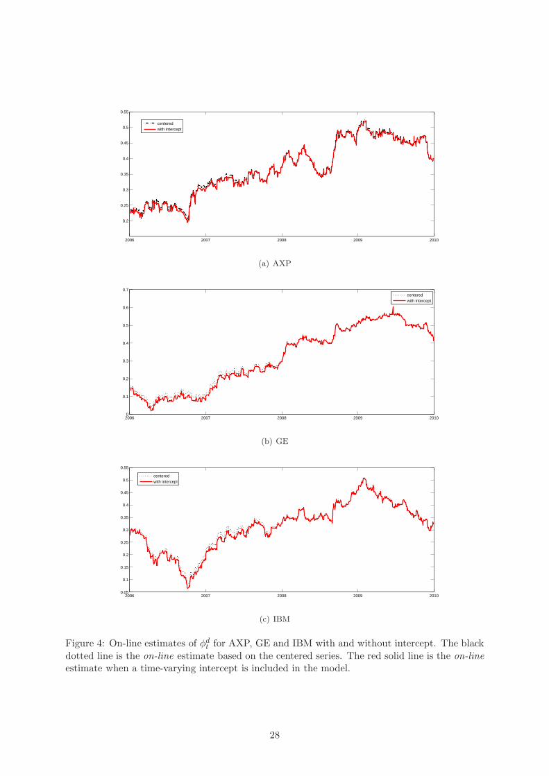
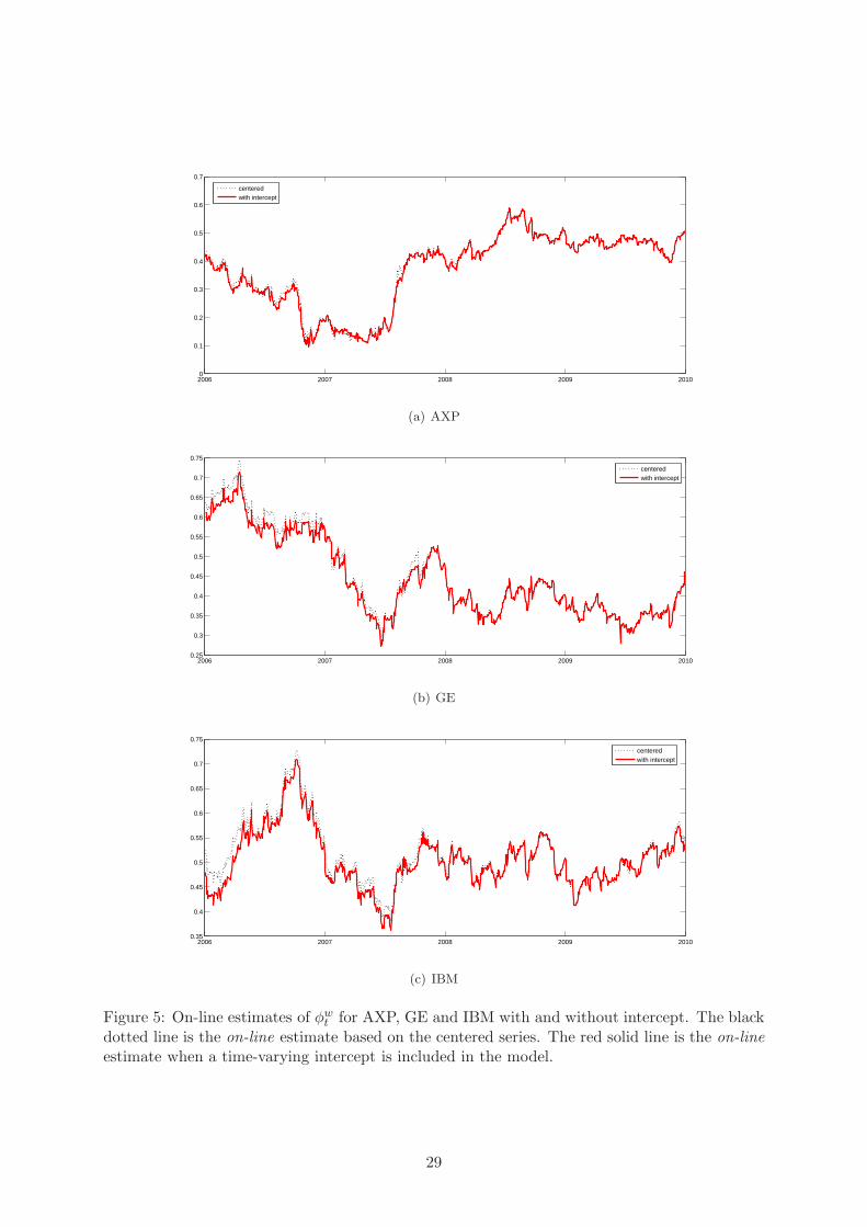
An explanation for this result emerges from Figures 4, 5 and 6, the estimates of φdt , φ

wt and φm

t

are almost identical to those obtained on the centered series, since the variation of µt = αt/(1−

φdt − φw

t − φmt ) is generally negligible when compared to the variation of the HAR parameters.

The only difference is in the estimates of φmt , in Figure 6, which is probably the consequence of

9

the lack of identification of µt during the year 2007, see Figure 7. In particular, from Figure 7

emerges that, when the largest eigenvalue of the TV-HAR characteristic polynomial is above 1,

the estimated unconditional mean, µt, is no longer identified.

The impulse response functions (IRF) calculated with two different sets of parameters, ob-

tained at different points in time, are plotted in Figure 8. There is an increase in volatility

persistence during the crisis. For example, the impact of an innovation on the one-step-ahead

volatility is approximately 30% larger during the financial crisis than during previous periods.

After one month, the gap between the two IRFs remains above 10%. This suggests that the

increasing role of the daily volatility component during the financial crisis is reflected in an

increase in the persistence of the volatility process.

Figures 9 - 13 present the results for the sequential indirect inference estimation of the TFSV

model. Consistently with the assumption that the changes in persistence are only due to changes

in the autoregressive structure of the HAR, the parameter ω, for both γ2(t) and ζ2(t), is kept

fixed and equal to half the sample average of RV . With regard to the fitting of the TFSV

model, Figure 9 plots the estimated objective function value, Ξt, for the period January 2006 -

December 2009. There is a notable difference between the dynamic behavior of the Ξt for the

stocks belonging to the financial sector and the others. In particular, on average Ξt is higher

for the banking sector, and it increases sharply during the period of the financial crisis. This

indicates that the TFSV model may be not flexible enough to capture the extent of variation

in the volatility dynamics of the financial stocks during the crisis. On the other hand, for the

other companies, Ξt remains more stable throughout the whole sample, with the exception of

GE, which experienced serious financial distress during the period January 2008 - March 2009.

The structural parameters governing the speeds of mean reversion display an interesting

dynamic pattern. The parameter κ, the speed of mean reversion of the fast moving factor,

ranges between 5 and 60 as shown in Figure 10. In particular, the parameter κ is smaller, on

average, for the banking sector than for the other stocks. This means that the volatility factor,

γ2(t), for the banking sector, reverts slower than the other stocks and hence is more persistent.

On the other hand, there is no a dominant trending pattern in the dynamic behavior of κ for

the other stocks. The parameter δ, see Figure 11, governs the speed of mean reversion of the

persistent factor. In all cases the estimates are close to 0, meaning that ζ2(t) is a close-to-unit-

root process, thus introducing high persistence in the volatility series. On average, the estimated

parameters are close to those found by Corsi and Reno (2012), based on the full sample. However,

10

Figures 10 and 11 show the extent of the time variation of the structural parameters when they

are sequentially estimated. This is particularly true for the parameters governing the volatility

of the volatility, in Figures 12 and 13. The parameter ν, which represents the volatility of

the persistent factor, has an upward trend, while η does not have a clear trend pattern and it

varies around 0.05. On the other hand, ν increases from 0.01 to 0.03 for the banking sector

and from 0.005 to 0.015 for the other stocks. This means that during the financial crisis, the

relative weight of the persistent volatility component increases with respect to the noisy factor,

especially for the banking sector, so that the volatility becomes more persistent and more volatile

at the same time. The increase of the volatility of the persistent factor during the financial crisis

not only induces the observed growth of the volatility levels, but also increases the degree of

uncertainty around its long-run level. Therefore, the persistent volatility component, which

mainly affects the size of the return variance and the investor’s consumption in the long-run,

plays an important role in the pricing of options and becomes more and more relevant as the the

crisis approaches. Hence, the variations in the parameter ν, which summarizes the uncertainty of

the investors toward the long-run investments, are responsible not only for the observed changes

in persistence but also for the increase of the volatility of volatility.

4.1 Time-varying volatility smile

A possible application to evaluate the consequences of the extent of time variation of the SV

parameters is in option pricing. The consequence of the variation in the SV parameters are

analyzed focusing at the evolution of the volatility smile curve, as the parameters of the TFSV

model are updated. For each day t, we extend the algorithm of Andersson (2003) in order to

compute the time-varying implied volatility smile:

i. At time t, a new option contract (a call) is issued with fixed time-to-maturity (90 days),

with underlying price S0.

ii. Trajectories from the TFSV model (4), are simulated with the parameter set Ψ̂t. The

simulated returns and volatility paths cover the 90 days horizon with 10 intradaily obser-

vations, for a total of 900 steps.

iii. The average annualized volatility is calculated for each path generated and the call price,

CBS , is computed according to the Black and Scholes (1973) formula with a grid of l

possible values of the strike price K = [K1,K2, . . . ,Kl−1,Kl].

11

iv. Replicate S̄ = 100 times points i) - iii).

v. Find the annualized implied volatility, V , for each value of K, such that it minimizes

the distance between the average of the S̄ generated call prices, CBS , and the Black and

Scholes (1973) prices computed with constant volatility.

vi. Iterate points i) - v) for each value of t = 1, . . . , T ;

vii. Obtain a matrix of values of V for each day t and for each strike price K.

The outcome of the procedure outlined above is presented in Figure 14, which shows the

evolution of the implied volatility smile, based on the volatility parameters of BAC. The

underlying price, S0, is assumed to be always equal to 50, while K1 = 37 and Kl = 63. The

level of the implied volatility increases, as expected when the return and volatility trajectories

are generated according to the parameters estimated during the period of the crisis. This is due

to the increase in the persistence of the volatility series such that there is a higher probability

of observing volatility values far from the long-run mean. Interestingly, this behavior is mainly

generated by an increase in the volatility of the persistent factor and not by a structural break in

the long-run mean of the process. Moreover, we observe a higher curvature of the smile during

the financial crisis, as measured by the ratio

ξ(t1, t2) =(V t2

K1+ V t2

Kl)/2− V t2

S0

(V t1K1

+ V t1Kl)/2− V t1

S0

× 100 − 100, (8)

where VK1, VKl

and VS0are annualized implied volatilities corresponding to K1, Kl and S0,

while t1 and t2 indicate two different periods of time in which V is computed. Similarly to the

previous analysis, choosing t1 equal to December 31, 2007 and t2 equal to December 31, 2008

leads to a value of ξ equal to 47%. This means that the curvature of the volatility smile has

increased about 47% as a consequence of the changes in the SV parameters during the financial

crisis. In contrast to the findings in Pena et al. (1999), it seems that high volatility periods,

characterized by higher persistence and higher volatility of volatility, tend to be associated

with a larger curvature of the smile. Carr and Wu (2007) relates the curvature of the smile,

measured with the butterfly spread, to fat-tails or positive excess kurtosis in the risk neutral

return distribution. We find empirical support for this evidence and we relate it to the increase

of the volatility of volatility during the financial crisis. In particular, we show that a Heston-

type SV model with time varying parameters is able to generate the stochastic variation of the

12

implied volatility smile observed by Carr and Wu (2007). This findings are coherent with the

generalization of the SV models proposed by Barndorff-Nielsen and Veraart (2013), who suggest

a stochastic model for the volatility of volatility relating it to the possibility of explaining the

variance risk premium as document Carr and Wu (2009).

5 Monte Carlo Simulations

The results of the simulations presented in this section are intended to verify that the empirical

results outlined in Section 4 are not spuriously induced by the adopted estimation method. In

particular, the estimation procedure outlined in Appendix A does not allow to test whether

the variation of the parameters is statistically significant. Therefore this set of Monte Carlo

simulations evaluates the ability of the on-line method to correctly estimate the time variation in

the parameters and to show the robustness of the selection method for the forgetting parameter,

λ.

Firstly, we verify whether the on-line method does not induce spurious variation in the TV-

HAR estimates. Therefore, the first set of Monte Carlo simulations is carried out according to

the following setup. We simulate S = 1000 times series of T = 1200 observations from a HAR

model with constant parameters, φd = 0.4, φw = 0.4 and φm = 0.15. The variance of εt is

assumed to follow a GARCH(1,1)

σ2ε,t = ω + αǫ2t−1 + βσ2

ε,t−1, (9)

with ω = 0.01, α = 0.05 and β = 0.90. For each Monte Carlo replication, the TV-HAR

is estimated with a different choice of λ, where the latter is defined on the grid of values

[0.95, 0.955, . . . , 0.995, 1]. Minimizing the mean squared one-step-ahead prediction error, the

value of λ is found to be equal to 1 in 89% of cases. When λ = 1, the variability of the pa-

rameters is almost zero and the estimates are centered on the true values. Figure 15 shows the

estimated TV-HAR parameters when the DGP is the constant HAR. The estimated parameters

are extremely smooth and display small variation around the constant parameters. This means

that when the parameters are constant, the on-line estimation method does not induce spurious

variability, but the extent of time-variation in the estimates is negligible.

Secondly, we verify whether the parameter estimates obtained with the on-line method follow

the true variation of the TV-HAR parameters. Therefore, in the second Monte Carlo setup, we

13

simulate S = 1000 times a series of T = 1200 observations from model (3) where, in each

Monte Carlo replication, the TV-HAR parameters are those estimated on the log-RV series of

AXP , see Section 4. The only sources of randomness are therefore the TV-HAR innovations, εt,

which, as before, are assumed to be Gaussian with conditional variance evolving as in equation

(9). In 76.5% of the cases, the value of λ is chosen to be equal to 0.995, while in 18% of

cases it is chosen to be equal to 0.99%. Figure 16 reports the data-generating parameters with

the 90% confidence intervals obtained from the Monte Carlo estimates. The 90% confidence

intervals contain the data-generating values in all cases, suggesting that the methodology is able

to capture the variation in the parameters. It should be noted that, due to the recursive nature

of the estimation algorithm, the confidence intervals are particularly wide at the beginning of

the sample, while they narrow as the information set becomes larger. We can conclude that, the

on-line approach yields reliable estimates of the TV-HAR parameters and the proposed method

for the choice of λ provides a robust selection method for the updating mechanism of the new

information.

Thirdly, we verify whether the observed variation in the TV-HAR cannot be generated by

a structural model with constant parameters. In particular, our goal is to evaluate whether

the variation in the TV-HAR estimates is not spuriously induced by the on-line estimation

algorithm, while the parameters of the TFSV model are constant. We therefore simulate S =

1000 daily RV series from model (4), holding the structural parameters constant. Consistently

with the findings presented in Section 4, the structural parameters are: κ = 5, δ = 0.001,

η = 0.05 and ν = 0.01. In particular, each RV series is generated with M̄ = 78 intradaily

returns for T = 1500 days. Figure 17 reports the estimation results. The on-line estimates are

generally close to the OLS estimates, which are based on the full sample, and they always lie

inside the OLS 90% confidence bands. This confirms that the observed variation in the TV-HAR

estimates is not induced by the adopted on-line estimation method, but it reflects the presence

of changes in the structural parameters.

Finally, we evaluate whether an increase in the volatility of the persistent volatility factor in

the TFSV induces the TV-HAR parameters to follow the trajectories obtained with the on-line

estimation method. Therefore, in the final Monte Carlo simulations, we let the parameter ν

in the TFSV model to be time-varying, with a dynamic behavior as in Figure 13. The other

structural parameters are kept constant at the values κ = 5, δ = 0.001, η = 0.05. Figure

18 shows strong variation in the TV-HAR parameters, which is consistent with the findings

14

presented in the empirical analysis. In particular, the weight of the daily volatility component

sharply increases, while the weekly and monthly volatility terms become less and less relevant

at the end of the sample. Compared to the OLS estimates, based on the full sample, the

TV-HAR parameters have clear trends, similar to those obtained with the observed realized

volatility series, and they generally lie outside the 90% confidence bands. These results confirm

the reliability of the inference methods adopted and the robustness of the empirical analysis.

6 Conclusions

The persistent nature of equity volatility as a mixture of processes at different frequencies is

investigated by means of a TFSV model. The parameters are estimated using a novel and fast

algorithm based on the state-space representation of the TV-HAR, as auxiliary model in the

sequential indirect inference estimation. From the TV-HAR estimates it emerges an increasing

role of the daily volatility component during the financial crisis, whereas the monthly term

becomes insignificant. The main finding that arise from the estimates of the TFSV model is the

crucial role played by the volatility of the persistent volatility factor during the financial crisis.

This induces the RV dynamics to diverge from the long run mean and to become more and more

volatile. From a financial point of view, this evidence can be interpreted as an increase of the

uncertainty about the long-run asset values, thus generating excess kurtosis. As a consequence,

the implied volatility curve changes its shape and curvature along with the updating of the SV

parameters and the increase of the volatility of volatility.

References

Andersen, T. and Bollerslev, T. (1998). Answering the skeptics: Yes, standard volatility models

do provide accurate forecasts. International Economic Review, 39:885–905.

Andersen, T. G., Bollerslev, T., and Diebold, F. X. (2007). Roughing it up: Including jump

components in the measurement, modeling, and forecasting of return volatility. The Review

of Economics and Statistics, 89:701–720.

Andersen, T. G., Bollerslev, T., Diebold, F. X., and Labys, P. (2001). The distribution of

exchange rate volatility. Journal of the American Statistical Association, 96:42–55.

15

Andersen, T. G., Bollerslev, T., Diebold, F. X., and Labys, P. (2003). Modeling and forecasting

realized volatility. Econometrica, 71:579–625.

Andersen, T. G., Bollerslev, T., and Huang, X. (2011). A reduced form framework for modeling

volatility of speculative prices based on realized variation measures. Journal of Econometrics,

160:176–189.

Andersson, K. (2003). Stochastic volatility. Technical report, U.U.D.M. Project Report, De-

partment of Mathematics, Uppsala University.

Asai, M., McAleer, M., and Medeiros, M. C. (2012). Modelling and forecasting noisy realized

volatility. Computational Statistics & Data Analysis, 56:217–230.

Barndorff-Nielsen, O. E. and Shephard, N. (2002). Estimating quadratic variation using realized

variance. Journal of Applied Econometrics, 17(5):457–477.

Barndorff-Nielsen, O. E. and Veraart, A. E. D. (2013). Stochastic volatility of volatility and

variance risk premia. Journal of Financial Econometrics, 11:1–46.

Bauwens, L. and Storti, G. (2009). A component GARCH model with time varying weights.

Studies in Nonlinear Dynamics & Econometrics, 13:1–24.

Black, F. and Scholes, M. (1973). The pricing of options and corporate liabilities. Journal of

Political Economy, 81:637654.

Bollerslev, T. (1986). Generalized autoregressive conditional heteroskedasticity. Journal of

Econometrics, 31:307–327.

Bollerslev, T. and Zhou, H. (2002). Estimating stochastic volatility diffusion using conditional

moments of integrated volatility. Journal of Econometrics, 109:33–65.

Bordignon, S. and Raggi, D. (2012). Long memory and nonlinearities in realized volatility: a

markov switching approach. Computational Statistics and Data Analysis, 56:3730–3742.

Carr, P. and Wu, L. (2007). Stochastic skew for currency options. Journal of Financial Eco-

nomics, 89:213–247.

Carr, P. and Wu, L. (2009). Variance risk premiums. Review of Financial Studies, 22:1311–1341.

16

Choi, K., Yu, W. C., and Zivot, E. (2010). Long memory versus structural breaks in modeling

and forecasting realized volatility. Journal of International Money and Finance, 29:857–875.

Cogley, T. and Sargent, T. (2005). Drifts and volatilities: Monetary policies and outcomes in

the post wwii u.s. Review of Economic Dynamics, 8:262–302.

Corsi, F. (2009). A simple approximate long-memory model of realized volatility. Journal of

Financial Econometrics, 7:174–196.

Corsi, F., Mittnik, S., Pigorsch, C., and Pigorsch, U. (2008). The volatility of realized volatility.

Econometric Reviews, pages 46–78.

Corsi, F. and Reno, R. (2012). Discrete-time volatility forecasting with persistent leverage effect

and the link with continuous-time volatility modeling. Technical report, Journal of Business

and Economic Statistics forthcoming.

Covitz, D. M., N., L., and Suarez, G. A. (2012). The evolution of a financial crisis: Collapse of

the asset-backed commercial paper market. Journal of Finance, Forthcoming.

Dahlhaus, R. and Rao, S. S. (2007a). A recursive online algorithm for the estimation of time-

varying arch parameters. Bernoulli, 13:389–422.

Dahlhaus, R. and Rao, S. S. (2007b). Statistical inference for time-varying arch processes.

Annals of Statistics, 34:1075–1114.

Durbin, J. and Koopman, S. (2001). Time Series Analysis by State Space Methods. Oxford

University Press, Oxford, UK.

Eklund, J. and Karlsson, S. (2007). Forecast combination and model averaging using predictive

measures. Econometric Reviews, 26(2-4):329–363.

Engle, R. F. (1982). Autoregressive conditional heteroscedasticity with estimates of the variance

of united kingdom inflation. Econometrica, 50:987–1008.

Engle, R. F. and Rangel, J. G. (2008). The spline-garch model for low-frequency volatility and

its global macroeconomic causes. Review of Financial Studies, 21:1187–1222.

Fagin, S. (1964). Recursive linear regression theory, optimalter theory, and error analyses of

optimal systems. IEEE International Convention Record Part, pages 216 – 240.

17

Forsberg, L. and Ghysels, E. (2007). Why do absolute returns predict volatility so well? Journal

of Financial Econometrics, 5-1:31–67.

Frijns, B., Lehnert, T., and Zwinkels, R. C. (2011). Modeling structural changes in the volatility

process. Journal of Empirical Finance, 18:522–532.

Gallant, A. R., Hsu, C.-T., and Tauchen, G. (1999). Using daily range data to calibrate volatil-

ity diffusions and extract the forward integrated variance. The Review of Economics and

Statistics, 81:617–631.

Gerlach, G., Carter, C., and Kohn, R. (2000). Bayesian inference for dynamic mixture models.

Journal of the American Statistical Association, 95:819 – 828.

Geweke, J. (2005). Contemporary Bayesian Econometrics and Statistics. Wiley, New York,

USA.

Ghysels, E., Santa-Clara, P., and Valkanov, R. (2006). Predicting volatility: getting the most

out of return data sampled at different frequencies. Journal of Econometrics, 131:59–95.

Giot, P. and Laurent, S. (2004). Modelling daily value-at-risk using realized volatility and arch

type models. Journal of Empirical Finance, 11:379–398.

Gourieroux, C., Monfort, A., and E., R. (1993). Indirect inference. Journal of Applied Econo-

metrics, 8:85–113.

Groen, J., Paap, R., and Ravazzolo, F. (2012). Real-time inflation forecasting in a changing

world. Journal of Business and Economic Statistics, 31:28–44.

Jazwinsky, A. (1970). Stochastic Processes and Filtering Theory. New York: Academic Press.

Koop, G. and Korobilis, D. (2012). Forecasting inflation using dynamic model averaging. In-

ternational Economic Review, 53:867–886.

Koop, G., Leon-Gonzalez, R., and Strachan, R. (2009). On the evolution of the monetary policy

transmission mechanism. Journal of Economic Dynamics and Control, 33:997 – 1017.

Lieberman, O. and Phillips, P. C. B. (2008). Refined inference on long-memory in realized

volatility. Econometric Reviews, 27:254–267.

18

Liu, C. and Maheu, J. M. (2008). Are there structural breaks in realized volatility? Journal of

Financial Econometrics, 1:1–35.

Maheu, J. M. and McCurdy, T. H. (2002). Nonlinear features of realized fx volatility. The

Review of Economics and Statistics, 84:668–681.

Martens, M., Van Dijk, D., and de Pooter, M. (2009). Forecasting s&p 500 volatility: Long

memory, level shifts, leverage effects, day-of-the-week seasonality, and macroeconomic an-

nouncements. International Journal of Forecasting, 25:282–303.

McAleer, M. and Medeiros, M. C. (2008). A multiple regime somooth transition heterogeneous

autoregressive model for long memory and asymmetries. Journal of Econometrics, 147:104–

119.

McAleer, M. and Medeiros, M. C. (2011). Forecasting realized volatility with linear and nonlinear

models. Journal of Economic Surveys., 25:6–18.

Meddahi, N. (2002). A theoretical comparison between integrated and realized volatility. Journal

of Applied Econometrics, 17:479–508.

Meddahi, N. (2003). Arma representation of integrated and realized variances. Econometrics

Journal, 6:335–356.

Pena, I., Rubio, G., and Serna, G. (1999). Why do we smile? On the determinants of the implied

volatility function. Journal of Banking & Finance, 23:1151–1179.

Primiceri, G. (2005). Time varying structural vector autoregressions and monetary policy. Re-

view of Economic Studies, 72:821 – 852.

Raftery, A., Karny, M., and Ettler, P. (2010). Online prediction under model uncertainty via

dynamic model averaging: Application to a cold rolling mill. Technometrics, 52:52–66.

19

A Estimation Method

The estimation methodology requires a state-space specification of the TV-HAR model in equa-

tion (3),

yt = Ztθt + εt εt ∼ N(0,Ht),

θt = θt−1 + ηt ηt ∼ N(0,Qt),

(10)

where yt is the observed variable, Zt = [ydt−1, ywt−1, y

mt−1] is a 1 × 3 vector containing the HAR

lag structure, and θt = [φdt , φ

wt , φ

mt ]′ is a 3 × 1 vector of time varying parameters, which are

assumed to follow random-walk dynamics. In this setup, the HAR parameters are considered as

state variables, while the past values of yt are the explanatory variables. The errors εt and ηt

are assumed to be mutually independent at all leads and lags.

Once model (3) is casted in the state space form (10) , the parameter vector θt can be easily

estimated with a standard Kalman filtering technique. The prediction step for given values of

Ht and Qt is:

θt|t−1 = θt−1|t−1

Σt|t−1 = Σt−1|t−1 +Qt

ǫt|t−1 = yt − Ztθt|t−1.

(11)

However, the estimation of Qt requires computationally intensive algorithms, such as MCMC

methods. Therefore Raftery et al. (2010) suggest to substitute the prediction equation of Σt|t−1

in equation (11) with

Σt|t−1 =1

λΣt−1|t−1, (12)

so that Qt = (λ−1 − 1)Σt−1|t−1 where 0 < λ < 1. This approach has been introduced in

the state space literature by Fagin (1964) and Jazwinsky (1970), to reduce the computational

burden of the traditional Kalman filter. Raftery et al. (2010) provide a detailed discussion of this

approximation, especially regarding the tuning parameter λ. The parameter λ can be considered

as a forgetting factor, since the specification in equation (12) implies that the weight associated

to the observations j periods in the past is equal to λj . Following Raftery et al. (2010) and

Koop and Korobilis (2012), the parameter λ must be chosen large enough in order to guarantee

20

a sufficient degree of smoothness. For quarterly data, Koop and Korobilis (2012) suggest that λ

should be chosen between 0.95 and 0.99. In this paper, the choice of λ is such that it minimizes

the mean squared one-step-ahead prediction error. With daily data, we find that the optimal

λ is equal to 0.995. This value for λ is consistent with a fairly stable model where changes of

the coefficients are gradual. For example, observations 22 days ago receive approximately 90%

of the weight given to the last observation, whereas with λ = 0.95 they receive approximately

33%.

It is interesting to note that the simplification used by Raftery et al. (2010) implies that Qt

does not need to be estimated. However, a method to estimate Ht, which is the variance of the

irregular component, is still required. Raftery et al. (2010) recommend a simple plug-in method

where an estimate of Ht is given by

Ht|t−1 =1

t

t∑

j=1

[

(yj + Zjθj−1|j−1)2 − ZjΣj|j−1Z

′

j

]

. (13)

Since RV is shown to be heteroskedastic, see Corsi et al. (2008), so that the error variance is likely

to change over time, we adopt an alternative method to compute the variance Ht. Following

Koop and Korobilis (2012), Ht follows an exponentially weighted moving average,

Ht|t−1 = κHt−1|t−1 + (1− κ)(yt − Ztθt|t−1)2, (14)

with κ = 0.94, so that the variance of the error term is allowed to vary over time and the

estimates of the TV-HAR parameters are robust to heteroskedastic effects, especially during the

financial crisis.

Finally, equations (15) and (16), conditional on Ht|t−1, are all analytical expressions and thus

no simulation-based methods are required. In particular, given Ht|t−1 and Σt|t−1, the updating

recursions for the parameters of the model are given by:

θt|t = θt|t−1 +Σt|t−1Zt(Ht|t−1 + ZtΣt|t−1Z′

t)−1(yt − Ztθt|t−1) (15)

and

Σt|t = Σt|t−1 −Σt|t−1Zt(Ht|t−1 + ZtΣt|t−1Z′

t)−1ZtΣt|t−1. (16)

Clearly different estimation approaches, based on Bayesian and maximum likelihood meth-

21

ods, can be applied. In principle, maximum likelihood estimation with the Kalman filter routine

could be an alternative, see Durbin and Koopman (2001) for an introduction. However, the

on-line method avoids the empirical drawbacks of standard likelihood methods such as multiple

maxima, instability and lack of identification of the state vector parameters. Alternatively, in

the Bayesian framework, an interesting approach has been proposed by Groen et al. (2012), who

suggest to draw posteriors using an extension of the mixture sampling of Gerlach et al. (2000).

This approach, although reliable, is computationally intensive and requires a proper choice of

the priors. On the other hand the on-line estimation method allows for a fast updating of the

parameters and does not require to select optimal priors for the initial states. The sequential

method is also particularly appealing for real-time financial decisions, where the trader needs to

update the parameters as new observations arrive. Indeed, the updating of the parameters only

requires to run equations (12), (14), (15) and (16) once a new observation is available. This

explains why this class of methods is often called on-line.

22

B Figures and Tables

MIN DATE MAX DATE RANGE

φd

AXP 0.2032 2006-10-06 0.5257 2009-02-06 0.3225

BA 0.1803 2006-10-24 0.5349 2009-02-04 0.3546

BAC 0.2784 2006-04-12 0.6157 2008-09-16 0.3373

C 0.2372 2006-08-08 0.6167 2009-05-13 0.3795

GE 0.0390 2006-04-13 0.6064 2009-06-18 0.5674

GS 0.2681 2006-04-07 0.6321 2009-01-29 0.3640

IBM 0.0819 2006-10-05 0.5109 2009-01-29 0.4290

JPM 0.2409 2006-04-12 0.6948 2009-01-27 0.4539

MCD 0.1139 2006-10-03 0.4275 2009-02-12 0.3136

MET 0.1804 2006-02-24 0.5533 2009-02-20 0.3729

MS 0.2275 2006-12-26 0.6344 2009-01-27 0.4070

PG 0.1071 2006-03-24 0.4004 2009-02-09 0.2933

T 0.0261 2006-04-13 0.4263 2008-12-02 0.4002

WFC 0.0971 2006-04-17 0.5727 2009-01-26 0.4756

XOM 0.2299 2006-10-11 0.5840 2009-01-15 0.3541

φw

AXP 0.1086 2007-05-14 0.5927 2008-07-15 0.4841

BA 0.2353 2009-10-16 0.5649 2006-02-21 0.3297

BAC 0.1002 2007-07-17 0.5047 2006-04-12 0.4045

C 0.2150 2007-07-13 0.5233 2008-08-28 0.3083

GE 0.2768 2009-06-18 0.7438 2006-04-18 0.4669

GS 0.2171 2007-03-21 0.5208 2007-12-10 0.3037

IBM 0.3802 2007-07-23 0.7263 2006-10-05 0.3461

JPM 0.1949 2007-06-26 0.5517 2008-07-15 0.3568

MCD 0.2284 2006-05-10 0.5595 2008-12-30 0.3312

MET 0.2476 2007-03-20 0.6042 2007-12-10 0.3565

MS 0.2544 2007-07-13 0.5187 2007-11-09 0.2643

PG 0.2533 2007-03-20 0.6889 2006-03-24 0.4356

T 0.3437 2007-03-15 0.7239 2006-02-21 0.3802

WFC 0.1045 2007-04-30 0.5725 2008-09-18 0.4680

XOM 0.3220 2009-11-13 0.6519 2006-10-11 0.3299

φm

AXP -0.0233 2008-09-19 0.5877 2006-11-10 0.6110

BA 0.0201 2008-07-22 0.3670 2007-03-19 0.3469

BAC -0.0062 2008-09-18 0.4213 2007-08-14 0.4275

C -0.0099 2008-08-21 0.4054 2006-08-11 0.4153

GE 0.0298 2009-06-18 0.7438 2006-04-18 0.4669

GS -0.0042 2008-09-18 0.3993 2006-05-11 0.4034

IBM -0.0158 2008-12-31 0.2358 2007-01-26 0.2516

JPM -0.0356 2008-09-19 0.3749 2007-06-21 0.4105

MCD 0.0104 2008-12-30 0.5100 2007-01-26 0.4996

MET -0.0125 2008-09-19 0.4783 2007-06-04 0.4908

MS -0.0091 2008-09-18 0.3781 2007-02-22 0.3872

PG -0.0027 2008-07-28 0.3116 2007-07-16 0.3143

T 0.0133 2008-12-16 0.3321 2007-01-23 0.3188

WFC -0.0108 2008-09-18 0.5363 2007-02-22 0.5471

XOM -0.0460 2007-12-10 0.1068 2007-07-11 0.1528

Table 1: Summary statistics of the TV-HAR parameters. Table reports the minimum and themaximum of the observed values of the TV-HAR parameters with the corresponding dates. Lastcolumn reports the range of variation of the parameters, calculated as MAX −MIN .

23

RMSEr RMSEu log(PL)r log(PL)u

AXP 0.4763 0.4786 -421.9994 -424.9833BA 0.5073 0.5070 -468.7136 -466.9602

BAC 0.5469 0.5506 -513.9557 -516.8078C 0.6154 0.6176 -578.2686 -580.6340GE 0.5578 0.5613 -525.0722 -526.7052GS 0.4835 0.4850 -399.1553 -399.1658IBM 0.4672 0.4705 -394.3845 -394.5168JPM 0.4545 0.4583 -390.1873 -394.0390MCD 0.5139 0.5146 -452.3584 -451.1535

MET 0.4948 0.4961 -450.8025 -451.1418MS 0.5131 0.5150 -426.0185 -427.4654PG 0.4987 0.5006 -424.8467 -422.7409

T 0.5157 0.5161 -458.1966 -456.0033

WFC 0.4888 0.4912 -430.6668 -433.5275XOM 0.4394 0.4407 -345.3549 -344.0124

Table 2: Out-of-sample forecast comparison. Table reports the RMSE and the log predictivelikelihood (log(PL)) for the model with (u) and without (r) the intercept. The out of sampleperiod starts from August 1, 2007 to December 31, 2009.

24

2006 2007 2008 2009 20100.2

0.25

0.3

0.35

0.4

0.45

0.5

0.55

(a) φdt of AXP

2006 2007 2008 2009 20100

0.1

0.2

0.3

0.4

0.5

0.6

0.7

(b) φdt of GE

2006 2007 2008 2009 20100.05

0.1

0.15

0.2

0.25

0.3

0.35

0.4

0.45

0.5

0.55

(c) φdt of IBM

Figure 1: On-line estimates of φdt for AXP, GE and IBM. The solid black line is the on-line

estimate, while the blue dotted line is the OLS estimate based on the full sample. The dashedred lines correspond to the 90% confidence band.

25

2006 2007 2008 2009 20100.1

0.15

0.2

0.25

0.3

0.35

0.4

0.45

0.5

0.55

0.6

(a) φwt of AXP

2006 2007 2008 2009 20100.25

0.3

0.35

0.4

0.45

0.5

0.55

0.6

0.65

0.7

0.75

(b) φwt of GE

2006 2007 2008 2009 20100.35

0.4

0.45

0.5

0.55

0.6

0.65

0.7

0.75

(c) φwt of IBM

Figure 2: On-line estimates of φwt for AXP, GE and IBM. The solid black line is the on-line


26

2006 2007 2008 2009 2010−0.1

0

0.1

0.2

0.3

0.4

0.5

0.6

(a) φmt of AXP

0 100 200 300 400 500 600 700 800 900 10000

0.05

0.1

0.15

0.2

0.25

0.3

0.35

0.4

0.45

(b) φmt of GE

2006 2007 2008 2009 2010−0.05

0

0.05

0.1

0.15

0.2

0.25

0.3

(c) φmt of IBM

Figure 3: On-line estimates of φmt for AXP, GE and IBM. The solid black line is the on-line


27

2006 2007 2008 2009 2010

0.2

0.25

0.3

0.35

0.4

0.45

0.5

0.55

centeredwith intercept

(a) AXP

2006 2007 2008 2009 20100

0.1

0.2

0.3

0.4

0.5

0.6

0.7


(b) GE

2006 2007 2008 2009 20100.05

0.1

0.15

0.2

0.25

0.3

0.35

0.4

0.45

0.5

0.55


(c) IBM

Figure 4: On-line estimates of φdt for AXP, GE and IBM with and without intercept. The black

dotted line is the on-line estimate based on the centered series. The red solid line is the on-line

estimate when a time-varying intercept is included in the model.

28

2006 2007 2008 2009 20100

0.1

0.2

0.3

0.4

0.5

0.6

0.7


(a) AXP

2006 2007 2008 2009 20100.25

0.3

0.35

0.4

0.45

0.5

0.55

0.6

0.65

0.7

0.75


(b) GE

2006 2007 2008 2009 20100.35

0.4

0.45

0.5

0.55

0.6

0.65

0.7

0.75


(c) IBM

Figure 5: On-line estimates of φwt for AXP, GE and IBM with and without intercept. The black



29

2006 2007 2008 2009 2010−0.1

0

0.1

0.2

0.3

0.4

0.5

0.6


(a) AXP

2006 2007 2008 2009 2010−0.05

0

0.05

0.1

0.15

0.2

0.25

0.3

0.35

0.4

0.45


(b) GE

2006 2007 2008 2009 2010−0.1

−0.05

0

0.05

0.1

0.15

0.2

0.25


(c) IBM

Figure 6: On-line estimates of φmt for AXP, GE and IBM with and without intercept. The black



30

2006 2007 2008 2009 2010−800

−700

−600

−500

−400

−300

−200

−100

0

100

200

(a) AXP

2006 2007 2008 2009 2010−20

−15

−10

−5

0

5

10

(b) GE

2006 2007 2008 2009 2010−20

−15

−10

−5

0

5

10

(c) IBM

Figure 7: On-line estimates of µt = αt/(1− φdt − φw

t − φmt ) for AXP, GE and IBM.

31

0 2 4 6 8 10 12 14 16 18 20 220

0.2

0.4

0.6

0.8

1

Period

Res

pons

e

Impulse Response

2009−02−06

2006−11−10

(a) AXP

0 2 4 6 8 10 12 14 16 18 20 220

0.2

0.4

0.6

0.8

1

Period

Res

pons

e

Impulse Response

2009−06−18

2006−04−18

(b) GE

0 2 4 6 8 10 12 14 16 18 20 220

0.2

0.4

0.6

0.8

1

Period

Res

pons

e

Impulse Response

2009−01−29

2007−01−26

(c) IBM

Figure 8: Impulse response functions based on two different sets of parameters. The dates, t1and t2, are chosen such that the difference |φd

t1− φd

t2| is maximized, see Table 1.

32

2006 2007 2008 2009 20100

1

2

3

4

5

6

7

8

9

10

χ

AXP

χBAC

χC

χGS

χJPM

χMET

χMS

χWFC

(a) Ξt: BANK SECTOR

2006 2007 2008 2009 20100

1

2

3

4

5

6

7

8

9

10

χBA

χGE

χIBM

χMCD

χPG

chiT

χXOM

(b) Ξt: OTHERS

Figure 9: Ξt criterion for the two-factors model. Panel (a) reports Ξt for the stocks belongingto the bank-financial sector, while Panel (b) reports the Ξt distance for the stocks belonging tothe other sectors of US economy.

33

2006 2007 2008 2009 20100

10

20

30

40

50

60

κ

AXP

κBAC

κC

κGS

κJPM

κMET

κMS

κWFC

(a) κ: BANK SECTOR

2006 2007 2008 2009 20100

10

20

30

40

50

60

κ

BA

κGE

κIBM

κMCD

κPG

κT

κXOM

(b) κ: OTHERS

Figure 10: Estimated parameter κ of the two-factors model. Panel (a) reports the parameter κfor the stocks belonging to the bank-financial sector, while Panel (b) reports the parameter κfor the stocks belonging to the other sectors of US economy.

34

2006 2007 2008 2009 20100

0.5

1

1.5

2

2.5

3

3.5x 10

−3

δ

AXP

δBAC

δC

δGS

δJPM

δMET

δMS

δWFC

(a) δ: BANK SECTOR

2006 2007 2008 2009 20100.4

0.6

0.8

1

1.2

1.4

1.6x 10

−3

δ

BA

δGE

δIBM

δMCD

δPG

δT

δXOM

(b) δ: OTHERS

Figure 11: Estimated parameter δ of the two-factors model. Panel (a) reports the parameter δfor the stocks belonging to the bank-financial sector, while Panel (b) reports the parameter δfor the stocks belonging to the other sectors of US economy.

35

2006 2007 2008 2009 20100.02

0.04

0.06

0.08

0.1

0.12

0.14

0.16

ηAXP

ηBAC

ηC

ηGS

ηJPM

ηMET

ηMS

ηWFC

(a) η: BANK SECTOR

2006 2007 2008 2009 20100

0.02

0.04

0.06

0.08

0.1

0.12

0.14

ηBA

ηGE

ηIBM

ηMCD

ηPG

ηT

ηXOM

(b) η: OTHERS

Figure 12: Estimated parameter η of the two-factors model. Panel (a) reports the parameter ηfor the stocks belonging to the bank-financial sector, while Panel (b) reports the parameter ηfor the stocks belonging to the other sectors of US economy.

36

2006 2007 2008 2009 20100

0.01

0.02

0.03

0.04

0.05

0.06

νAXP

νBAC

νC

νGS

νJPM

νMET

νMS

νWFC

(a) ν: BANK SECTOR

0 100 200 300 400 500 600 700 800 900 10000

0.005

0.01

0.015

0.02

0.025

0.03

νBA

νGE

νIBM

νMCD

νPG

νT

νXOM

(b) ν: OTHERS

Figure 13: Estimated parameter ν of the two-factors model. Panel (a) reports the parameter νfor the stocks belonging to the bank-financial sector, while Panel (b) reports the parameter νfor the stocks belonging to the other sectors of US economy.

37

2006

2007

2008

2009

37

42

47

52

57

620.45

0.5

0.55

0.6

Figure 14: Implied Volatility Smile Evolution based on the stochastic volatility parameters of BAC. The x-axis reports the dates, the y-axis reportsthe strike prices at maturity (90 days), which range from 40 to 60. The annualized volatility values are reported on the z-axis.

38

0 100 200 300 400 500 600 700 800 900 10000.2

0.25

0.3

0.35

0.4

0.45

0.5

0.55

estimated

true

(a) φd

0 100 200 300 400 500 600 700 800 900 10000.2

0.25

0.3

0.35

0.4

0.45

0.5

0.55

estimated

true

(b) φw

0 100 200 300 400 500 600 700 800 900 1000−0.1

−0.05

0

0.05

0.1

0.15

0.2

0.25

0.3

0.35

estimated

true

(c) φm

Figure 15: Estimates of the constant HAR parameters with the on-line method. Figures report the outcome of a single Monte Carlo estimate. Thedashed blue line is the true parameter, while the solid red line is the on-line estimate.

39

0 200 400 600 800 1000 1200−0.1

0

0.1

0.2

0.3

0.4

0.5

0.6

φd

90 % CI

90 % CI

(a) Online estimates of φdt with 90% Montecarlo confidence bands

0 200 400 600 800 1000 1200−0.2

−0.1

0

0.1

0.2

0.3

0.4

0.5

0.6

0.7

0.8

φw

90 % CI

90 % CI

(b) Online estimates of φwt with 90% Montecarlo confidence bands

0 200 400 600 800 1000 1200−0.2

0

0.2

0.4

0.6

0.8

1

1.2

φm

90% CI

90% CI

(c) Online estimates of φmt with 90% Montecarlo confidence bands

Figure 16: Estimates of the TV-HARV parameters with the on-line method. Figure report the true parameter (solid black line), and the 90%Monte Carlo confidence band (dashed red lines).

40

0 200 400 600 800 1000 1200

0.05

0.1

0.15

0.2

0.25

0.3

0.35

0.4

0.45

0.5

(a) φdt estimates

0 200 400 600 800 1000 12000.2

0.3

0.4

0.5

0.6

0.7

0.8

(b) φwt estimates

0 200 400 600 800 1000 1200−0.1

−0.05

0

0.05

0.1

0.15

0.2

0.25

0.3

0.35

0.4

(c) φmt estimates

Figure 17: On-line estimates of the TV-HAR parameters when the RV is generated from aTFSV model with constant parameters. The red solid line is the average for each t ∈ [1 : T ] ofthe on-line estimates. The dotted blue line is the average of the OLS estimates based on thefull sample, while the green dashed lines correspond to the 90% confidence bands of the OLSestimates.

41

0 200 400 600 800 1000 1200 14000.2

0.25

0.3

0.35

0.4

0.45

0.5

0.55

(a) φdt estimates

0 200 400 600 800 1000 1200 14000.15

0.2

0.25

0.3

0.35

0.4

0.45

0.5

0.55

0.6

0.65

(b) φwt estimates

0 200 400 600 800 1000 1200 1400−0.1

−0.05

0

0.05

0.1

0.15

0.2

0.25

0.3

0.35

(c) φmt estimates

Figure 18: On-line estimates of the TV-HAR parameters when the RV is generated from aTFSV model with time-varying parameters. The red solid line is the average for each t ∈ [1 : T ]of the on-line estimates. The dotted blue line is the average of the OLS estimates based on thefull sample, while the green dashed lines correspond to the 90% confidence bands of the OLSestimates.

42

Research Papers 2013

2012-45: Peter Reinhard Hansen and Allan Timmermann: Equivalence Between Out-of-Sample Forecast Comparisons and Wald

2012-46: Søren Johansen, Marco Riani and Anthony C. Atkinson: The Selection of ARIMA Models with or without Regressors

2012-47: Søren Johansen and Morten Ørregaard Nielsen: The role of initial values in nonstationary fractional time series models

2012-48: Peter Christoffersen, Vihang Errunza, Kris Jacobs and Hugues Langlois: Is the Potential for International Diversi…cation Disappearing? A Dynamic Copula Approach

2012-49: Peter Christoffersen, Christian Dorion , Kris Jacobs and Lotfi Karoui: Nonlinear Kalman Filtering in Affine Term Structure Models

2012-50: Peter Christoffersen, Kris Jacobs and Chayawat Ornthanalai: GARCH Option Valuation: Theory and Evidence

2012-51: Tim Bollerslev, Lai Xu and Hao Zhou: Stock Return and Cash Flow Predictability: The Role of Volatility Risk

2012-52: José Manuel Corcuera, Emil Hedevang, Mikko S. Pakkanen and Mark Podolskij: Asymptotic theory for Brownian semi-stationary processes with application to turbulence

2012-53: Rasmus Søndergaard Pedersen and Anders Rahbek: Multivariate Variance Targeting in the BEKK-GARCH Model

2012-54: Matthew T. Holt and Timo Teräsvirta: Global Hemispheric Temperature Trends and Co–Shifting: A Shifting Mean Vector Autoregressive Analysis

2012-55: Daniel J. Nordman, Helle Bunzel and Soumendra N. Lahiri: A Non-standard Empirical Likelihood for Time Series

2012-56: Robert F. Engle, Martin Klint Hansen and Asger Lunde: And Now, The Rest of the News: Volatility and Firm Specific News Arrival

2012-57: Jean Jacod and Mark Podolskij: A test for the rank of the volatility process: the random perturbation approach

2012-58: Tom Engsted and Thomas Q. Pedersen: Predicting returns and rent growth in the housing market using the rent-to-price ratio: Evidence from the OECD countries

2013-01: Mikko S. Pakkanen: Limit theorems for power variations of ambit fields driven by white noise

2013-02: Almut E. D. Veraart and Luitgard A. M. Veraart: Risk premia in energy markets

2013-03: Stefano Grassi and Paolo Santucci de Magistris: It’s all about volatility (of volatility): evidence from a two-factor stochastic volatility model

it’s all about volatility (of volatility): evidence from...

Documents