SANDIA REPORTSAND2009-0970Unlimited ReleasePrinted February 2009

IWA: an analysis program forisentropic wave measurements

Tommy Ao

Prepared bySandia National LaboratoriesAlbuquerque, New Mexico 87185 and Livermore, California 94550

Sandia is a multiprogram laboratory operated by Sandia Corporation,a Lockheed Martin Company, for the United States Department of Energy’sNational Nuclear Security Administration under Contract DE-AC04-94-AL85000.

Approved for public release; further dissemination unlimited.

Issued by Sandia National Laboratories, operated for the United States Department of Energyby Sandia Corporation.

NOTICE: This report was prepared as an account of work sponsored by an agency of the UnitedStates Government. Neither the United States Government, nor any agency thereof, nor anyof their employees, nor any of their contractors, subcontractors, or their employees, make anywarranty, express or implied, or assume any legal liability or responsibility for the accuracy,completeness, or usefulness of any information, apparatus, product, or process disclosed, or rep-resent that its use would not infringe privately owned rights. Reference herein to any specificcommercial product, process, or service by trade name, trademark, manufacturer, or otherwise,does not necessarily constitute or imply its endorsement, recommendation, or favoring by theUnited States Government, any agency thereof, or any of their contractors or subcontractors.The views and opinions expressed herein do not necessarily state or reflect those of the UnitedStates Government, any agency thereof, or any of their contractors.

Printed in the United States of America. This report has been reproduced directly from the bestavailable copy.

Available to DOE and DOE contractors fromU.S. Department of EnergyOffice of Scientific and Technical InformationP.O. Box 62Oak Ridge, TN 37831

Telephone: (865) 576-8401Facsimile: (865) 576-5728E-Mail: reports@adonis.osti.govOnline ordering: http://www.osti.gov/bridge

Available to the public fromU.S. Department of CommerceNational Technical Information Service5285 Port Royal RdSpringfield, VA 22161

Telephone: (800) 553-6847Facsimile: (703) 605-6900E-Mail: orders@ntis.fedworld.govOnline ordering: http://www.ntis.gov/help/ordermethods.asp?loc=7-4-0#online

2

SAND2009-0970Unlimited Release

Printed February 2009

IWA: an analysis program for isentropic wavemeasurements

Tommy AoDynamic Material Properties

Sandia National LaboratoriesP.O. Box 5800

Albuquerque, NM 87185

Abstract

IWA (Isentropic Wave Analysis) is a program for analyzing velocity profiles of isentropiccompression experiments. IWA applies incremental impedance matching correction to mea-sured velocity profiles to obtain in-situ particle velocity profiles for Lagrangian wave analysis.From the in-situ velocity profiles, material properties such as wave velocities, stress, strain,strain rate, and strength are calculated. The program can be run in any current version ofMATLAB (2008a or later) or as a Windows XP executable.

3

Acknowledgments

The IWA program is built upon the many discussion with Jim Asay. An earlier analysisprogram by Tracy Vogler provided the starting point for this work. Dan Dolan compiled theprogram into a Windows executable, and provided MATLAB support.

Experimental data used in the analysis example was made possible by the DICE facilitytechnicians who operate and maintain the Veloce pulsed power generator.

4

Contents

1 Introduction 9

1.1 Program summary . . . . . . . . . . . . . . . . . . . . . . . . . . . . . . . . . . . . . . . . . . . . . . . . 9

1.2 Overview of report . . . . . . . . . . . . . . . . . . . . . . . . . . . . . . . . . . . . . . . . . . . . . . . . 9

2 Theoretical background 11

2.1 Wave propagation . . . . . . . . . . . . . . . . . . . . . . . . . . . . . . . . . . . . . . . . . . . . . . . . . 11

2.2 Lagrangian wave analysis . . . . . . . . . . . . . . . . . . . . . . . . . . . . . . . . . . . . . . . . . . . 13

2.2.1 Material strength . . . . . . . . . . . . . . . . . . . . . . . . . . . . . . . . . . . . . . . . . . . 15

3 Program overview 19

3.1 Installing and running IWA . . . . . . . . . . . . . . . . . . . . . . . . . . . . . . . . . . . . . . . . . 19

3.1.1 MATLAB version . . . . . . . . . . . . . . . . . . . . . . . . . . . . . . . . . . . . . . . . . . . 19

3.1.2 Windows executable . . . . . . . . . . . . . . . . . . . . . . . . . . . . . . . . . . . . . . . . . 19

3.2 Graphical user interface . . . . . . . . . . . . . . . . . . . . . . . . . . . . . . . . . . . . . . . . . . . . 20

3.2.1 Main figure . . . . . . . . . . . . . . . . . . . . . . . . . . . . . . . . . . . . . . . . . . . . . . . . 20

3.2.2 Buttons . . . . . . . . . . . . . . . . . . . . . . . . . . . . . . . . . . . . . . . . . . . . . . . . . . . 20

3.2.3 Menu items . . . . . . . . . . . . . . . . . . . . . . . . . . . . . . . . . . . . . . . . . . . . . . . . 20

3.2.4 Tools items . . . . . . . . . . . . . . . . . . . . . . . . . . . . . . . . . . . . . . . . . . . . . . . . 22

3.3 Analysis overview . . . . . . . . . . . . . . . . . . . . . . . . . . . . . . . . . . . . . . . . . . . . . . . . . 22

3.3.1 Load data . . . . . . . . . . . . . . . . . . . . . . . . . . . . . . . . . . . . . . . . . . . . . . . . . 22

3.3.2 Data selection . . . . . . . . . . . . . . . . . . . . . . . . . . . . . . . . . . . . . . . . . . . . . . 24

3.3.3 Data setup . . . . . . . . . . . . . . . . . . . . . . . . . . . . . . . . . . . . . . . . . . . . . . . . 24

3.3.4 Sample parameters . . . . . . . . . . . . . . . . . . . . . . . . . . . . . . . . . . . . . . . . . . 24

5

3.3.5 Impedance match . . . . . . . . . . . . . . . . . . . . . . . . . . . . . . . . . . . . . . . . . . . 24

3.3.6 Wave analysis . . . . . . . . . . . . . . . . . . . . . . . . . . . . . . . . . . . . . . . . . . . . . . 25

3.3.7 Save data . . . . . . . . . . . . . . . . . . . . . . . . . . . . . . . . . . . . . . . . . . . . . . . . . 25

4 Using IWA 27

4.1 Example . . . . . . . . . . . . . . . . . . . . . . . . . . . . . . . . . . . . . . . . . . . . . . . . . . . . . . . . 27

4.2 Analysis hints . . . . . . . . . . . . . . . . . . . . . . . . . . . . . . . . . . . . . . . . . . . . . . . . . . . . 35

4.2.1 Cropping . . . . . . . . . . . . . . . . . . . . . . . . . . . . . . . . . . . . . . . . . . . . . . . . . . 35

4.2.2 Smoothing . . . . . . . . . . . . . . . . . . . . . . . . . . . . . . . . . . . . . . . . . . . . . . . . . 35

4.2.3 Scaling . . . . . . . . . . . . . . . . . . . . . . . . . . . . . . . . . . . . . . . . . . . . . . . . . . . . 35

5 Summary 37

5.1 Program features . . . . . . . . . . . . . . . . . . . . . . . . . . . . . . . . . . . . . . . . . . . . . . . . . 37

5.2 Future releases . . . . . . . . . . . . . . . . . . . . . . . . . . . . . . . . . . . . . . . . . . . . . . . . . . . 37

References 38

6

List of Figures

2.1 Ramp loading and unloading . . . . . . . . . . . . . . . . . . . . . . . . . . . . . . . . . . . . . . . . 14

2.2 Lagrangian wave analysis . . . . . . . . . . . . . . . . . . . . . . . . . . . . . . . . . . . . . . . . . . . 16

3.1 IWA GUI . . . . . . . . . . . . . . . . . . . . . . . . . . . . . . . . . . . . . . . . . . . . . . . . . . . . . . . 21

3.2 IWA layout . . . . . . . . . . . . . . . . . . . . . . . . . . . . . . . . . . . . . . . . . . . . . . . . . . . . . . 23

4.1 IWA example: raw velocity profiles . . . . . . . . . . . . . . . . . . . . . . . . . . . . . . . . . . . 28

4.2 IWA example: cropped and scaled velocity profiles . . . . . . . . . . . . . . . . . . . . . . 29

4.3 IWA example: impedance matched velocity profiles . . . . . . . . . . . . . . . . . . . . . 31

4.4 IWA example: Lagrangian wave velocity . . . . . . . . . . . . . . . . . . . . . . . . . . . . . . 32

4.5 IWA example: side figures . . . . . . . . . . . . . . . . . . . . . . . . . . . . . . . . . . . . . . . . . . 33

4.6 IWA example: projected velocity profile . . . . . . . . . . . . . . . . . . . . . . . . . . . . . . . 34

7

List of Tables

8

Chapter 1

Introduction

This report describes the IWA (Isentropic Wave Analysis) program which was developedfor efficient analysis of velocity profiles of isentropic compression experiments. The programwas designed to be fairly easy to use and made readily available to users within Sandia’sdynamic compression community.

1.1 Program summary

The IWA program is completely self-contained and employs a simple graphical user interface(GUI) to guide users through the analysis process. It is written in MATLAB and can operateon any platform (Mac OS X, Windows XP/Vista, and Linux) with MATLAB version 2008aor later. For non-MATLAB users, a compiled executable is also available for Windows XP.The IWA program can be obtained by contacting Tommy Ao (tao@sandia.gov).

1.2 Overview of report

Chapter 2 gives a brief theoretical background of isentropic compression experiments. Chap-ter 3 gives details about installing and using the IWA program. A step-by-step example oftypical velocity profiles of an isentropic compression experiment is presented in chapter 4.The program’s capabilities and future releases are summarized in chapter 5.

9

10

Chapter 2

Theoretical background

The high-pressure equation-of-state (EOS) of materials has been studied extensively throughshock compression experiments [1, 2, 3, 4]. The data obtained from these experiments areused to determine the pressure-volume-energy states produced by a steady shock wave.Results from multiple shock experiments determine the locus of end states produced byshock compression, otherwise known as the the Hugoniot curve.

The Hugoniot is one curve in the EOS phase space. The isotherm represents the P -V response obtained by compressing a material at constant temperature, typically using adiamond-anvil cell. The Hugoniot represents an adiabatic compression process by a seriesof steady shock waves to different final states, but is highly irreversible and results in ahigher temperature and pressure states offset from the isotherm. Yet another curve thataccess other areas of the EOS is the compression isentrope. The isentrope lies betweenthe isotherm and the Hugoniot and represents the response from continuous, adiabatic andreversible compression. The temperature states achieved as a function of pressure alongthe Hugoniot (shock loading) are considerably higher than the along isentrope (shocklessor ramp loading). Unlike a shock wave compression experiment, which yields only a singlefinal P -V point, an isentropic compression experiment yields a continuum of points alongthe isentropic loading path. Combined with the isothermal and shock (Hugoniot) data of amaterial, isentropic compression data serve to more tightly constrain EOS models.

The need for accurate off-Hugoniot states measurements has compelled development ofseveral experimental approaches to produce well-controlled continuous, or ramp, loadingof condensed matter [5, 6, 7, 8]. The thermodynamic states produced by ramp loadingof all materials, and solids in particular, generally produce thermodynamic states close toan isentrope since irreversible effects produced by visco-plastic and plastic work are usuallysmall. This technique is often referred to as Isentropic Compression Experiments, or ICE [9].

2.1 Wave propagation

The propagation of waves within a material is governed by its dynamic material properties.In most materials, the local sound speed increases with increasing pressure. Continuouscompression produces a ramp wave that will tend to steepen as it propagates into the sam-

11

ple, and will eventually evolve into a shock wave, which has nearly discontinuous jumps inpressure, density, energy, temperature, and entropy. Since wave evolution is governed bythe local non-linear mechanical response of a material, measurement of wave evolution withpropagation distance provides information on the continuous compression response at thecorresponding loading strain rate [10, 11].

The governing equations for planar shock loading of a solid initially at rest are summarizedas [12, 13],

σ − σ0 = ρ0USup, (2.1)

V

V0

= 1− up

US

, (2.2)

E − E0 =1

2(σ + σ0) (V − V0) . (2.3)

In these equations, σ0 is the initial longitudinal stress in the material, which is usually zero,σ is the longitudinal stress in the shocked state, ρ0 is the initial mass density, V0 and Vare the initial and final specific volumes (1/ρ), respectively, E0 and E are the initial andfinal specific internal energies, respectively, up is the material or particle velocity, and US

is the shock velocity. Typically two variables such as shock velocity and particle velocityare measured in a steady shock wave experiment, allowing determination of the other threevariables. Measurement of these variables produces a single point on the EOS surface. Thelocus of points produced by shock compression from the initial state to different final stressesis referred to as the principal Hugoniot.

Similarly, the relations for isentropic loading of a solid initially at rest can be derivedfrom the generalized conservation equations, and are given as

∂σ

∂h= ρ0

∂up

∂t, (2.4)

∂V

∂t= −V0

∂up

∂h, (2.5)

∂E

∂t= −σ∂V

∂t, (2.6)

where the derivatives are taken with respect to Lagrangian position h, and time t. In theLagrangian reference frame, the coordinates are fixed to specific material or fluid elementswhich move in space. If the material response is strain-rate-independent, the motion becomesself-similar and the stress waves induced in the material are referred to as simple waves. Forsimple waves, the flow in an inviscid fluid, where longitudinal stress is equal to hydrostaticpressure, is isentropic (S = S0 = constant) and Eqs. 2.4 - 2.6 reduce to:

12

dσ = ρ0cdup, (2.7)

dV = −V0dup/c, (2.8)

dE = −σ (S0) dV, (2.9)

where c = dh/dt is the Lagrangian wave velocity.

Strictly speaking, isentropic flow is obtained only for an inviscid fluid, but the response forsimple flow in solids is often used to approximate isentropic response [10]. The Lagrangianwave velocity is determined from the wave propagation properties of simple waves and isapproximately related to the US − up relation as,

c ≈ c0 + 2sup, (2.10)

where c0 is the initial sound speed, and s is the parameter in the Hugoniot relation for shockspeed [12],

US = c0 + sup. (2.11)

Equation 2.10 may be obtained by using the relationship between the Eulerian and Lan-grangian wave velocities and substituting in Eq. 2.11, and should be a good approximationat low stresses (up to ∼ 30 GPa in Al) since the Hugoniot and isentrope are similar.

2.2 Lagrangian wave analysis

The Lagrangian wave analysis method [11, 14] is based on wave propagation and stress-strainresponse of a material in uniaxial loading and unloading [15], as shown in Fig. 2.1. In thiscase, the initial response is elastic until the onset of plastic yielding. This produces an initialelastic wave referred to as the elastic precursor. Subsequent plastic response is governed bythe bulk response of the material and produces a plastic wave. Upon unloading from thecompressed state, the response is initially elastic until the onset of reverse yielding, followedby plastic unloading.

The standard method for obtaining EOS measurements along a compression isentropeinvolves the planar ramp loading of at least two samples of different thicknesses in which thethickness difference ∆x is known precisely, as shown in Fig. 2.2. The isentrope loading curveis reconstructed from the measured Lagrangian wave velocity histories of the rear surfaces

13

Elastic

PlasticElastic

Plasticc(up)

Propagation Distance, x

Quasi-elasticunloading

Viscouseffects

σM

Stre

ss, σ

(a)

P(ε)

Stre

ss, σ

Strain, ε

PlasticIEL

Elastic

Quasi-elasticunloading

(b)

Figure 2.1. Ramp loading and unloading: (a) wave prop-agation, (b) stress-strain curve.

14

of the samples (either free surface or window interface). It is important to note that for theLagrangian wave analysis, as long as the two sample ‘EOS pairs’ both experience the samepressure drive history, knowledge of actual input pressure wave profile is not required.

2.2.1 Material strength

Determination of mechanical properties such as compressive strength of materials underdynamic loading has been proven to be extremely difficult. Strength data has been obtainedfor a few metals and ceramics under shock loading and in limited stress ranges [15, 16, 17,18, 19]. Typically, strength increases with shock pressure initially, but eventually it beginsto soften due to thermal effects and tends to zero as the shock melt pressure is approached.However, under isentropic loading, thermal effects are minimized, so strength is expectedto reach considerably higher levels than in shock loading. Strength measurements underisentropic compression are even more limited than measurements under shock loading.

The technique for estimating compressive strength at peak stress is based on the self-consistent method by Asay and Lipkin [16]. To obtain strength information for the unloadingprofiles, the principal assumption is that the elastic-plastic relation

σ = P +4

3τ, (2.12)

applies incrementally at all points in the measured profiles. The procedure begins by differ-entiation of 2.12,

∂σ

∂ε=∂P

∂ε+

4

3

∂τ

∂ε, (2.13)

where σ is the longitudinal stress, τ is the shear stress, P is the hydrostatic pressure and εis the engineering strain. Using the definition of Lagrangian wave velocities,

∂σ

∂ε= ρc2, (2.14)

∂P

∂ε= ρc2B, (2.15)

the following relation for material yield strength is obtained [16],

Y ≈ ∆τ =3

4ρ0

∫ (c2 − c2B

)dε, (2.16)

where ∆τ is the change in shear stress developed during unloading, ρ0 is the initial den-sity, c is the Lagrangian longitudinal wave velocity, and cB is the Lagrangian bulk velocity.

15

VISARmeasure up

P

Time, t Pa

rtic

le v

eloc

ity, u

p

Δt

(a) (b)

Δx uM

Lagr

angi

an w

ave

velo

city

, c

Particle velocity, upStrain, ε

cB Loading

Unloading

(uM ,σM ,εM)

((uT ,σT ,εT)

Strain, ε

Stre

ss, σ

Yieldsurfaces

!

" = ±"c

LoadingUnloading

(uM ,σM ,εM)

((uT ,σT ,εT)

(c) (d)

Figure 2.2. Lagrangian wave analysis: (a) experimentalsetup, (b) velocity profiles, (c) wave velocity, and (d) stress-strain curve.

16

Equation 2.16 may be also viewed as the stress difference between the loading and unloadingcurves [16],

Y ≈ 3

4(σL − σU) . (2.17)

17

18

Chapter 3

Program overview

An overview of the IWA program is presented in this chapter. First, program installationand execution instructions are given. Next, the features of the graphical user interface arepresented. Finally, the program’s analysis stages are defined.

3.1 Installing and running IWA

IWA exists in two formats:

1. a MATLAB version which runs within the MATLAB program,

2. a Windows executable version which may be used on Windows systems without theMATLAB program.

Installation of each version is different and are described separately in the following sections.

3.1.1 MATLAB version

The MATLAB version of IWA is intended for MATLAB 2008a or later. A valid MATLABlicense (http://www.mathworks.com) is required. First, copy the folder matlab, which con-tains all files and subdirectories of the MATLAB version of IWA, to a local directory of themachine. Next, startup the MATLAB program. To install IWA, add the matlab directoryto the MATLAB path, using either the “addpath” command or the “Set path” tool on the“File” menu. Only the main folder itself, not the private subdirectory, should be added tothe path. After installation is complete, the program can be started by typing “IWA” at thecommand line.

3.1.2 Windows executable

The executable version of IWA is intended for Windows XP. The program may operatein older versions of Windows but is not supported. Also, the executable version of IWA

19

has not been tested on Windows Vista but should presumably work. After the contentsof the winexe folder has been copied to a local directory of the machine, double click theMCRInstaller2008a.exe program and accept all default choices in the installation. Thisprocess installs necessary libraries and support functions for IWA, and needs to be performedonce for each machine where the program is to be used. When the MCR installer is complete,IWA can be launched by double clicking on the IWA.exe executable. The initial launch ofthe program will be somewhat slow as the various routines are unpacked for the first time,but subsequent launches should be considerably faster.

3.2 Graphical user interface

This section describes the graphical user interface (GUI) of IWA. The IWA GUI consists ofa main figure, buttons, menu, and tools, as shown in Fig. 3.1.

3.2.1 Main figure

In the center of the IWA GUI is the “main figure” where the majority of the user graphicalinteractions occur. As the user proceeds through the analysis stages, the main figure willdisplay the appropriate graph where the user will be asked to select various data pointsneeded in the analysis.

3.2.2 Buttons

The “buttons” are grouped into separate panels corresponding to the analysis stages de-scribed in the analysis overview (section 3.3). Clicking on a button will initiate the labeledanalysis function. Dialog boxes will appear to guide the user through the chosen analysisroutine until it’s completion.

3.2.3 Menu items

At the top of the IWA GUI is the “menu” bar, which consists various actions that groupedinto the headings: “Load Data”, “Save Data”, “Figures”, and “Program”. Upon clicking ona menu heading, a list of actions is revealed.

Under the Load Data menu heading, the “Set Directory” and “Import Data” actions areenabled. The first action sets the directory from which input data files will be loaded intoIWA, and where output files will be saved. Upon clicking the import data action, the useris asked to load velocity profiles individually into the program.

20

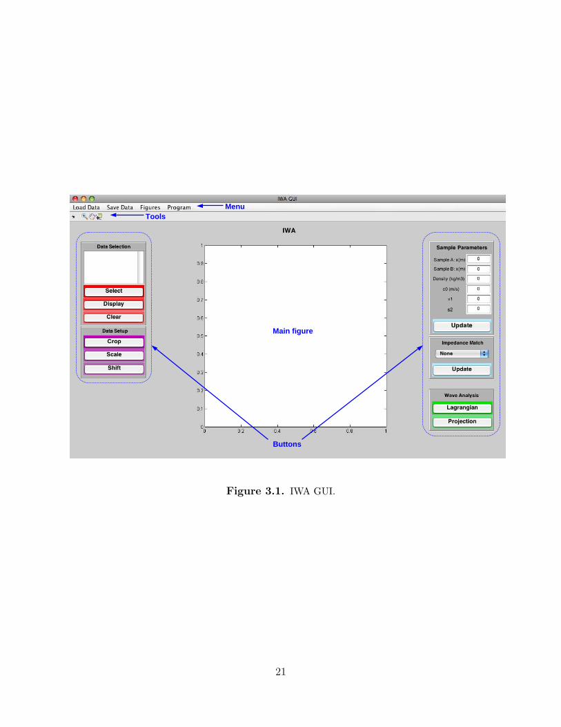
MenuTools

Main figure

Buttons

Figure 3.1. IWA GUI.

21

Under the Save Data menu heading, the “Store Data” and “Export Data” actions areenabled. The store data action saves the analyzed results into data matrices. The exportdata action takes the stored data matrices and exports them as ASCII text files into thedirectory that the user chooses.

Under the Figures menu heading, individual plots may be opened in separate figurewindows. The figures can be saved to a file using the “Save figure” button (disk icon) of thefigure window. The default format is a MATLAB figure (.fig), but other formats (.pdf, .eps,.jpg, .tif, etc.) are available.

Under the Program menu heading, the following actions are enabled: “About”, “Restart”,and “Exit”. The about action provides general information about IWA. Restart closes andrelaunches the program, clearing all parameters and returning the program to its defaultstate. Exit closes the program.

3.2.4 Tools items

Under the Menu bar is the “Tools” bar, which contain tools to aid the user in the analysis.

1. “Zoom” - plots can be zoomed into with either a left mouse click or by clicking anddragging to create a zoom box. Shift-click zooms out and double click restores the plotto the original view. Press the right mouse button for additional options.

2. “Pan” - user can click and drag the plot around for better viewing.

3. “Data cursor” - displays the (x, y, z) values of the point that the user clicks on. Right-click for additional options.

3.3 Analysis overview

The analysis stages of the IWA program are displayed in Fig. 3.2.

3.3.1 Load data

The IWA program begins by opening the load data menu. The first step is to set thedirectory for importing and exporting files. Next, the data files are imported individuallyinto the program. The first column of each file should be the time points, and the secondcolumn should be the velocity points.

22

LoadData

DataSelection

DataSetup

SampleParameters

WaveAnalysis

SaveData

ImpedanceMatch

Figure 3.2. IWA layout.

23

3.3.2 Data selection

The “Data Selection” panel consists of a file viewer window and three action buttons: “Se-lect”, “Display”, and “Clear”. To begin the user clicks on the file viewer window to showthe names of all loaded files. To choose a data file, the user clicks on the name of the datafile and then clicks on the select button. Next, to view the data in the main figure window,the user clicks on the display button. Additional data may be chosen by subsequent clickingon file names and the select button. The velocity profiles are numerically labelled based onorder of selection. Alternatively, multiple sets of data may chosen by highlighting all of thedesired file names and clicking on the select button. To remove all of the selected data, theuser clicks on the clear button, and new data selection can be done.

3.3.3 Data setup

The “Data Setup” panel consists of the action buttons: “Crop”, “Scale”, and “Shift”. Tobegin, the user clicks on the crop button to choose the time range of interest. Since, thesubsequent analysis stages are performed with SI (mks) units, the data need to be convertedsuch that velocity is in m/s and time in s. Upon clicking the scale button, the user is askedto scale either the velocity or time values. Next, the user is asked if the scaling will beperformed on all of the data at once with a single scale factor or separately with individualscale factors. In a similar manner, shifting of the velocity profiles along the time or velocityaxis is performed by clicking on the shift button.

3.3.4 Sample parameters

The “Sample Parameters” panels consists of 6 input boxes and the “Update” button. Thetop 2 boxes are for the thicknesses (m) of the 2 samples (A and B) to be compared. Theother boxes are for the sample density (kg/m3), initial bulk wave velocity c0 (m/s), first orderwave velocity parameter s1, and second order wave velocity parameter s2. The Lagrangianwave velocity of the sample is assumed to be the form,

c ≈ c0 + s1up + s2u2p. (3.1)

After inputing the sample parameters, the user clicks on the update button to set the valuesinto the program.

3.3.5 Impedance match

The “Impedance Match” panel consists of a drop down list and the “Update” button. Thefunction of this action is to convert the measured interface velocity profiles into in-situ

24

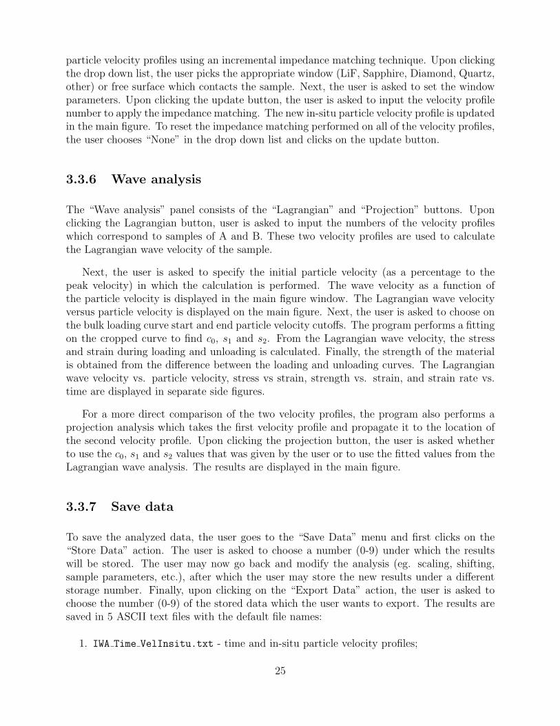
particle velocity profiles using an incremental impedance matching technique. Upon clickingthe drop down list, the user picks the appropriate window (LiF, Sapphire, Diamond, Quartz,other) or free surface which contacts the sample. Next, the user is asked to set the windowparameters. Upon clicking the update button, the user is asked to input the velocity profilenumber to apply the impedance matching. The new in-situ particle velocity profile is updatedin the main figure. To reset the impedance matching performed on all of the velocity profiles,the user chooses “None” in the drop down list and clicks on the update button.

3.3.6 Wave analysis

The “Wave analysis” panel consists of the “Lagrangian” and “Projection” buttons. Uponclicking the Lagrangian button, user is asked to input the numbers of the velocity profileswhich correspond to samples of A and B. These two velocity profiles are used to calculatethe Lagrangian wave velocity of the sample.

Next, the user is asked to specify the initial particle velocity (as a percentage to thepeak velocity) in which the calculation is performed. The wave velocity as a function ofthe particle velocity is displayed in the main figure window. The Lagrangian wave velocityversus particle velocity is displayed on the main figure. Next, the user is asked to choose onthe bulk loading curve start and end particle velocity cutoffs. The program performs a fittingon the cropped curve to find c0, s1 and s2. From the Lagrangian wave velocity, the stressand strain during loading and unloading is calculated. Finally, the strength of the materialis obtained from the difference between the loading and unloading curves. The Lagrangianwave velocity vs. particle velocity, stress vs strain, strength vs. strain, and strain rate vs.time are displayed in separate side figures.

For a more direct comparison of the two velocity profiles, the program also performs aprojection analysis which takes the first velocity profile and propagate it to the location ofthe second velocity profile. Upon clicking the projection button, the user is asked whetherto use the c0, s1 and s2 values that was given by the user or to use the fitted values from theLagrangian wave analysis. The results are displayed in the main figure.

3.3.7 Save data

To save the analyzed data, the user goes to the “Save Data” menu and first clicks on the“Store Data” action. The user is asked to choose a number (0-9) under which the resultswill be stored. The user may now go back and modify the analysis (eg. scaling, shifting,sample parameters, etc.), after which the user may store the new results under a differentstorage number. Finally, upon clicking on the “Export Data” action, the user is asked tochoose the number (0-9) of the stored data which the user wants to export. The results aresaved in 5 ASCII text files with the default file names:

1. IWA Time VelInsitu.txt - time and in-situ particle velocity profiles;

25

2. IWA TimeSR StrainRate.txt - time and strain rate;

3. IWA Up Cs Strain Stress.txt - particle velocity, Lagrangian wave velocity, strain,and stress;

4. IWA Strain Strength.txt - strain upon unloading and material strength;

5. IWA TimeProj VelProj.txt - projected time and velocity profile.

26

Chapter 4

Using IWA

This chapter describes the practical use of the IWA program. Analysis of an example isgiven with step-by-step results for comparison. Also, some analysis hints are presented toaid the user.

4.1 Example

The example is taken from a experiment performed on the Veloce pulsed power generator [20,21]. The load consisted of Al 6061-T0 and Al 6061-80 samples, each backed by 6 mm thickLiF windows, that were glued onto 20 mm wide by 1.0 mm thick Al load panels. Ramploading up to 6.5 GPa of the samples was achieved upon discharging the 440 ns, 2.5 MAcurrent pulse of the Veloce generator.

The 4 velocity profiles provided with the IWA package are found in the folder IWAexample:

1. Al LANL 1.4141mm.txt - Al 6061-T0 sample (1.4141 mm thick) with LiF window;

2. Al LANL 2.4011mm.txt - Al 6061-T0 sample (2.4011 mm thick) with LiF window;

3. Al WSU 1.5024mm.txt - Al 6061-80 sample (1.5024 mm thick) with LiF window;

4. Al WSU 2.4023mm.txt - Al 6061-80 sample (2.4023 mm thick) with LiF window.

After setting the directory to where the data files are located, load each file with the loaddata action. Next, in the data selection panel click on the file viewer window and highlightall of the file names. After clicking the select and display button, the velocity profiles shouldbe displayed in the main figure, as shown in Fig. 4.1.

Under the data setup panel, click on the crop button to limit the data range from t =900 ns to 1850 ns. Use the scale button to convert the units of the velocity (km/s) and time(ns) data points to m and s, respectively. The cropped and scaled velocity profiles shouldbe now resemble Fig. 4.2.

The following steps correspond specifically to the analysis of the Al 6061-T0 data set,namely velocity profiles 1 and 2. Under the sample parameters panel, set the thickness of

27

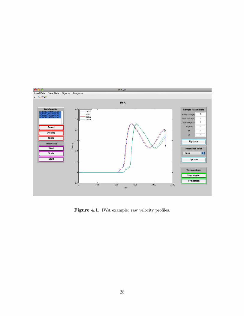
Figure 4.1. IWA example: raw velocity profiles.

28

Figure 4.2. IWA example: cropped and scaled velocityprofiles.

29

sample A and B to 1.4141e-3 m and 2.4011e-3 m, respectively. Also, set the sample densityto 2.700e3 kg/m3, c0 = 5.288e3 m/s, s1 = 2.752 and s2 = 0. Click on the update button toset the values into the program.

Since these samples are backed by LiF windows, under the impedance match panel setthe window material to “LiF”. To perform the incremental impedance matching, click on theupdate button and enter number “1” to convert the first raw velocity profile to an in-situparticle velocity profile. Repeat the updating on the rest of the raw velocity profiles (i.e. 2,3, 4) until all are converted to in-situ particle velocity profiles, which should now resembleFig. 4.3.

Under the wave analysis panel, click on the Lagrangian button and enter velocity profilenumbers “1” and “2” for the inputs of samples A and B, respectively. After the Lagrangianwave velocity plot appears in the main figure, click on start and end points on the bulkloading curve. Since these points are used define the data range in which the program fitsthe material’s bulk response, avoid the initial elastic wave velocity and the bending sectionnear peak loading. The fitted curve along with the linear fit parameters c0, s1 and s2 aredisplayed in the main figure, as shown in Fig. 4.4.

From the Lagrangian wave velocity, the program calculates the loading and unloadingstress-strain curves which are then used to obtain the material’s strength as a function ofunloading strain. Also, the strain rate as a function of time is calculated by the program.These results are displayed in separate side figures, as shown in Fig. 4.5.

To compare the velocity profile of sample A projected forward to the sample B location,click the projection button. Enter velocity profile numbers “1” and “2” for the inputs ofsamples A and B, respectively. The user is asked which sample parameter, the “Fit” valuesobtained from the analysis or the original “Given” values that the user previously inputtedinto the program. The projected velocity profile is shown in Fig. 4.6.

At this point, the user may want to input the new “fitted” values of c0, s1 and s2 into thesample parameters boxes and update their values. Repeat the impedance matching to get anew set of in-situ velocity profiles, and the perform the Lagrangian and projection analysisagain. The process may be repeated until the user is satisfied with that the input sampleparameters and fitted parameters are consistent with each other.

Under the save data menu, store the analyzed results as storage number “1”. The usermay now export the results using the export data action. The results are saved as 5 ASCIItext files in the directory chosen by the user. Alternatively, the user may perform additionalanalysis such as analyzing the Al 6061-80 data set (velocity profiles 3 and 4). Those resultsmay be stored under a different storage number and exported.

30

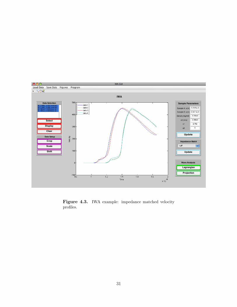
Figure 4.3. IWA example: impedance matched velocityprofiles.

31

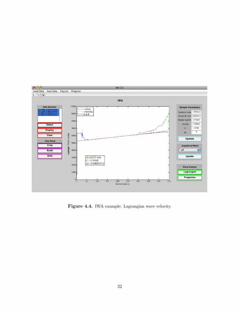
Figure 4.4. IWA example: Lagrangian wave velocity.

32

(a) (b)

(c)

(d)

Figure 4.5. IWA example: side figures of (a) Lagrangianwave velocity vs. particle velocity, (b) stress vs. strain, and(c) strength vs. strain (d) strain rate vs. time.

33

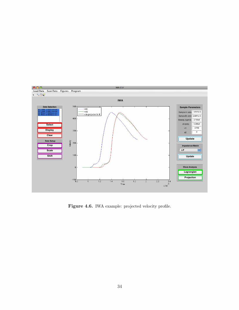
Figure 4.6. IWA example: projected velocity profile.

34

4.2 Analysis hints

4.2.1 Cropping

The current IWA program is not setup for reloading profiles. In the above example, afterthe unloading the data was cropped prior to the reloading of the upstream velocity profile.Also, at the start of the Lagrangian wave analysis, an initial velocity cutoff (% of the peakvelocity) is chosen to avoid the noisy signal at the low velocities which would cause spikesin wave velocity calculations.

4.2.2 Smoothing

After the raw data is cropped to the appropriate data range, an initial smoothing parameteris selected to reduce noise effects in the analysis. The precise choice will depend on the levelof signal noise, the sampling rate, and the relevant features of interest.

4.2.3 Scaling

Intuitively, the downstream velocity profile should have lower peak velocity than the up-stream velocity profile. However, due to non-uniform drive along the panel the downstreampeak velocity might be higher the upstream peak velocity. For that case, the downstreamvelocity profile should be scaled lower so its peak is the same or less than the upstream peakvelocity.

35

36

Chapter 5

Summary

5.1 Program features

The IWA program accepts measured velocity profiles from isentropic compression experi-ments in the form of separate text files. The user may scale and shift the data, and specifythe time range over which the analysis is performed. Sample parameters are entered directlyinto the program and may be changed during the analysis. Incremental impedance matchingis performed to convert measured velocity profiles to in-situ particle velocity profiles.

Lagrangian wave analysis is performed to obtain the Lagrangian wave velocity, stress,strain, strain rate, and strength of the material. In addition, velocity profiles at upstreammaterial positions may be projected forward and compared with downstream velocity pro-files. Results generated by IWA may be exported as text files for post-processing or be savedin various graphical formats.

5.2 Future releases

Users should contact Tommy Ao (tao@sandia.gov) with questions, bug reports, and featurerequests. Bug fixes will be made as necessary and will be distributed by email. Featuresunder consideration for future versions of IWA include:

• Recall configurations of previous settings and results, and

• Single velocity profile approximate analysis.

No scheduled update to IWA is planned at this time, but new releases will be consideredbased on user feedback.

37

38

References

[1] R. G. McQueen, S. P. Marsh, J. W. Taylor, J. N. Fritz, and W. J. Carter, “The equationof state of solids from shock wave studies,” in High-Velocity Impact Phenomena (R.Kinslow, ed.), (New York), pp. 249–417, Academic Press, 1970.

[2] R. J. Trainor, J. W. Shaner, J. M. Auerbach, and N. C. Holmes, “Ultrahigh-pressurelaser-driven shock-wave experiments in aluminum,” Physical Review Letters, vol. 42,no. 17, pp. 1154–1157, 1979.

[3] A. C. Mitchell and W. J. Nellis, “Shock compression of aluminum, copper, and tanta-lum,” Journal of Applied Physics, vol. 52, no. 5, pp. 3363–3374, 1981.

[4] C. E. Ragan, III, “Shock-wave experiments at three-fold compression,” Physical ReviewA, vol. 29, no. 3, pp. 1391–1402, 1984.

[5] L. M. Barker and R. E. Hollenbach, “Shock-wave studies of PMMA, Fused Silica, andSapphire,” Journal of Applied Physics, vol. 41, no. 10, pp. 4208–4226, 1970.

[6] J. H. Nguyen, D. Orlikowski, F. H. Streitz, J. A. Moriarty, and N. C. Holmes, “High-pressure tailored compression: Controlled thermodynamic paths,” Journal of AppliedPhysics, vol. 100, no. 2, p. 023508, 2006.

[7] J. Edwards, K. T. Lorenz, B. A. Remington, S. Pollaine, J. Colvin, D. Braun, B. F.Lasinski, D. Reisman, J. M. McNaney, J. A. Greenough, R. Wallace, H. Louis, andD. Kalantar, “Laser-driven plasma loader for shockless compression and acceleration ofsamples in the solid state,” Physical Review Letters, vol. 92, no. 7, p. 075002, 2004.

[8] J. R. Asay, “Isentropic compression experiments on the Z Accelerator,” in Shock Com-pression of Condensed Matter-1999 (M. D. Furnish, L. C. Chhabildas and R. S. Hixson,ed.), (New York), p. 261, AIP, 2000.

[9] J. R. Asay and M. D. Knudson, “Use of pulsed magnetic fields for quasi-isentropic com-pression experiments,” in High-Pressure Shock Compression of Solids VIII: The Scienceand Technology of High-Velocity Impact (L. Chhabildas, L. Davison, and Y. Horie, eds.),p. 329, 2005.

[10] J. L. Ding and J. R. Asay, “Material characterization with ramp wave experiments,”Journal of Applied Physics, vol. 101, no. 7, p. 073517, 2007.

[11] J. B. Aidun and Y. M. Gupta, “Analysis of Lagrangian gauge measurements of simpleand nonsimple plane waves,” Journal of Applied Physics, vol. 69, no. 10, pp. 6998–7014,1991.

39

[12] L. Davison and R. A. Graham, “Shock compression of solids,” Physics Report, vol. 55,pp. 255–379, 1979.

[13] J. R. Asay and G. I. Kerley, “The response of materials to dynamic loading,” Int. J.Impact Engng, vol. 5, pp. 69–99, 1987.

[14] L. C. Chhabildas and L. M. Barker, “Dynamic quasi-isentropic compression of tung-sten,” in Shock Waves in Condensed Matter-1987 (S.C. Schmidt and N.C. Holmes, ed.),(New York), p. 111, Elsevier, 1988.

[15] G. R. Fowles, “Shock wave compression of hardened and annealed 2024 aluminum,”Journal of Applied Physics, vol. 32, no. 8, p. 1475, 1961.

[16] J. R. Asay and J. Lipkin, “A self-consistent technique for estimating the dynamicyield strength of a shock-loaded material,” Journal of Applied Physics, vol. 49, no. 7,pp. 4242–4247, 1978.

[17] J. R. Asay, D. Dandekar, and L. C. Chhabildas, “Shear strength of shock-loaded poly-crystalline tungsten,” Journal of Applied Physics, vol. 51, no. 9, p. 4774, 1980.

[18] T. J. Vogler and L. C. Chhabildas, “Strength behavior of materials at high pressures,”Int. J. Impact Engng, vol. 33, p. 812, 2006.

[19] H. Huang and J. R. Asay, “Reshock and release response of aluminum single crystal,”Journal of Applied Physics, vol. 101, no. 6, p. 063550, 2007.

[20] T. Ao, J. R. Asay, S. Chantrenne, M. R. Baer, and C. A. Hall, “A compact strip-linepulsed power generator for isentropic compression experiments,” Review of ScientificInstruments, vol. 79, p. 013903, 2008.

[21] J. R. Asay, T. Ao, J.-P. Davis, C. Hall, T. J. Vogler, and I. G. T. Gray, “Effect of ini-tial properties on the flow strength of aluminium during quasi-isentropic compression,”Journal of Applied Physics, vol. 103, p. 083514, 2008.

40

DISTRIBUTION:

1 MS 0826 W. M. Trott, 1512

1 MS 0836 M. R. Baer, 1500

10 MS 1106 T. Ao, 1646

1 MS 1159 S. C. Jones, 1344

1 MS 1189 M. P. Desjarlais, 1640

1 MS 1189 T. A. Mehlhorn, 1640

1 MS 1195 J. R. Asay, 1646

1 MS 1195 C. S. Alexander, 1646

1 MS 1195 J.-P. Davis, 1646

1 MS 1195 D. H. Dolan, 1646

1 MS 1195 M. D. Furnish, 1646

1 MS 1195 C. A. Hall, 1646

1 MS 1195 R. J. Hickman, 1646

1 MS 1195 M. D. Knudson, 1646

1 MS 1195 S. Root, 1646

1 MS 1195 W. D. Reinhart, 1646

1 MS 1195 J. L. Wise, 1646

1 MS 9042 T. J. Vogler, 8776

1 MS 0899 Technical Library, 9536 (electronic copy)

41

42