jackd/stat305/wk02-1.docx · web viewstat 305 week 2 notes wk 2 – hrs 1-2 (mon, sept 12) review...

Stat 305 Week 2 Notes

Wk 2 – Hrs 1-2 (Mon, Sept 12) Review of fundamentals, specifically sampling methods.

Wk 2 - Hr 3 (Wed, Sept 14): Probability and disease diagnostics, conditional probability, marginal, and Bayes rule

Stat 305 Notes. Week 2, / 93

My friend Dave has terrible luck. He bought a computer, and within 11 months (still under warranty) he had replaced the… … bluetooth (twice), …motherboard, …heat sink, fans, and “media button bar” (twice), …hard drive (four times!) …and his company loyalty.


After that, they replaced the computer completely and the new one works fine, I think.

When a product is a dud, it’s expensive. To limit risks a company needs to know the chances of a product failure or not being the advertised weight.


The computer company needs to know the chances (probability) that a laptop will fail in the first 1, 2, or 3 years.

On a $1500(ish) laptopStat 305 Notes. Week 2, / 93

• Dell offers 1 year ‘free’ basic warranty.

• Extend the warranty to 2 years $160

• Extend the warranty to 3 years for $230

• Extend the warranty to 4 years for $370


The chance of costly repairs increases with time, so the price of the warranties goes up as they get longer. The company still needs to make money, knowing the chance of failure sets the price. Stat 305 Notes. Week 2, / 93

Knowing the probability of a repair means that they can set the price to, on average, pay out less than they charge for warranty costs.

• Some machines won’t incur costs

• Other machines are doomed to eat company profits


Probability is the likelihood of a specific event out of all possible events • Probability =

Number of times a specific event can occur ÷ by Total Number of times that any event can occur. (this is an important slide)


Example: Ratio of the number of computers that fail out of the number of computers produced. Pr(failure in year 1) = 32 Million Failed Computers ---------------------------- 500 Million Computers Pr(failure in year 1) = 32 / 500 = 6.4% (So that ‘free’ warranty costs the company 6.4% of the repair cost)


Example: Roll up the Rim. Pr(WINNER!) = Winning cups / Total cups


(In 2011) There were 45 million winning cups And 270 million cups in total


Pr(WINNER!) = 45 million / 270 million

= 1/6 … just as advertised.

Probability is always between 0 and 1, inclusive. Stat 305 Notes. Week 2, / 93

If something never happens, it has zero probability. Pr(winning an angry raccoon) = 0 cups / 270 million 0 / anything = 0. Pr(winning an angry raccoon) = 0

If something is certain to happen it has probability one. Stat 305 Notes. Week 2, / 93

Pr(the cup was red) = 270 million / 270 million Anything divided by itself is one. We’re also assuming complete randomness. That means that every cup is equally likely. If you know the winning cups in advance, Pr(you winning) is not 1/6. Random is not the same as haphazard, spontaneous, or crazy. Pointing out things like this out a lot will help if you have too many friends.


Probability is the long term proportion of events of interest to the total number of all possible events that occur. Example: Flip a coin. Pr(heads) = Times a coin comes up heads… EVER!! --------------------------------------------------------- Times a coin is flipped…. EVER!! Assume all coins are the same, this probability should come

up as ½


An event either happens or it doesn’t. This is certain. That means the chance of an event either happening or not

happening is 1. We can use this to find the chance of something not happening. Pr(Winning cup) + Pr(Losing cup) = 1 So Pr(Losing cup) = 1 – Pr(Winning cup)


Pr(Losing cup) = 1 – 1/6 (or 6/6 – 5/6)

= 5/6

If one in every six cups is a winner. Then the other five cups in six are losers.

In general, the converse law is:


(this is important)

You can find the probability of more complex events by composing them of simpler events.

If two events are independent, meaning they don’t affect each other, then the chance of BOTH of them happening is two probabilities multiplied.

Pr( Winning cup AND flipping a coin heads) = 1/6 x 1/2 = 1/12


Example: Cards

In standard deck of 52 cards, there are 4 suits and 13 ranks. Suit and rank are independent.

Pr(Ace of Spades) = Pr(Ace) x Pr(Spade)

= 1 rank /13 ranks x 1 suit / 4 suits

= 1/13 x 1/4

= 1/52

There is 1 Ace of Spades in a deck of 52 cards.

The (simplified) rule for two events happening together is a multiplication.


Pr(A and B) = Pr(A) x Pr(B) When A and B are independent.


Sometimes events A and B happening together is written as A O B.

The ‘O’ stands for ‘intersect’,

and A O B is the intersection of A and B.

Think of A and B as roads. The intersection is the portion of land that is part of both roads at the same time.


<break>


So what happens when two events are NOT independent?

To answer that, we first have to introduce the concept of conditional probability.

Pr(A | B) is the probability of A GIVEN event B.

In other words, it's the chance of A, conditional on B.

Or, 'if we know B has happened / will happen for sure, what are the chances of A also happening?'


Example: Let's say you miss 10% of your classes, usually.The unconditional (or marginal) probability of missing a day of class/work is:

Pr( miss a day) = 0.10

Being sick will increase the chance that you miss a day of work or class, so we would expect the conditional probability to be higher than the marginal.

Pr( miss a day | sick) = 0.47


Also, the marginal probability accounts for all days, sick or not. Therefore, the chance of missing a day if you're not sick has to be less than the marginal.

Pr( miss a day | NOT sick) = 0.07

Now, let's say you're sick about 5% of the time.

What's the chance on any particular day that you're sick AND you miss the day?Stat 305 Notes. Week 2, / 93

Pr( miss AND sick) = ???It isn't Pr(miss) x Pr(sick), why not?

Multiplying the marginal probabilities won't work because the events (miss a day) and (sick a day) are NOT independent.

These events affect each other.

However, you CAN use a conditional probability.

Pr(miss AND sick) = Pr( sick ) x Pr( miss | sick) = 0.05 x 0.47 = 0.0235


You can read Pr( sick ) x Pr( miss | sick) as...The chance you are sick, and given that, that you miss a day.

You can also represent conditional outcomes in a tree:


The full formula for finding the probability of two events together is:

Pr(A and B) = Pr(A) x Pr(B | A)

or

Pr(A and B) = Pr(B) x Pr(A | B)

because the labels for events are arbitrary.


This formula also works to find the conditional probability.

Pr(B | A) = Pr(A and B) / Pr(A)

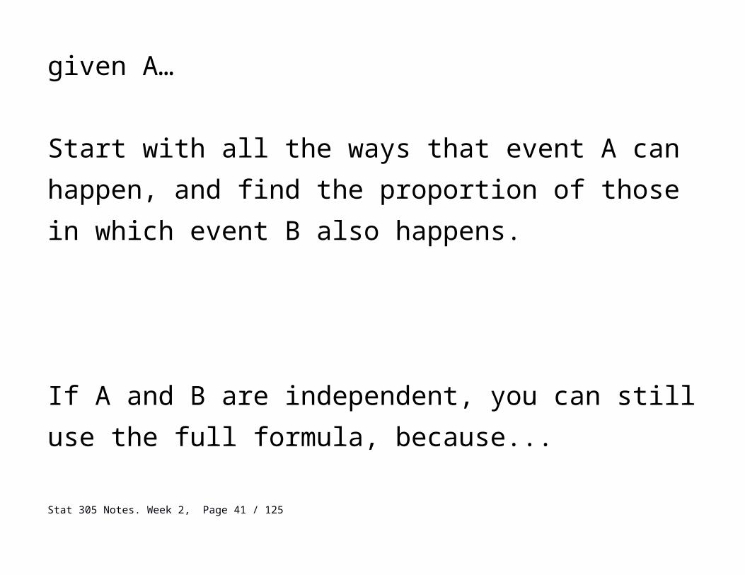
That is, to find the chance of event B given A…

Start with all the ways that event A can happen, and find the proportion of those in which event B also happens.


If A and B are independent, you can still use the full formula, because...

Pr(B | A) = Pr(B) when A and B are independent.

So Pr(A) x Pr(B) and Pr(A) x Pr(B | A)

are the same thing.


Example: A patient has arrived at a clinic. Event D represents that the patient has a certain disease.

Let Pr(D) = 0.12

then...Pr(D | they have a hat) = 0.12

Pr(D | the price of beans in Mongolia are down) = 0.12

but...Pr(D | Tested positive for disease) > 0.12


(advanced) The probability of three or more events can be calculated similarly

Simplified:

Pr(A and B and C) = Pr(A) x Pr(B) x Pr(C) if A,B, and C are independent

Full:Pr(A and B and C) = Pr(A) x Pr(B | A) x Pr( C | A and B)


<break question 1>

Let T be the event that someone tests positive for a disease.Let D be the event that they have the disease.

We would assume that having a disease makes you more likely to test positive. So letPr(T | D) = 0.90Pr(T | not D) = 0.30 , and finallyPr(D) = 0.20

What is the probability of Test pos. AND have disease?


<break question 2>

The chance that a test is positive when someone has a disease is called the sensitivity of the test.

Given againPr(T | D) = 0.90Pr(T | not D) = 0.30, and finallyPr(D) = 0.20

What is the sensitivity of this test?


<break question 3>

The chance that a test is negative when someone does NOT have a disease is called the specificity of the test.

Given againPr(T | D) = 0.90Pr(T | not D) = 0.30 , and finallyPr(D) = 0.20

What is the specificity of this test?We will return to these concepts later.Stat 305 Notes. Week 2, / 93

The intercept / ‘Or’ operator.

If we take two events that never happen together , the probability of one event OR the other happened is the two probabilities added together.

Pr( Vancouver OR Toronto is voted the best city) = Pr( Vancouver is best) + Pr(Toronto is best)

They can’t both be the best city, so these events never happen together.


Another term for ‘never happening together’ is mutually exclusive.

Example: A lottery machine picks a single number from 1 to 49.

Pr( Machine picks 1 or 2) =

Pr( Picks 1) + Pr(Picks 2)

= 1/49 + 1/ 49 = 2/49

The (simplified) one-or-the-other formula is... Stat 305 Notes. Week 2, / 93

Pr(A OR B) = Pr(A) + Pr(B)

… when A or B can’t happen together.

We could also have written Pr( Picks 2 or less) = 2/49 For that matter, we could have written… Pr( Picks 3 or less) = Pr(Picks 1) + Pr(Picks 2) + Pr(Picks 3) = 1/49 + 1/49 + 1/49 = 3/49


Can you guess: Pr( Machine picks 10 or less)

10 numbers that are 10 or less 10 ---------------------------------------- = ------- 49 numbers in total 49

(A machine picks a single number from 1 to 49)

How about…


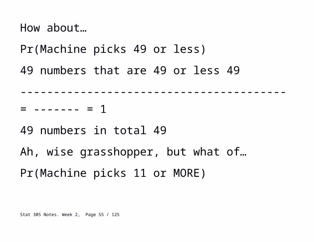
Pr(Machine picks 49 or less)

49 numbers that are 49 or less 49

---------------------------------------- = ------- = 1

49 numbers in total 49

Ah, wise grasshopper, but what of…

Pr(Machine picks 11 or MORE)

Pr(11 or more) = 1 – Pr(10 or less) = 1 – 10/49 = 39/49

(Hint: use previous two answers)


<break>


What happens when the two events are CAN happen together?

In other words, what happens when events A and B are NOT mutually exclusive?

We can't just add the chance of the two events because some events are going to get double counted.


By example, in a 52 card deck of cards, what is the chance of getting a King OR a Heart.

There are 4 kings, and there are 13 hearts.

But there are only 16 cards that either a king OR a heart.

A , 2 , 3 , 4 , 5 , 6 , 7 , 8

9 , 10 , J , Q , K , K , K , .... K


If we were to add the probabilities as if they were mutually exclusive, we would over estimate the total probability.

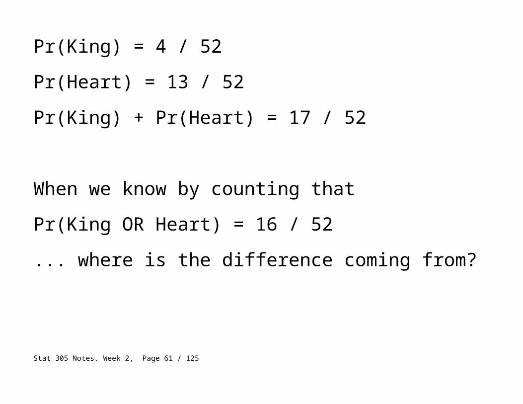
Pr(King) = 4 / 52

Pr(Heart) = 13 / 52

Pr(King) + Pr(Heart) = 17 / 52

When we know by counting that

Pr(King OR Heart) = 16 / 52

... where is the difference coming from?Stat 305 Notes. Week 2, / 93

If we add the two possibilities directly, the king of hearts is counted in both sets.

A , 2 , 3 , 4 , 5 , 6 , 7 , 8

9 , 10 , J , Q , K

K , K , K , .... KStat 305 Notes. Week 2, / 93

The FULL formula for finding Pr(A or B) is...

Pr(A or B) = Pr(A) + Pr(B) – Pr(A and B)

where Pr(A) + Pr(B) is getting the outcomes from both sets, and - Pr(A and B) one copy of each 'double counted' outcome.

Pr(King or Heart) = 4/52 + 13/52 – 1/52


If you don't know if two events are mutually exclusive, which formula is used?

Always use the full formula.

If A and B are mutually exclusive, then Pr(A and B) = 0, therefore subtracting Pr(A and B) won't change anything.

The 'addition only' formula is just a convenient shortcut.

<break question 1>

Two six-sided dice are rolled. (Rolls are independent)


Pr( First die rolls a 3) =


<break question 2>


Pr( Both dice roll 3s) =


Now for the true test of a warrior’s spirit: <break question 3>


Pr( At least one die rolls a 5) =


(Notice we have an extra step in finding the 'both' chance)In case you were wondering, there are dice of other than six-sides. (for interest)


Guess why the one on the right is bad?

Sometimes the collection of events ‘A or B’ is written


‘A U B’.

The ‘U’, stands for ‘union’.

A union is a collection of something, so A U B is the collection of all possible outcomes that are in either event A or B (or both).


We can also combine events into more complex situations like (A and B) or C.

As per order of operations:

Parentheses ( ) define what gets evaluated first.

The intersection / ‘and’ operator is like a multiplier so it takes precedence over the union / ‘or’ operator.

BUT… you should always use ( ) to be clear.


Example: The composite event (A int B) U (A int C)

Can be said “both events A and B, or both events A and C”

It can also be simplified to A int (B U C)


There are a few more special cases with union and intersection, and the probability of events:

Recall that Pr(certain) = 1 and that Pr(impossible) = 0,Where ‘certain’ is all possible outcomes, and ‘impossible’ includes no possible outcomes.

So Pr(A U certain) = 1, because the union includes an event that is certain (all possible events).

Also, Pr(A U impossible) = Pr(A), because the union doesn’t include any possible events that aren’t already in A.Stat 305 Notes. Week 2, / 93

Similarly for intersections:

Pr(A int certain) = Pr(A) because every outcome that’s in A is also in ‘certain’

Pr(A int impossible) = 0 because the intersection of A and impossible (no possible outcomes), cannot contain any outcomes.

Now we have everything we need to discuss…Stat 305 Notes. Week 2, / 93

Law of Total Probability

The law of total probability is an extension of

Pr(A int certain) = Pr(A)

The law states that…

Pr(A int (B1 U B2 U … U BN)) = Pr(A)

…if the events B1 , B2 , … , BN are a partition of all possibilities


A partition is a set of events that are:

1. Mutually exclusive (nothing can be in 2+ events at once)

2. Exhaustive(every possible outcome is in one of the events)

The mutual exclusive part makes applying ‘or’/union very simple.

Example: {A, not A} is a very simple partitionStat 305 Notes. Week 2, / 93

Example 1: How often does a test for disease come up positive?

Let D be the event that someone has a disease, and Let T be the event that a test result is positive.

Pr(D) = 0.25Pr(T | D) = 0.80Pr(T | not D) = 0.10


First, we check for a partition.Every outcome is either part of exactly one of {D, not D}, so we have a partition.

Second, find the intersects

Pr(T int D) = Pr(D) x Pr(T | D) = 0.25 x 0.80 = 0.200

Pr(T int (not D) = Pr(not D) x Pr(T | not D) = 0.75 x 0.10 = 0.075


Finally, we apply the law of total probability:

(T int D) U (T int (not D)) = T int (D U not D) = T

So Pr(T) = Pr( T int D) + Pr( T int (not D)) = 0.200 + 0.075 = 0.275

Note we can apply the simple addition rule because (T int D) and (T int (not D)) are mutually exclusive.


Now let's talk about babies.


<break question 1>

Every baby is going to be born pre-term, normal, or late.

What is the chance that a baby will be born at the normal time?

Pr(Pre-Term) = 0.12Pr(Late) = 0.08


<break question 2>

What is the chance that any given baby will be born underweight AND pre-term?

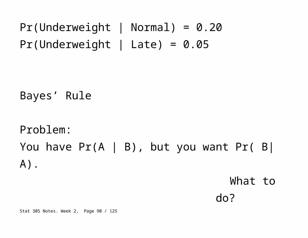
Pr(Pre-Term) = 0.12Pr(Late) = 0.08Pr(Underweight | Pre-Term) = 0.60Pr(Underweight | Normal) = 0.20Pr(Underweight | Late) = 0.05


<break question 3>

What is the chance that any given baby will be born underweight?

Pr(Pre-Term) = 0.12Pr(Late) = 0.08Pr(Underweight | Pre-Term) = 0.60Pr(Underweight | Normal) = 0.20Pr(Underweight | Late) = 0.05


Bayes’ Rule

Problem: You have Pr(A | B), but you want Pr( B|A).

What to do?

We know that:Pr(A int B) = Pr(A) x Pr(B | A)

And that:Pr(A int B) = Pr(B) x Pr(A | B)


So then

P(A) x Pr(B | A) = Pr(B) x Pr(A | B)

And therefore…

P(B|A) = Pr(A | B) * P(B) / P(A)

This is called Bayes’ Rule, and it’s very useful in disease diagnostics.


For example, we may know things like the sensitivity and specificity of a particular test, and we may know the general prevalence of a disease (at least among patients getting tested). This is all information that would be documented and made available by health authorities or test manufacturers.

But what we REALLY want to know on a case-by-case basis is this:

If someone tests positive for a disease, what is the chance that they actually have it?Stat 305 Notes. Week 2, / 93

In mathematical terms, we often have…

Pr(D) (The prevalence of the disease)Pr(T|D) (The sensitivity of the disease)1 – Pr(not T | not D) (The specificity of the disease)

but we want this:

Pr( D | T)

Bayes’ Law makes this straight forward.


Return to some previous quiz questions.

Before, with this information,

Pr(D) = 0.25Pr(T | D) = 0.80Pr(T | not D) = 0.10

We found that Pr(T), the chance of a positive test wasPr(T) = 0.275

…using the Law of Total Probability.Stat 305 Notes. Week 2, / 93

A patient comes in and tests positive for this disease. What is the chance that they actually have it?

As per Bayes’ rule.

Pr(D | T) = Pr(D) / Pr(T) x Pr(T|D)

= 0.25 / 0.275 x 0.80 = 0.7273.

Is this enough for a diagnosis? What if we repeated the test?


The test is repeated and comes up positive again. Assuming each test is independent, what are the chances that patient has the disease given both of these tests?

Let T1 and T2 be positive results from each test, respectively.

Pr(T1 | D) = 0.80, Pr(T2 | D) = 0.80SoPr(T1 int T2 | D) = 0.64

LikewisePr(T1 int T2 | not D) = 0.10 x 0.10 = 0.01Stat 305 Notes. Week 2, / 93

Next get the probabilities of the intercept.

Pr(T1 int T2 int D) = Pr(D) x Pr(T1 int T2 | D) = 0.25 x 0.64 = 0.1600

Pr(T1 int T2 int (not D)) = Pr(not D) x Pr(T1 int T2 | D) = 0.75 x 0.01 = 0.0075


Now apply the law of total probability.

Pr(T1 int T2) = Pr(T1 int T2 int D) + Pr(T1 int T2 int (not D))

= 0.1600 + 0.0075= 0.1675

Finally, Bayes’ RulePr(D | T1 int T2) = Pr(D) / Pr(T1 int T2) x Pr(T1 int T2 | D)

= 0.25 / 0.1675 x 0.64= 0.9552


It's a lot, but I'm sure you can digest it.


A few parting comments and ROC curves.


Pr( D | one test positive) = 0.7273Pr( D | two tests positive) = 0.9552

So with one test, we can get a decent indication of someone’s disease status, but nothing definitive.

Two tests work a lot better than one, if, AND THIS IS A BIG IF, the tests are independent.

A lot of times the reason behind a false positive can continue from test to test. In that case, repeating a test will make less of an improvement, if any.Stat 305 Notes. Week 2, / 93

Also, consider the different parts of the Bayes’ Rule formula.

Pr(D | T) = Pr(D) / Pr(T) x Pr(T|D)

The perfect test would be one where the Pr(D | T) = 1 and where Pr(D | not T) = 0.

What contributes to a high Pr(D| T) ?- A common disease ( Pr(D) large)- A sensitive test ( Pr(T|D) large), and- A small Pr(T).


But where does Pr(T) come from?

Recall that Pr(T) = Pr( T int D) + Pr( T int (not D))

A large Pr(T int D) would come from a high sensitivity (and disease prevalence), and

A small Pr(T int (not D)) would come from a high specificity.

So the quality of the information we get from a test comes from the rates of true positives and of false positives.ROC Curves.Stat 305 Notes. Week 2, / 93

Sensitivity and specificity represent a trade-off between priorities.

If it’s very important to detect a disease, then a high sensitivity is desirable. (e.g. in the case of something infectious, or something with good early treatment options)

If it’s very important to be sure about a disease, specificity is important. (e.g. if a treatment is dangerous, or otherwise detrimental)Some tests can be calibrated to sacrifice some specificity for Stat 305 Notes. Week 2, / 93

better sensitivity, or vice versa.

Example: Consider HIV. One common test of HIV is to look for low counts of CD4 in the blood. The lower the CD4, the greater chance of infection (and the weaker the immune system).

We can decide what the cut-off should be for deciding if a test for HIV is positive or not.

A ‘receiver operator characteristic’ (ROC) curve is one that Stat 305 Notes. Week 2, / 93

shows you what the sensitivity of your test would be at different levels of specificity.

Using such a curve, you can make an informed answer about your cutoff.

The following image is an ROC curve from a study on CD8 counts on detecting Tuberculosis co-infections with HIV.

Article Source: Hierarchy Low CD4+/CD8+ T-Cell Counts and IFN-γ Responses in HIV-1+ Individuals Correlate with Active TB and/or M.tb Co-Infection Shao L, Zhang X, Gao Y, Xu Y, Zhang S, et al. (2016) Hierarchy Low CD4+/CD8+ T-Cell Counts and IFN-γ Responses in HIV-1+ Individuals Correlate with Active TB and/or M.tb Co-Infection. PLoS ONE 11(3): e0150941. doi: 10.1371/journal.pone.0150941


http://journals.plos.org/plosone/article?id=10.1371%2Fjournal.pone.0150941

http://journals.plos.org/plosone/article?id=10.1371%2Fjournal.pone.0150941

In this image, we can see that in order to reach 60% sensitivity, we can get at most 80-88% specificity.

To get 80% sensitivity, we would need to accept specificity of about 60%.


The straight diagonal line (dashed in your textbook) represents the ‘random guess line’. Ideally, you should pick a point on the curve far above this line.

Along this line, your test is just as good as a random guess. Along this line, the sensitivity is the same as the specificity, or

Pr(T|D) = Pr(T | not D)

Meaning the test will give the same answer regardless of disease status. Stat 305 Notes. Week 2, / 93

(advanced) The ROC curve in your textbook (Page 142, 2nd edition), is smoothed out to represent what the ROC curve could look like if you have thousands of data points.

In academic literature, most ROC curves are shown as jagged lines, where each step up represents a data point.Stat 305 Notes. Week 2, / 93

(advanced) Finally, the AUC stands for “area under curve”, which is literally the area of the shape under the ROC curve.

A perfect test has an AUC of 1.

A random guess has an AUC of 0.5.Stat 305 Notes. Week 2, / 93

Linking up to Hypothesis testing

You have already seen the mechanics of this trade-off between sensitivity and specificity before, in another context.

What if we assume that a patient is healthy until there is sufficient evidence otherwise? Then we would call the event that a patient is healthy, (not D), the null hypothesis.


Treating (not D) as the null hypothesis, then…

- Pr(T | D) is the power of the diagnostic test, and - Pr(not T | D) is beta, the change of a Type II error.

- Pr(not T | not D) is alpha, the chance of a Type I error.

In other terms:Specificity would be the significance level alpha, and Sensitivity is the power of the test, 1 - beta.


On the issue of sampling of patients

Previously, we linked the marginal chance of a disease, Pr(D), to the prevalence of a disease, but there’s a big practical issue with this:

Pr(D) is the proportion of a disease of patients prior to testing. That’s NOT the same as the proportion of people with the disease in the general population.

Why?Stat 305 Notes. Week 2, / 93

Why doesn’t Pr(D) refer to the general population?

Because people that are feeling healthy generally don’t come into the clinic.

If someone is being tested for a particular disease, we usually have information to indicate that SOMETHING is wrong with the person. The people being testing are not a random sample of the general population.

We will return to this with Berkson’s Fallacy.


jackd/stat305/wk02-1.docx · web viewstat 305 week 2 notes wk 2 – hrs 1-2 (mon, sept 12) review...

Documents