jae 645.fm page 802 monday, august 26, 2002 10:17 am...

Journal of Animal Ecology

2002

71

, 802–815

© 2002 British Ecological Society

Blackwell Science, Ltd

Predator–prey cycles in an aquatic microcosm: testing hypotheses of mechanism

KYLE W. SHERTZER*, STEPHEN P. ELLNER†, GREGOR F. FUSSMANN‡ and NELSON G. HAIRSTON JR†

*

Center for Coastal Fisheries & Habitat Research, National Oceanic & Atmospheric Administration, 101 Pivers Island Road, Beaufort, NC 28516, USA;

†

Department of Ecology & Evolutionary Biology, Corson Hall, Cornell University, Ithaca, NY 14853–2701, USA; and

‡

Institut für Biochemie und Biologie, Universität Potsdam, Maulbeerallee 2, D-14469 Potsdam, Germany

Summary

1.

Fussmann

et al

. (2000) presented a simple mechanistic model to explore predator–prey dynamics of a rotifer species feeding on green algae. Predictions were tested againstexperimental data from a chemostat system housing the planktonic rotifer

Brachionuscalyciflorus

and the green alga

Chlorella vulgaris

.

2.

The model accurately predicted qualitative behaviour of the system (extinction,equilibria and limit cycles), but poorly described features of population cycles such asthe period and predator–prey phase relationship. These discrepancies indicate that themodel lacked some biological mechanism(s) crucial to population cycles.

3.

Here candidate hypotheses for the ‘missing biology’ are quantified as modificationsto the existing model and are evaluated for consistency with the chemostat data. Thehypotheses are: (1) viability of eggs produced by rotifers increases with food concen-tration, (2) nutritional value of algae increases with nitrogen availability, (3) algal physi-ological state varies with the accumulation of toxins in the chemostat and (4) algaeevolve in response to predation.

4.

Only Hypothesis 4 is compatible with empirical observations and thus may provideimportant insight into how prey evolution affects predator–prey dynamics.

Key-words

: chemostat, fitting mechanistic models, plankton, rotifers.


(2002)

71

, 802–815

Introduction

Mathematical models of interacting populations havebeen analysed extensively for theoretical properties(reviews in Berryman 1992; Abrams 2000). Suchmodels can predict a range of qualitative dynamics,from equilibria to complicated behaviours includingpopulation cycles and chaos. Each of these behaviourshas been shown to occur in real populations. Conse-quently, there is growing interest in reconciling quan-titative predictions of models with observed long-termdynamics in single-species populations (e.g. Costantino

et al

. 1997; Kendall

et al

. 1999) and multispecies com-munities (e.g. Carpenter, Cottingham & Stow 1994;Harrison 1994; Ellner

et al

. 2001).

Fussmann

et al

. (2000) combined theoretical andempirical approaches to demonstrate that a simplemodel embodying only a few mechanistic assumptionsis capable of making accurate qualitative predictions ofcommunity dynamics. The experimental system con-sisted of planktonic rotifers

Brachionus calyciflorus

feeding on green algae

Chlorella vulgaris

with nitrogenas the limiting nutrient for algal growth. The two specieswere cultured together in chemostats (continuousflow-through systems in a laboratory) under differentexperimental conditions. Depending on those condi-tions, the qualitative dynamic behaviour of the systemwas coexistence at equilibria, coexistence on limitcycles, or extinction of the predator or both popula-tions. A simple mechanistic model was able to predicteach of these behaviours successfully. However, thatmodel did not accurately predict some quantitativefeatures, particularly the period and relative phasesof rotifer–algal cycles. This indicates that the modellacked at least one important mechanism necessary todescribe the system fully.

Correspondence: K. W. Shertzer, Center for Coastal Fisheries& Habitat Research, National Oceanic & AtmosphericAdministration, 101 Pivers Island Road, Beaufort, NC 28516,USA. Tel. (252) 728 8607; Fax: (252) 728 8619; E-mail:[email protected]

JAE_645.fm Page 802 Monday, August 26, 2002 10:17 AM

803

Predator–prey cycles in aquatic microcosm

© 2002 British Ecological Society,


,

71

,802–815

The goal of this paper is to gain deeper insight intothe interactions driving predator-prey cycles in thechemostat system. We consider four biologically plaus-ible hypotheses (described below) that might accountfor mismatches between chemostat data and predic-tions of the Fussmann

et al

. (2000) model, targeting theperiod and phase relationship of rotifer–algal cycles.Standard predator–prey models, including the modelin Fussmann

et al

. (2000), tacitly assume that interac-tions between species, such as functional responses,rely solely on

quantities

of organisms. However, it isgenerally accepted that the

quality

of individuals canvary with environmental condition and physiologicalstate, and experimental evidence suggests that qualitycan substantially affect planktonic community dynamics(Nelson, McCauley & Wrona 2001). The models in thispaper embody aspects of both quantity and quality oforganisms.

By constructing mechanistic extensions to theFussmann

et al

. (2000) model, each representing adifferent hypothesis, we evaluate the hypotheses basedon consistency between model simulations and exper-imental observation. Those models that are inconsist-ent with the observed dynamics can be discarded tonarrow the field of candidate hypotheses. This not onlyincreases our understanding of a particular system,but also provides a tractable experimental system inwhich to identify, and then explore consequences of,mechanisms that may affect prey and predator dynamicsin many systems.

Chemostat system and the original model

Chlorella vulgaris

and

B. calyciflorus

were culturedunder controlled conditions in 380-ml glass chemostatswith continuous flow of sterile medium. Temperaturewas maintained at 25

±

0·3

°

C and fluorescent illum-ination at 120

±

20

µ

E m

−

2

s

−

1

. Sterile air was continu-ously bubbled to prevent CO

2

limitation of algae and toenhance mixing. The medium was designed to containnitrate at concentrations that limited algal growth, aswell as other nutrients, trace metals and vitamins innonlimiting quantities. Trials were initiated by addingfemale

B. calyciflorus

to an established chemostatculture of

C. vulgaris

, and lasted between 16 and120 days. All reproduction was asexual. Rotifers werecounted under a dissecting microscope; algae werecounted using either a compound microscope or particlecounter (CASY 1, Schärfe, Germany). See Fussmann

et al

. (2000) for further details on the experimentalsystem and sampling of organisms.

In a chemostat set-up, the two key parameters thatcan be experimentally manipulated are nutrient con-centration of the inflow medium

N

i

and dilution rate

δ

(fraction of the volume replaced daily). Increasing

N

i

or

δ

nutritionally enriches the system; however, increas-ing

δ

additionally increases washout of organisms.

Chemostat trials covered a range of conditions byusing two different nutrient concentrations and 14different dilution rates. This paper focuses on theresults from nutrient concentration

N

i

= 80

µ

mol l

−

1

, atwhich the majority of experiments were run.

The Fussmann

et al

. (2000) model is a system of fourdifferential equations:

˜

=

δ

(

N

i

−

N

)

−

F

C

(

N

)

C

eqn 1a

Ç

=

F

C

(

N

)

C

−

F

B

(

C

)

B/

ε

− δ

C

eqn 1b

‰

=

F

B

(

C

)

R

−

(

δ

+

m

+

λ

)

R

eqn 1c

B

=

F

B

(

C

)

R

−

(

δ

+

m

)

B

, eqn 1d

where

N

is the concentration of nitrogen,

C

is theconcentration of

Chlorella

and

B

is the total concen-tration of

B. calyciflorus

. Because initial data indicatedthat rotifer fecundity decreased with age, the modelrotifer population is structured by introducing statevariable

R

for the concentration of reproductivelyactive

B. calyciflorus

. The ‘dot’ notation indicates atime derivative (e.g.

˜

≡

d

N

/d

t

). All state variables(

N

,

C

,

R

and

B

) use the same currency of micromolesnitrogen per litre, and so a quantitative comparisonwith data requires converting model output to theobservational units.

In equation 1, nitrogen concentration determinesthe recruitment rate (

F

C

) of

C. vulgaris

, and

C. vulgaris

concentration determines the recruitment rate (

F

B

)of

B. calyciflorus

. Both rates follow a Monod function(Monod 1950), mathematically equivalent to a Hollingtype II functional response (Holling 1959):

F

C

(

N

) =

b

C

N/

(

K

C

+

N

) eqn 2a

F

B

(

C

) =

b

B

C

/(

K

B

+

C

). eqn 2b

Here

b

C

and

b

B

are the maximum recruitment rates for

C. vulgaris

and

B. calyciflorus

;

K

C

and

K

B

are the half-saturation constants of

C. vulgaris

and

B. calyciflorus

.The uptake function of

B. calyciflorus

in equation 1b isscaled by the assimilation efficiency

ε

.

N

i

is the concentration of nitrogen in the inflowmedium. Nitrogen is added to the system at continuousrate

δ

, and all components are removed at the samerate. Rotifers suffer additional losses due to naturalmortality at rate

m

. Demographic structure of therotifer population results from the decay of fecundityat rate

λ

. Parameter values are derived from the chem-ostat data or are from published sources (Table 1).

For a fixed

N

i

= 80 and low

δ

, the model predictsequilibrium conditions. Increasing

δ

leads to the birthof stable limit cycles after crossing a Hopf bifurcation(Strogatz 1994) near

δ

= 0·15 per day. The limit cycles


804

K. W. Shertzer

et al.

© 2002 British Ecological Society,


,

71

,802–815

persist until crossing a dilution rate near

δ

= 0·98,where equilibrium conditions return. At still higher

δ

,recruitment is unable to outpace dilution and one orboth populations go extinct. These same behaviouraltransitions occur in the chemostat trials (Fussmann

et al

. 2000). However, the observed bifurcations occurat higher dilution rates than predicted; data indicatea low-

δ

bifurcation in the interval (0·32, 0·64) and ahigh-

δ

bifurcation near

δ

= 1·16. Aside from these dis-crepancies, the model correctly predicts the qualitativebehaviour (equilibria, cycles and extinction) observedin chemostat trials over a range of

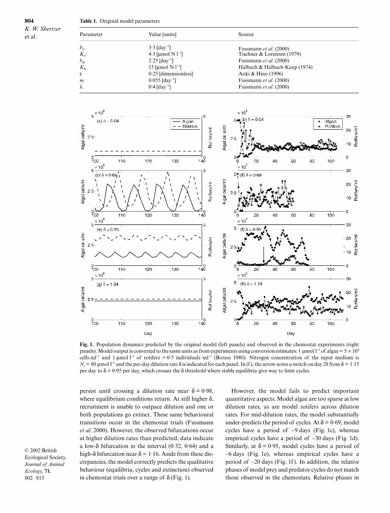
δ

(Fig. 1).

However, the model fails to predict importantquantitative aspects. Model algae are too sparse at lowdilution rates, as are model rotifers across dilutionrates. For mid-dilution rates, the model substantiallyunder-predicts the period of cycles. At

δ

= 0·69, modelcycles have a period of

∼9 days (Fig. 1c), whereasempirical cycles have a period of ∼30 days (Fig. 1d).Similarly, at δ = 0·95, model cycles have a period of∼6 days (Fig. 1e), whereas empirical cycles have aperiod of ∼20 days (Fig. 1f ). In addition, the relativephases of model prey and predator cycles do not matchthose observed in the chemostats. Relative phases in

Table 1. Original model parameters

Parameter Value [units] Source

bC 3·3 [day−1] Fussmann et al. (2000)KC 4·3 [µmol N l−1] Tischner & Lorenzen (1979)bB 2·25 [day−1] Fussmann et al. (2000)KB 15 [µmol N l−1] Halbach & Halbach-Keup (1974)ε 0·25 [dimensionless] Aoki & Hino (1996)m 0·055 [day−1] Fussmann et al. (2000)λ 0·4 [day−1] Fussmann et al. (2000)

Fig. 1. Population dynamics predicted by the original model (left panels) and observed in the chemostat experiments (rightpanels). Model output is converted to the same units as from experiments using conversion estimates: 1 µmol l−1 of algae = 5 × 104

cells ml−1 and 1 µmol l−1 of rotifers = 0·5 individuals ml−1 (Borass 1980). Nitrogen concentration of the input medium isNi = 80 µmol l−1 and the per-day dilution rate δ is indicated for each panel. In (f ), the arrow notes a switch on day 28 from δ = 1·15per day to δ = 0·95 per day, which crosses the δ threshold where stable equilibria give way to limit cycles.


805Predator–prey cycles in aquatic microcosm

© 2002 British Ecological Society, Journal of Animal Ecology, 71,802–815

the model are as expected from classical predator–preytheory in the sense that increases in rotifer density lagshortly behind increases in algal density. The observedprey and predator cycles, however, are almost exactlyout of phase so that predator maxima fall very close toprey minima.

Four hypotheses and model extensions

We extend the model of Fussmann et al. (2000) in fourdifferent ways. Each extension embodies a biologicalaspect that was excluded from the original model as atacit, simplifying assumption:1. Viability of eggs produced by rotifers increases withfood concentration.2. Nutritional value of algae increases with nitrogenavailability.3. Algal physiological state varies with the accumula-tion of toxins in the chemostat.4. Algae evolve in response to predation.It is possible that all of these aspects are present in thesystem to some degree. The question is whether any canaccount for features in the observed cycles that wentunpredicted by the original model. Source code for themodels in MATLAB is available on request from KWSor SPE.

(1)

Experimental evidence suggests that the energeticinvestment in B. calyciflorus eggs increases with foodavailability, and this investment may increase thesurvivorship of offspring (Kirk 1997). It is thereforepossible that rotifer recruitment per egg in the chemo-stats may be greater when feeding on a higher algaldensity. This concept is built into the original model byreplacing bB in equation 2b with an increasing functionof algal density, bB(C ),

eqn 3

In this function, bM is an upper bound on the maximumrotifer recruitment rate for when algal density is high.When algal density is low, bB(C ) reduces toward aproportion α1 of bM. As algal density increases, bB(C)approaches the upper bound at a rate controlled by α2.We note that bB in equation 2b was originally estimatedfrom exponentially growing rotifer populations feed-ing on high algal densities, and consequently serves asan estimate of the upper bound bM under Hypothesis 1.This leaves two new parameters, α1 and α2.

(2)

The nutritional quality of prey can affect predatorpopulation growth rates. Nutritional value of algae as a

food source for zooplankton can vary depending onalgal size (Rothhaupt 1990) and biochemical composi-tion (Ahlgren et al. 1990; Sterner 1993), both of whichcan be affected by nutrient availability. Specifically, ithas been shown that rotifer population growth ratescan be reduced when feeding on nutrient-limited algae(Rothhaupt 1995).

Again, the hypothesis is built into the original modelby replacing bB in equation 2b, this time with anincreasing function of nitrogen availability, bB(N ):

eqn 4

Here bm is the lower bound of bB(N ), realized when N iszero. The original bB in equation 2b serves as an esti-mate of the lower bound bm. It receives the oppositeinterpretation as under Hypothesis 1 because bB wasoriginally estimated from rotifer populations feedingon high algal densities with correspondingly low nitro-gen concentrations. When N is abundant in the system,bB(C ) approaches an upper bound of α3bm, whereα3 ≥ 1. The parameter α4 controls how quickly thefunction approaches its upper bound as N increases.Equation 4 tacitly assumes that the algal cell quota ofN responds instantly to the availability of N in themedium. Although not precisely correct, we justify thisassumption by observing that the time scale of algalpopulation turnover is very short relative to the periodof cycles that the model is trying to explain. The nutri-tional value model imposes two new parameters, α3

and α4.

(3)

Kirk (1998) found that unidentified autotoxins reducerotifer population growth rates and individual sur-vival. The toxic effect increases with rotifer abundance,creating a density-dependent negative feedback. In achemostat set-up, toxins accumulate if their produc-tion rate is greater than the dilution rate, as may occurduring population cycles when rotifer density is high.

The simplest toxicity model would assume a directself-limiting process: rotifer-produced toxins in themedium decrease rotifer fecundity or survival. How-ever, analysis of the original model shows that reducingthe rotifer recruitment rate would shorten the period ofcycles, not lengthen it. To give the toxins hypothesis achance of explaining the period, we posit an indirecteffect via algal quality. Rotifer population growth isassumed to diminish by feeding on toxin-contaminatedalgae, and toxin contamination also reduces the algalpopulation growth rate.

We build this hypothesis into the original model bystructuring the algal population into two classes, one‘sick’ (contaminated by toxins) and one ‘healthy’. Statevariable C1 represents the sick class and C2 representsthe healthy class so that total algal density is C1 + C2.

b C b b b eB M M MC( ) ( )( ).= + − − −α α α

1 1 1 2

b N b b b eB m m mN( ) ( )( ).= + − − −α α

3 1 4


806K. W. Shertzer et al.


The maximum recruitment rate of sick algae is aproportion α5 of that of healthy algae (i.e. bC → α5bC);maximum recruitment of healthy algae is as the ori-ginal model. Because algae are well mixed due to chem-ostat bubbling and because rotifers do not selectivelyfeed due to filter feeding, each algal class is consumedat a rate proportional to its relative density, wheretotal consumption by rotifers is FB(C1 + C2). However,rotifers are only able to convert C1 into new biomass ata fraction α6 of the rate they convert C2. The term[(α6C1 + C2)/(C1 + C2)]FB(C1 + C2) replaces the rotiferrecruitment rate FB(C ) in equations 1c and d.

It is assumed that the current rotifer abundance is anindex of the level of toxicity (this ignores lags in thewashout of toxins, possible at lower dilution rates).Additionally, it is assumed that sick algae beget onlysick algae and that healthy algae become sick throughvertical transmission. The proportion I(B) of healthyalgae producing sick algae increases with the rotiferdensity:

eqn 5

Here I(B) increases from 0 to 1 and α7 determines algalsensitivity to toxins. The toxicity model introduces oneadditional differential equation for a second algal classand three new parameters, α5, α6 and α7.

(4)

The previous hypothesis is concerned with how algalquality may vary as a consequence of rotifer density. Incontrast, Hypothesis 4 is concerned with how algalquality may vary as a selective response. The quality ofalgae as a food source can depend on edibility (Leibold1989) and digestibility (van Donk & Hessen 1993),both of which may vary with changes in morphology,structure or chemical composition. We hypothesizethat algal evolution reduces the vulnerability to preda-tion, but only at the expense of a reduction in themaximum population growth rate.

The model of Hypothesis 4 replaces FB(C) inequation 2b with FB( pC), where the function p repre-sents algal palatability relative to algae adapted to apredator-free environment. We posit an underlying algalphysiological variable z such that algal palatability andmaximum growth rate bC are functions of z. For con-venience, we let z = 0 denote the optimal trait value inthe absence of rotifers so that bC(0) = b0, where b0 takesthe value of the original maximum growth rate bC

(equation 2a). But here the constant parameter bC inequation 2a is replaced with the function bC(z):

eqn 6

This function dictates that the maximum algal growthrate decreases at a rate controlled by the parameter α8

as z departs from zero. For α8 close to 1, equation 6

describes a curve that decreases rapidly as z departsfrom 0, creating a relatively intense trade-off betweenpalatability and growth rate. Increasing α8 produces acurve that is more ‘flat’ near z = 0, which allows algaeto reduce their palatability without much cost in termsof reduced growth rate.

Because p(z) is algal palatability relative to that ofalgae adapted to a predator-free environment, p(0) = 1.As z increases, p(z) should decrease monotonically to aminimum possible value of p(z) = 0. These propertiesare met by the simple function:

eqn 7

The level of defence against predation is 1 − p(z). Theparameter α9 measures the effectiveness of the defencetrait relative to its cost. As z increases above 0, a largervalue of α9 offers greater gains in predation defencewith a smaller sacrifice in growth rate.

To describe the dynamics of z, we incorporate thestandard model for continuous-time population growththat depends on a single quantitative trait, dÇ/dt = wC,where w is the Malthusian mean fitness, or, arithmeticmean growth rate of different genotypes weighted bytheir frequencies (Crow & Kimura 1970; Lynch &Walsh 1998). We assume for simplicity that all algae ata given time have the same trait values (i.e. there is asingle genotype). An ordinary differential equationdescribes the evolution of character z (Saloniemi 1993)and is added to the system described by equations 1, 6and 7:

eqn 8

Here α10 is the additive genetic variance and ∂w/∂z is theselection gradient per unit time. The evolution modelintroduces one additional differential equation forthe underlying physiological trait and three new para-meters, α8, α9 and α10.

The original chemostat model and each of the fourextensions are implemented using a Runge–Kuttasolver with relative tolerance of 10−4. We fit the modelsto two separate data sets (from different chemostats)displaying population cycles. Both data sets are fromchemostat trials with Ni = 80 µmol l−1; one used a dilu-tion rate of δ = 0·69 per day and the other used δ = 0·95per day. Approximate replicates of the two represent-ative data sets (i.e. other data sets with Ni = 80 and δnear 0·69 or 0·95) exhibit similar dynamics in terms ofperiod, phase relationship and amplitude of predator–prey cycles. For each representative data set, we fit eachmodel in two different ways: trajectory matching and‘probe’ matching.

Trajectory matching compares model solutions withthe empirical time series. We have direct data on total

I Bee

B

B( )

.=−+

α

α

7

7

11

b z b eCz( ) , .( | | )= >−

0 88 1

α α

p ze z

( )

.=+

21 9α

˙ .zwz z C

ddt

= =

α∂∂

α∂∂10 10

1 Ç




rotifer and algal densities, and consequently matchonly the corresponding state variables (B and C, or C1

+ C2 in the case of the toxicity model). For each model,the goal is to determine values of ‘free’ parameters thatminimize the objective function E1:

eqn 9

Here BP(t) is the predicted rotifer density on day t,BO(t) is the observed rotifer density, CP(t) is the pre-dicted algal density on day t, and CO(t) is the observedalgal density. Parameters from the original chemostatmodel remain fixed at their original values (Table 1),and we search for optimal values of the new parametersin the model extensions (αi values). In addition, we treatas free parameters initial conditions for each statevariable and conversions of model units to observa-tional units (i.e. conversion of µmol l−1 to individualsml−1 for both algae and rotifers). Initial conditions needbe estimated because the data sets we analyse do notstart at ‘day 1’ of the experiments, but begin after thesystem has settled into a pattern of cycling so thatinitial values are no different from any other data point.This leaves eight or ten free parameters to be estimated,depending on the model (two or three αi values, four orfive initial conditions, and two unit conversions).

Probe matching, advocated by Kendall et al. (1999),compares models with observations based on a suite oftime series descriptors. Here the probes are chosen toaddress important features of predator–prey cycles,namely amplitude, period and phase relationship. Weuse six probes: algal maximum, algal minimum, rotifermaximum, rotifer minimum, cycle period and phasedifference. Predicted cycle features are calculated frommodel-generated time series. Observed features areestimated from the two data sets separately by ana-lysing smoothed versions of the data (see Appendixfor details). As with trajectory matching, the goal isto locate parameter values that minimize the differ-ence between prediction and observation. The probe-matching objective function E2 takes the same formas the trajectory-matching version:

eqn 10

where QP(i) is predicted value of probe i and QO(i) is thecorresponding observed probe.

However to calculate E2, initial conditions of thestate variables need not be estimated because theinterest is in long-term model behaviour, which isindependent of initial conditions. Again, originalmodel parameters remain fixed while searching foroptimal values of αi and unit conversions. This leavesfour or five free parameters to be estimated, depend-ing on the model (two or three αi values and two unitconversions).

Other possible objective functions besides E1 and E2

could be used. For example, one could maximize alikelihood function after assuming some distributionfor the errors, which in many cases yields estimatesequivalent to least squares. Objective functions couldmeasure squared error rather than absolute error or bescaled by predicted values rather than observed values.Using absolute error in E1 and E2 down-weights theeffects of outliers relative to squared error (Rousseeuw& Leroy 1987). The denominator in E1 and E2 scales theerror to be independent of measurement units, which iscritical because algal and rotifer densities may differ byup to six orders of magnitude. Scaling by observedrather than predicted values provides consistency whencomparing across the different models.

For both trajectory and probe matching, constraintsare placed on the range of possible parameter estimatesif needed to retain biological relevance. We use a two-step fitting procedure. The first step implements a geneticalgorithm to minimize the objective function (Houck,Joines & Kay 1995). Genetic algorithms are relativelyefficient optimization routines when the search space islarge, but in general are not necessarily highly accurate.The second fitting step implements a locally moreaccurate optimization routine, the Nelder–Meadsimplex algorithm, using optimal parameter valuesobtained by the genetic algorithm as initial estimates.

Results

Table 2 shows the errors obtained when fitting thevarious models to each data set using objective func-tions E1 and E2. For comparison to model fits, Table 2

Table 2. Errors E1 and E2 for optimal fits of the models and of regression splines (see Appendix). Spline errors provide a measureof baseline E1 and E2

Model

Error E1 Error E2

Data set: δ = 0·69 Data set: δ = 0·95 Data set: δ = 0·69 Data set: δ = 0·95

Spline 21·74 17·26 0·00 0·00Original 53·60 32·20 8·96 1·96Egg viab. 35·00 27·54 4·38 1·96Nutr. value 53·48 32·19 8·49 1·62Toxicity 28·83 26·91 5·54 1·47Evolution 32·41 18·83 2·60 1·39

EB t B t

B tC t C t

C tP O

O

P O

Ot1

| ( ) ( )|( )

| ( ) ( )|

( ).=

−+

−

∑

EQ i Q i

Q iP O

Oi2

1

6

| ( ) ( )|

( ),=

−

=∑




includes measures of baseline errors as calculated frompenalized regression splines (see Appendix). The originalchemostat model is a special case of each of the othermodels, and so all of the model extensions perform atleast as well as the original model. In cases that errorsof model extensions are nearly equal to those of theoriginal model, it is because optimal parameter valuesreduce the extension to approximate the original model(e.g. the nutritional value model under E1 settles onα3 ≈ 1). Table 3 shows the optimal parameter values foreach model extension.

The trajectory matches are poor (Fig. 2). The eggviability and nutritional value models utterly fail toreplicate the dynamic behaviour in the data. Thetoxicity model at δ = 0·69 is at least able to predictrotifer cycles with approximately the correct period,but at the expense of mismatching the period of corre-sponding algal cycles. At the higher dilution rate, thetoxicity model is unable to reproduce the observeddynamics. In general, the evolution model outperformsthe other models. It predicts rotifer cycles with approx-imately the correct period in each data set and adequately

Table 3. Optimal parameter values. Each model extension also contains all parameters from the original model, held fixed duringoptimization

Parameter (model)

Error E1 Error E2

Data set: δ = 0·69 Data set: δ = 0·95 Data set: δ = 0·69 Data set: δ = 0·95

α1 (Egg viab.) 0·13 0·91 0·02 0·55α2 (Egg viab.) 0·06 0·003 0·21 14·86α3 (Nutr. value) 1·01 1·00 2·12 1·01α4 (Nutr. value) 1·06 0·14 14·50 13·31α5 (Toxicity) 0·34 0·68 0·99 0·56α6 (Toxicity) 0·70 0·90 0·88 0·9α7 (Toxicity) 3·07 2·14 42·57 8·49α8 (Evolution) 1·25 1·17 1·41 1·58α9 (Evolution) 6·24 5·28 9·93 8·45α10 (Evolution) 0·10 0·13 0·06 0·15

Fig. 2. Optimal model fits to observed chemostat data using objective function E1. (a) Algae at δ = 0·69. (b) Rotifers at δ = 0·69.(c) Algae at δ = 0·95. (d) Rotifers at δ = 0·95.




describes the correct predator–prey phase relationships.However, it does not capture algal peaks well, especiallyat δ = 0·69 per day.

In probe matching, the evolution model again out-performs the other models (Table 2). Table 4 displaysthe cycle features estimated from data and predicted byoptimal model fits. The egg viability model cannotincrease the period beyond what is predicted by theoriginal model. The nutritional value model and thetoxicity model can potentially approximate the observedperiod, but only at the expense of an increase in thephase-relationship error term. Because of this trade-offbetween the two error terms, ultimately neither modelmatches the period adequately. The evolution modelbest matches the observed period without a consequen-tial increase in the error due to mismatching the phaserelationship.

In both trajectory and probe matching, parametersare estimated separately at each dilution rate. Despiteefforts to maintain consistent conditions across replic-ates, chemostats with nominally identical parameterscan exhibit different dynamics (Fussmann et al. 2000),so it would not have been sensible to try fitting bothdata sets by a single set of parameters in each model.Nevertheless, a good mechanistic model should havestable estimates across data sets and across fitting cri-teria. The evolution model has the most stable para-meter estimates (Table 3), as measured by the averagepercentage difference between estimates for the twodata sets or error functions. Because the evolutionmodel performs best in terms of cycle matching andparameter stability, we further examine the data for anycorroborative evidence of algal evolution.

Built into the evolution model is a trade-off betweenalgal growth and resistance to predation. When rotiferdensity is low, selection for high algal growth leads to

relatively low defence and high algal palatability.Increased palatability leads to higher rotifer recruit-ment per captured prey. This departs from the standardassumption that the functional response depends onlyon organism quantities. Instead, the evolution modelpredicts that, for any given algal density, per-capitarotifer recruitment rates are higher following lowrotifer densities than following high rotifer densitiesbecause that is when selection promotes increased algalpalatability. Here we examine whether data from thechemostat experiments support that prediction.

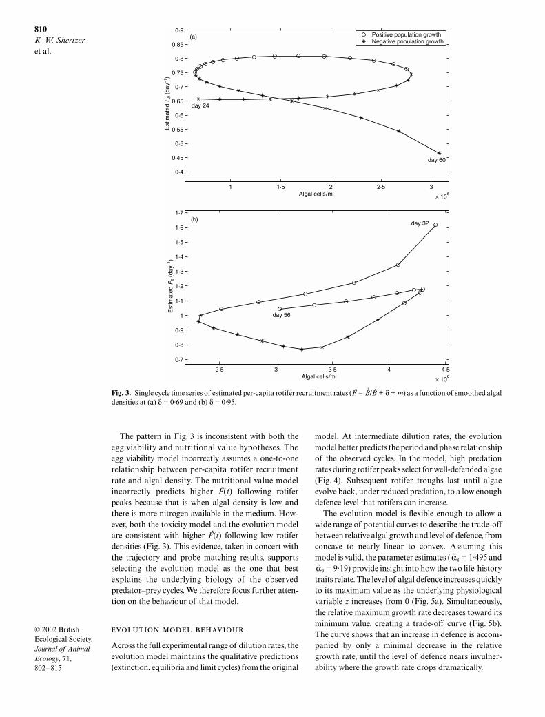
It follows from equation 1d that total rotiferrecruitment is B + (δ + m)B, so per-capita recruitmentis FB = B/B + δ + m. To estimate FB, we first estimatea continuous version of B(t) by fitting a regressionspline to the empirical time series of rotifer densities(Fig. A1a,b), and then estimate B(t) as the derivative ofthat spline (Fig. A1e,f ). We also estimate a continuousversion of algal densities C(t) by fitting a regressionspline (Fig. A1a,b). Figure 3 plots the estimatedtime series of per-capita rotifer recruitment rates F(t)against smoothed algal densities over a cycle from eachdata set.

If FB(t) depended solely on algal density, then Fig. 3would illustrate a one-to-one correspondence. Instead,it displays a pattern of multiple per-capita rotiferrecruitment rates for any given algal density, withhigher recruitment rates following low rotifer densitiesas predicted by the evolution model. Similar analysesof cycles from other data sets show the same pattern(not plotted here), and so unless there is some unlikelysystematic bias in sampling, the pattern is not due tomeasurement error. The pattern is potentially due toshifts in the age structure accompanied by decay inrotifer fecundity, but this is unlikely at high dilutionrates where rotifers wash out of the system before theyhave a chance to senesce. In fact, the effects of agestructure simulated by the original model at δ = 0·95are much smaller than in Fig. 3.

Table 4. Descriptive features of cycles (probes) estimated from data (QO) and predicted by optimal model fits (QP). Features are:(1) = algal minimum (cells ml−1); (2) = algal maximum (cells ml−1); (3) = rotifer minimum (rotifers ml−1); (4) = rotifer maximum(rotifers ml−1); (5) = cycle period (days); (6) = phase-relationship (days)

Feature QO QP Original QP Egg viab. QP Nutr. value QP Toxicity QP Evolution

δδδδ ==== 0·69(1) 663 400 54 264 663 400 0·01 663 400 1310 800(2) 2974 600 2974 600 2974 600 3147 300 697 500 1566 000(3) 6·66 1·7 6·75 0·002 6·7 0·39(4) 14·65 14·65 12·51 28·85 6·81 14·65(5) 30·93 9·3 5·4 16·5 5·3 30·6(6) 0·25 1·9 1·1 1·5 1·1 0·3

δδδδ ==== 0·95(1) 2045 500 2045 500 2045 500 203 780 1834 200 2045 500(2) 4689 500 3534 600 3534 600 476 010 4782 500 2274 200(3) 1·34 1·34 1·34 1·34 1·34 1·34(4) 5·87 1·67 1·67 1·92 2·95 5·87(5) 20·5 5·7 5·7 6·1 12·5 20·1(6) 2·06 1·5 1·5 1·6 3·0 0·3

JAE_645.fm 09 Monday, August 26, 2002 10:17 AM



The pattern in Fig. 3 is inconsistent with both theegg viability and nutritional value hypotheses. Theegg viability model incorrectly assumes a one-to-onerelationship between per-capita rotifer recruitmentrate and algal density. The nutritional value modelincorrectly predicts higher F(t) following rotiferpeaks because that is when algal density is low andthere is more nitrogen available in the medium. How-ever, both the toxicity model and the evolution modelare consistent with higher F(t) following low rotiferdensities (Fig. 3). This evidence, taken in concert withthe trajectory and probe matching results, supportsselecting the evolution model as the one that bestexplains the underlying biology of the observedpredator–prey cycles. We therefore focus further atten-tion on the behaviour of that model.

Across the full experimental range of dilution rates, theevolution model maintains the qualitative predictions(extinction, equilibria and limit cycles) from the original

model. At intermediate dilution rates, the evolutionmodel better predicts the period and phase relationshipof the observed cycles. In the model, high predationrates during rotifer peaks select for well-defended algae(Fig. 4). Subsequent rotifer troughs last until algaeevolve back, under reduced predation, to a low enoughdefence level that rotifers can increase.

The evolution model is flexible enough to allow awide range of potential curves to describe the trade-offbetween relative algal growth and level of defence, fromconcave to nearly linear to convex. Assuming thismodel is valid, the parameter estimates ( 8 = 1·495 and

9 = 9·19) provide insight into how the two life-historytraits relate. The level of algal defence increases quicklyto its maximum value as the underlying physiologicalvariable z increases from 0 (Fig. 5a). Simultaneously,the relative maximum growth rate decreases toward itsminimum value, creating a trade-off curve (Fig. 5b).The curve shows that an increase in defence is accom-panied by only a minimal decrease in the relativegrowth rate, until the level of defence nears invulner-ability where the growth rate drops dramatically.

Fig. 3. Single cycle time series of estimated per-capita rotifer recruitment rates (F = ı/∫ + δ + m) as a function of smoothed algaldensities at (a) δ = 0·69 and (b) δ = 0·95.

α̂α̂




Discussion

The chemostat model of Fussmann et al. (2000)accurately predicted the qualitative dynamics observedin an experimental community over a range of environ-mental conditions. The fundamental issue of thispaper is to identify a plausible biological mechanismto account for features in the predator–prey cyclesincorrectly predicted by the original model, particularlythe observed period and phase relationship (rotifermaxima coinciding with algal minima). Of the fourmodels built to identify that mechanism, three areinconsistent with the chemostat data. The egg viabilitymodel cannot generate the longer period cycles. Thenutritional value model and the toxicity model canpotentially generate longer cycles, but then mismatchthe observed phase relationship. Only the evolutionmodel is able to match the correct period and phaserelationship simultaneously. In addition, it bestmatches the chemostat data (Table 2) and has the moststable parameter estimates across data sets and fittingcriteria (Table 3).

During predator–prey cycles, the observed per-capita rotifer recruitment rates (Fig. 3) are compatiblewith the evolution model in three ways. First, there isnot a one-to-one relationship between algal densitiesand per-capita rotifer recruitment rates, explained inthe model by variation in algal palatability. In general,this could also be explained by predator interference inthe functional response (review in Skalski & Gilliam2001), but this is unlikely here because the phase rela-tionship in the experimental cycles is such that there aremany pairs of times when algal and rotifer densities areboth nearly equal [C(t1) = C(t2), B(t1) = B(t2)] while therotifer growth rate is highly positive at one time andhighly negative at the other. Second, per-capita rotiferrecruitment rates at a given algal density are lowerwhen the rotifer population is decreasing than when itis increasing, which occurs in the model due to evolu-tion of well-defended algae during high rotifer densities.Third, the model predicts that palatability is highest inthe middle of the rotifers’ increasing phase, and lowestin the middle of the rotifers’ decreasing phase (Fig. 4).This is consistent with the timing of the greatest

Fig. 4. Behaviour of evolution model at (a) δ = 0·69 and (b) δ = 0·95. Algal defence is 1 − p, where p is relativepalatability. Parameter values ( 8 = 1·495, 9 = 9·19, 10 = 0·105) are the average estimates from probe matching across the twodata sets.

α̂ α̂ α̂




difference in observed per-capita rotifer recruitmentrates for a given algal density (Fig. 3).

The evolution model, although better able to matchthe data than the others, still provides an unsatisfyingfit in absolute terms. In particular, the model under-predicts the amplitude of algal cycles in both trajectoryand probe matching. This indicates that there are twodistinct pieces missing from the original chemostat model:one to explain the period and phase-relationship andone to explain the amplitude of algal cycles. We believethis study has resolved the first, and the second remainsunidentified, although aspects of the rotifer functionalor numerical responses are good candidates. Trajectorymatching is a lot to ask from an incompletely specifiedmechanistic model, and the lack of fit there in partmotivated the use of probe matching to reveal under-lying mechanisms.

In the evolution model, evolutionary dynamics havea destabilizing effect over a wide range of dilution rates.Cycles are generated by an evolutionary trade-offbetween high algal growth rates and defence againstpredation. As rotifer density rises, selection for

increased algal defence drives down palatability untilrotifer density declines. The subsequent rotifer troughlasts until algae evolve back to a low enough defencelevel that rotifers can again increase. This response toselection accrues over multiple generations, unlike theresponse of phenotypic plasticity. Without the evolu-tionary lag, the longer cycles would not be explained.

Other investigations have considered the effects ofprey evolution on the stability of prey and predatordynamics (review in Abrams 2000). There is no generalconsensus; prey evolution can be either stabilizing ordestabilizing (Abrams 2000). In destabilizing cases,Abrams & Matsuda (1997) note the possibility of apositive feedback between cycle amplitude and relaxedselection on prey defence. Thus, prey evolution canproduce diverging oscillations. Here evolution doesnot produce diverging oscillations, and can result inincreased or decreased amplitude of population cyclesdepending on the dilution rate. Instead, our modeldemonstrates that prey evolution can substantiallyincrease the period of predator–prey cycles and canaffect the phase relationship between them.

Fig. 5. (a) Algal population growth rate (bC) and predation defence (1 − p) as functions of the underlying physiological variablez. (b) The resulting trade-off curve between the two life-history traits.




The model system here provides a unique opportunityto explore how evolution and population dynamicsinterrelate, which is difficult to study outside the labo-ratory because of the need for long-term populationdata. Experiments are now in progress to test theevolution hypothesis directly. One component has beensupported: rotifer population growth rates are reducedwhen feeding on algae cultivated under grazing pres-sure, relative to algae cultivated under comparablemortality rates due to an elevated washout rate (T.Yoshida, S. Ellner & N. Hairston, Jr, unpublisheddata). The nature of the hypothesized physiologicaltrait z is not yet known. Plausible candidates includecell size, durability of cell walls and defensive toxins.Larger cell size may offer a refuge from predation;harder/thicker cell walls may allow algae to passthrough rotifer guts unharmed; and defensive toxinproduction may be stimulated by the presence ofpredators. Experiments to test for changes in thesetraits in response to predation, and for correlatedchanges in algal population growth rate, are currentlybeing designed.

In summary, we find little evidence to support threeof the four hypotheses meant to explain observedfeatures in the rotifer–algal cycles. Only the model thatincludes evolutionary dynamics of prey can reproducethe observed period and phase relationship simultane-ously, and is supported by corroborative evidence.While still very simple, the evolution model greatlyimproves predictions for the chemostat system andoffers insights into how prey evolution can affectpredator–prey dynamics.

Acknowledgements

We thank Jim Gilliam, James Grover, Ken Pollock,Len Stefanski and an anonymous referee for helpfulcomments on the manuscript. Support was providedby a grant from the Andrew Mellon Foundation toS.P.E. and N.G.H. Jr.

References

Abrams, P.A. (2000) The evolution of predator–prey interac-tions: theory and evidence. Annual Review of Ecology andSystematics, 31, 79–105.

Abrams, P.A. & Matsuda, H. (1997) Prey evolution as a causeof predator–prey cycles. Evolution, 51, 1740–1748.

Ahlgren, G., Lundstedt, L., Brett, M. & Forsberg, C. (1990)Lipid composition and food quality of some freshwaterphytoplankton for cladoceran zooplankters. Journal ofPlankton Research, 12, 809–818.

Aoki, S. & Hino, A. (1996) Nitrogen flow in a chemostatculture of the rotifer Brachionus plicatilis. Fisheries Science,62, 8–14.

Berryman, A.A. (1992) The origins and evolution of predatory–prey theory. Ecology, 73, 1530–1535.

Borass, M.E. (1980) A chemostat system for the study ofrotifer–algal–nitrate interactions. American Society ofLimnology and Oceanography Special Symposium, 3, 173–182.

Carpenter, S.R., Cottingham, K.L. & Stow, C.A. (1994)Fitting predator–prey models to time series with observa-tion errors. Ecology, 75, 1254–1264.

Costantino, R.F., Desharnais, R.A., Cushing, J.M. & Dennis, B.(1997) Chaotic dynamics in an insect population. Science,275, 389–391.

Crow, J.F. & Kimura, M. (1970) An Introduction to PopulationGenetics Theory. Harper & Row, New York.

van Donk, E. & Hessen, D.O. (1993) Grazing resistance innutrient-stressed phytoplankton. Oecologia, 93, 508–511.

Ellner, S.P. & Seifu, Y. (2002) Using spatial statistics to selectmodel complexity. Journal of Computational and GraphicalStatistics, 11, 348–369.

Ellner, S.P., McCauley, E., Kendall, B.E., Briggs, C.J.,Hosseini, P.R., Wood, S.N., Janssen, A., Sabelis, M.W.,Turchin, P., Nisbet, R.M. & Murdoch, W.W. (2001) Habitatstructure and population persistence in an experimentalcommunity. Nature, 412, 538–542.

Fussmann, G.F., Ellner, S.P., Shertzer, K.W. & Hairston, N.G. Jr(2000) Crossing the Hopf bifurcation in a live predator–prey system. Science, 290, 1358–1360.

Green, P.J. & Silverman, B.W. (1994) Nonparametric Regres-sion and Generalized Linear Models: a Roughness PenaltyApproach. Chapman & Hall, London.

Halbach, U. & Halbach-Keup, G. (1974) Quantitative Bezie-hungen zwischen Phytoplankton und der Populationsdy-namik des Rotators Brachionus calyciflorus Pallas. Befundeaus Laboratoriumsexperimenten und Freilanduntersuc-hungen. Archiv fur Hydrobiologie, 73, 273–309.

Harrison, G.W. (1994) Comparing predator–prey models toLuckinbill’s experiment with Didinium and Paramecium.Ecology, 76, 357–374.

Holling, C.S. (1959) Some characteristics of simple types ofpredation and parasitism. Canadian Entemologist, 91, 385–395.

Houck, C.R., Joines, J.A. & Kay, M.G. (1995) A GeneticAlgorithm for Function Optimization: a MATLAB Imple-mentation. Technical Report 9509, Department ofIndustrial Engineering, North Carolina State University.Raleigh, USA.

Kendall, B.E., Briggs, C.J., Murdoch, W.W., Turchin, P.,Ellner, S.P., McCauley, E., Nisbet, R.M. & Wood, S.N.(1999) Why do populations cycle? A synthesis of statisticaland mechanistic modeling approaches. Ecology, 80, 1789–1805.

Kirk, K.L. (1997) Egg size, offspring quality and food level inplanktonic rotifers. Freshwater Biology, 37, 515–521.

Kirk, K.L. (1998) Enrichment can stabilize populationdynamics: autotoxins and density dependence. Ecology, 79,2456–2462.

Leibold, M.A. (1989) Resource edibility and the effect ofpredators and productivity on the outcome of trophic inter-actions. American Naturalist, 134, 922–949.

Lynch, M. & Walsh, J.B. (1998) Genetics and Analysis ofQuantitative Traits. Sinauer Associates, Inc, Sunderland,MA.

Monod, J. (1950) La technique de culture continue; theorie etapplications. Annals de l’Institut Pasteur, 79, 390–410.

Nelson, W.A., McCauley, E. & Wrona, F.J. (2001) Multipledynamics in a single predator-prey system: experimentaleffects of food quality. Proceedings of the Royal SocietyLondon B, 268, 1223–1230.

Rothhaupt, K.O. (1990) Population growth rates of twoclosely related rotifer species: effects of food quantity,particle size, and nutritional quality. Freshwater Biology,23, 561–570.

Rothhaupt, K.O. (1995) Algal nutrient limitation affectsrotifer growth rate but not ingestion rate. Limnology andOceanography, 40, 1201–1208.




Rousseeuw, P.J. & Leroy, A.M. (1987) Robust Regression andOutlier Detection. John Wiley and Sons, New York.

Saloniemi, I. (1993) A coevolutionary predator–prey modelwith quantitative characters. American Naturalist, 141,880–896.

Simonoff, J.S. (1996) Smoothing Methods in Statistics.Springer Series in Statistics. Springer-Verlag, New York.

Skalski, G.T. & Gilliam, J.F. (2001) Functional responses withpredator interference: viable alternatives to the HollingType II model. Ecology, 82, 3083–3092.

Sterner, R.W. (1993) Daphnia growth on varying quality ofScenedesmus: mineral limitation of zooplankton. Ecology,74, 2351–2360.

Strogatz, S.H. (1994) Nonlinear Dynamics and Chaos. Addison-Wesley, Reading, MD.

Tischner, R. & Lorenzen, H. (1979) Nitrate uptake andnitrate reduction in synchronous Chlorella. Planta, 146,287–292.

Received 18 December 2001; revision received 10 May 2002

Appendix

We use penalized regression splines to obtain smooth,continuous versions of the data and estimate gradientsof population trajectories. Penalized regression splinesare detailed elsewhere (Green & Silverman 1994;Simonoff 1996); here we focus on a key aspect thatdetermines the amount of fidelity to data: the smooth-ing parameter.

We consider two different objective methods forselecting the smoothing parameter: residual spatialautocorrelation (RSA) and cross-validation (CV).RSA is based on spatial autocorrelation of residualsfrom the fitted model (Ellner & Seifu 2002). An insuf-ficiently complex model is unable to fit structure in thedata, and consequently the residuals exhibit positiveautocorrelation in the space of the independent varia-ble. The selection criterion is to adjust the smoothing

parameter until a Moran’s I statistic (a measure ofresidual spatial autocorrelation) equals to zero.

Residual spatial autocorrelation tends to be conserv-ative in selecting model complexity (Ellner & Seifu 2002).The fits therefore do not display spurious wiggles, butthis potentially comes at the expense of underfittingextrema. To check the validity of fits from RSA, wecompare them to fits from CV, a less conservativemethod. Here the goal of CV is to choose the smooth-ing parameter so as to minimize the leave-one-outcross-validation score (Simonoff 1996).

RSA fits to empirical cycles are very smooth(Fig. A1a,b). Because CV fits have less of a tendencyto underfit extrema, we use those splines (Fig. A1c,d)to estimate maxima and minima of algal and rotiferdensities. However, these values are reassuringly verysimilar to the corresponding estimates produced bythe RSA splines. To estimate the period and phase

Fig. A1. Smoothed population densities and gradients of rotifers (- -) and algae (—) plotted alongside rotifer data (�) and algaldata (�). (a) RSA regression splines for data set δ = 0·69. (b) RSA regression splines for data set δ = 0·95. (c) CV regression splinesfor data set δ = 0·69 and (d) CV regression splines for data set δ = 0·95. (e) Gradients of the RSA splines for data set δ = 0·69.(f) Gradients of the RSA splines for data set δ = 0·95.




relationship, we use gradients of the RSA fits (Fig. A1e,f).The gradients cross zero at points in time correspond-ing to when the estimated population trajectories reachmaxima or minima. The timing of these peaks providesan estimate of the period (twice the duration of maximumto minimum) for each data set. As a measure of thephase difference for each data set, we calculate the aver-age distance between locations of rotifer maxima and

algal minima and locations of rotifer minima and algalmaxima. This is actually the phase difference minushalf the period, which is accounted for when probematching.

In Table 2, baseline errors for E1 are calculated fromRSA fits. Baseline errors for E2 are zero because it is theregression splines that are used to calculate observedcycle features Q0 against which each model is measured.


jae 645.fm page 802 monday, august 26, 2002 10:17 am...

Documents