james k. peterson - clemson university
TRANSCRIPT

MATH 4530: Analysis One
Limits and Continuity in <2 and <3
James K. Peterson
Department of Biological Sciences and Department of Mathematical SciencesClemson University
April 10, 2019

MATH 4530: Analysis One
Outline
1 <2 and <3
2 Functions of Two Variables
3 Continuity
MATH 4530: Analysis One
<2 and <3
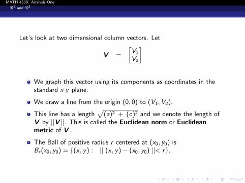
Let’s look at two dimensional column vectors. Let
V =
[V1
V2
]
We graph this vector using its components as coordinates in thestandard x y plane.
We draw a line from the origin (0, 0) to (V1,V2).
This line has a length√
(a)2 + (c)2 and we denote the length ofV by ||V ||. This is called the Euclidean norm or Euclideanmetric of V .
The Ball of positive radius r centered at (x0, y0) isBr (x0, y0) = {(x , y) : || (x , y)− (x0, y0) ||< r}.

MATH 4530: Analysis One
<2 and <3
V
V1
V2
x
y
||V ||
A vector V can be iden-tified with an order pair(V1,V2). The components(V1,V2) are graphed in theusual Cartesian manner asan ordered pair in plane.The magnitude of V is|| V ||.
MATH 4530: Analysis One
<2 and <3
Let V and W be column vectors of size 2× 1:
V =
[V1
V2
], W =
[W1
W2
].
We define their inner product to be the real number
< V , W > = V1W1 + V2W2.
This is also denoted by V · W .

MATH 4530: Analysis One
<2 and <3
Let’s look at three dimensional column vectors. Let
V =
V1
V2
V3
We graph this vector using its components as coordinates in thestandard x y z coordinate system.
We draw a line from the origin (0, 0, 0) to (V1,V2,V3).
This line has a length√
(V1)2 + (V2)2 + (V3)2 and we denote thelength of V by ||V ||. This is also called the Euclidean norm orEuclidean metric of V . We can usually tell which norm we need ascontext tells us if we are in two or three dimensional situation.
The Ball of positive radius r centered at (x0, y0, z0) isBr (x0, y0, z0) = {(x , y , z) : || (x , y , z)− (x0, y0, z0) ||< r}.

MATH 4530: Analysis One
<2 and <3
Let V and W be column vectors of size 3× 1:
V =
V1
V2
V3
, W =
W1
W2
W3
.We define their inner product to be the real number
< V , W > = V1W1 + V2W2 + V3W3
This is also denoted by V · W .
MATH 4530: Analysis One
Functions of Two Variables
Now let’s start looking at functions that map each ordered pair(x , y) into a number. Let’s begin with an example. Consider thefunction f (x , y) = x2 + y2 defined for all x and y .
Hence, for each x and y we pick, we calculate a number we candenote by z whose value is f (x , y) = x2 + y2. Using the same ideaswe just used for the x − y plane, we see the set of all such triples(x , y , z) = (x , y , x2 + y2) defines a surface in <3 which is thecollection of all ordered triples (x , y , z).
We can plot this surface in MatLab with fairly simple code. Let’s gothrough how to do these plots in a lot of detail so we can see howto apply this kind of code in other situations.
To draw a portion of a surface, we pick a rectangle of x and yvalues. To make it simple, we will choose a point (x0, y0) as thecenter of our rectangle and then for a chosen ∆x and ∆y andintegers nx and ny , we set up the rectangle
[x0 − nx∆x , . . . , x0, . . . , x0 + nx∆x ]
× [y0 − ny∆y , . . . , y0, . . . , y0 + ny∆y ]

MATH 4530: Analysis One
Functions of Two Variables
The constant x and y lines determined by this grid result in a matrixof intersections with entries (xi , yj) for appropriate indices i and j .
We will approximate the surface by plotting the triples(xi , yj , zij = f (xi , yj)) and then drawing a top for each rectangle.
Right now though, let’s just draw this base grid. In MatLab, firstsetup the function we want to look at. We will choose a very simpleone
f = @( x , y ) x . ˆ2 + y . ˆ 2 ;
MATH 4530: Analysis One
Functions of Two Variables
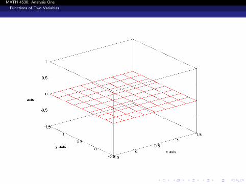
Now, we draw the grid by using the functionDrawGrid(f,delx,nx,dely,ny,x0,y0). This function has severalarguments as you can see and we explain them in the listing below. Sowe are drawing a grid centered around (0.5, 0.5) using a uniform 0.5 stepin both directions. The grid is drawn at z = 0.
% Taking the arguments i n o r d e r% f i s the s u r f a c e f u n c t i o n% de l x = 0 .5 i s the width o f the d e l t a x% nx = 2 i s the number o f s t e p s we take r i g h t and l e f t from% the base po i n t x0% de l y = 0 .5 i s the width o f the d e l t a y% ny = 2 i s the number o f s t e p s we take r i g h t and l e f t from% the base po i n t y0% x0 = 0 .5% y0 = 0 .5DrawGrid ( f , 0 . 5 , 2 , 0 . 5 , 2 , 0 . 5 , 0 . 5 ) ;
MATH 4530: Analysis One
Functions of Two Variables
MATH 4530: Analysis One
Functions of Two Variables
Make sure you play with the plot a bit. You can grab it and rotateit as you see fit to make sure you see all the detail. Right now, thereis not much to see in the grid, but later when we plot the surface,the grid and other things, the ability to rotate in 3D is important toour understanding. So make sure you take the time to see how todo this!
To draw the surface, we find the pairs (xi , yj) and the associatedf (xi , yj) values and then call theDrawMesh(f,delx,nx,dely,ny,x0,y0) command. The meaningin the arguments is the same as in DrawGrid so we won’t repeatthem here.
DrawMesh ( f , 0 . 5 , 2 , 0 . 5 , 2 , 0 . 5 , 0 . 5 ) ;

MATH 4530: Analysis One
Functions of Two Variables
The resulting surface and grid is shown here.
MATH 4530: Analysis One
Functions of Two Variables
Next, we draw the traces corresponding to the values x0 and y0.The x0 trace is the function f (x0, y) which is a function of the twovariables y and z . The y0 trace is the function f (x , y0) which is afunction of the two variables x and z . We plot these curves usingthe function DrawTraces.
DrawTraces ( f , 0 . 5 , 2 , 0 . 5 , 2 , 0 . 5 , 0 . 5 ) ;

MATH 4530: Analysis One
Functions of Two Variables
The resulting surface with grid and traces is shown here. Thetraces are the thick parabolas on the surface.
MATH 4530: Analysis One
Functions of Two Variables
Next, let’s add the column with the rectangular base havingcoordinates Lower Left (x0, y0), Lower Right (x0 + ∆x , y0), UpperLeft (x0, y0 + ∆y) and Upper Right (x0 + ∆x , y0 + ∆y).
We draw and fill this base with the function DrawBase. We drawthe vertical lines going from each of the four corners of the base tothe surface with the code DrawColumn and we draw and fill thepatch of surface this column creates in the full surface with thefunction DrawPatch.
MATH 4530: Analysis One
Functions of Two Variables
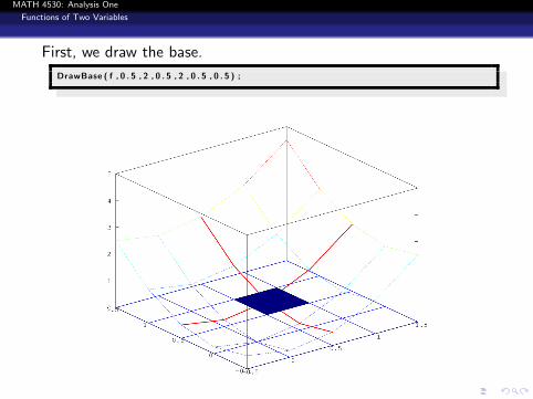
First, we draw the base.
DrawBase ( f , 0 . 5 , 2 , 0 . 5 , 2 , 0 . 5 , 0 . 5 ) ;
MATH 4530: Analysis One
Functions of Two Variables
In DrawColumn, we draw four vertical lines from the base up to thesurface. You’ll note the figure is getting more crowded lookingthough. Make sure you grab the picture and rotate it around so youcan see everything from different perspectives.
DrawColumn ( f , 0 . 5 , 2 , 0 . 5 , 2 , 0 . 5 , 0 . 5 ) ;
We then draw the patch just like we drew the base.
DrawPatch ( f , 0 . 5 , 2 , 0 . 5 , 2 , 0 . 5 , 0 . 5 ) ;
The resulting surface with grid and traces and with the column andpatch is shown in the next figure.

MATH 4530: Analysis One
Functions of Two Variables

MATH 4530: Analysis One
Functions of Two Variables
We have combined all of these functions into a utility functionDrawSimpleSurface which manages these different graphingchoices using boolean variables like DoGrid to turn a graph on oroff.
If the boolean variable DoGrid is set to one, the grid is drawn. Thecode is self-explanatory so we just lay it out here.
We haven’t shown all the code for the individual drawing functions,but we think you’ll find it interesting to see how we manage thepieces in this one piece of code. So check this out.

MATH 4530: Analysis One
Functions of Two Variables
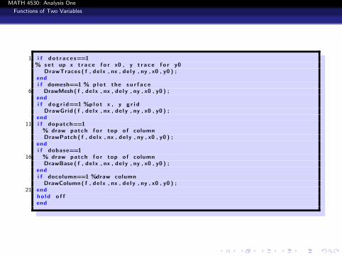
First, let’s explain the arguments
f u n c t i o n DrawSimpleSur face ( f , de l x , nx , de l y , ny , x0 , y0 , domesh , do t r ace s , dog r i d ,dopatch , docolumn , dobase )
% f i s the f u n c t i o n d e f i n i n g the s u r f a c e% de l x i s the s i z e o f the x s t ep% nx i s the number o f s t e p s l e f t and r i g h t from x0
5 % de l y i s the s i z e o f the y s t ep% ny i s the number o f s t e p s l e f t and r i g h t from y0% ( x0 , y0 ) i s the l o c a t i o n o f the column r e c t a n g l e base% domesh = 1 means do the mesh , d og r i d = 1 imeans do the g r i d% dopatch = 1 means add the patch above the column
10 % dobase = 1 means add the base o f the column% docolumn = 1 add the column , d o t r a c e s = 1 add the t r a c e s%% s t a r t ho ldho ld on
Now look at the code
MATH 4530: Analysis One
Functions of Two Variables
1 i f d o t r a c e s==1% se t up x t r a c e f o r x0 , y t r a c e f o r y0
DrawTraces ( f , de l x , nx , de l y , ny , x0 , y0 ) ;endi f domesh==1 % p l o t the s u r f a c e
6 DrawMesh ( f , de l x , nx , de l y , ny , x0 , y0 ) ;endi f d og r i d==1 %p l o t x , y g r i d
DrawGrid ( f , de l x , nx , de l y , ny , x0 , y0 ) ;end
11 i f dopatch==1% draw patch f o r top o f columnDrawPatch ( f , de l x , nx , de l y , ny , x0 , y0 ) ;
endi f dobase==1
16 % draw patch f o r top o f columnDrawBase ( f , de l x , nx , de l y , ny , x0 , y0 ) ;
endi f docolumn==1 %draw column
DrawColumn ( f , de l x , nx , de l y , ny , x0 , y0 ) ;21 end
ho ld o f fend
MATH 4530: Analysis One
Functions of Two Variables
Hence, to draw everything for this surface, we would use the session:
>> f = @( x , y ) x .ˆ2+y . ˆ 2 ;>> DrawSimpleSur face ( f , 0 . 5 , 2 , 0 . 5 , 2 , 0 . 5 , 0 . 5 , 1 , 1 , 1 , 1 , 1 , 1 ) ;
This surface has circular cross sections for different positive values of z
and it is called a circular paraboloid. If you used f (x , y) = 4x2 + 3y2, the
cross sections for positive z would be ellipses and we would call the
surface an elliptical paraboloid. Now this code is not perfect. However,
as an exploratory tool it is not bad! Now it is time for you to play with it
a bit in the exercises below.

MATH 4530: Analysis One
Continuity
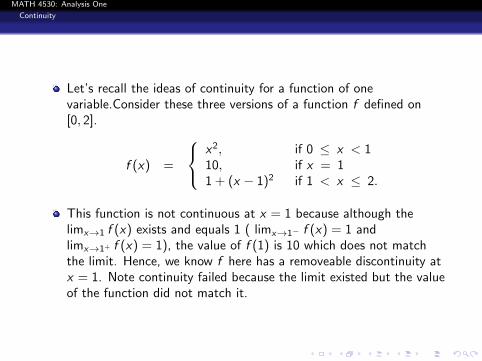
Let’s recall the ideas of continuity for a function of onevariable.Consider these three versions of a function f defined on[0, 2].
f (x) =
x2, if 0 ≤ x < 110, if x = 11 + (x − 1)2 if 1 < x ≤ 2.
This function is not continuous at x = 1 because although thelimx→1 f (x) exists and equals 1 ( limx→1− f (x) = 1 andlimx→1+ f (x) = 1), the value of f (1) is 10 which does not matchthe limit. Hence, we know f here has a removeable discontinuity atx = 1. Note continuity failed because the limit existed but the valueof the function did not match it.
MATH 4530: Analysis One
Continuity
Let’s recall the ideas of continuity for a function of onevariable.Consider these three versions of a function f defined on[0, 2].
f (x) =
x2, if 0 ≤ x < 110, if x = 11 + (x − 1)2 if 1 < x ≤ 2.
This function is not continuous at x = 1 because although thelimx→1 f (x) exists and equals 1 ( limx→1− f (x) = 1 andlimx→1+ f (x) = 1), the value of f (1) is 10 which does not matchthe limit. Hence, we know f here has a removeable discontinuity atx = 1. Note continuity failed because the limit existed but the valueof the function did not match it.

MATH 4530: Analysis One
Continuity
The second version of f is given below.
f (x) =
{x2, if 0 ≤ x ≤ 1(x − 1)2 if 1 < x ≤ 2.
In this case, the limx→1− = 1 and f (1) = 1, so f is continuous fromthe left. However, limx→1+ = 0 which does not match f (1) and so fis not continuous from the right. Also, since the right and left handlimits do not match at x = 1, we know limx→1 does not exist. Here,the function fails to be continuous because the limit does not exist.
MATH 4530: Analysis One
Continuity
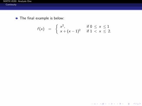
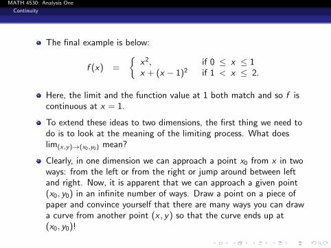
The final example is below:
f (x) =
{x2, if 0 ≤ x ≤ 1x + (x − 1)2 if 1 < x ≤ 2.
Here, the limit and the function value at 1 both match and so f iscontinuous at x = 1.
To extend these ideas to two dimensions, the first thing we need todo is to look at the meaning of the limiting process. What doeslim(x,y)→(x0,y0) mean?
Clearly, in one dimension we can approach a point x0 from x in twoways: from the left or from the right or jump around between leftand right. Now, it is apparent that we can approach a given point(x0, y0) in an infinite number of ways. Draw a point on a piece ofpaper and convince yourself that there are many ways you can drawa curve from another point (x , y) so that the curve ends up at(x0, y0)!

MATH 4530: Analysis One
Continuity
The final example is below:
f (x) =
{x2, if 0 ≤ x ≤ 1x + (x − 1)2 if 1 < x ≤ 2.
Here, the limit and the function value at 1 both match and so f iscontinuous at x = 1.
To extend these ideas to two dimensions, the first thing we need todo is to look at the meaning of the limiting process. What doeslim(x,y)→(x0,y0) mean?
Clearly, in one dimension we can approach a point x0 from x in twoways: from the left or from the right or jump around between leftand right. Now, it is apparent that we can approach a given point(x0, y0) in an infinite number of ways. Draw a point on a piece ofpaper and convince yourself that there are many ways you can drawa curve from another point (x , y) so that the curve ends up at(x0, y0)!

MATH 4530: Analysis One
Continuity
We still want to define continuity in the same way; i.e. f is continuous atthe point (x0, y0) if lim(x,y)→(x0,y0) f (x , y) = f (x0, y0). If you look at thegraphs of the surface z = x2 + y2 we have done previously, we clearly seethat we have this kind of behavior. There are no jumps, tears or gaps inthe surface we have drawn. Let’s make this formal.
We will lay out the definitions for a limit existing and for continuity at a
point in both the two variable and three variable settings as a pair of
matched definitions.

MATH 4530: Analysis One
Continuity
Let z = f (x , y) be defined locally on Br (x0, y0) for some positive r .
Definition
Limit: If lim(x,y)→(x0,y0) f (x , y) exists, this means there is a number Lso that
∀ε > 0 ∃0 < δ < r 3 0 < || (x , y)− (x0, y0) ||< δ ⇒ |f (x , y)− L| < ε
We say lim(x,y)→(x0,y0) f (x , y) = L.
Definition
Continuity: If lim(x,y)→(x0,y0) f (x , y) exists and matches f (x0, y0), wesay f is continuous at (x0, y0). That is
∀ε > 0 ∃0 < δ < r 3|| (x , y)− (x0, y0) ||< δ
⇒ |f (x , y)− f (x0, y0)| < ε
We say lim(x,y)→(x0,y0) f (x , y) = f (x0, y0).

MATH 4530: Analysis One
Continuity
Let z = f (x , y , z) be defined locally on Br (x0, y0, z0) for some positive r .
Definition
Limit: If lim(x,y ,z)→(x0,y0,z0) f (x , y , z) exists, this means ∃L so that
∀ε > 0 ∃0 < δ < r 3 0 < || (x , y , z)− (x0, y0, z0) ||< δ
⇒ |f (x , y , z)− L| < ε
We say lim(x,y ,z)→(x0,y0,z0) f (x , y , z) = L.
Definition
Continuity: If lim(x,y ,z)→(x0,y0,z0) f (x , y , z) exists and matchesf (x0, y0, z0), we say f is continuous at (x0, y0, z0). That is
∀ε > 0 ∃0 < δ < r 3|| (x , y , z)− (x0, y0, z0) ||< δ
⇒ |f (x , y , z)− f (x0, y0, z0)| < ε
We say lim(x,y ,z)→(x0,y0,z0) f (x , y , z) = f (x0, y0, z0).

MATH 4530: Analysis One
Continuity
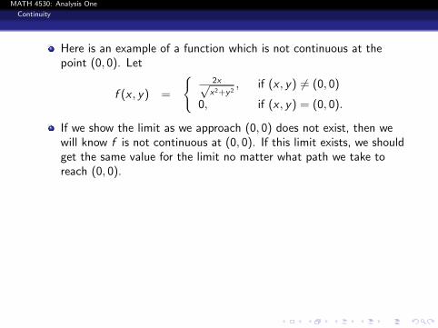
Here is an example of a function which is not continuous at thepoint (0, 0). Let
f (x , y) =
{2x√x2+y2
, if (x , y) 6= (0, 0)
0, if (x , y) = (0, 0).
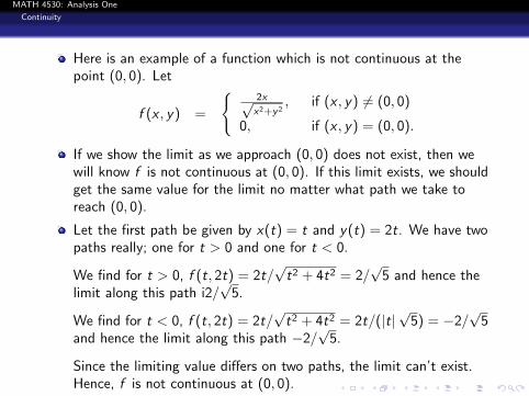
If we show the limit as we approach (0, 0) does not exist, then wewill know f is not continuous at (0, 0). If this limit exists, we shouldget the same value for the limit no matter what path we take toreach (0, 0).
Let the first path be given by x(t) = t and y(t) = 2t. We have twopaths really; one for t > 0 and one for t < 0.
We find for t > 0, f (t, 2t) = 2t/√t2 + 4t2 = 2/
√5 and hence the
limit along this path i2/√
5.
We find for t < 0, f (t, 2t) = 2t/√t2 + 4t2 = 2t/(|t|
√5) = −2/
√5
and hence the limit along this path −2/√
5.
Since the limiting value differs on two paths, the limit can’t exist.Hence, f is not continuous at (0, 0).
MATH 4530: Analysis One
Continuity
Here is an example of a function which is not continuous at thepoint (0, 0). Let
f (x , y) =
{2x√x2+y2
, if (x , y) 6= (0, 0)
0, if (x , y) = (0, 0).
If we show the limit as we approach (0, 0) does not exist, then wewill know f is not continuous at (0, 0). If this limit exists, we shouldget the same value for the limit no matter what path we take toreach (0, 0).
Let the first path be given by x(t) = t and y(t) = 2t. We have twopaths really; one for t > 0 and one for t < 0.
We find for t > 0, f (t, 2t) = 2t/√t2 + 4t2 = 2/
√5 and hence the
limit along this path i2/√
5.
We find for t < 0, f (t, 2t) = 2t/√t2 + 4t2 = 2t/(|t|
√5) = −2/
√5
and hence the limit along this path −2/√
5.
Since the limiting value differs on two paths, the limit can’t exist.Hence, f is not continuous at (0, 0).

MATH 4530: Analysis One
Continuity
Prove f (x , y) = 2x2 + 3y2 is continuous at (2, 3).
Solution
We find f (2, 3) = 8 + 27 = 35. Consider
|(2x2 + 3y2)− 35| = |( 2(x − 2 + 2)2 + 3(y − 3 + 3)2 )− 35|= |2(x − 2)2 + 8(x − 2) + 8 + 3(y − 3)2 + 18(y − 3) + 27− 35|= |2(x − 2)2 + 8(x − 2) + 3(y − 3)2 + 18(y − 3)|≤ 2|x − 2|2 + 8|x − 2|+ 3|y − 3|2 + 18|y − 3|
Next, start by choosing a positive r < 1. Then we note if (x , y) is inBr (2, 3), we have |x − 2| ≤
√|x − 2|2 + |y − 3|2 < r implying
|x − 2| < r . In a similar way, we see |y − 3| < r also.
Thus, since r < 1 implies r2 < r , we can say
|(2x2 + 3y2)− 35| < 2r2 + 8r + 3r2 + 18r = 5r2 + 26r < 31r
Thus, if δ < min{1, ε/31}, |(2x2 + 3y2)− 35| < ε and we have continuityat (2, 3).
MATH 4530: Analysis One
Continuity
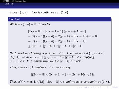
Prove f (x , y) = 2xy is continuous at (1, 4).
Solution
We find f (1, 4) = 8. Consider
|2xy − 8| = |2(x − 1 + 1) (y − 4 + 4)− 8|= |2(x − 1)(y − 4) + 2(y − 4) + 8(x − 1) + 8− 8|= |2(x − 1)(y − 4) + 2(y − 4) + 8(x − 1)|≤ 2|x − 1| |y − 4|+ 2|y − 4|+ 8|x − 1|
Next, start by choosing a positive r < 1. Then we note if (x , y) is inBr (1.4), we have |x − 1| ≤
√|x − 1|2 + |y − 4|2 < r implying
|x − 1| < r . In a similar way, we see |y − 4| < r also.
Thus, since r < 1 implies r2 < r , we can say
|(2xy − 8| < 2r2 + 2r + 8r = 2r2 + 10r < 12r
Thus, if δ < min{1, ε/12}, |2xy − 8| < ε and we have continuity at (1, 4).
MATH 4530: Analysis One
Continuity
Homework 32
32.1 Let f be a function whose second derivative is continuous. Provea. if f ′′(p) > 0 then f ′(x) increases locally at p. Discuss how thegraph of the function looks locally at p.b. if f ′′(p) < 0 then f ′(x) decreases locally at p. Discuss how thegraph of the function looks locally at p.
32.2 Let f (x , y) = 6x2 + 9y2. Prove f is continuous at (2, 3).
32.3 Let f (x , y) = 2xy + 3y2. Prove f is continuous at (1, 2).
32.4 Let f (x , y) = 5xy + 4x2. Prove f is continuous at (−2,−1).