jane liu mike west - duke universityftp.stat.duke.edu/workingpapers/99-14.pdfcom bined parameter and...

Combined parameter and state

estimation in simulation-based �ltering

Jane Liu & Mike West

Abstract

We discuss simulation-based sequential analysis { or particle �lter-

ing { in dynamic models, with a focus on sequential Bayesian learning

about time-varying state vectors and �xed model parameters simul-

taneously. This includes a general approach that combines old ideas

of smoothing using kernel methods with newer ideas of auxiliary par-

ticle �ltering. We highlight speci�c smoothing approaches that have

interpretation as adding \arti�cial evolution noise" to �xed model pa-

rameters at each time point to address problems of sample attrition

and prior:data con ict. We introduce a new approach that permits

such smoothing and regeneration of sample points of model parameters

without the \loss of historical information" inherent in earlier meth-

ods; this is achieved using shrinkage modi�cations of kernel smooth-

ing, as introduced by the second author in the early 1990s. Following

some theoretical development, discussion and a small simulated exam-

ple to demonstrate its eÆcacy, we report some experiences in using

the method in a challenging application in multivariate dynamic fac-

tor models for �nancial time series, as recently studied using MCMC

methods by authors, their collaborators, and other researchers. Some

summary comments and comparisons with MCMC methods are given

in this applied context, and we conclude with some discussion of gen-

eral issues of practical relevance, and suggestions for further algorith-

mic development.

1 Introduction and Historical Perspective

Much of the recent and current interest in simulation-based methods of se-quential Bayesian analysis of dynamic models has been focused on improvedmethods of �ltering for time-varying state vectors. We now have quite e�ec-tive algorithms for time-varying states, as represented throughout this vol-ume. Variants of the auxiliary particle �ltering algorithm (Pitt and Shephard1999b), in particular, are of proven applied eÆcacy in quite elaborate models.However, the need for more general algorithms that deal simultaneously withboth �xed model parameters and state variables is practically pressing. Wesimply do not have access to eÆcient and e�ective methods of treating this

1

2 Jane Liu & Mike West

problem, especially in models with realistically large numbers of �xed modelparameters. It is a very challenging problem.

A short historical commentary will be of interest in leading into the de-velopments presented in this chapter. In the statistics literature per se,simulation-based �ltering can be seen as a natural outgrowth of converginginterests in the late 1980s and early 1990s. For several decades researchersinvolved in sequential analysis of dynamic models, in both statistics and var-ious engineering �elds, have been using discrete numerical approximations tosequentially updated posterior distributions in various \mixture modelling"frameworks. This literature has involved methods for both time-evolvingstates and �xed parameters, and is exempli�ed by the important class ofadaptive multi-process models used in Bayesian forecasting since the early1970s (Harrison and Stevens 1976, Smith and West 1983, West and Harri-son 1997). During the 1980s, this naturally led to larger-scale analyses usingdiscrete grids of parameter values, though the combinatorial \explosion" ofgrid sizes with increasing parameter dimension limited this line of develop-ment. Novel methods using eÆcient quadrature-based, adaptive numericalintegration ideas were introduced in the later 1980s (Pole 1988, Pole, Westand Harrison 1988, Pole and West 1990). This involved useful methods inwhich discrete grids { of both �xed model parameters and state variables {themselves change over time as data is processed, sequentially adapting thediscrete posterior approximations by generating new \samples" as well as as-sociated \weights." This work recognised the utility of the Markov evolutionequations of dynamic models in connection with the generation of new grids ofvalues for time-evolving state variables. It similarly recognised and addressedthe practically critical issues of \diminishing weights" on unchanging grids ofparameter values, and the associated need for some method of interpolationand smoothing to \regenerate" grids of values for �xed model parameters.In these respects, this adaptive deterministic approach naturally anticipatedfuture developments of simulation-based approaches. Again, however, param-eter dimension limited the broader applicability of such approaches.

The end of the 1980s saw a developing interest in simulation-based meth-ods. Parallel developments in the early 1990s eventually led to publication ofdi�erent but related approaches (West 1993a, West 1993b, Gordon, Salmondand Smith 1993). All such approaches involve methods of evolving and up-dating discrete sets of sampled state vectors, and the associated weights onsuch sampled values, as they evolve in time. It has become standard to referto sampled values as \particles." The above referenced works, and others,have again highlighted the utility of the convolution structure of Markovevolution equations for state variables in generating Monte Carlo samples oftime-evolving states. Most approaches recognise and attempt to address theinherent problems of degrading approximation accuracy as particulate repre-sentations are updated over time { the issues of particle \attrition" in resam-pling methods and of \weight degeneracy" in reweighting methods. These

Parameter and state estimation 3

issues are particularly acute in approaches that aim to deal with �xed modelparameters as part of an extended state vector. This was addressed in theapproaches of West (1993a,b). Openly recognising the need for some kind ofinterpolation/smoothing of \old" parameter particles to generate new values,this author used local smoothing based on modi�ed kernel density estimationmethods, the modi�cations being based on Bayesian reasoning and gearedtowards adjusting for the over-smoothing problems inherent in standard ker-nel methods. In later years, this approach has been used and elaborated.For example, it has been extended to include variable shapes of multivari-ate kernels to re ect changing patterns of dependencies among parameters indi�erent regions of parameter space (Givens and Raftery 1996), as explicitlyanticipated in West (1993a,b). A related approach may be referred to as the\arti�cial evolution" method for model parameters. This relates to the workof Gordon et al (1993), who introduced the idea of adding additional randomdisturbances { or \roughening penalities" { to sampled state vectors in an at-tempt to deal with the degeneracy issues. Extending this idea to �xed modelparameters leads to a synthetic method of generating new sample points forparameters via the convolution implied by this \arti�cial evolution." Thisneat, ad-hoc idea is easily implementable, but su�ers the obvious drawbackthat it \throws away" information about parameters in assuming them to betime-varying when they are, in fact, �xed. The same drawback arises in usingthe idea in its original form for dynamic states.

In this current chapter, we take as our starting point these methods of deal-ing with �xed model parameters, and address the issues of reconciling themand then embedding a generalised algorithm within a sequential auxiliary par-ticle �ltering context. Section 2 discusses particle �ltering for state variables,and describes the general framework for combined �ltering on parameters andstate variables. Section 3 focuses on the problems arising in simulation-based�ltering for parameters, reviews the kernel and arti�cial evolution methods,identi�es the inherent structural similarities in these methods, and then in-troduces a modi�ed and easily implemented approach that improves uponboth by resolving the problem of information loss they each imply. Return-ing to the general framework in Section 4, we describe a general algorithmthat extends the more-or-less standard auxiliary particle �ltering approach forstate variables to include model parameters. We give a simple example forillustration, and then, in Section 5, report on some experiences in using themethod in a challenging application in multivariate dynamic factor modelsfor �nancial time series. Section 6 concludes with some summary comments,discussion and suggestions for new research directions.


2 General Framework

2.1 Dynamic Model and Analysis Perspective

Assume a Markovian dynamic model for sequentially observed data vectors yt;(t = 1; 2; : : :); in which the state vector at time t is xt and the �xed parametervector is �: The model is speci�ed at each time t by the observation equationde�ning the observation density

p(ytjxt; �) (2.1)

and the Markovian evolution equation, or state equation, de�ning the tran-sition density

p(xtjxt�1; �): (2.2)

Each yt is conditionally independent of past states and observations given thecurrent state xt and the parameter �; and xt is conditionally independent ofpast states and observations given xt�1 and �: This covers a very broad classof practically interesting models (West and Harrison 1997).

Sequential Monte Carlo methods aim to sequentially update Monte Carlosample approximations to the sequences of posterior distributions p(xt; �jDt)where Dt = fDt�1;ytg is the information set at time t: Thus, at time t thisposterior is represented by a discrete sample of points and weights (the latterpossibly though not necessarily uniform weights). On observing the new ob-servation yt+1 it is desired to produce a sample from the \current" posteriorp(xt+1; �jDt+1): There have been numerous contributors to theoretical andapplied aspects of research in this area in recent years (West 1993b, Gor-don et al. 1993, Kitagawa 1998, Liu and Chen 1995, Berzuini, Best, Gilksand Larizza 1997, Pitt and Shephard 1999b) and the �eld has really growndramatically both within statistical sciences and in related �elds including,especially, various branches of engineering (Doucet 1998). The current vol-ume represents a comprehensive catalogue of recent and current work.

The most e�ective methods all utilise the state equation to generate sam-ple values of the current state vector xt+1 based on past sampled values ofthe state xt: This is critical to the utility and performance of discrete approx-imation methods, as the generation of new sets of states from what is usuallya continuous state transition density allows the posterior approximations to\move around" in the state space as the state evolves and new data are pro-cessed. We focus now exclusively on auxiliary particle �lters as developed inPitt and Shephard (1999b), variants of which are, in our opinion, the moste�ective methods currently available { though that may change as the �eldevolves.


2.2 Filtering for States

Consider a model with no �xed parameters, or in which � is assumed known,so that the focus is entirely on �ltering for the state vector. Standing at timet; suppose we have a sample of current states fx(1)

t ; :::;x(N)t g and associated

weights f!(1)t ; :::; !

(N)t g that together represent a Monte Carlo importance

sample approximation to the posterior p(xtjDt): This includes, of course, thespecial case of equal weights in which we have a direct posterior sample. Timeevolves to t + 1; we observe yt+1; and want to generate a sample from theposterior p(xt+1jDt+1): Theoretically,

p(xt+1jDt+1) / p(yt+1jxt+1)p(xt+1jDt) (2.3)

where p(xt+1jDt) is the prior density of xt+1 and p(yt+1jxt+1) is the likeli-hood function. The second term here { the prior for the state at time t+1 {is implied by the state equation as

Rp(xt+1jxt)p(xtjDt)dxt: Under the Monte

Carlo approximation to p(xtjDt); this integral is replaced by a weighted sum-

mation over the sample points x(k)t ; so that the required update in equation

(2.3) becomes

p(xt+1jDt+1) / p(yt+1jxt+1)NXk=1

!(k)t p(xt+1jx(k)

t ): (2.4)

To generate Monte Carlo approximations to this density, an old and naturalidea is to sample from p(xt+1jx(k)

t ) for k = 1; :::; N , evaluate the corresponding

values of the weighted likelihood function !(k)t p(yt+1jxt+1) at each draw, and

then use the normalised weights as the new weights of the samples. Thisbasic \particle �lter" is an importance sampling method closely related tothose of West (1993a,b). A key problem is that the sampled points comefrom the current prior of xt+1 and the resulting weights may be very small onmany points in cases of meaningful separation of the prior and the likelihoodfunction based on yt+1: West (1993a,b) developed an e�ective method ofadaptive importance sampling to address this. The idea of auxiliary particle�ltering (see Pitt and Shephard, 1999b, and the chapter by these authors inthis volume) is similar in spirit but has real computational advantages; thisworks as follows. Incorporate the likelihood function p(yt+1jxt+1) under thesummation in equation (2.4) to give

p(xt+1jDt+1) /NXk=1

!(k)t p(xt+1jx(k)

t )p(yt+1jxt+1)

and generate samples of the current state as follows. For each k = 1; : : : ; N;select an estimate �

(k)t+1 of xt+1; such as the mean or mode of p(xt+1jx(k)

t ):

Evaluate the weights g(k)t+1 / !

(k)t p(yt+1j�(k)t+1): A large value of g

(k)t+1 indicates

that x(k)t ; when \evolving" to time t + 1; is likely to be more consistent


with the datum yt+1 than otherwise. Then indicators j are sampled with

probabilities proportional to g(j)t+1; and values x

(j)t+1 of the current state are

drawn from p(xt+1jx(j)t ) based on these \auxiliary" indicators. These sampled

states are essentially importance samples from the time t + 1 posterior andhave associated weights

!(j)t+1 =

p(yt+1jx(j)t+1)

p(yt+1j�(j)t+1)

: (2.5)

Posterior inferences at time t + 1 can be based directly on these sampledvalues and weights, or we may resample according to the importance weights!(j)t+1 to obtain an equally weighted set of states representing a direct Monte

Carlo approximation to the required posterior in equation (2.3).

2.3 Filtering for States and Parameters

In the general model with �xed parameters �; extend the sample-based frame-work as follows. Standing at time t; we now have a combined sample

fx(j)t ; �

(j)t : j = 1; : : : ; Ng

and associated weightsf!(j)

t : j = 1; : : : ; Ngrepresenting an importance sample approximation to the time t posteriorp(xt; �jDt) for both parameter and state. Note that the t suÆx on the �samples here indicate that they are from the time t posterior, not that �is time-varying. Time evolves to t + 1; we observe yt+1; and now want togenerate a sample from p(xt+1; �jDt+1): Bayes' theorem gives this as

p(xt+1; �jDt+1) / p(yt+1jxt+1; �)p(xt+1; �jDt)

/ p(yt+1jxt+1; �)p(xt+1j�;Dt)p(�jDt);

(2.6)

where the form chosen in the last equation makes explicit the notion that thetheoretical density function p(�jDt) is an important ingredient in the update.

If � were known, equation (2.6) simpli�es: p(�jDt) is degenerate and wedrop the known parameter from the conditioning statements. This leads toequation (2.3) and the auxiliary particle method applies for �ltering on thestate vector. Otherwise, it is now explicit that we have to deal with theproblem of not knowing the form of the theoretical density function p(�jDt)in order to obtain combined �ltering on the parameter and the state. Thenext section reviews the two main historical approaches.


3 The Treatment of Model Parameters

3.1 Arti�cial Evolution of Parameters

In dealing with time-varying states, Gordon et al (1993) suggested an ap-proach to reducing the sample degeneracy/attrition problem by adding smallrandom disturbances (referred to as \roughening penalties") to state particlesbetween time steps, in addition to any existing evolution noise contributions.In the literature since then, this idea has been extrapolated to �xed modelparameters. One version of the idea adds small random perturbations to allthe parameter particles under the posterior at each time point before evolvingto the next. This speci�c method has an interpretation as arising from anextended model in which the model parameters are viewed as if they are, infact, time-evolving { an \arti�cial evolution." That is, consider a di�erentmodel in which � is replaced by �t at time t; and simply include �t in an aug-mented state vector. Then add an independent, zero-mean normal incrementto the parameter at each time. That is,

�t+1 = �t + �t+1�t+1 � N(0;W t+1) (3.1)

for some speci�ed variance matrix W t+1 and where �t and �t+1 are condi-tionally independent given Dt:With the model recast with the correspondingaugmented state vector, the standard �ltering methods for states alone, suchas the auxiliary particle �lter, now apply. The key motivating idea is thatthe arti�cial evolution provides the mechanism for generating new parametervalues at each time step in the simulation analysis, so helping to address thesample attrition issue in reweighting methods that stay with the same sets ofparameter points between time steps.

Among the various issues and drawbacks of this approach, the key one issimply that �xed model parameters are, well, �xed! Pretending that they arein fact time-varying implies an arti�cial \loss of information" between timepoints, resulting in posteriors that are, eventually, far too di�use relative tothe theoretical posteriors for the actual �xed parameters. To date there hasbeen no resolution of this issue: if one adopts a model in which all parametersare subject to independent random shocks at each time point, the precisionof resulting inferences is inevitably limited.

However, an inherent interpretation in terms of kernel smoothing of par-ticles leads to a modi�cation of this arti�cial evolution method in which theproblem of information loss is avoided. First we discuss the basic form ofkernel smoothing as introduced and developed in West (1993).


3.2 Kernel Smoothing of Parameters

Understanding the imperative to develop some method of smoothing for ap-proximation of the required density p(�jDt) in equation (2.6), West (1993b)developed kernel smoothing methods that provided the basis for rather e�ec-tive adaptive importance sampling techniques. This represented extension tosequential analysis of basic mixture modelling ideas in West (1993a).

Standing at time t; suppose we have current posterior parameter samples�(j)t and weights !

(j)t ; (j = 1; :::; N); providing a discrete Monte Carlo approx-

imation to p(�jDt): Again remember that the t suÆx on � here indicates thatthe samples are from the time t posterior; � is not time-varying. Write �tand V t for the Monte Carlo posterior mean and variance matrix of p(�jDt);

computed from the Monte Carlo sample �(j)t with weights !

(j)t : The smooth

kernel density form of West (1993a,b) is given by

p(�jDt) �NXj=1

!(j)t N(�jm(j)

t ; h2V t) (3.2)

with the following de�ning components. First, N(�jm;S) is a multivariatenormal density mean m and variance matrix S; so that the above density isa mixture of N(�jm(j)

t ; h2V t) distributions weighted by the sample weights

!(j)t : Kernel rotation and scaling uses V t; the Monte Carlo posterior variance,

and the overall scale of kernels is a function of the smoothing parameterh > 0: Standard density estimation methods suggest that h be chosen asa slowly decreasing function of N; so that kernel components are naturallymore concentrated about their locations m

(j)t for larger N: West (1993a,b)

suggests taking slightly smaller values than the conventional kernel methodsas a general rule. As we discuss below, our new work has led to a quitedi�erent perspective on this issue.

The kernel locations m(j)t are speci�ed using a shrinkage rule introduced

by West (1993a,b). Standard kernel methods would suggest m(j)t = �

(j)t so

that kernels are located about existing sample values. However, this resultsin a kernel density function that is over-dispersed relative to the posteriorsample, in the sense that the variance of the resulting mixture of normalsis (1 + h2)V t; always larger than V t. This is a most signi�cant aw in thesequential simulation; an over-dispersed approximation to p(�jDt) will leadto an over-dispersed approximation to p(�jDt+1); and the consequent \loss ofinformation" will build up as the operation is repeated at future times. Tocorrect this, West (1993a,b) introduced the novel idea of shrinkage of kernellocations. Take

m(j)t = a�

(j)t + (1� a)�t (3.3)

where a =p1� h2:With these kernel locations, the resulting normal mixture

retains the mean �t and now has the correct variance V t; hence the over-dispersion is trivially corrected.


3.3 Reinterpreting Arti�cial Parameter Evolutions

The undesirable \loss of information" implicit in equation (3.1) can be easily

quanti�ed. The Monte Carlo approximation f�(j)t ; !(j)t g to p(�jDt) has mean

�t and variance matrix V t: Hence, in the evolution in equation (3.1) with theinnovation �t+1 independent of �t as proposed, the implied prior p(�t+1jDt)has the correct mean �t but variance matrix V t+W t+1: The loss of informa-tion is explicitly represented by the component W t+1: Now, there is a closetie-in between this method and the kernel smoothing approach. To see thisclearly, note that the Monte Carlo approximation to p(�t+1jDt) implied byequation (3.1) is also a kernel form, namely

p(�t+1jDt) �NXj=1

!(j)t N(�t+1j�(j)t ;W t+1) (3.4)

and this, as we have seen, is over-dispersed relative to the required or \target"variance V t:

It turns out that we can correct for this over-dispersion as follows. Thekey is to note that our kernel method is e�ective due to the use of locationshrinkage. This shrinkage pushes samples �(j)t values towards their mean �tbefore adding a small degree of \noise" implied by the normal kernel. Thissuggests that the arti�cial evolution method should be modi�ed by introduc-ing correlations between �t and the random shock �t+1: Assuming a non-zerocovariance matrix, note that the arti�cial evolution equation (3.1) implies

V (�t+1jDt) = V (�tjDt) +W t+1 + 2C(�t; �t+1jDt):

To correct to \no information lost" implies that we set

V (�t+1jDt) = V (�tjDt) = V t;

which then impliesC(�t; �t+1jDt) = �W t+1=2:

Hence there must be a structure of negative correlations to remove the un-wanted information loss e�ect. In the case of approximate joint normalityof (�t; �t+1jDt); this would then imply the conditional normal evolution inwhich

p(�t+1j�t) = N(�t+1jAt+1�t + (I �At+1)�t; (I �A2t+1)V t) (3.5)

where At+1 = I �W t+1V�1t =2:

The resulting Monte Carlo approximation to p(�t+1jDt) is then a gener-alised kernel form with complicated shrinkage patterns induced by the shrink-age matrix At+1: We restrict here to the very special case in which the evo-lution variance matrix W t+1 is speci�ed using a standard discount factortechnique. Speci�cally, take

W t+1 = V t(1

Æ� 1)


where Æ is a discount factor in (0; 1]; typically around 0:95�0:99: In this case,At+1 = aI with a = (3Æ � 1)=2Æ and the conditional evolution density abovereduces

p(�t+1j�t) � N(�t+1ja�t + (1� a)�t; h2V t) (3.6)

where h2 = 1 � a2; so that h2 = 1 � ((3Æ � 1)=2Æ)2; and we note thata =

p1� h2: The resulting Monte Carlo approximation to p(�t+1jDt) is then

precisely of the kernel form of equation (3.2), but now with a controllingsmoothing parameter h speci�ed directly via the discount factor.

We therefore have a version of the method of Gordon et al (1993) applied toparameters that connects directly with kernel smoothing with shrinkage. Thisjusti�es the basic idea of an arti�cial evolution for �xed model parameters ina modi�cation that removes the problem of information loss over time.

Note also that the modi�ed arti�cial evolution model of equation (3.6) maybe adopted directly, without reference to the motivating discussion involvingnormal posteriors. This is clear from the following general result. Supposep(�tjDt) has a �nite mean �t and variance matrix V t; whatever the global

form of the distribution may be. Suppose in addition that �t+1 is generatedby the evolution model speci�ed by equation (3.6). It is then easily seen thatthe mean and variance matrix of the implied marginal distribution p(�t+1jDt)are also �t and V t: Hence the connection with kernel smoothing with shrink-age, and the adjustment to �x the problem of information loss over time inarti�cial evolution approaches, is quite general. Note �nally that the frame-work provides a direct method of specifying the scale of kernels via the singlediscount factor Æ; as h (and a) are then simply determined. Generally, ahigher discount factor { around 0.99 { will be relevant.

4 A General Algorithm

Return now to the general �ltering problem, that of sampling the poste-rior in equation (2.6). We have available the Monte Carlo sample (x

(j)t ; �

(j)t )

and weights !(j)t (j = 1; : : : ; N); representing the joint posterior p(xt; �jDt):

Again, the suÆx t on the parameter samples indicates the time t poste-rior, not time-variation. We adopt the kernel form of equation (3.2) as themarginal density for the parameter, following the earlier discussion. Withthe equivalent interpretation of this as arising from an arti�cial evolutionwith correlation structure, as just discussed, we can now apply an extendedversion of the auxiliary particle �lter algorithm, incorporating the parameterwith the state. The resulting general algorithm runs as follows.

1. For each j = 1; :::; N , identify the prior point estimates of (xt; �) given

by (�(j)t+1;m

(j)t ) where

�(j)t+1 = E(xt+1jx(j)

t ; �(j)t ):


may be computed from the state evolution density and m(j)t = a�

(j)t +

(1� a)�t is the jth kernel location from equation (3.3).

2. Sample an auxiliary integer variable from the set f1; :::; Ng with prob-abilities proportional to

g(j)t+1 / !

(j)t p(yt+1j�(j)

t+1;m(j)t );

call the sampled index k:

3. Sample a new parameter vector �(k)t+1 from the kth normal component of

the kernel density, namely

�(k)t+1 � N(�jm(k)

t ; h2V t):

4. Sample a value of the current state vector x(k)t+1 from the system equation

p(�jx(k)t ; �

(k)t+1):

5. Evaluate the corresponding weight

!(k)t+1 /

p(yt+1jx(k)t+1; �

(k)t+1)

p(yt+1j�(k)t+1;m

(k)t )

:

6. Repeat step (2)-(5) a large number of times to produce a �nal posterior

approximation (x(k)t+1; �

(k)t+1) with weights !

(k)t+1; as required.

Note that the Monte Carlo sample size N can be di�erent at each timepoint, if required. Also, we might be interested in over-sampling a ratherlarger set of values and then resampling according to the weights above inorder to produce an equally weighted �nal sample. Further, it is generallyappropriate to operate with parameters that are real-valued, when using thenormal kernel method. Hence we routinely deal with log variances ratherthan variances, logit transforms of parameters restricted to a �nite range {such as the autoregressive parameter in the following AR(1) example and thelater dynamic factor model { and so forth.

Example

As a simple example in which the sequential updating is available in closedform for comparison, consider the AR(1) model in which yt = xt; a scalar,with xt+1 � N(xt�; 1): Here � = �; a single parameter, and there is nounobserved state variable. Hence the focus is exclusively on the eÆcacy oflearning the parameter (steps 1 and 4 of the general algorithm above arevacuous).


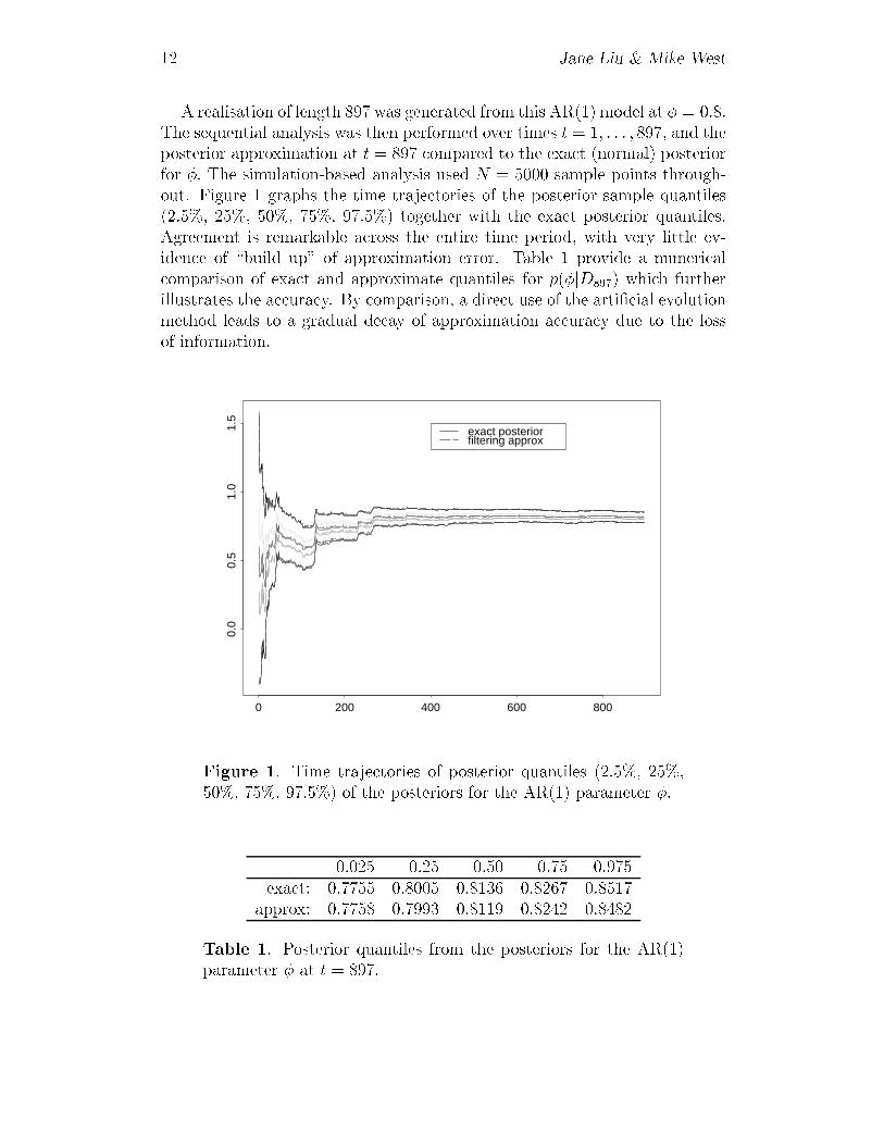
A realisation of length 897 was generated from this AR(1) model at � = 0:8:The sequential analysis was then performed over times t = 1; : : : ; 897; and theposterior approximation at t = 897 compared to the exact (normal) posteriorfor �: The simulation-based analysis used N = 5000 sample points through-out. Figure 1 graphs the time trajectories of the posterior sample quantiles(2.5%, 25%, 50%, 75%, 97.5%) together with the exact posterior quantiles.Agreement is remarkable across the entire time period, with very little ev-idence of \build up" of approximation error. Table 1 provide a numericalcomparison of exact and approximate quantiles for p(�jD897) which furtherillustrates the accuracy. By comparison, a direct use of the arti�cial evolutionmethod leads to a gradual decay of approximation accuracy due to the lossof information.

0 200 400 600 800

0.0

0.5

1.0

1.5

exact posteriorfiltering approx

Figure 1. Time trajectories of posterior quantiles (2.5%, 25%,50%, 75%, 97.5%) of the posteriors for the AR(1) parameter �:

0.025 0.25 0.50 0.75 0.975exact: 0.7755 0.8005 0.8136 0.8267 0.8517

approx: 0.7758 0.7993 0.8119 0.8242 0.8482

Table 1. Posterior quantiles from the posteriors for the AR(1)parameter � at t = 897:


5 Factor Stochastic Volatility Modelling

In studies of dynamic latent factor models with multivariate stochastic volatil-ity components, recent Bayesian work has developed both MCMC methodsand aspects of sequential analysis using versions of auxiliary particle �lteringfor states (Aguilar and West 2000, Pitt and Shephard 1999a). In these mod-els, the state variables are latent volatilities of both common factor processesand of residual/idiosyncratic random terms speci�c to observed time series.In the application in exchange rate modelling, forecasting and portfolio anal-ysis, Aguilar and West (1998) use MCMC methods to �t these complicateddynamic models to historical data, and then perform sequential particle �lter-ing over a long stretch of further data that provides the context for sequentialforecasting and portfolio construction. In that example, these authors �x afull set of constant model parameters at estimated values taken as the meansof posterior distributions based on the MCMC analysis of the initial (andvery long) data stretch. The results are very positive from the �nancial timeseries modelling viewpoint. For many practical purposes, an extension of thatapproach that involves periodic reanalysis of some recent historical data usingfull MCMC methods, followed by sequential analysis using auxiliary particle�ltering on just the time-varying states with model parameters �xed at mostrecently estimated values, is quite satisfactory. However, from the viewpointof the use of sequential simulation technology in more interesting, and com-plicated models, this setting provides a very nice and somewhat challengingtest-bed, especially when considering multivariate time series on moderatedimensions. Hence our interest in exploring the general sequential algorithmof the previous section in this context.

We adopt the context and notation of Aguilar and West (1998), noting thevery similar developments in Pitt and Shephard (1999a) and that our modelsare based on those of the earlier authors (Kim, Shephard and Chib 1998).Begin with a q�variate time series of observations, in yt; (t = 1; 2; : : :): Inour example, this is a vector of observed daily exchange rates of a set of q = 6national currencies relative to the US dollar. The dynamic latent factor modelwith multivariate stochastic volatility components is de�ned and structuredas follows.

At each time t; we have

yt = �t +Xf t + �t (5.1)

with the following ingredients.

� yt is the q-vector of observation and �t is a q-vector representing a locallevel of the series.

� X is a q � k matrix called the factor loadings matrix.


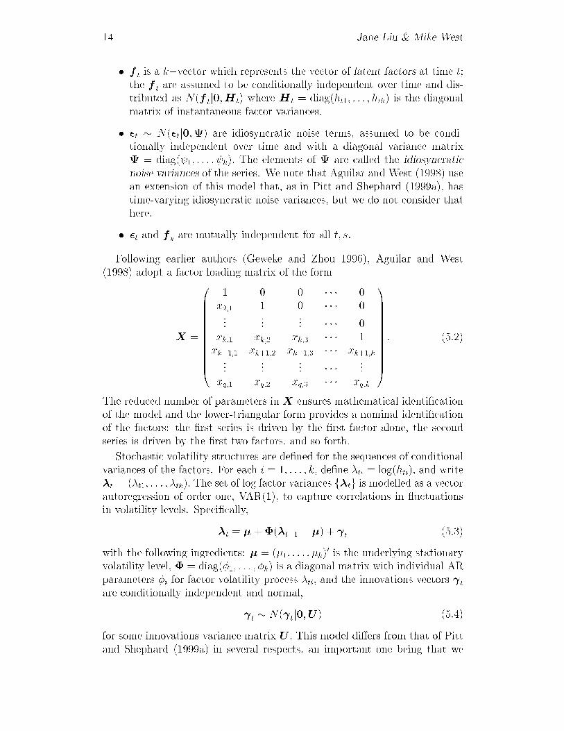
� f t is a k�vector which represents the vector of latent factors at time t;the f t are assumed to be conditionally independent over time and dis-tributed as N(f tj0;H t) where H t = diag(ht1; : : : ; htk) is the diagonalmatrix of instantaneous factor variances.

� �t � N(�tj0;) are idiosyncratic noise terms, assumed to be condi-tionally independent over time and with a diagonal variance matrix = diag( 1; : : : ; k): The elements of are called the idiosyncratic

noise variances of the series. We note that Aguilar and West (1998) usean extension of this model that, as in Pitt and Shephard (1999a), hastime-varying idiosyncratic noise variances, but we do not consider thathere.

� �t and f s are mutually independent for all t; s:

Following earlier authors (Geweke and Zhou 1996), Aguilar and West(1998) adopt a factor loading matrix of the form

X =

0BBBBBBBBBBBB@

1 0 0 � � � 0x2;1 1 0 � � � 0...

...... � � � 0

xk;1 xk;2 xk;3 � � � 1xk+1;1 xk+1;2 xk+1;3 � � � xk+1;k...

...... � � � ...

xq;1 xq;2 xq;3 � � � xq;k

1CCCCCCCCCCCCA

: (5.2)

The reduced number of parameters in X ensures mathematical identi�cationof the model and the lower-triangular form provides a nominal identi�cationof the factors: the �rst series is driven by the �rst factor alone, the secondseries is driven by the �rst two factors, and so forth.

Stochastic volatility structures are de�ned for the sequences of conditionalvariances of the factors. For each i = 1; : : : ; k; de�ne �ti = log(hti); and write�t = (�t1; : : : ; �tk): The set of log factor variances f�tg is modelled as a vectorautoregression of order one, VAR(1), to capture correlations in uctuationsin volatility levels. Speci�cally,

�t = �+�(�t�1 � �) + t (5.3)

with the following ingredients: � = (�1; : : : ; �k)0 is the underlying stationary

volatility level, � = diag(�1; : : : ; �k) is a diagonal matrix with individual ARparameters �i for factor volatility process �ti; and the innovations vectors t

are conditionally independent and normal,

t � N( tj0;U) (5.4)

for some innovations variance matrix U : This model di�ers from that of Pittand Shephard (1999a) in several respects, an important one being that we


allow non-zero o�-diagonal entries in U to estimate dependencies in changesin volatility patterns across the factors. This turns out to be empiricallysupported and practically relevant in short-term exchange rate modelling. Wenote that Aguilar and West (1998) also develop stochastic volatility modelcomponents for the variances of the idiosyncratic errors, but we do notexplore that here.

We analyse the one-day-ahead returns on exchange rates over a period ofseveral years in the 1990s, as in Aguilar and West (1998). Taking sti as thespot rate in US dollars for currency i on day t; the returns are simply yti =sti=st�1;i � 1 for currency i = 1; : : : ; q = 6: The currencies are, in order, theDeutschmark/Mark (DEM), Japanese Yen (JPY), Canadian Dollar (CAD),French Franc (FRF), British Pound (GBP) and Spanish Peseta (ESP). Herewe explore analysis of the returns over the period 12/1/92 to 8/9/96, a totalof 964 observations. We adopt the model as structured above, and take anassumedly �xed return level � = �:

We �rst performed intensive Bayesian analysis of the �rst 914 observationsusing the MCMC simulation approach of Aguilar and West (1998). At t =914; we then have a full sample from the actual posterior, based on data upto that time point, for all past latent factors, their volatilities, and all �xedmodel parameters. In terms of proceeding ahead sequentially, we identify therelevant state variables and parameters as follows. First note that we canreduce the model equation (5.1) by integrating out the latent factors to givethe conditional observation distribution

yt � N(ytj0;XH tX0 +): (5.5)

Now introduce the de�nitions of the state variable

xt �H t

at time t; and the �xed model parameters

� = fX;;�;�;Ug:In our example, the state variable xt is 3�dimensional, and the parameter� is 36�dimensional. As we discuss below, the sequential component of thestudy reported here treats U as �xed at a value based on the MCMC analysisof the �rst 914 observations, so that � reduces to 30 free model parameters,and the posterior at each time point is in 33 dimensions. For reference, theestimate of U is

E(U jD914) =

0B@0:0171 0:0027 0:00090:0027 0:0194 0:00130:0009 0:0013 0:0174

1CA

based on the initial MCMC analysis over t = 1; : : : ; 914: The posterior stan-dard deviations of elements of U at t = 914 are all of the order of 0.001-0.003,


865 915 955−0.01

−0.005

0

0.005

0.01

0.015

0.02

0.025DEM

time (day)865 915 955

−0.015

−0.01

−0.005

0

0.005

0.01

0.015JPY

time (day)865 915 955

−8

−6

−4

−2

0

2

4

6x 10

−3 CAD

time (day)

865 915 955−0.01

−0.005

0

0.005

0.01

0.015

0.02

0.025FRF

time (day)865 915 955

−0.015

−0.01

−0.005

0

0.005

0.01

0.015GBP

time (day)865 915 955

−0.01

−0.005

0

0.005

0.01

0.015

0.02ESP

time (day)

Figure 2. Exchange rate time series

so there is a fair degree of uncertainty about U that is being ignored in thesequential analysis and comparison.

To connect with the general dynamic model framework, note that we nowhave the observation equation (2.1) de�ned by the model equation (5.5),and the evolution equation (2.2) given implicitly by the stochastic volatilitymodel equations (5.3) and (5.4). We can now apply the general sequential�ltering algorithm, and do so starting at time t = 914 with the full posteriorp(x914; �jD914) available as a large Monte Carlo sample based on the MCMCanalysis of all the data up to that time. It is relevant to note that the contexthere { with an informed prior p(x914; �jD914) based on past data, is preciselythat facing practical analysts in many �elds in which further analysis, at leastover short stretches of data, is required to be sequential. As noted above, wemake one change: for reasons discussed below we �x the VAR(1) innovationsvariance matrix U at the estimate E(U jD914) and so the parameter � isreduced by removal of U : Hence the particle �ltering applies to the 3 statevariables at each time point and the 30 model parameters. We then proceedto analyse further data, sequentially, over t = 915; 916; : : : : Figure 2 displaysa stretch of the data running from t = 864 to t = 964 with t = 914 marked.Our sequential �ltering methods produces Monte Carlo approximations to


each p(xt; �jDt) over t = 915; 916; : : : : Throughout the analysis, the MonteCarlo sample size is �xed at N = 9000 at each step. The kernel shrinkage andshapes are de�ned via the discount factor Æ = 0:99 which implies a = 0:995and h = 0:1: A �nal technical point to note is that we operate with the kernelmethod on parameters transformed so that normal kernels are appropriate;thus each of the �j and �j parameters is transformed to the logit scale, andthe variance parameters j are logged (this follows West 1993a,b).

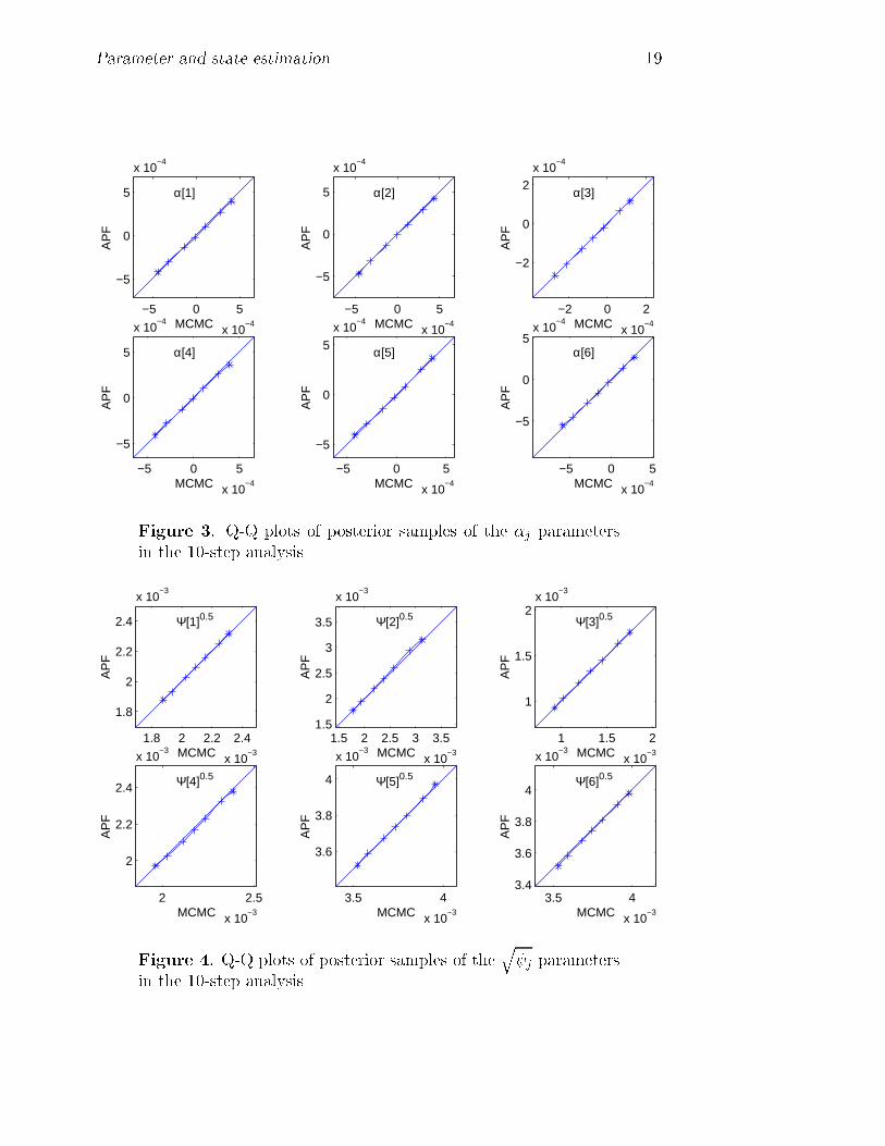
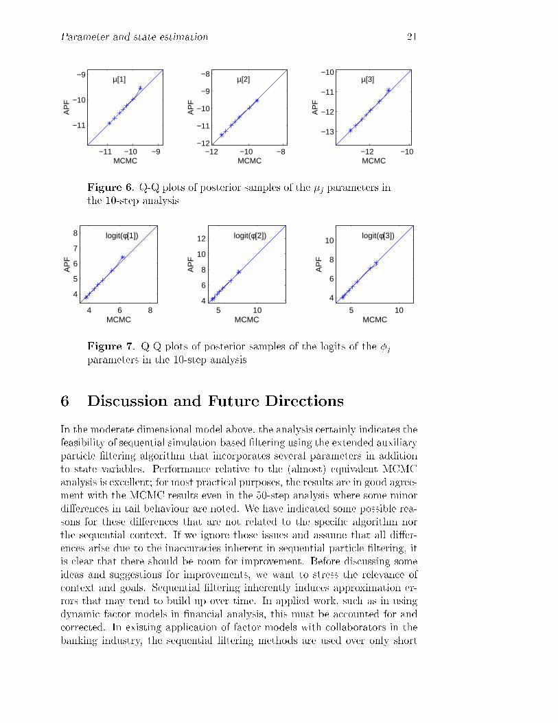
Our experiences in this study mirror those of using the straight auxiliaryparticle �ltering method when the parameters are assumed �xed (Aguilar andWest 2000). That is, �ltering on the volatilities is a more-or-less standardproblem, and the state variable is in only 3 dimensions so performance isexpected to be excellent. The questions of accuracy and performance in theextended context with a larger number of parameters are now much moreinteresting, however, due to the diÆculties inherent in dealing with discretesamples in higher dimensional parameter spaces. Inevitably, the accuracy ofapproximation is degraded relative to simple �ltering on two or three time-evolving states. One way to de�ne \performance" here is via comparison ofthe sequentially computed Monte Carlo approximations to posteriors withthose based on a full MCMC analysis that re�ts the entire data set up tospeci�ed time points of interest. Our discussion here focuses speci�cally onthis aspect in connection with inferences on the �xed model parameters. Fora chosen set of times during the period of 50 observations between t = 914and 964 we re-ran the full MCMC analysis of the factor model based on allthe data up to that time point, and explored comparisons with the sequential�ltering-based approximations in which we begin �ltering at t = 914: At anytime t the posterior from the MCMC analysis plays the role of the \true"posterior, or at least the \gold standard" by which to assess the performanceof the �ltering algorithm. Some relevant summaries appear in Figures 3 to12 inclusive. The �rst set, Figures 3{7, display summaries of the univariatemarginal posterior distributions at t = 924: We refer to this as the 10-stepanalysis, as the sequential �lter is run for just 10 steps from the startingposition at t = 914: For each of the 30 �xed parameters, we display quantileplots comparing quantiles of the approximate posteriors from the MCMC andsequential analyses. The graphs indicate (with crosses) the posterior quantilesat 1, 5, 25, 50, 75, 95 and 99% of the posteriors, graphing the �ltering-basedquantiles versus those from the MCMC. The y = x line is also drawn. Fromthese graphs, it is evident that posterior margins are in excellent agreement(we could have added approximate intervals to these plots, based on methodsof Bayesian density estimation, to represent uncertainty about the estimatedquantile functions; for the large sample sizes of 9000 here, such intervals areextremely narrow except in the extreme tails, and just obscure the plots.)The poster margins computed by the auxiliary particle �ltering (APF) andMCMC analyses are the same for all practical purposes. Only in the veryextreme upper tail of two of the VAR model parameters { �1 and the logit


of �1 { are there any deviations at all, and here the APF posterior is veryslightly heavier tailed than that from the MCMC, but the di�erences arehardly worth a mention.

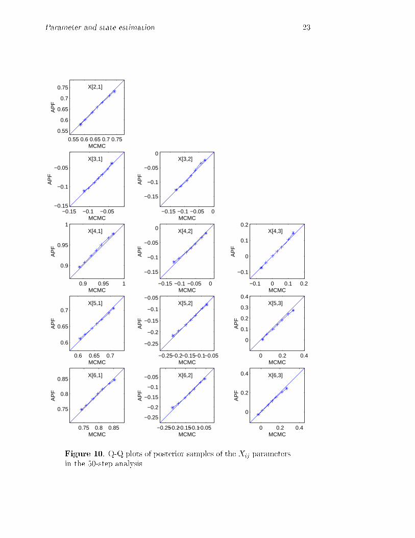
The remaining graphs, Figures 8{12, display similar quantile plots com-paring the APF and MCMC posteriors t = 964: This provides a similarcomparison but now for a 50-step analysis, the sequential �lter running for50 time points from the starting position at t = 914: Again we see a highdegree of concordance in general, although the longer �ltering period has in-troduced some discrepancies between the marginal posteriors, especially inthe extreme tails of several of the margins. Some of the bigger apparentdi�erences appear in the parameters � and � of the VAR volatility modelcomponent, indicated in Figures 11 and 12. Also noteworthy is the fact thatthis period of 50 observations includes a point at around t = 940 where theseries exhibits a real outlier, peaking markedly in the DEM, FRF, ESP andCAN series. Such events challenge sequential methods of any kind, and mayplay a role here in inducing small additional inaccuracies in the APF approx-imations by skewing the distribution of posterior weights at that time point.We do have ranges of relevant methods for model monitoring and adaptationto handle such events (West 1986, West and Harrison 1986, 1989 and 1997)though such methods are not applied in this study.

One additional aspect of the analysis worth noting is that the distributionsof the sets of sequentially updated weights !(j)

t remain very well-behavedacross the 50 update points. The shape is smooth and unimodal near thenorm of 1=N = 1=9000; with few weights deviating really far at all. Evenat the outlier point the maximum weight is only is 0.004, fewer than 200 ofthe 9000 weights are less than 0:1=9000; and only 16 exceed 10=9000: All inall, we can view the analysis as indicating the utility of the �ltering approacheven over rather longer time intervals.

As earlier mentioned, the sequential simulation analysis �xes the volatilityinnovations variance matrix U at its prior mean E(U jD914): This is becausewe have no easy way of incorporating a structured set of parameters such asU in the kernel framework { normal distributions do not apply to symmetricpositive de�nite matrices of parameters. It may be that �xing this set ofparameters induces some inaccuracies in the �ltering analysis compared to theMCMC analysis. With this in mind, we should expect to see some di�erencesbetween the APF posterior and the MCMC, and these di�erences can beexpected to be most marked in the margins for the volatility model parameters� and, most particularly, �: The largest di�erences in the 50-step analysisdo indeed relate to �; suggesting that some of the di�erences generally mayindeed be due to the lack of proper accounting for the uncertainties about U :Looking ahead, it is of interest to anticipate developments of kernel methodsthat allow for such structuring { perhaps using normal kernels with elaboratereparametrisations, or perhaps with a combination of normal and non-normalkernels { though for the moment we have no way of doing this.


−5 0 5

x 10−4

−5

0

5

x 10−4

AP

F

MCMC

α[1]

−5 0 5

x 10−4

−5

0

5

x 10−4

AP

F

MCMC

α[2]

−2 0 2

x 10−4

−2

0

2x 10

−4

AP

F

MCMC

α[3]

−5 0 5

x 10−4

−5

0

5

x 10−4

AP

F

MCMC

α[4]

−5 0 5

x 10−4

−5

0

5

x 10−4

AP

F

MCMC

α[5]

−5 0 5

x 10−4

−5

0

5x 10

−4

AP

F

MCMC

α[6]

Figure 3. Q-Q plots of posterior samples of the �j parametersin the 10-step analysis

1.8 2 2.2 2.4

x 10−3

1.8

2

2.2

2.4

x 10−3

AP

F

MCMC

Ψ[1]0.5

1.5 2 2.5 3 3.5

x 10−3

1.5

2

2.5

3

3.5

x 10−3

AP

F

MCMC

Ψ[2]0.5

1 1.5 2

x 10−3

1

1.5

2x 10

−3

AP

F

MCMC

Ψ[3]0.5

2 2.5

x 10−3

2

2.2

2.4

x 10−3

AP

F

MCMC

Ψ[4]0.5

3.5 4

x 10−3

3.6

3.8

4

x 10−3

AP

F

MCMC

Ψ[5]0.5

3.5 4

x 10−3

3.4

3.6

3.8

4

x 10−3

AP

F

MCMC

Ψ[6]0.5

Figure 4. Q-Q plots of posterior samples of theq j parameters

in the 10-step analysis


0.55 0.6 0.65 0.7 0.75

0.55

0.6

0.65

0.7

0.75A

PF

MCMC

X[2,1]

−0.15 −0.1 −0.05−0.15

−0.1

−0.05

AP

F

MCMC

X[3,1]

0.9 0.95 1

0.9

0.95

1

AP

F

MCMC

X[4,1]

0.6 0.65 0.7

0.6

0.65

0.7

AP

F

MCMC

X[5,1]

0.75 0.8 0.85

0.75

0.8

0.85

AP

F

MCMC

X[6,1]

−0.15 −0.1 −0.05 0

−0.15

−0.1

−0.05

0

AP

F

MCMC

X[3,2]

−0.15 −0.1 −0.05 0

−0.15

−0.1

−0.05

0

AP

F

MCMC

X[4,2]

−0.25−0.2−0.15−0.1−0.05

−0.25

−0.2

−0.15

−0.1

−0.05

AP

F

MCMC

X[5,2]

−0.25−0.2−0.15−0.1−0.05

−0.25

−0.2

−0.15

−0.1

−0.05

AP

F

MCMC

X[6,2]

−0.1 0 0.1 0.2

−0.1

0

0.1

0.2

AP

F

MCMC

X[4,3]

0 0.2 0.4

0

0.1

0.2

0.3

0.4

AP

F

MCMC

X[5,3]

0 0.2 0.4

0

0.2

0.4

AP

F

MCMC

X[6,3]

Figure 5. Q-Q plots of posterior samples of the Xij parametersin the 10-step analysis


−11 −10 −9

−11

−10

−9A

PF

MCMC

µ[1]

−12 −10 −8−12

−11

−10

−9

−8

AP

F

MCMC

µ[2]

−12 −10

−13

−12

−11

−10

AP

F

MCMC

µ[3]

Figure 6. Q-Q plots of posterior samples of the �j parameters inthe 10-step analysis

4 6 8

4

5

6

7

8

AP

F

MCMC

logit(φ[1])

5 104

6

8

10

12

AP

F

MCMC

logit(φ[2])

5 10

4

6

8

10

AP

FMCMC

logit(φ[3])

Figure 7. Q-Q plots of posterior samples of the logits of the �jparameters in the 10-step analysis

6 Discussion and Future Directions

In the moderate dimensional model above, the analysis certainly indicates thefeasibility of sequential simulation-based �ltering using the extended auxiliaryparticle �ltering algorithm that incorporates several parameters in additionto state variables. Performance relative to the (almost) equivalent MCMCanalysis is excellent; for most practical purposes, the results are in good agree-ment with the MCMC results even in the 50-step analysis where some minordi�erences in tail behaviour are noted. We have indicated some possible rea-sons for these di�erences that are not related to the speci�c algorithm northe sequential context. If we ignore those issues and assume that all di�er-ences arise due to the inaccuracies inherent in sequential particle �ltering, itis clear that there should be room for improvement. Before discussing someideas and suggestions for improvements, we want to stress the relevance ofcontext and goals. Sequential �ltering inherently induces approximation er-rors that may tend to build up over time. In applied work, such as in usingdynamic factor models in �nancial analysis, this must be accounted for andcorrected. In existing application of factor models with collaborators in thebanking industry, the sequential �ltering methods are used over only short


−5 0 5

x 10−4

−5

0

5

x 10−4

AP

F

MCMC

α[1]

−5 0 5

x 10−4

−5

0

5

x 10−4

AP

F

MCMC

α[2]

−2 0 2

x 10−4

−2

0

2x 10

−4

AP

F

MCMC

α[3]

−5 0 5

x 10−4

−5

0

5

x 10−4

AP

F

MCMC

α[4]

−5 0 5

x 10−4

−5

0

5x 10

−4

AP

F

MCMC

α[5]

−5 0 5

x 10−4

−5

0

5x 10

−4

AP

F

MCMC

α[6]


1.8 2 2.2 2.4

x 10−3

1.8

2

2.2

2.4

x 10−3

AP

F

MCMC

Ψ[1]0.5

1.5 2 2.5 3 3.5

x 10−3

1.5

2

2.5

3

3.5

x 10−3

AP

F

MCMC

Ψ[2]0.5

1 1.5 2

x 10−3

1

1.5

2x 10

−3

AP

F

MCMC

Ψ[3]0.5

2 2.5

x 10−3

2

2.2

2.4

x 10−3

AP

F

MCMC

Ψ[4]0.5

3.5 4

x 10−3

3.6

3.8

4

x 10−3

AP

F

MCMC

Ψ[5]0.5

3.5 4

x 10−3

3.6

3.8

4

x 10−3

AP

F

MCMC

Ψ[6]0.5

Figure 9. Q-Q plots of posterior samples of theq j parameters

in the 50-step analysis


0.55 0.6 0.65 0.7 0.75

0.55

0.6

0.65

0.7

0.75

AP

F

MCMC

X[2,1]

−0.15 −0.1 −0.05−0.15

−0.1

−0.05

AP

F

MCMC

X[3,1]

0.9 0.95 1

0.9

0.95

1

AP

F

MCMC

X[4,1]

0.6 0.65 0.7

0.6

0.65

0.7

AP

F

MCMC

X[5,1]

0.75 0.8 0.85

0.75

0.8

0.85

AP

F

MCMC

X[6,1]

−0.15 −0.1 −0.05 0

−0.15

−0.1

−0.05

0

AP

F

MCMC

X[3,2]

−0.15 −0.1 −0.05 0

−0.15

−0.1

−0.05

0

AP

F

MCMC

X[4,2]

−0.25−0.2−0.15−0.1−0.05

−0.25

−0.2

−0.15

−0.1

−0.05

AP

F

MCMC

X[5,2]

−0.25−0.2−0.15−0.1−0.05

−0.25

−0.2

−0.15

−0.1

−0.05

AP

F

MCMC

X[6,2]

−0.1 0 0.1 0.2

−0.1

0

0.1

0.2

AP

F

MCMC

X[4,3]

0 0.2 0.4

0

0.1

0.2

0.3

0.4

AP

F

MCMC

X[5,3]

0 0.2 0.4

0

0.2

0.4

AP

F

MCMC

X[6,3]

Figure 10. Q-Q plots of posterior samples of the Xij parametersin the 50-step analysis


−11 −10 −9

−11

−10

−9

AP

F

MCMC

µ[1]

−12 −10 −8−12

−11

−10

−9

−8

AP

F

MCMC

µ[2]

−12 −10

−13

−12

−11

−10

AP

F

MCMC

µ[3]


4 6 8

4

5

6

7

8

AP

F

MCMC

logit(φ[1])

4 6 8

4

6

8A

PF

MCMC

logit(φ[2])

5 10

4

6

8

10

AP

F

MCMC

logit(φ[3])

Figure 12. Q-Q plots of posterior samples of the logits of the �jparameters in the 50-step analysis

time scales { the 5 days of a working week with daily time series such as theexchange rate returns here. This is coupled with periodic updating based ona full MCMC analysis of a longer historical stretch of data (i.e., MCMC atthe weekend based on the last several months of data). The horizon of 10days in the example is therefore very relevant, whereas the 50 day horizonis very long and perhaps unrealistic. In this context, the di�erences betweenthe �ltering-based and MCMC-based posterior quantile functions at lowertime steps are quite negligible relative to those at the longer time step. Thisexperience and perspective is consistent with our long-held view that sequen-tial simulation-based �ltering methods must always be combined with someform of periodic re-calibration based on o�-line analysis performed with muchmore computational time available than the �ltering methods are designed toaccommodate.

Some �nal comments relate to possible extensions of the �ltering algorithmthat may improve posterior approximations. Questions of accuracy and ad-equacy arise in connection with the approximation of (typical) posteriorsthat exhibit varying patterns of dependencies among parameters in di�erentregions of the parameter space, and also varying patterns of tail-weight. Dis-crete, sample-based approximations inevitably su�er problems of generating


points far enough into the tails of fatter-tailed posteriors, especially in higherdimensions. It is sometimes helpful to use fatter-tailed kernels, such as T ker-nels (West 1993a, West 1993b) but this does not often help much and goes noway to addressing the real need for more sensitive analytic approximation oflocal structure in the posterior; the kernel mixture of equation (3.2) is globalin that the mixture components are based on the same \global" shrinkage cen-ter �t and each have the same scales and shapes as determined by h2V t: Verylarge numbers of such kernels are needed to truly adequately approximateposteriors that may evidence tails of di�ering weight in di�erent dimensions(and fatter than normal tails), highly non-linear relationships among the pa-rameters and hence varying patterns of \local" scale and shape as we movearound in � space. We need to complement this suggestion with modi�cationsthat allow \di�erential shrinkage centers." West (1993a,b) discussed some ofthese issues, with suggestions about kernel methods with kernel-speci�c vari-ance matrices in components in particular, and this idea was developed andimplemented in certain non-sequential contexts in Givens and Raftery (1996).Development for implementation in sequential contexts remains an importantresearch challenge.

A simple example helps to highlight these issues and underscores somesuggestions for algorithmic extensions that follows. Consider a bimodal priorp(�jDt) in which one mode has the shape of a unit normal distribution andthe other that of a normal but with a much larger variance. In using akernel approximation based on a prior sample, we would expect to do verymuch better using bimodal mixture in which sample points \near" one modeare shrunk towards that mode, and with kernel scalings that are higher forpoints \near" the second mode. The existing global kernel method uses globalshrinkage to match the �rst two moments, but loses accuracy in less regularsituations as this example indicates.

A speci�c research direction that re ects these considerations completesour discussion. To begin, consider the existing framework and recall that anydensity function p(�tjDt) may be arbitrarily well approximated by a mixtureof normal distributions. Suppose therefore, for theoretical discussion, thatthe density has exactly such a form, namely

p(�tjDt) =RX

r=1

qrN(�tjbr;Br) (6.1)

for some parameters R and fqr; br;Br : r = 1; : : : ; Rg (these will all dependon t though this is not made explicit in the notation, for clarity). In thiscase, the mean �t and variance matrix V t are given by �t =

PRr=1 qrbr and

V t =PR

r=1 qrfBr + (br � �t)(br � �t)0g: Suppose also, again, that �t+1 isgenerated by the evolution model speci�ed by equation (3.6). It then easily


follows that the implied marginal density p(�t+1jDt) is of the form

p(�t+1jDt) =RX

r=1

qkN(�t+1jabr + (1� a)�t; a2Br + (1� a2)V t): (6.2)

Now, in general, this is not the same as the density of (�tjDt); though themean and variance matrix match as mentioned above. In practice, a will bequite close to 1 so that the two distributions will be close, but not preciselythe same in general. The exception is the case of a normal p(�tjDt); i.e., thecase R = 1; when both p(�tjDt) and p(�t+1jDt) are N(�j�t;V t): Otherwise,in the case of quite non-normal priors, the component means br will be quiteseparated, the local variance matrices Br quite di�erent in scale and struc-ture. Hence the location and scale/shape shrinkage e�ects in the componentsof the resulting mixture (6.2) tend to obscure the di�erences by the impliedshrinking/averaging.

This discussion, linking back to the important use of normality of �t inthe theoretical tie-up between arti�cial evolution methods and kernel meth-ods in Section 3.3, suggests the following development. Suppose that thedistribution p(�tjDt) is indeed exactly of the form of equation (6.2). To focuson \local" structure in this distribution, introduce the component indica-tor variable rt such that rt = r with probability qr (r = 1; : : : ; R): Then(�tjrt = r;Dt) � N(�jbr;Br): At this point we can apply the same line ofreasoning about an arti�cial evolution to smooth a set of �t samples, but nowexplicitly including the indicator rt provides a focus on the local structure.This suggests the modi�cation of the key evolution equation (3.6) to the localform

p(�t+1j�t; rt = r;Dt) � N(�t+1ja�t + (1� a)br; h2Br) (6.3)

where a; h are as earlier de�ned. This conditional distribution is such that theimplied marginal p(�t+1jDt) has precisely the same mixture form as p(�tjDt);so that the local structure is respected. This theoretical discussion thereforeindicates and opens up a direction for development that, if implemented, canbe expected to generate more accurate and eÆcient methods of smoothingposterior samples. To exploit this mixture theory will require, among otherthings, computationally and statistically eÆcient methods of identifying theparameters R and fqr; br;Br : r = 1; : : : ; Rg of the mixture in equation (6.1)based on an existing Monte Carlo sample (and weights) from that distribution.Some form of hierarchical clustering of sample points (and weights), such asutilised in West (1993a,b), will be needed, though a key emphasis lies oncomputational eÆciency so new clustering methods will be needed. Suchdevelopments, while challenging, will directly contribute in this context tousefully extend and improve the existing algorithms for sequential �lteringon both parameters and states in higher dimensional dynamic models.


Acknowledgements

The authors are grateful for comments and fruitful discussions with OmarAguilar, Simon Godsill, Neil Gordon, Pepe Quintana and an anonymous ref-eree. This work was performed under partial support of NSF grant DMS-9704432 (USA), and while the �rst author was a PhD student at Duke Uni-versity. The authors would also like to acknowledge the support of CDCInvestment Management Corporation.

References

Aguilar, O. and West, M. (2000). Bayesian dynamic factor models and port-folio allocation, Journal of Business and Economic Statistics.

Berzuini, C., Best, N. G., Gilks, W. R. and Larizza, C. (1997). Dynamic con-ditional independence models and Markov chain Monte Carlo methods,Journal of the American Statistical Association 92: 1403{1412.

Doucet, A. (1998). On sequential simulation-based methods for Bayesian�ltering, Technical report CUED/F-INFENG/TR 310, Department ofEngineering, Cambridge University.

Geweke, J. F. and Zhou, G. (1996). Measuring the pricing error of the arbi-trage pricing theory, The Review of Financial Studies 9: 557{587.

Givens, G. and Raftery, A. E. (1996). Local adaptive importance samplingfor multivariate densities with strong nonlinear relationships, Journal ofthe American Statistical Association 91: 132{141.

Gordon, N. J., Salmond, D. J. and Smith, A. F. M. (1993). Novel approach tonon-linear/non-Gaussian Bayesian state estimation, IEE Proceedings-F140: 107{113.

Harrison, P. J. and Stevens, C. F. (1976). Bayesian forecasting (with discus-sion), Journal of the Royal Statistical Society, Series B 38: 205{247.

Kim, S., Shephard, N. and Chib, S. (1998). Stochastic volatility: Likelihoodinference and comparison with arch models, Review of Economic Studies65: 361{393.

Kitagawa, G. (1998). Self-organising state space model, Journal of the Amer-ican Statistical Association 93: 1203{1215.

Liu, J. S. and Chen, R. (1995). Sequential Monte Carlo methods for dynamicsystems, Journal of the American Statistical Association 90: 567{576.


Pitt, M. and Shephard, N. (1999a). Analysis of time varying covariances: Afactor stochastic volatility approach, in J. O. Berger, J. M. Bernardo,A. P. Dawid and A. F. M. Smith (eds), Bayesian Statistics 5, UniversityPress, Oxford, pp. 547{570.

Pitt, M. and Shephard, N. (1999b). Filtering via simulation: Auxiliary parti-cle �lters, Journal of the American Statistical Association 94: 590{599.

Pole, A. (1988). Transfer response models: A numerical approach, in J. M.Bernardo, M. H. DeGroot, D. V. Lindley and A. F. M. Smith (eds),Bayesian Statistics 3, University Press, Oxford, pp. 733{746.

Pole, A. and West, M. (1990). EÆcient Bayesian learning in non-linear dy-namic models, Journal of Forecasting 9: 119{136.

Pole, A., West, M. and Harrison, P. J. (1988). Non-normal and non-lineardynamic Bayesian modelling, in J. C. Spall (ed.), Bayesian Analysis ofTime Series and Dynamic Models, Marcel Dekker, New York, pp. 167{198.

Smith, A. F. M. and West, M. (1983). Monitoring renal transplants: Anapplication of the multi-process Kalman �lter, Biometrics 39: 867{878.

West, M. (1986). Bayesian model monitoring, Journal of the Royal StatisticalSociety (Ser. B) 48: 70{78.

West, M. (1993a). Approximating posterior distributions by mixtures, Jour-nal of Royal Statistical Society 55: 409{422.

West, M. (1993b). Mixture models, Monte Carlo, Bayesian updating and dy-namic models, in J. H. Newton (ed.), Computing Science and Statistics:Proceedings of the 24th Symposium on the Interface, Interface Founda-tion of North America, Fairfax Station, Virginia, pp. 325{333.

West, M. and Harrison, P. J. (1986). Monitoring and adaptation in Bayesianforecasting models, Journal of the American Statistical Association81: 741{750.

West, M. and Harrison, P. J. (1989). Subjective intervention in formal models,Journal of Forecasting 8: 33{53.

West, M. and Harrison, P. J. (1997). Bayesian Forecasting and DynamicModels, 2nd edn, Springer-Verlag, New York.

jane liu mike west - duke universityftp.stat.duke.edu/workingpapers/99-14.pdfcom bined parameter and...

Documents