jean-christophe poggiale aix-marseille université mediterranean institute of oceanography u.m.r....

Jean-Christophe POGGIALE

Aix-Marseille UniversitéMediterranean Institute of Oceanography

U.M.R. C.N.R.S. 7249

Case 901 – Campus de Luminy – 13288 Marseille CEDEX [email protected]

Leicester – Feb. 2013

Mathematical formulation of ecological processes : a problem of scaleMathematical approach and ecological consequences

mailto:[email protected]

Outline

I – Mathematical systems with several time scales : singular perturbation theory and its geometrical framework

I-1) An example with three time scalesI-2) Some mathematical methodsI-3) Some comments on their usefulness : limits and extensions

II – Mathematical modelling – Processe formulation - Structure sensitivity

III – Several formulations for one process : a dynamical system approach

V – Conclusion


Example

A tri-trophic food chains model

22

11

1

yd

cyez

d

dz

zyd

cy

xb

axey

d

dy

yxb

ax

K

xrx

d

dx

where 1

Deng and Hines (2002)

de Feo and Rinaldi (1998)

Muratori and Rinaldi (1992)


Example

Some results

• Under some technical assumptions, there exists a singular homoclinic orbit.

• Under some technical assumptions, there exists a saddle-focus in the positive orthant.

• This orbit is a Shilnikov orbit.

• This orbit is contained in a chaotic attractor

These results are obtained “by hand”, by using ideas of the Geometrical Singular Perturbation theory (GSP)


Slow-Fast vector fields

yxgd

dy

yxfd

dx

,

,

0

0,,

y

yxfx

yxx * Top – down

,,

,,

yxgy

yxfx

,,,,

,*

*

yGyyxgy

yxx

Bottom – up


Example

How to deal with this multi-time scales dynamical system ?

1) Neglect the slow dynamics

2) Analyze the remaining systems (when slow variables are assumed to be constant)

3) Eliminate the fast variables in the slow dynamics and reduce the dimension

4) Compare the complete and reduced dynamics


Example


11

1

xb

axey

d

dy

yxb

ax

K

xrx

d

dx

0


?

?

Example


11

1

xb

axey

d

dy

yxb

ax

K

xrx

d

dx

0


Example



Geometrical Singular Perturbation theory (GSP)


Geometrical Singular Perturbation theory

The fundamental theorems : normal hyperbolicity theory

,,

,,

yxgy

yxfx

2

1

k

k

IRy

IRx

Def. : The invariant manifold M0 is normally hyperbolic if the linearization of the previous system at each point of M0 has exactly k2 eigenvalues on the imaginary axis.




Theorem (Fenichel, 1971) : if is small enough, there exists a manifold M1 close and diffeomorphic to M0. Moreover, it is locally invariant under the flow, and differentiable.

Theorem (Fenichel, 1971) : « the dynamics in the vicinity of the invariant manifold is close to the dynamics restricted on the manifolds ».




• Simple criteria for the normal hyperbolicity in concrete cases (Sakamoto, 1991)

• Good behavior of the trajectories of the differential system in the vicinity of the perturbed invariant manifold.

• Reduction of the dimension

• Powerful method to analyze the bifurcations for the reduced system and link them with the bifurcations of the complete system



Why do we need theorems ?

• Intuitive ideas used everywhere (quasi-steady state assumption, …)

• Complexity of the involved mathematical techniques




11

222121212

1111212121

NebPd

dP

NrNmNmd

dN

ParNNmNmd

dN

21 NNN

11

112121

11112112121

NebPd

dP

PNaNrNrrd

dN

ParNNmmNmd

dN

Slow-fast system




PeaNPdt

dP

aNPrNdt

dN

11

112121

11112112121

NebPd

dP

PNaNrNrrd

dN

ParNNmmNmd

dN

2112

21*2

2112

12*1 mm

NmN

mm

NmN

N

Nr

N

Nrr

*2

2

*1

1 N

Naa

*1

1t




2112

2121

*2

*1

1 ;mmN

ParrNNPN

PNNPeaPeaNPdt

dP

ParrPNNaNPrNdt

dN

;

;

11

1211

Fenichel theorem

where




• Theorems help to solve more complex cases where intuition is wrong

• Theorems provide a global theory which allows us to extend the results to non hyperbolic cases

• Theorems provide tools to analyse bifurcations on the slow manifold


Loss of normal hyperbolicity



A simple example

xyd

dyd

dx

x

y

Unstable

Solve the system :

0xx

2

00 2exp xyy

Dynamical bifurcation

? ? ?



A simple example

0xx

2

00 2exp xyy

20

0

0 0

2 ln

;

Kx

y

y K t x x

0 :n bifurcatio theofDelay x

xK

0x



The saddle – node bifurcation

0 if * xxxy(Stable slow manifold)

x

y

0

2yxd

dyd

dx




2yxd

dyd

dx

0 if * xxxy

(Stable slow manifold)

3/2

2

3/21

3/23/1

3/2*

21

0*

000

if 3)

if 2)

if 1)

:such that and , constants someexist there

then ;; if :1990) ,. (Jung Theorem

ctx-Lty

ctxty

txtxyty

ccL

xyxyxalet




3/2

3/1



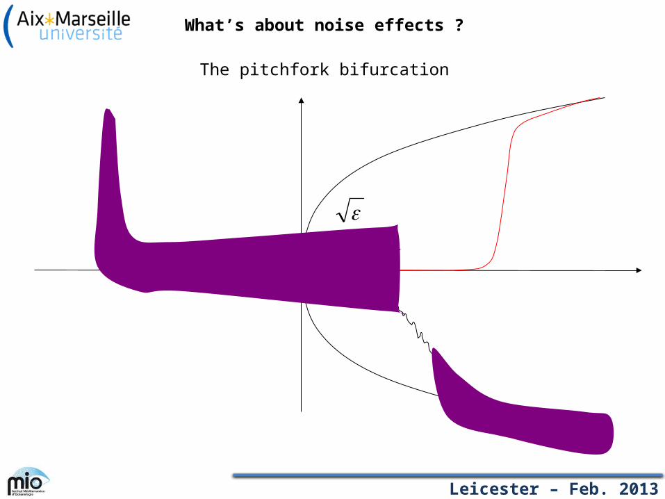
The pitchfork bifurcation

3yxyd

dyd

dx

.0 toclose timeaafter axis then thisleaves

and 0;0point theuntil axis thisfollows axis,- theto

goesy trajector then the,0)0( and 00 if :Result

x

x

yx

x

y



A general geometrical method

Dumortier and Roussarie, 1996, 2003, and now others...



A general geometrical method

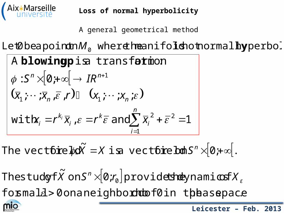
.hyperbolicnormally not is manifold the whereon point a be 0Let 0M

1 and ,with

;;;,,;;

;0:

:ation transforma is A

2

1

2

11

1

n

ii

ki

ki

nn

nn

xrxrx

xxrxx

IRS

i

up blowing

.;0on field vector a is ~

field vector The * nSXX

.space phase in the 0 of odneighborho aon 0 smallfor

of dynamics theprovides ;0on ~

ofstudy The 0

ε

n XrSX



Example

yxa

xy

dt

dyxa

xyxx

dt

dx

1

Blow up

ayv

xu

:Let

a

y

x



Example

u

v

0;0



Example

u

v

1u1v

0;0



Example

Ovrara

v

dt

vd

vrara

r

dt

dr

u

1

1

: 1chart In the

r

va1



Example

u

v y

x


What’s about noise effects?


What’s about noise effects ?

The general model

tttttt

tttttt

dWyxGdtyxgdy

dWyxFdtyxfdx

,,1

,',

0 when bounded is '

process Wiener a is 0ttW



The generic case : normal hyperbolicity

xyyyxM *;

: stableally asymptoticuniformly

manifold slow a has system the,0'for : Hypothesis

theorem.Fenichel the viaobtained manifold theLet M

time.longlly exponentia

an during in stays in enteringctory each trajesuch that of

odneighborho a exists There : 2003) Gentz, and (Berglund Theorem

BBMB



The generic case : normal hyperbolicity

0M

M

B



The saddle node bifurcation

tt

t

dWyxdy

dx

21

1



The saddle node bifurcation




tt

t

dWyxydy

dx

31

1


Conclusions

• It has recently been completed for the analysis of non normally hyperbolic manifolds

• Noise can have important effects when its various is large enough

• Various applications : Food webs models, gene networks, chemical reactors

• GSP theory provides a rigorous way to build and analyze aggregated models

• This advance permits to deal with systems having more than one aggregated model



Introduction

• Complex systems dynamics (high number of entities interacting in nonlinear way, networks, loops and feed-back loops, etc.) - Ecosystems

• Response of the complete network to a given perturbation (contamination, exploitation, global warming, …) on a particular part of the system? (amplified, damped, how and why?)

• processes intensities and variations;• the whole system dynamics;• from individuals to communities and back;

MODELLING:

• How does the formulation of a process in a complex system affect the whole system dynamics? How to measure the impacts of a perturbation?


Introduction

Individuals

Functional groups

Communities

Ecosystems

Bioenergetics – Genetic properties – Metabolism –

Physiology - Behaviours

Activities – Genetic and Metabolic expressions

Biotic interactions – Trophic webs

Environmental forcing – – Energy assessments –

Human activities

Complexity

Information - Data


Introduction

How can we used data got in laboratory experiments to field models? How can we take benefit of the large amount of data obtained at small scales to understand global system functioning?

Can we link different data sets obtained at different scales?

For a given process in a complex system, what is the effect of its mathematical formulation on the whole dynamics? Does it matter if it is well quantitatively validated?

For a given process, we often use functions even if we know that it is a bad representation, because it is simpler : is there a simple alternative?

For an given ecosystem, many models can be developed. How to choose? One of them can be valid during a given time period while another will be efficient for another period : how do we know the sequence of the models to use?


Introduction

STRUCTURE SENSITIVITY


Structure sensitivity


Sensitivity to function g ? gR : Reference model = MR

gP : Perturbed model = MP





Ref. formulation= Holling Ref. formulation= Ivlev

0 5 10 15 20 25 30 35 40 45 500

0.5

1

1.5

2

2.5

3

3.5

4

Tau

x d

’ab

sorp

tion

de

Si (

d-

1)

Concentration de Si (mmol.l-1)


Zooplancton

Phytoplancton

Nutriments



0

0.5

1

1.5

2

2.5

30

0.5

1

1.5

2

2.5

3

0

0.1

0.2

0.3

0.4

0.5

0.6

0.7

0.8

S2 concentration

S1 concentration

j S2


PROCESS FORMULATION :FUNCTIONAL RESPONSE


Functional response

Process which describes the biomass flux from a trophic level to another one : the functional response aims to describe this process at the population level.

However, it results from many individual properties :

• behavior (interference between predators, optimal foraging, ideal free distribution, etc.)

• physiology (satiation, starvation, etc.)

And population properties as well:

• population densities (density-dependence effects)

• populations distribution (encounter rates, etc.)

How should we formulate the functional response? At which scale?


Functional response

Process which describes the biomass flux from a trophic level to another one : the functional response aims to describe this process at the population level.

However, it results from many individual properties :

• behavior (interference between predators, optimal foraging, ideal free distribution, etc.)

• physiology (satiation, starvation, etc.)

And population properties as well:

• population densities (density-dependence effects)

• populations distribution (encounter rates, etc.)

How should we formulate the functional response? At which scale?

Current ecosystem models are sensitive to the functional response formulation.


Functional response

Small scale : experiments

Large scale : integrate spatial variability and individuals displacement (behavior, …)


Functional response


11 1

11

bx

axey

d

dy

ybx

ax

K

xrx

d

dx

Holling idea:

Searching Handling

Functional response


11 1

11

bx

axey

d

dy

ybx

ax

K

xrx

d

dx

Holling idea:

Searching Handling

x is assumed constant at this scale of description

Functional response


bx

axxg

1Holling type II (Disc equation – Holling 1959)

Searching Handling

x

Functional response


bx

axxg


Searching Handling

x

Functional response

or yyy

ooro

rrorr

r

yyxyd

dy

yeaxyyxyd

dy

axyxxrd

dx


bx

axxg


Searching Handling

x

ooro

rrorr

r

yyxyd

dy

yeaxyyxyd

dy

axyxxrd

dx

or yyy yx

yr

x

axxg

1

Functional response


Functional response


Functional response

2

1


Functional response


Functional response

Local Holling type II functional responses

Global Holling type III functional response

<0

>0

=> Conditions can be found to get the criterion for Holling Type III functional responses


Dynamical consequences

1 – On each patch separately, the parameter values are such that periodic solutions occur.

2 – With density-dependent migration rates of the predator satisfying the above mentioned criterion for Holling Type III functional response, the system is stabilized

3 – With constant migration rates, taking extreme values observed in the situation described in 2, the system exhibits periodic fluctuations : the stabilization results from the change of functional response type.



• Global type III FR can emerge from local type II functional responses associated to density-dependent displacements

• The Holling Type III functional response leads to stabilization

• The stability actually results from the type (type II functional responses lead to periodic fluctuations even if they are quantitatively close to the type III FR)

• The Type III results from density-dependence : the effect of density-dependent migration rates on the global functional response can be understood explicitely.



Functional response in the field : a set of functions instead of one function?

• Shifts between models

• Multi-stability of the fast dynamics

• Changes of fast attractors : bifurcation in the fast part of the system induced by the slow dynamics

• We use functions to represent FR at a global scale even if we know that it is a bad representation, because it is simpler : is there a simple alternative?


SHIFTS BETWEEN MODELS : LOSS OF NORMAL HYPERBOLICITY


Slow-Fast vector fields

yxgd

dy

yxfd

dx

,

,

0

0,,

y

yxfx

yxx * Top – down

,,

,,

yxgy

yxfx

,,,,

,*

*

yGyyxgy

yxx

Bottom – up


Fenichel theorem (Geometrical Singular Perturbation Theory)


• The jump between two formulations can be described by the Geometrical Singular Perturbation Theory : follow the trajectories of the full system around the points where normal hyperbolicity is lost («Blow up techniques »)

Conclusions (2/2)

• Instead of one function to formulate one process at large scale, several functions can be used.

• Multiple equilibria in the fast dynamics can provide a mechanism for this multiple representation in large scale models.

• Bifurcations of the fast dynamics induced by slow dynamics lead to shifts in the fast variables. This leads to several mathematical expressions of the fast equilibrium with respect to slow variables : each of them provides a mathematical formulation at large scales


Thanks to my collaborators…

Roger ARDITI

Julien ARINO

Ovide ARINO

Pierre AUGER

Rafael BRAVO de la PARRA

François CARLOTTI

Flora CORDOLEANI

Marie EICHINGER

Frédérique FRANCOIS

Mathias GAUDUCHON

Franck GILBERT

Bas KOOIJMAN

Bob KOOI

Horst MALCHOW

Claude MANTE

Marcos MARVA

Andrei MOROZOV

David NERINI

Tri NGUYEN HUU

Robert ROUSSARIE

Eva SANCHEZ

Richard SEMPERE

Georges STORA

Caroline TOLLA

… and thanks for your attention!Leicester – Feb. 2013

jean-christophe poggiale aix-marseille université mediterranean institute of oceanography u.m.r....

Documents