Jens Vygen

New approximation algorithms for the TSP

The traveling salesman problem (TSP) is probably the best known combinatorial optimiza-tion problem. Although studied intensively for sixty years, the TSP continues to pose grandchallenges. Cook’s [2012] recent book gives an excellent introduction.

Since the TSP is NP-hard (Karp [1972]), it is natural to ask for approximation algorithms.How good solutions can we guarantee to find in polynomial time? Christofides [1976] deviseda 3

2 -approximation algorithm for the Symmetric TSP: it always finds a solution that is atmost 50% longer than optimum.

Can we do better? Can we do similarly well for the Asymmetric TSP? These questions– still unsolved – belong to the most intriguing open problems in our field. Recently, there hasbeen progress that makes us hope that we will learn more in the near future.

In this survey we try to describe the state of the art, in particular the recent progress, mostlyfrom 2010–2012. We use standard notation and some basic terminology and well-known resultsfrom combinatorial optimization; see Korte and Vygen [2012] or Schrijver [2003] if necessary.

1 IntroductionLet us first review different formulations of the problems and basic approximation algorithms.

1.1 Asymmetric TSP and Symmetric TSPThe Asymmetric TSP can be defined as follows. Given a finite set V (of cities) and distancesc(v, w) ≥ 0 for all v, w ∈ V (also called length or cost), find a closed walk of minimum totallength visiting each city at least once. More precisely, we look for a sequence v0, v1, . . . , vk withvk = v0 and v0, . . . , vk = V (also called a tour) such that

∑ki=1 c(vi−1, vi) is minimum.

The Symmetric TSP is the special case in which the distances are symmetric: c(v, w) =c(w, v) for all v, w ∈ V .

Often these problems are formulated such that each city must be visited exactly once insteadof at least once (except, of course, that we must end in the same city where we start). This isequivalent if the distances obey the triangle inequality

c(u,w) ≤ c(u, v) + c(v, w) for all u, v, w ∈ V (1)

because then we can shortcut whenever we visit a city a second time.On the other hand, given an instance of the Asymmetric TSP (or Symmetric TSP) as

defined above, we can set

c(v, w) := min∑

e∈E(P ) c(e) : P path from v to w, V (P ) ⊆ V

and consider (V, c) instead. Note that c obeys (1). The instance (V, c) is equivalent to (V, c)because we can move from v to w at cost c(v, w) via a shortest v-w-path. The pair (V, c) iscalled the metric closure of (V, c).

2

1.2 Approximation algorithmsA ρ-approximation algorithm (for a minimization problem) is an algorithm that runs in poly-nomial time and always computes a solution (here: a tour) that costs at most ρ times theoptimum. Here ρ can be a constant or a function of n; here and henceforth n = |V | denotesthe number of cities.

If we do not require the triangle inequality but still want to visit every city exactly once, theproblems look hopeless: any approximation algorithm would allow us to decide in polynomialtime whether a given graph contains a Hamiltonian circuit, and thus imply P = NP (this easyobservation is due to Sahni and Gonzalez [1976]).

So we assume henceforth that we may visit cities more than once.

1.3 Euler’s theoremFor the total length of a tour, all that matters is how many times we move from v to w foreach ordered pair (v, w), or how many times we move between v and w for each unorderedpair v, w in the undirected case. Hence we can represent a tour by a directed or undirectedgraph (possibly with parallel edges) with vertex set V . As observed by Euler [1736], this graphhas two properties:(a) it is connected;and for every city:(b′) the in-degree equals the out-degree in the directed case;(b′′) the degree is even in the undirected case.

Digraphs with the properties (a) and (b′) and undirected graphs with properties (a) and (b′′)are called Eulerian. The conditions are equivalent to the existence of an Eulerian walk : a closedwalk traversing every edge exactly once and every vertex at least once. Given an Eulerian graphor digraph, one can find an Eulerian walk in linear time (Hierholzer [1873]).

Therefore, one can reformulate the Asymmetric TSP and the Symmetric TSP by askingfor a (multi)set F such that (V, F ) is an Eulerian (directed or undirected, respectively) graphwith minimum total length c(F ). We call such an F a tour, too. Here and in the following weabbreviate c(F ) :=

∑e∈F c(e) and c(e) := c(v, w) for any edge e from v to w.

1.4 Graphic TSPA natural special case of the Symmetric TSP arises when we are given a connected undirectedgraph G and let V = V (G) and c(v, w) = 1 if v, w ∈ E(G) and c(v, w) = ∞ otherwise.This problem is called the Graphic TSP. The metric closure (V, c) of (V, c) is also called themetric closure of G. Functions c arising in this way are called graphic metrics.

By the observations in Section 1.3, the Graphic TSP can be reformulated as follows.Given a connected graph G, find an Eulerian spanning multi-subgraph (V, F ) with minimum|F |. Here a multi-subgraph arises from a subgraph by doubling a subset of its edges. Again,we call an Eulerian multi-subgraph of G simply a tour in G.

The Graphic TSP has also been called Graph TSP by some authors. It is easy to seethat, without loss of generality, we may assume that G is 2-vertex-connected (otherwise find atour in each block separately).

3

1.5 Double tree and Christofides’ algorithmA 2-approximation algorithm for the Symmetric TSP is easy: take a tree on vertex set Vwith minimum total edge length (it is well-known that such a minimum spanning tree can befound efficiently, e.g., by the greedy algorithm), and double all its edges. Since any tour isconnected and thus contains a spanning tree, a minimum spanning tree cannot be longer thanan optimum tour. Hence we have a 2-approximation algorithm.

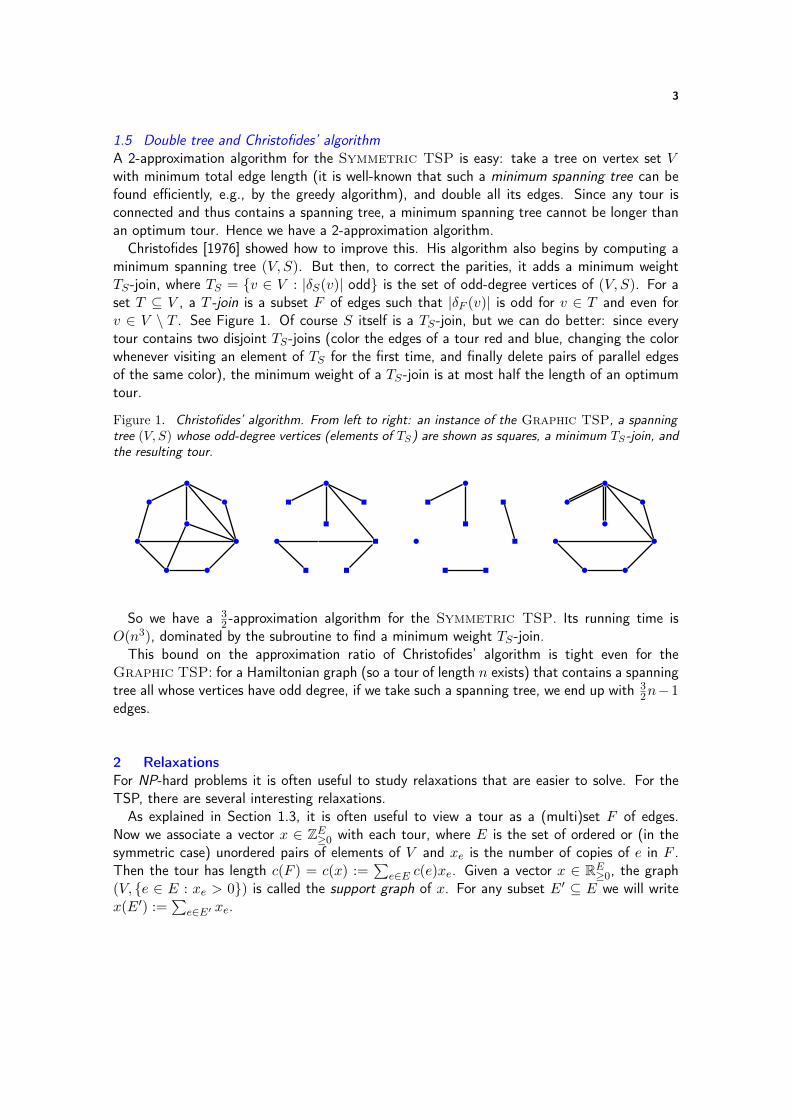
Christofides [1976] showed how to improve this. His algorithm also begins by computing aminimum spanning tree (V, S). But then, to correct the parities, it adds a minimum weightTS-join, where TS = v ∈ V : |δS(v)| odd is the set of odd-degree vertices of (V, S). For aset T ⊆ V , a T -join is a subset F of edges such that |δF (v)| is odd for v ∈ T and even forv ∈ V \ T . See Figure 1. Of course S itself is a TS-join, but we can do better: since everytour contains two disjoint TS-joins (color the edges of a tour red and blue, changing the colorwhenever visiting an element of TS for the first time, and finally delete pairs of parallel edgesof the same color), the minimum weight of a TS-join is at most half the length of an optimumtour.

Figure 1. Christofides’ algorithm. From left to right: an instance of the Graphic TSP, a spanningtree (V, S) whose odd-degree vertices (elements of TS) are shown as squares, a minimum TS-join, andthe resulting tour.

So we have a 32 -approximation algorithm for the Symmetric TSP. Its running time is

O(n3), dominated by the subroutine to find a minimum weight TS-join.This bound on the approximation ratio of Christofides’ algorithm is tight even for the

Graphic TSP: for a Hamiltonian graph (so a tour of length n exists) that contains a spanningtree all whose vertices have odd degree, if we take such a spanning tree, we end up with 3

2n−1edges.

2 RelaxationsFor NP-hard problems it is often useful to study relaxations that are easier to solve. For theTSP, there are several interesting relaxations.

As explained in Section 1.3, it is often useful to view a tour as a (multi)set F of edges.Now we associate a vector x ∈ ZE≥0 with each tour, where E is the set of ordered or (in thesymmetric case) unordered pairs of elements of V and xe is the number of copies of e in F .Then the tour has length c(F ) = c(x) :=

∑e∈E c(e)xe. Given a vector x ∈ RE≥0, the graph

(V, e ∈ E : xe > 0) is called the support graph of x. For any subset E′ ⊆ E we will writex(E′) :=

∑e∈E′ xe.

4

2.1 Subtour LPLet (V, c) be an instance of the Symmetric TSP, n = |V | ≥ 3, and E =

(V2

). The following

LP, first formulated by Dantzig, Fulkerson and Johnson [1954], has often been called subtourelimination LP or simply subtour LP or Held-Karp relaxation:

min c(x)

subject to x(δ(U)) ≥ 2 (∅ 6= U ⊂ V )x(δ(v)) = 2 (v ∈ V )

xe ≤ 1 (e ∈ E)xe ≥ 0 (e ∈ E)

(2)

Note that the constraints xe ≤ 1 (e ∈ E) could be omitted as they are implied by the otherconstraints: for e = u, v we have 2xe = x(δ(u)) + x(δ(v))− x(δ(u, v)) ≤ 2 + 2− 2.

The set of feasible solutions of the subtour LP (2) is called the subtour polytope. The integralfeasible solutions of (2) are exactly the incidence vectors of Hamiltonian circuits. Their convexhull is called the TSP polytope.

So (2) is a relaxation of the Symmetric TSP if the triangle inequality holds. For a generalinstance, we can consider (2) for its metric closure.

This relaxation has been tightened by many classes of additional valid inequalities. It isalso the basis of branch-and-cut algorithms (with exponential worst-case running time) thatmade impressive progress over the last four decades and have found optimum solutions to TSPinstances with up to 85 900 cities; see Applegate et al. [2006].

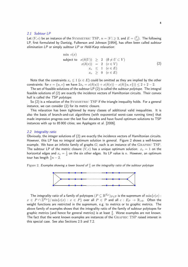
2.2 Integrality ratioObviously, the integer solutions of (2) are exactly the incidence vectors of Hamiltonian circuits.However, this LP has no integral optimum solution in general. Figure 2 shows a well-knownexample. We have an infinite family of graphs G; each is an instance of the Graphic TSP.The subtour LP of the metric closure (V, c) has a unique optimum solution: xe = 1 on thehorizontal edges and xe = 1

2 on the six other edges. Its LP value is n. However, an optimumtour has length 4

3n− 2.

Figure 2. Examples showing a lower bound of 43 on the integrality ratio of the subtour polytope

The integrality ratio of a family of polytopes (P ⊆ REP )P∈P is the supremum of minc(x) :x ∈ P ∩ ZEP /minc(x) : x ∈ P over all P ∈ P and all c : EP → R>0. Often theweight functions are restricted in the supremum, e.g. to metrics or to graphic metrics. Theabove family of examples shows that the integrality ratio of the family of subtour polytopes forgraphic metrics (and hence for general metrics) is at least 4

3 . Worse examples are not known.The fact that the worst known examples are instances of the Graphic TSP raised interest inthis special case. See also Sections 2.5 and 7.2.

5

2.3 Spanning treesThe difficulty of the Symmetric TSP lies in the combination of connectivity and parityrequirements. If we require only connectivity, a minimum spanning tree does the job. Edmonds[1970] gave the following polyhedral description:

Proposition 1. The convex hull of incidence vectors of trees with vertex set V and edges inE is the set of vectors x ∈ RE with

x(E) = n− 1∑e=v,w∈E:v,w∈U xe ≤ |U | − 1 (∅ 6= U ⊂ V )

xe ≥ 0 (e ∈ E)

(3)

This set is called the spanning tree polytope of the graph (V,E). The following easy obser-vation was made by Asadpour et al. [2010], strengthening a result of Held and Karp [1970]:

Proposition 2. If x is a feasible solution of (2), then n−1n x is in the relative interior of the

spanning tree polytope of the support graph.

Proof. We have n−1n x(E) = n−1

2n

∑v∈V x(δ(v)) = n−1 as well as

∑e=v,w∈E:v,w∈U

n−1n xe =

n−12n (

∑v∈U x(δ(v))−x(δ(U))) = n−1

2n (2|U |−x(δ(U))) ≤ n−1n (|U |−1) for any ∅ 6= U ⊂ V .

2.4 T -joinsNow consider the parity aspect. Edmonds and Johnson [1973] proved:

Proposition 3. The minimum weight of a T -join in a graph (V,E) with weights c ∈ RE≥0 andT ⊆ V equals the optimum value of the LP:

min c(x)

subject to x(δ(U)) ≥ 1 (U ⊆ V, |U ∩ T | odd)xe ≥ 0 (e ∈ E)

(4)

The cuts δ(U) with |U ∩ T | odd are called T -cuts.For negative weights the LP (4) cannot be used directly. We will also need:

Proposition 4. The convex hull of incidence vectors of T -joins in (V,E) is the set of vectorsx ∈ [0, 1]E with

|F | − x(F ) + x(δ(U) \ F ) ≥ 1 (U ⊆ V, F ⊆ δ(U),|U ∩ T |+ |F | odd)

(5)

This is called the T -join polytope of (V,E). A minimum weight T -join can be found inO(n3) time via weighted matching. See Schrijver [2003] or Korte and Vygen [2012] for detailsand proofs of Propositions 1, 3, and 4.

2.5 Wolsey’s analysisWolsey [1980] proved that Christofides’ algorithm computes a tour of length at most 3

2L, whereL is the LP value of (2). In fact, this is easy to see from the above: By Proposition 2, theminimum weight of a spanning tree is at most L. By Proposition 3, the minimum weight of aT -join is at most L

2 for any T ⊆ V with |V | even.This shows that the integrality ratio of (2) is at most 3

2 . No better upper bound is known ingeneral.

6

2.6 Two-edge-connected spanning subgraphsEvery tour is 2-edge-connected, so a relaxation of the Symmetric TSP is to find a minimumweight 2-edge-connected spanning subgraph (if the triangle inequality holds) or multi-subgraph.Unfortunately, these problems are also NP-hard (cf. Section 7.6).

Let G = (V,E) be a 2-edge-connected undirected graph. Then the incidence vectors of the2-edge-connected spanning subgraphs (2ECSS) of G are the integral feasible solutions of thefollowing LP:

min c(x)

subject to x(δ(U)) ≥ 2 (∅ 6= U ⊂ V )xe ≤ 1 (e ∈ E)xe ≥ 0 (e ∈ E)

(6)

This LP arises from (2) by omitting the equality constraints. If we allow using edges twice, theLP (6) can be simplified further by omitting the upper bounds:

min c(x)

subject to x(δ(U)) ≥ 2 (∅ 6= U ⊂ V )xe ≥ 0 (e ∈ E)

(7)

Cunningham (see Monma, Munson and Pulleyblank [1990]) and Goemans and Bertsimas[1993] observed:

Proposition 5. If (V,E) is a complete graph, |V | ≥ 3, and c obeys the triangle inequality,then the optimum values of (2), (6), and (7) are the same.

Proof. Let x be a rational feasible solution of (7). Choose k ∈ N such that kxe is an eveninteger for each e ∈ E. If there is a vertex v ∈ V with x(δ(v)) > 2, choose incidentedges e = v, w and e′ = v, w′ with xe > 0 and xe′ > 0, reduce xe and xe′ each by 1

kand increase xw,w′ by 1

k while maintaining feasibility (the existence of two such edges e, e′

follows from applying Lovász’ [1976] splitting theorem to the Eulerian graph with kxe copiesof each edge e). Note that we maintain the property that kx(δ(v)) is an even integer for allv ∈ V , so we end up with a feasible solution of (7) also satisfying x(δ(v)) = 2 for all v ∈ V .Then also xe = 1

2(x(δ(v)) + x(δ(w)) − x(δ(v, w))) = 12(2 + 2 − x(δ(v, w))) ≤ 1 for all

e = v, w ∈ E, so we have a feasible solution of (2). Due to the triangle inequality we neverincreased c(x).

We also note:

Proposition 6. If (V,E) is a 2-edge-connected graph and c(e) = 1 for all e ∈ E, then theoptimum values of (6) and (7) are the same.

Proof. Let x be an optimum solution of (7). Let f = v, w ∈ E with xf > 1. Call twovertices a and b close if x(δ(a ∪ S) \ f) ≥ 1 for all S ⊆ V \ a, b. This is a transitiverelation. If v and w are close, then we can reduce xf to 1 and maintain feasibility. Otherwiseeach vertex is either close to v or close to w; so there is an edge f ′ = v′, w′ such that v andv′ are close, w and w′ are close, and xf ′ < 1. Then increasing xf ′ to min1, xf ′ + xf − 1and decreasing xf to 1 maintains feasibility.

7

The same holds for integral solutions: we never need to take two copies of any edge, exceptof course for bridges of G.

The constraints of (7) define facets of the graphical traveling salesman polyhedron: theconvex hull of vectors x ∈ ZE≥0 for which x(δ(U)) ∈ 2, 4, 6, . . . for all ∅ 6= U ⊂ V . This wasstudied by Cornuéjols, Fonlupt and Naddef [1985].

2.7 Asymmetric subtour LPLet (V, c) be an instance of the Asymmetric TSP with (1) and E = (v, w) : v, w ∈ V, v 6=w. The following is the natural analogon of the subtour LP in this case:

min c(y)

subject to y(δ+(U)) ≥ 1 (∅ 6= U ⊂ V )y(δ+(v)) = y(δ−(v)) = 1 (v ∈ V )

ye ≥ 0 (e ∈ E)

(8)

Again, the integral feasible solutions to this LP are exactly the Hamiltonian circuits. Vectorsy ∈ RE≥0 with y(δ+(v)) = y(δ−(v)) for all v ∈ V are called circulations in (V,E).

From a feasible solution y to (8) one can obtain a feasible solution to (2) by setting xv,w :=

y(v,w) + y(w,v) for all v, w ∈(V2

).

2.8 Solving the linear programsAll linear programs above have exponentially many constraints, but they can all be solved inpolynomial time; in fact an optimum basic solution can be found in polynomial time. One wayto show this is via the equivalence of optimization and separation. The LPs for spanning treesand T -joins can be solved by combinatorial algorithms. For the LPs (2), (6), (7), and (8),there are straightforward polynomial-size extended formulations (by introducing flow variablesand using the max-flow min-cut theorem), but combinatorial algorithms to solve these LPs arenot known. Held and Karp [1970], however, showed how to solve (2) fast approximately.

2.9 Optimum basic solutionsAny optimum basic solution x∗ of any of the LPs (2), (6), and (7) has at most 2n− 3 nonzerovariables; in fact the subgraph of the support graph induced by U has at most 2|U | − 3 edgesfor any U ⊆ V with |U | ≥ 2 (cf. Cornuéjols, Fonlupt and Naddef [1985] and Goemans [2006]).

Any optimum basic solution x∗ of the LP (8) has at most 3n− 4 nonzero variables (and thesubgraph of the support graph induced by U has at most 3|U | − 4 edges for any U ⊆ V with|U | ≥ 2); this was also shown by Goemans [2006].

The basic feasible solutions of (8) arise as the unique solutions of a linear equation systemwith all coefficients 0 or 1, so by Cramer’s rule each of their components can be written as a

b forintegers a and b ≤ (3n−4)!/2. The same holds for (2), (6), and (7), even with b ≤ (2n−3)!/2.

2.10 Covering the cities by disjoint circuitsAnother relaxation works both in the directed and undirected case. We ignore connectivityand look for a graph in which each city belongs to a circuit and the circuits are pairwisevertex-disjoint.

In the undirected case, such an edge set is called a perfect 2-matching because every vertexmust have degree 2. A minimum weight perfect 2-matching can be found in polynomial time

8

(this is essentially equivalent to nonbipartite weighted matching), but it did not prove useful inthe design of approximation algorithms so far.

In the directed case, the analogous relaxation is even easier to solve. Here every vertex musthave in-degree and out-degree 1. A minimum weight spanning subgraph with this property caneasily be found by solving a bipartite weighted matching problem. This was used for the firstnontrivial approximation algorithm for the Asymmetric TSP, to be described next.

2.11 O(log n)-approximation for Asymmetric TSPFor the Asymmetric TSP no constant-factor approximation algorithm is known, so we willconsider f(n)-approximation algorithms, where f(n) is a function of the number n of cities. Itis trivial to give an n-approximation algorithm: order the cities arbitrarily, say V = v1, . . . , vn,and take a shortest vn-v1-path and a shortest vi−1-vi-path for i = 2, . . . , n.

The first nontrivial approximation algorithm was found by Frieze, Galbiati and Maffioli [1982].It assumes that the triangle inequality holds and works as follows.

Begin with W := V . Find a minimum weight subset F of edges with |δ+F (v)| = |δ−F (v)| = 1

for all v ∈ W and |δ+F (v)| = |δ−F (v)| = 0 for all v ∈ V \W (cf. Section 2.10). Then pick one

vertex from each connected component of (W,F ), and replace W by the set of these vertices.Iterate until (W,F ) is connected.

The set of all edges chosen in this algorithm forms an Eulerian graph. Due to the triangleinequality, the total cost of edges picked in each iteration is at most the length of an optimumtour. Since |W | decreases by a factor of two in each iteration, we are done after blog2 nciterations. Hence we have a (log2 n)-approximation algorithm.

Bläser [2003], Kaplan et al. [2005], and Feige and Singh [2007] improved this by a constantfactor.

3 Random samplingIt is quite natural to first take a spanning tree to guarantee connectivity, and then add a mini-mum cost set of edges in order to make the graph Eulerian. This idea (underlying Christofides’algorithm) works also in the directed case as we shall see soon (in the proof of Theorem 8).

A minimum spanning tree does often not give the best overall result. A certain kind ofrandom sampling led to better approximation algorithms for the Asymmetric TSP and theGraphic TSP.

3.1 Thin treesAsadpour, Goemans, Mądry, Oveis Gharan and Saberi [2010] were the first to obtain an o(log n)-approximation algorithm for the Asymmetric TSP. Their algorithm is randomized. The mainingredient is the following result, which, interestingly, applies to an undirected instance:

Theorem 7. There is a randomized polynomial-time algorithm which, given a feasible solutionx of the LP (2), computes a spanning tree (V, S) such that with probability at least 1

2 we havec(S) ≤ 2c(x) and |δS(U)| ≤ αx(δ(U)) for all U ⊆ V , where α = 4 log n/ log log n.

The last property is called α-thinness. By Proposition 2, n−1n x is a convex combination of

spanning trees, i.e. n−1n xe =

∑S∈S:e∈S pS for all e ∈ E, where S is the set of (edge sets of)

spanning trees, pS ≥ 0 for all S ∈ S and∑

S∈S pS = 1. Such an explicit convex combinationcan be obtained in polynomial time. If we pick each tree S ∈ S with probability pS , the

9

expected cost is∑

e∈E c(e)xe, and hence the cost at most is twice as much with probability atleast 1

2 .The difficulty is that such a random spanning tree will in general not be thin enough. There-

fore Asadpour et al. [2010] choose the probability distribution carefully, namely such that itmaximizes the entropy

∑S∈S pS log 1

pS. Equivalently, pS = γΠe∈Sλe for all S ∈ S, for suitable

positive numbers γ and λe (e ∈ E). Such a distribution is also called λ-uniform.Asadpour et al. [2010] show how to sample trees efficiently from approximately this distri-

bution. Moreover, they prove that the random variables indicating for each edge whether it ispart of the selected tree are negatively correlated; then thinness is implied by a Chernoff boundtogether with the fact that in any graph there are less than 2n2γ many γ-approximate mini-mum cuts, for any γ ≥ 1 (Karger and Stein [1996]). See Asadpour et al. [2010] for the details.(Alternatively, a thin tree can be obtained by the dependent randomized rounding approach ofChekuri, Vondrák and Zenklusen [2010].)

3.2 The O(log n/ log logn)-approximation algorithmUsing Theorem 7, the randomized O(log n/ log log n)-approximation algorithm of Asadpour etal. [2010] and its analysis can be described easily. We work in the metric closure, so c satisfiesthe triangle inequality.

First solve the LP relaxation (8) to obtain a vector y. Then get a solution x of (2) by settingxv,w := y(v,w) + y(w,v) for all v, w ∈

(V2

). Note that xe = 0 or xe ≥ 1

(3n−4)! for all e ∈(V2

)(cf. Section 2.9); so x can be stored with O(n2 log n) bits.

Next apply Theorem 7 to obtain a spanning tree (V, S). Orient the edges of this tree byreplacing each v, w ∈ S by the cheaper one of (v, w) and (w, v). Setting c′(v, w) :=minc(v, w), c(w, v), we get with probability at least 1

2 that the resulting arc set R satisfiesc(R) = c′(S) ≤ 2c′(x) ≤ 2c(y) as well as |δ−R(U)| ≤ |δS(U)| ≤ αx(δ(U)) = α(y(δ−(U)) +y(δ+(U))) = 2αy(δ+(U)) for all U ⊆ V .

Finally apply the following Theorem 8 to R and y. With probability at least 12 we obtain a

tour of length at most (2α+ 2)c(y).

Theorem 8. Let (V,R) be a connected spanning subgraph of the complete digraph (V,E),y ∈ RE≥0, and β > 0 such that |δ−R(U)| ≤ βy(δ+(U)) for all U ⊆ V (G). Then we can find atour F with c(F ) ≤ c(R) + βc(y) in polynomial time.

Proof. Let l(e) := 1 for e ∈ R and l(e) := 0 for e ∈ E \ R. Any integral circulation f in(V,E) with f ≥ l corresponds to a tour. We compute an integral minimum cost circulationf∗ ≥ l and note that the resulting tour has cost c(f∗).

To prove that such a circulation (and hence an integral circulation) of cost at most c(R) +βc(y) exists, we let u(e) := maxl(e), βye for all e ∈ E and observe that a circulation g withl ≤ g ≤ u exists; then c(f∗) ≤ c(g) ≤

∑e∈E c(e)u(e) ≤ c(R) + βc(y).

The existence of g follows from Hoffman’s [1960] circulation theorem: we have l ≤ u andl(δ−(U)) = |δ−R(U)| ≤ βy(δ+(U)) ≤ u(δ+(U)) for all U ⊆ V .

3.3 Random sampling for the Symmetric TSPThe random sampling of Asadpour et al. [2010] was also used by Oveis Gharan, Saberi andSingh [2011] for the first improvement over Christofides’ algorithm for the Graphic TSP.

They proposed the following algorithm. Take the metric closure and solve the subtour LP(2) to obtain an optimum basic solution x. Again, n−1

n x is a convex combination of spanning

10

trees, and we pick one at random according to a maximum entropy distribution; call it (V, S).Let TS be again the set of odd degree vertices of (V, S). Finally add a minimum-weight TS-jointo S as in Christofides’ algorithm.

Oveis Gharan, Saberi and Singh [2011] conjectured that this algorithm has better approx-imation ratio than 3

2 , but they could prove this only for the Graphic TSP, and only for aslight variant of this algorithm. Their main structure theorem is the following. (The constantsbelow are not best possible, but the improvement is tiny anyway.)

Theorem 9. Let (V, c) be an instance of the Symmetric TSP satisfying the triangle in-equality. Let x be an optimum solution of (2), and let (V, S) be a spanning tree picked atrandom according to the maximum entropy distribution (pS)S∈S with

∑S∈S:e∈S pS = n−1

n xefor all e ∈ E. Let TS be the set of odd degree vertices of (V, S). Call an edge e good if e doesnot belong to any TS-cut δ(U) with x(δ(U)) ≤ 2 + 10−15. Then at least one of the followingholds:(a) there is a subset E∗ of edges with x(E∗) ≥ 10−12n such that for each e ∈ E∗ the

probability that e is good is at least 10−24;(b) there are at least 19

20n edges e with xe ≥ 1− 10−7.

The proof of this theorem is very long. It uses deeper results about random spanning treesand the structure of near-minimum cuts.

3.4 First improvement over Christofides for the Graphic TSPFollowing Oveis Gharan, Saberi and Singh [2011], we show now that Theorem 9 implies a betterapproximation ratio for the Graphic TSP.

In case (a), Wolsey’s analysis can be improved: let ye := xe/(2 + 10−15) for good edgese and ye := xe/2 for other edges e. Since y(δ(U)) ≥ 1 for every TS-cut δ(U), we concludethat y is a feasible solution to (4). Therefore the expected cost of a minimum weight TS-join is at most c(y) ≤ 1

2c(x) − 10−16∑

e∈E:e good c(e)xe ≤12c(x) − 10−40

∑e∈E∗ c(e)xe.

If c is a graphic metric, we have c(e) ≥ 1 for all e ∈ E and c(x) ≤ 2n. Then we getc(y) ≤ 1

2c(x)− 10−40x(E∗) ≤ 12c(x)− 10−52n ≤ 1

2(1− 10−52)c(x).In case (b), the approximation ratio is better, and the proof is also easy. Let I be the set of

edges e with xe ≥ 1− 10−7. The edges in I form vertex-disjoint paths and circuits, and eachcircuit has length at least 107 (or is Hamiltonian). Remove one edge from each circuit and addedges of cost 1 to obtain a spanning tree (V, S). Note that c(S \I) = |S \I| < ( 1

20 +10−7)n ≤( 1

20 +10−7)c(x). We get c(S) = c(S∩I)+c(S\I) ≤∑

e∈S c(e)xe/(1−10−7)+( 120 +10−7)c(x).

Finally we add a minimum weight TS-join J , where TS is the set of vertices with odd degreein (V, S). To bound c(J), let ye := 1

3 for e ∈ S and ye := 23xe for other edges e. We show

that y is a feasible solution to (4).For any set U with |U ∩TS | odd we have |δ(U)∩S| odd. If |δ(U)∩S| = 1, then y(δ(U)) ≥

13 + y(δ(U) \ S) ≥ 1

3 + 23(x(δ(U))− 1) ≥ 1. If |δ(U) ∩ S| ≥ 3, then y(δ(U)) ≥ 3 · 1

3 = 1.Hence c(J) ≤ c(y) = 1

3c(S) + 23

∑e∈E\S c(e)xe. We conclude c(S

.∪ J) ≤ 4

3c(S) +23

∑e∈E\S c(e)xe ≤

43c(x)/(1− 10−7) + 4

3( 120 + 10−7)c(x) ≤ (7

5 + 10−6)c(x).Note that we used properties of the Graphic TSP in both cases, (a) and (b). Although

the improvement over Christofides’ algorithm is tiny (in case (a)), this result received a lot ofinterest.

11

4 Correcting parity by adding and removing edgesSo far, all algorithms began with a spanning tree and then added edges to make the graphEulerian. Mömke and Svensson [2011] had a brilliant idea: if we begin with a 2-connectedgraph, we may also delete some edges for making it Eulerian, and this may be cheaper overall.

4.1 Removable pairingsThe following definition of Mömke and Svensson [2011] is very interesting. A removable pairingin a 2-vertex-connected graph (V,E) is a pair (R,P) with the following properties:(a) R ⊆ E;(b) for each P ∈ P there exists a vertex v ∈ V and three distinct edges e1, e2, e3 incident to

v such that P = e1, e2;(c) the elements of P are pairwise disjoint;(d) for any set F ⊆ R with |F ∩ P | ≤ 1 for all P ∈ P, the graph (V,E \ F ) is connected.Mömke and Svensson [2011] proposed to obtain a removable pairing as follows.

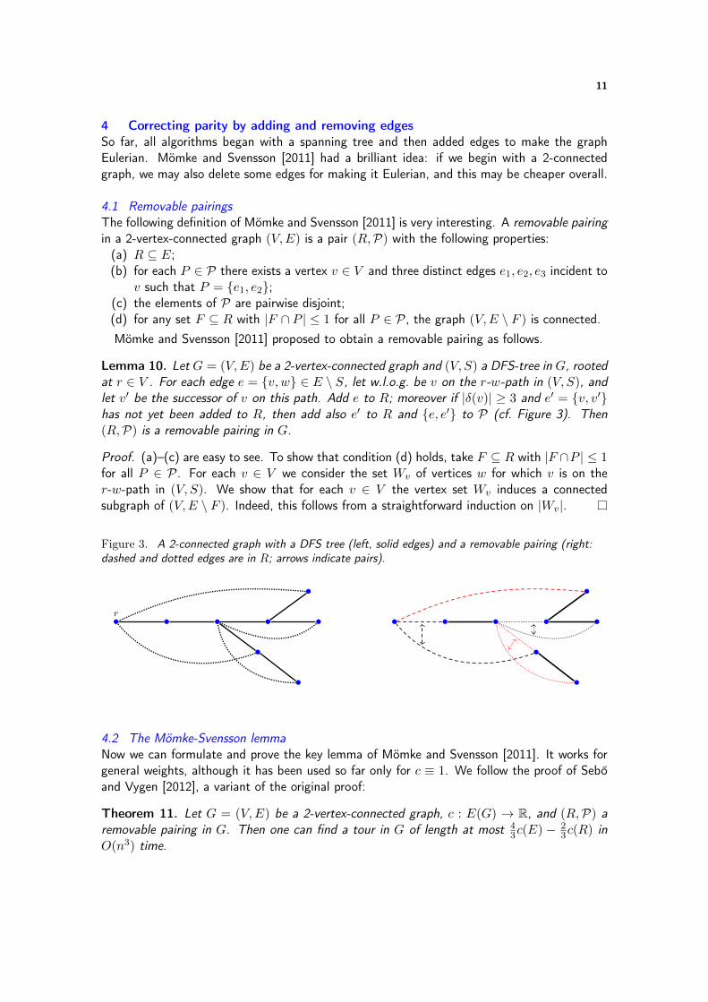
Lemma 10. Let G = (V,E) be a 2-vertex-connected graph and (V, S) a DFS-tree in G, rootedat r ∈ V . For each edge e = v, w ∈ E \ S, let w.l.o.g. be v on the r-w-path in (V, S), andlet v′ be the successor of v on this path. Add e to R; moreover if |δ(v)| ≥ 3 and e′ = v, v′has not yet been added to R, then add also e′ to R and e, e′ to P (cf. Figure 3). Then(R,P) is a removable pairing in G.

Proof. (a)–(c) are easy to see. To show that condition (d) holds, take F ⊆ R with |F ∩P | ≤ 1for all P ∈ P. For each v ∈ V we consider the set Wv of vertices w for which v is on ther-w-path in (V, S). We show that for each v ∈ V the vertex set Wv induces a connectedsubgraph of (V,E \ F ). Indeed, this follows from a straightforward induction on |Wv|.

Figure 3. A 2-connected graph with a DFS tree (left, solid edges) and a removable pairing (right:dashed and dotted edges are in R; arrows indicate pairs).

r

4.2 The Mömke-Svensson lemmaNow we can formulate and prove the key lemma of Mömke and Svensson [2011]. It works forgeneral weights, although it has been used so far only for c ≡ 1. We follow the proof of Sebőand Vygen [2012], a variant of the original proof:

Theorem 11. Let G = (V,E) be a 2-vertex-connected graph, c : E(G) → R, and (R,P) aremovable pairing in G. Then one can find a tour in G of length at most 4

3c(E) − 23c(R) in

O(n3) time.

12

Proof. Let TG be the set of odd degree vertices of G. Let c′(e) = c(e) for e ∈ E \ R andc′(e) = −c(e) for e ∈ R. For any TG-join J in G that intersects each pair P ∈ P in at mostone edge, we construct a tour from E by doubling the edges in J \ R and deleting the edgesin J ∩R. This tour has length c(E) + c′(J).

To compute a TG-join of weight at most 13c(E) − 2

3c(R) = 13c′(E), intersecting each pair

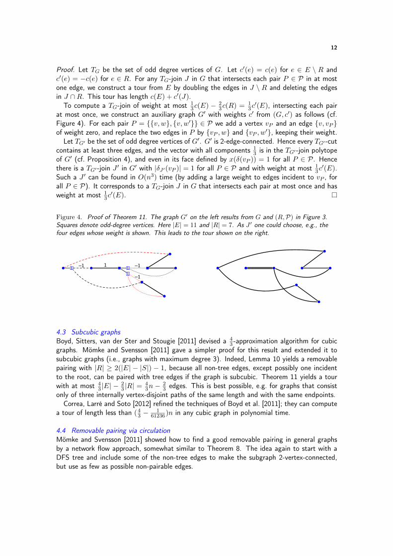
at most once, we construct an auxiliary graph G′ with weights c′ from (G, c′) as follows (cf.Figure 4). For each pair P = v, w, v, w′ ∈ P we add a vertex vP and an edge v, vP of weight zero, and replace the two edges in P by vP , w and vP , w′, keeping their weight.

Let TG′ be the set of odd degree vertices of G′. G′ is 2-edge-connected. Hence every TG′-cutcontains at least three edges, and the vector with all components 1

3 is in the TG′-join polytopeof G′ (cf. Proposition 4), and even in its face defined by x(δ(vP )) = 1 for all P ∈ P. Hencethere is a TG′-join J ′ in G′ with |δJ ′(vP )| = 1 for all P ∈ P and with weight at most 1

3c′(E).

Such a J ′ can be found in O(n3) time (by adding a large weight to edges incident to vP , forall P ∈ P). It corresponds to a TG-join J in G that intersects each pair at most once and hasweight at most 1

3c′(E).

Figure 4. Proof of Theorem 11. The graph G′ on the left results from G and (R,P) in Figure 3.Squares denote odd-degree vertices. Here |E| = 11 and |R| = 7. As J ′ one could choose, e.g., thefour edges whose weight is shown. This leads to the tour shown on the right.

111–1 1 –1

–1

4.3 Subcubic graphsBoyd, Sitters, van der Ster and Stougie [2011] devised a 4

3 -approximation algorithm for cubicgraphs. Mömke and Svensson [2011] gave a simpler proof for this result and extended it tosubcubic graphs (i.e., graphs with maximum degree 3). Indeed, Lemma 10 yields a removablepairing with |R| ≥ 2(|E| − |S|) − 1, because all non-tree edges, except possibly one incidentto the root, can be paired with tree edges if the graph is subcubic. Theorem 11 yields a tourwith at most 4

3 |E| −23 |R| =

43n −

23 edges. This is best possible, e.g. for graphs that consist

only of three internally vertex-disjoint paths of the same length and with the same endpoints.Correa, Larré and Soto [2012] refined the techniques of Boyd et al. [2011]; they can compute

a tour of length less than (43 −

161236)n in any cubic graph in polynomial time.

4.4 Removable pairing via circulationMömke and Svensson [2011] showed how to find a good removable pairing in general graphsby a network flow approach, somewhat similar to Theorem 8. The idea again to start with aDFS tree and include some of the non-tree edges to make the subgraph 2-vertex-connected,but use as few as possible non-pairable edges.

13

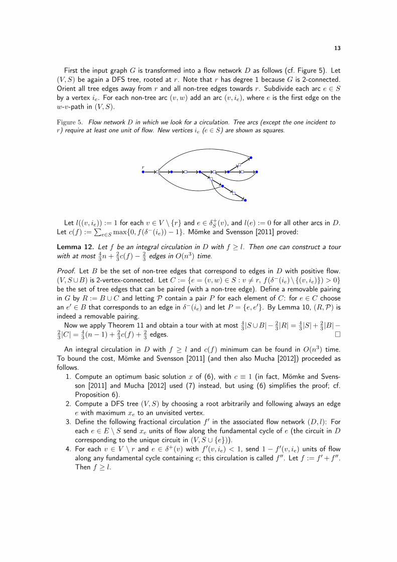
First the input graph G is transformed into a flow network D as follows (cf. Figure 5). Let(V, S) be again a DFS tree, rooted at r. Note that r has degree 1 because G is 2-connected.Orient all tree edges away from r and all non-tree edges towards r. Subdivide each arc e ∈ Sby a vertex ie. For each non-tree arc (v, w) add an arc (v, ie), where e is the first edge on thew-v-path in (V, S).

Figure 5. Flow network D in which we look for a circulation. Tree arcs (except the one incident tor) require at least one unit of flow. New vertices ie (e ∈ S) are shown as squares.

r

Let l((v, ie)) := 1 for each v ∈ V \ r and e ∈ δ+S (v), and l(e) := 0 for all other arcs in D.

Let c(f) :=∑

e∈S max0, f(δ−(ie))− 1. Mömke and Svensson [2011] proved:

Lemma 12. Let f be an integral circulation in D with f ≥ l. Then one can construct a tourwith at most 4

3n+ 23c(f)− 2

3 edges in O(n3) time.

Proof. Let B be the set of non-tree edges that correspond to edges in D with positive flow.(V, S∪B) is 2-vertex-connected. Let C := e = (v, w) ∈ S : v 6= r, f(δ−(ie)\(v, ie)) > 0be the set of tree edges that can be paired (with a non-tree edge). Define a removable pairingin G by R := B ∪ C and letting P contain a pair P for each element of C: for e ∈ C choosean e′ ∈ B that corresponds to an edge in δ−(ie) and let P = e, e′. By Lemma 10, (R,P) isindeed a removable pairing.

Now we apply Theorem 11 and obtain a tour with at most 43 |S ∪B|−

23 |R| =

43 |S|+

23 |B|−

23 |C| =

43(n− 1) + 2

3c(f) + 23 edges.

An integral circulation in D with f ≥ l and c(f) minimum can be found in O(n3) time.To bound the cost, Mömke and Svensson [2011] (and then also Mucha [2012]) proceeded asfollows.

1. Compute an optimum basic solution x of (6), with c ≡ 1 (in fact, Mömke and Svens-son [2011] and Mucha [2012] used (7) instead, but using (6) simplifies the proof; cf.Proposition 6).

2. Compute a DFS tree (V, S) by choosing a root arbitrarily and following always an edgee with maximum xe to an unvisited vertex.

3. Define the following fractional circulation f ′ in the associated flow network (D, l): Foreach e ∈ E \ S send xe units of flow along the fundamental cycle of e (the circuit in Dcorresponding to the unique circuit in (V, S ∪ e)).

4. For each v ∈ V \ r and e ∈ δ+(v) with f ′(v, ie) < 1, send 1 − f ′(v, ie) units of flowalong any fundamental cycle containing e; this circulation is called f ′′. Let f := f ′+ f ′′.Then f ≥ l.

14

Mömke and Svensson [2011] proved c(f) ≤ (4√

2 − 3)x(E) − (6√

2 − 6)n. Mucha [2012]improved the analysis and obtained c(f) ≤ 5

3x(E) − 32n. The heart of his proof consists of

showing that for each v ∈ V \r the contribution of the edges in Bv := e ∈ δ−(v) : xe > 0to c(f) plus the extra flow added for v in step 4 is at most 1

6 |Bv|+56(x(δ(v))− 2); the result

then follows from summation, using the fact that x has at most 2n− 3 nonzero variables (cf.Section 2.9).

We do not know whether Mucha’s bound is tight. Together with Lemma 12 it directly yields a139 -approximation algorithm for the Graphic TSP: we get a tour with at most 4

3n+ 109 x(E)−n

edges.In the case that x in Step 1 is half-integral, we actually get a 4

3 -approximation (as observedby Mömke and Svensson [2011]): we may assume that the support graph is 2-connected(otherwise consider its blocks separately); then f ′′ ≡ 0 and c(f) = 0. This is particularlyinteresting because Schalekamp, Williamson and van Zuylen [2012] conjectured that the worstcase for the integrality ratio occurs when x is an optimum fractional perfect simple 2-matching(and hence w.l.o.g. half-integral).

5 Using ear-decompositions and matroids5.1 Ear-decompositionsAn ear-decomposition of a connected graph G = (V,E) is a sequence P0, P1, . . . , Pk of sub-graphs of G such that P0 consists of a single vertex, E(P1), . . . , E(Pk) is a partition of E,and for i = 1, . . . , k, either Pi is a path with exactly its endpoints in V (P0)∪ · · · ∪ V (Pi−1) orPi is a circuit with exactly one of its vertices (called its endpoint) in V (P0) ∪ · · · ∪ V (Pi−1).

The vertices of an ear that are not endpoints are called its internal vertices. The length ofan ear is the number of its edges; this is always the number of internal vertices plus one. Anear is called trivial if it has length 1, otherwise nontrivial. We call an ear short if it has length2 or 3, otherwise long. An ear is called odd if its length is odd, otherwise even. The numberof ears is always |E| − |V |+ 1. See Figure 6, left-hand side, for an example.

Whitney [1932] observed that a graph is 2-edge-connected if and only if it has an ear-decomposition. Hence computing an ear-decomposition with minimum number of nontrivialears is equivalent to finding the smallest 2-edge-connected spanning subgraph (2ECSS); thisproblem is NP-hard. However, the number of even ears can be minimized in polynomial time.This is a fundamental result of Frank [1993] (also proved in Schrijver’s [2003] book):

Theorem 13. Let G = (V,E) be a 2-edge-connected graph. Let ϕ(G) denote the minimumnumber of even ears in any ear-decomposition of G. Then for any T ⊆ V such that |T | is even,there exists a T -join in G with at most 1

2(|V | + ϕ(G) − 1) edges. Moreover, there exists aT ⊆ V such that |T | is even and the minimum cardinality of a T -join in G is 1

2(|V |+ϕ(G)−1).Such a T and an ear-decomposition with ϕ(G) even ears can be found in O(|V ||E|) time.

Any 2-edge-connected spanning subgraph (2ECSS) of G has at least ϕ(G) ears in any ear-decomposition. Hence any 2ECSS, and thus any tour, has at least n−1+ϕ(G) edges. Cheriyan,Sebő and Szigeti [2001] used Theorem 13 to strengthen this statement. Let

LP(G) := minx(E) : x ≥ 0, x(δ(U)) ≥ 2 (∅ 6= U ⊂ V ). (9)

Note that (9) is the special case of (7) for c(e) = 1 for all e ∈ E, and LP(G) is a lowerbound on the length of an optimum tour.

15

Corollary 14. For any 2-edge-connected graph G we have

Lϕ := n− 1 + ϕ(G) ≤ LP(G).

Proof. By Theorem 13 there exists a set T of vertices such that |T | is even and 12(n−1+ϕ(G))

is the minimum cardinality of a T -join in G. Now observe that (4) is at most half of (7).

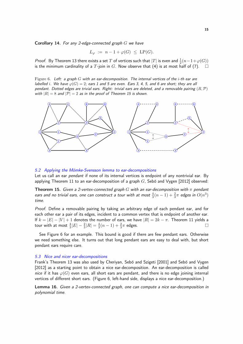
Figure 6. Left: a graph G with an ear-decomposition. The internal vertices of the i-th ear arelabelled i. We have ϕ(G) = 2; ears 1 and 5 are even. Ears 3, 4, 5, and 6 are short; they are allpendant. Dotted edges are trivial ears. Right: trivial ears are deleted, and a removable pairing (R,P)with |R| = 8 and |P| = 2 as in the proof of Theorem 15 is shown.

0

1

1

2 2

22

3 3

4 4

5

6 6

1

0

1

1

2 2

22

3 3

4 4

5

6 6

1

5.2 Applying the Mömke-Svensson lemma to ear-decompositionsLet us call an ear pendant if none of its internal vertices is endpoint of any nontrivial ear. Byapplying Theorem 11 to an ear-decomposition of a graph G, Sebő and Vygen [2012] observed:

Theorem 15. Given a 2-vertex-connected graph G with an ear-decomposition with π pendantears and no trivial ears, one can construct a tour with at most 4

3(n− 1) + 23π edges in O(n3)

time.

Proof. Define a removable pairing by taking an arbitrary edge of each pendant ear, and foreach other ear a pair of its edges, incident to a common vertex that is endpoint of another ear.If k = |E| − |V |+ 1 denotes the number of ears, we have |R| = 2k − π. Theorem 11 yields atour with at most 4

3 |E| −23 |R| =

43(n− 1) + 2

3π edges.

See Figure 6 for an example. This bound is good if there are few pendant ears. Otherwisewe need something else. It turns out that long pendant ears are easy to deal with, but shortpendant ears require care.

5.3 Nice and nicer ear-decompositionsFrank’s Theorem 13 was also used by Cheriyan, Sebő and Szigeti [2001] and Sebő and Vygen[2012] as a starting point to obtain a nice ear-decomposition. An ear-decomposition is callednice if it has ϕ(G) even ears, all short ears are pendant, and there is no edge joining internalvertices of different short ears. (Figure 6, left-hand side, displays a nice ear-decomposition.)

Lemma 16. Given a 2-vertex-connected graph, one can compute a nice ear-decomposition inpolynomial time.

16

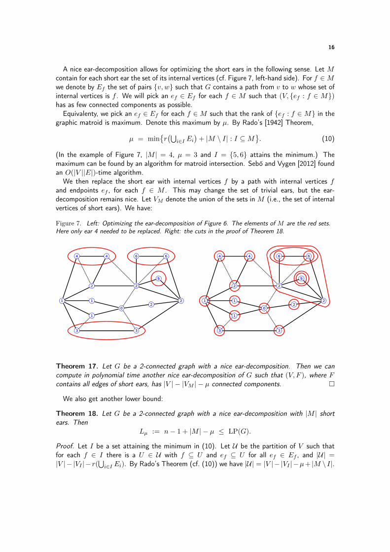
A nice ear-decomposition allows for optimizing the short ears in the following sense. Let Mcontain for each short ear the set of its internal vertices (cf. Figure 7, left-hand side). For f ∈Mwe denote by Ef the set of pairs v, w such that G contains a path from v to w whose set ofinternal vertices is f . We will pick an ef ∈ Ef for each f ∈ M such that (V, ef : f ∈ M)has as few connected components as possible.

Equivalenty, we pick an ef ∈ Ef for each f ∈M such that the rank of ef : f ∈M in thegraphic matroid is maximum. Denote this maximum by µ. By Rado’s [1942] Theorem,

µ = minr(⋃

i∈I Ei)

+ |M \ I| : I ⊆M. (10)

(In the example of Figure 7, |M | = 4, µ = 3 and I = 5, 6 attains the minimum.) Themaximum can be found by an algorithm for matroid intersection. Sebő and Vygen [2012] foundan O(|V ||E|)-time algorithm.

We then replace the short ear with internal vertices f by a path with internal vertices fand endpoints ef , for each f ∈ M . This may change the set of trivial ears, but the ear-decomposition remains nice. Let VM denote the union of the sets in M (i.e., the set of internalvertices of short ears). We have:

Figure 7. Left: Optimizing the ear-decomposition of Figure 6. The elements of M are the red sets.Here only ear 4 needed to be replaced. Right: the cuts in the proof of Theorem 18.

0

1

1

2 2

22

3 3

4 4

5

6 6

1

0

1

1

2 2

22

3 3

4 4

5

6 6

1

Theorem 17. Let G be a 2-connected graph with a nice ear-decomposition. Then we cancompute in polynomial time another nice ear-decomposition of G such that (V, F ), where Fcontains all edges of short ears, has |V | − |VM | − µ connected components.

We also get another lower bound:

Theorem 18. Let G be a 2-connected graph with a nice ear-decomposition with |M | shortears. Then

Lµ := n− 1 + |M | − µ ≤ LP(G).

Proof. Let I be a set attaining the minimum in (10). Let U be the partition of V such thatfor each f ∈ I there is a U ∈ U with f ⊆ U and ef ⊆ U for all ef ∈ Ef , and |U| =|V |− |VI |− r(

⋃i∈I Ei). By Rado’s Theorem (cf. (10)) we have |U| = |V |− |VI |−µ+ |M \ I|.

17

Consider the family of sets U ∪ I.∪ v : v ∈ VI, taking singletons in I twice. Summing

over the inequalities x(δ(U)) ≥ 2 for these sets U (unless U = V ) completes the proof becauseno edge is contained in more than two of these at least n− 1 + |M | − µ cuts.

See Figure 7 (right-hand side) for an illustration. The set F in Theorem 17 consists of theblack edges in Figure 8, left-hand side.

5.4 The 75 -approximation algorithm

Now we can explain the 75 -approximation algorithm for the Graphic TSP by Sebő and Vygen

[2012]. Let ΛG := 23Lµ + 1

3Lϕ. Note that ΛG is a lower bound on the optimum and in fact onLP(G), and ΛG ≥ n− 1 (cf. Corollary 14 and Theorem 18). We first show:

Lemma 19. Let G be a 2-vertex-connected graph with a nice ear-decomposition that has notrivial ears and for which the union of all short ears have |V |−|VM |−µ connected components.Then one can compute a tour in G with at most 7

5Λ edges in O(n3) time.

Proof. If π ≤ Λ10 , apply Theorem 15 and obtain a tour with at most 4

3(n − 1) + 23π ≤

75Λ

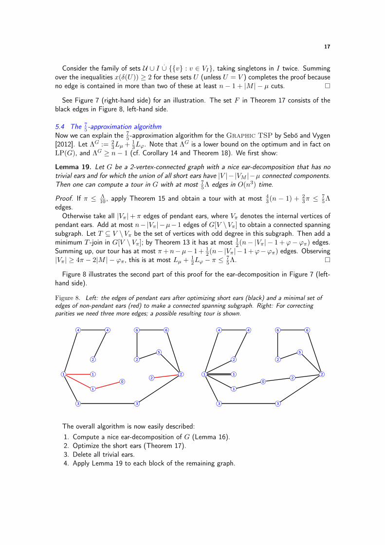
edges.Otherwise take all |Vπ|+ π edges of pendant ears, where Vπ denotes the internal vertices of

pendant ears. Add at most n−|Vπ|−µ−1 edges of G[V \Vπ] to obtain a connected spanningsubgraph. Let T ⊆ V \Vπ be the set of vertices with odd degree in this subgraph. Then add aminimum T -join in G[V \ Vπ]; by Theorem 13 it has at most 1

2(n− |Vπ| − 1 +ϕ−ϕπ) edges.Summing up, our tour has at most π+n−µ− 1 + 1

2(n− |Vπ| − 1 +ϕ−ϕπ) edges. Observing|Vπ| ≥ 4π − 2|M | − ϕπ, this is at most Lµ + 1

2Lϕ − π ≤75Λ.

Figure 8 illustrates the second part of this proof for the ear-decomposition in Figure 7 (left-hand side).

Figure 8. Left: the edges of pendant ears after optimizing short ears (black) and a minimal set ofedges of non-pendant ears (red) to make a connected spanning subgraph. Right: For correctingparities we need three more edges; a possible resulting tour is shown.

0

1

1

2 2

22

3 3

4 4

5

6 6

1

0

1

1

2 2

22

3 3

4 4

5

6 6

1

The overall algorithm is now easily described:1. Compute a nice ear-decomposition of G (Lemma 16).2. Optimize the short ears (Theorem 17).3. Delete all trivial ears.4. Apply Lemma 19 to each block of the remaining graph.

18

It is not difficult to show that the sum of the lower bounds Λ for all blocks equals the lowerbound Λ for G. This implies that we have a 7

5 -approximation algorithm.

6 The path version and connected T -joinsWhat if we do not require the walk to be closed? Then we look for a (Hamiltonian) path inthe metric closure. We assume that the endpoints are given (otherwise we can try all pairs, ortake a tour and delete one edge) and distinct: the path must begin in s and end in t (wheres, t ∈ V and s 6= t). For any of the problems studied in this paper, this variant is called thes-t-path version or simply the path version.

6.1 Asymmetric path versionObviously, any ρ-approximation for the s-t-path version implies a ρ-approximation algorithmfor the Asymmetric TSP itself: just guess any edge (t, s) in an optimum solution (fix sand try all n − 1 possibilities for t). Feige and Singh [2007] showed that the opposite alsoholds approximately: any ρ-approximation for the Asymmetric TSP implies a (2 + ε)ρ-approximation algorithm for the path version.

6.2 Undirected path version and connected T -joinsIn the undirected case, if we ask for a walk from s to t, by Section 1.3 this is equivalent toask for a connected spanning multi-subgraph in which s and t have odd degree and all othervertices have even degree. It is natural to generalize this further to prescribe arbitrary parities:the Connected T -Join Problem asks for a set F such that (V, F ) is a connected graphand F is a T -join. We call such a set F simply a connected T -join, or a T -tour. Again, F maycontain pairs of parallel edges.

For T = ∅ this is the Symmetric TSP, and for T = s, t this is its s-t-path version.Again we may consider the Graphic special case, where all edges of F must be copies ofedges of the input graph.

Christofides’ [1976] algorithm also works for the Connected T -Join Problem: take aminimum spanning tree (V, S) and add a minimum-weight TS-join, where TS is now the set ofvertices whose degree in (V, S) has the wrong parity (so S is a (TS4T )-join).

However, this generalization of Christofides’ algorithm is only a 53 -approximation algorithm

(Hoogeveen [1991], Sebő and Vygen [2012]). To see this, let (V, S) be a minimum spanningtree. Let J be a minimum weight TS-join, and J∗ an optimum solution (a minimum weightconnected T -join). Then S

.∪ J∗ is a TS-join. Since both S and J∗ are connected, each

contains a TS-join; so S.∪ J∗ can be partitioned into three TS-joins. Hence 3c(S

.∪ J) ≤

3c(S) + 3c(J) ≤ 3c(S) + c(S.∪ J∗) = 4c(S) + c(J∗) ≤ 5c(J∗). The bound is tight even for

|T | = 2 (Hoogeveen [1991]), as the graphs (0, . . . , 3k, i, i+ 1 : 0 ≤ i < 3k ∪ 3i, 3i+3 : 0 ≤ i < k) show.

Sebő and Vygen [2012] showed that their techniques (outlined in Section 5 above) also leadto a 3

2 -approximation algorithm for the Graphic Connected T -Join Problem. Previ-ously, there were only algorithms for the special case |T | = 2; here the best was the 1.578-approximation algorithm of An, Kleinberg and Shmoys [2012].

6.3 Best-of-many Christofides’ algorithmAn, Kleinberg and Shmoys [2012] also found a 1.619-approximation algorithm for the path ver-

19

sion (|T | = 2) with general weights. This was the first improvement of Christofides’ algorithmthat is not restricted to the graphic special case. This algorithm was generalized by Cheriyan,Friggstad and Gao [2012]; they obtain an approximation ratio of 1.625 for |T | ≥ 4. Then Sebő[2012] obtained an 8

5 -approximation algorithm for arbitrary T and general weights.All these three papers analyze essentially the same algorithm, which An, Kleinberg and

Shmoys [2012] called best-of-many Christofides: it computes an optimum solution to a naturalLP relaxation (see (11) below) and writes it as convex combination of spanning trees (plus anonnegative vector). For each of these spanning trees, S, we again compute a minimum weightTS-join J , where TS is the set of vertices of S whose degree has the wrong parity, and outputthe best of these T -tours S

.∪ J .

Following Sebő and Vygen [2012] and Sebő [2012], we consider the LP relaxation

min c(x)

subject to x(δ(U)) ≥ 2 (∅ 6= U ⊂ V, |U ∩ T | even)x(δ(W)) ≥ |W|−1 (W partition of V )

xe ≥ 0 (e ∈ E)

(11)

Here δ(W) denotes the set of edges with endpoints in different classes of the partition W.For an optimum solution x (in fact for every feasible solution) we can write x ≥

∑S∈S pSχ

S ,where again S denotes the set of edge sets of spanning trees, χS denotes the incidence vectorof S, and pS ≥ 0 for all S ∈ S and

∑S∈S pS = 1. (An, Kleinberg and Shmoys [2012] and

Cheriyan, Friggstad and Gao [2012] work in the metric closure and use a stronger LP in orderto obtain x =

∑S∈S pSχ

S , but this is not necessary.)By Carathéodory’s theorem we can assume that pS > 0 for less than n2 spanning trees (V, S).

An optimum LP solution x, such spanning trees, and such numbers pS can be computed inpolynomial time, as can be shown with the ellipsoid method. For each S ∈ S with pS > 0,the algorithm computes a minimum weight TS-join J and consider the T -tour S

.∪ J ; we

output the best of these. Its cost is minS∈S: pS>0(c(S) + minc(J) : J is a TS-join) ≤∑S∈S pS(c(S) + minc(J) : J is a TS-join) ≤ c(x) +

∑S∈S pSc(y

S), for any set of vectors(yS)S∈S such that yS is in the TS-join polyhedron (cf. (4)). The difficulty in the analysis liesin finding an appropriate set of vectors (yS)S∈S .

6.4 AnalysisLet Q := Q = δ(U) : ∅ 6= U ⊂ V, x(Q) < 2. An, Kleinberg and Shmoys [2012] proposed tochoose yS := (1− 2β)χS + βx+ rS , where β ≤ 1

2 and rS is a nonnegative vector satisfying

rS(Q) ≥ 4β − 1− βx(Q) (12)

for all S ∈ S and all Q ∈ Q with |Q ∩ S| ≥ 2.Then for each S ∈ S and each TS-cut Q we have yS(Q) ≥ 1. Indeed, if Q /∈ Q, then

yS(Q) ≥ (1 − 2β)|S ∩ Q| + βx(Q) ≥ 1 − 2β + 2β = 1. If Q ∈ Q, then Q is not only aTS-cut but also a T -cut, so |Q ∩ S| is even and hence at least two, and we have yS(Q) =(1− 2β)|Q ∩ S|+ βx(Q) + rS(Q) ≥ 2− 4β + βx(Q) + rS(Q) ≥ 1.

So yS is in the TS-join polyhedron for all S ∈ S. Moreover,∑

S∈S pSc(yS) ≤ (1 −

2β)∑

S∈S pSc(S) + βc(x) +∑

S∈S pSc(rS) ≤ (1− β)c(x) +

∑S∈S pSc(r

S).An, Kleinberg and Shmoys [2012] chose β = 1/

√5 and found a vector r such that rS = r for

all S ∈ S satisfies (12) and c(r) ≤ (7√

5−15)/10, yielding the approximation ratio (1+√

5)/2(the golden ratio).

20

Sebő [2012] improved this by letting vQ :=∑

S∈S:|Q∩S|=1 pSχQ∩S for Q ∈ Q, and

rS :=∑

Q∈Q:|Q∩S|≥2

max

0,

4β − 1− βx(Q)

2− x(Q)

vQ.

Note that vQ(Q) =∑

S∈S:|Q∩S|=1 pS ≥ 2−∑

S∈S pS |Q∩S| ≥ 2−x(Q). To show (12), simply

observe that for S ∈ S and Q ∈ Q with |Q ∩ S| = 2 we have rS(Q) ≥ 4β−1−βx(Q)2−x(Q) vQ(Q).

We now bound the cost. Note that∑

S∈S:|Q∩S|≥2 pS ≤ x(Q) − 1 for Q ∈ Q. Using

this, we obtain the bound∑

S∈S pSc(rS) ≤

∑Q∈Q(x(Q)− 1) max

0, 4β−1−βx(Q)

2−x(Q)

c(vQ) ≤∑

Q∈Q19c(v

Q) = 19

∑S∈S pS

∑Q∈Q:|Q∩S|=1 c(Q∩S) ≤ 1

9

∑S∈S pSc(S\JS), where JS denotes

the unique subset of S that is a TS-join.Let β = 4

9 . If∑

S∈S pSc(S \ JS) ≤ 25c(x), we have

∑S∈S pSc(y

S) ≤ (1 − 49 + 2

45)c(x) =35c(x). Otherwise

∑S∈S pSc(JS) ≤ 3

5c(x), and noting that χJS is in the TS-join polyhedron,we get the same bound. This gives Sebő’s [2012] 8

5 -approximation algorithm.

7 Further resultsWe briefly mention some other related results. However, it is impossible to mention all importantresults here.

7.1 InapproximabilityLampis [2012] proved that no 185

184 -approximation algorithm exists for the Symmetric TSPunless P = NP. Papadimitriou and Vempala [2006] proved that no 118

117 -approximation algorithmexists for the Asymmetric TSP unless P = NP.

7.2 Integrality RatiosWe have seen in Section 2.2 that the integrality ratio of (2) is at least 4

3 even for graphicmetrics. The integrality ratio of (2) is conjectured to be exactly 4

3 even for general metrics,but this so-called TSP-4

3 -conjecture is open; we only know Wolsey’s [1980] upper bound 32 in

general (cf. Section 2.5) and the upper bound 75 for graphic metrics by Sebő and Vygen [2012]

(cf. Section 5).The TSP-4

3 -conjecture is supported by computational verification for n ≤ 12 (Boyd andElliott-Magwood [2007]) and by theoretical work of Goemans [1995], who proved that for anyinstance with ratio greater than 4

3 even the LP that arises from (7) by adding many classesof inequalities that are valid for the graphical traveling salesman polyhedron does not have anintegral optimum solution.

Schalekamp, Williamson and van Zuylen [2012] showed that the worst ratio of an optimumperfect 2-matching over (2) is 10

9 , as conjectured by Boyd and Carr [2011].For (6) and (7), the integrality ratio is between 6

5 and 32 (Alexander, Boyd and Elliott-

Magwood [2006]). Carr and Ravi [1998] conjectured it to be 43 . The ratio restricted to unit

weights is between 98 and 4

3 (Sebő and Vygen [2012]).The integrality ratio of the asymmetric subtour LP is at least 2 (shown by Charikar, Goemans

and Karloff [2006], disproving a conjecture of Carr and Vempala [2004]) and at most 2 +8 lnn/ ln lnn (Asadpour et al. [2010]). The same holds for the path version (Friggstad, Guptaand Singh [2012]).

21

7.3 Further special casesAn even more special case than the Graphic TSP is the 1-2-TSP, in which c(v, w) ∈ 1, 2for all v, w ∈ V . To see that this is essentially a special case of the Graphic TSP (upto an additive constant of 1), add a vertex x and consider the graph (V ∪ x, v, x : v ∈V ∪v, w : v, w ∈ V, u 6= v, c(v, w) = 1) The 1-2-TSP has an 8

7 -approximation algorithm(Berman and Karpinski [2006]) but no 744

743 -approximation algorithm (Engebretsen and Karpinksi[2006]). The integrality ratio of (2) for the 1-2-TSP is between 10

9 and 1915 (Qian et al. [2012]).

In the special case of the Graphic TSP where the instance is a k-regular graph (withk large), Vishnoi [2012] showed how to find a tour of length at most (1 +

√64/ ln k)n in

polynomial time.

7.4 Geometric instances and planar graphsArora [1998] found an approximation scheme for geometric instances. Here, each city is associ-ated with a point in Rd, and the distances are `p-distances. This case is also NP-hard, for anyfixed d ≥ 2 and any p. The most prominent case d = p = 2 is called the Euclidean TSP (seealso Mitchell [1999]). Rao and Smith [1998] improved the running time: for every fixed ε > 0they have a (1 + ε)-approximation algorithm that runs in O(n log n) time. However, the con-stants involved are still quite large for reasonable values of ε, and thus the practical value seemsto be limited. Bartal, Gottlieb and Krauthgamer [2012] found a randomized approximationscheme for metric spaces with bounded doubling dimension.

For planar graphs with nonnegative edge weights, Klein [2008] found an approximationscheme that has linear running time for every fixed ε > 0. An approximation scheme existseven for bounded genus graphs (Demaine, Hajiaghayi and Mohar [2010]).

Interestingly, it is not known whether the decision version of the Euclidean TSP belongsto NP.

7.5 Polyhedral DescriptionsMany classes of facets of the TSP polytope have been discovered, but a complete descriptionis out of reach. Recently, Fiorini et al. [2012] proved that every polyhedron that projects tothe TSP polytope (i.e., any extended formulation) has 2Ω(n1/4) facets. It may not be surprisingthat the TSP has no compact extended formulation, but this was not known before, and thisresult is unconditional (i.e., it does not assume P 6= NP). The proof reveals an interestingconnection to communication complexity.

7.6 The 2ECSS problemThe integral solutions to (6) are the 2-edge-connected spanning subgraphs (2ECSS). Monma,Munson and Pulleyblank [1990] showed that the smallest 2ECSS can be smaller than theshortest tour by up to a factor 4

3 ; this also follows directly from applying Theorem 11 to eachblock of a smallest 2ECSS. The bound is tight as Figure 2 shows.

Sebő and Vygen [2012] observed that the techniques of Section 5 directly imply a 43 -

approximation algorithm for the (unweighted) 2ECSS problem. Indeed, if π ≥ 16LP(G), the

second case of the proof of Lemma 19 yields a tour (and hence a 2ECSS) of length 43LP(G).

Otherwise one can simply take all k nontrivial ears: we get n− 1 +k edges, and this is at most54Lϕ + π

2 since n− 1 ≥ 4k − 2π − ϕ(G).Better approximation ratios have been claimed, but no complete proof has been published.

22

Fernandes [1998] proved that the problem is MAXSNP-hard. For the weighted case, Khullerand Vishkin [1994] found a 2-approximation algorithm, which is still the best known.

Sebő and Vygen [2012] also showed the following: if there is a ρ-approximation algorithmfor the unweighted 2ECSS problem, then there is a 2

3(ρ + 1)-approximation algorithm for theGraphic TSP.

8 Open problemsWe conclude this survey by listing some open research problems that we consider important.Almost all of these problems have been formulated earlier, and indeed most of them are verynatural. None of them seems to be easy. However, given the remarkable progress that has beenmade during the last few years, one may hope that we will see some solutions soon.

1. Improve Christofides’ algorithm: find a ρ-approximation algorithm for the SymmetricTSP for some ρ < 3

2 .

2. Find a constant-factor approximation algorithm for the Asymmetric TSP, or at leastthe special case in which a strongly connected digraph (V,E) is given and c(v, w) = 1 if(v, w) ∈ E and c(v, w) =∞ otherwise (one might call this the Digraphic TSP).

3. Determine the integrality ratio of the subtour relaxation (2) of the Symmetric TSP.

4. Prove a better bound on the integrality ratio for another (polynomial-time solvable) LPrelaxation of the Symmetric TSP.

5. Solve the LPs (2), (6), (7), and (8) by combinatorial algorithms.

6. Answer the question whether the integrality ratio of the directed subtour relaxation (8)is bounded by a constant.

7. How good is the best-of-many Christofides’ algorithm (cf. Section 6.3) really; i.e., whatis the worst case? The answer can of course be different for T = ∅ (the SymmetricTSP) and for general T .

8. Improve the lower bounds on the approximability substantially.

9. Find a 43 -approximation algorithm for the Graphic TSP.

10. Find a 32 -approximation algorithm for the Connected T -Join Problem with arbitrary

nonnegative weights, at least in the special case |T | = 2.

11. Improve on the 2-approximation algorithm for the weighted 2ECSS problem. Notethat Wolsey’s analysis (Section 2.5) shows that Christofides’ algorithm is also a 3

2 -approximation algorithm for the variant of the 2ECSS problem where doubling edgesis allowed. However, in contrast to the unweighted special case, allowing to double edgesreally changes the problem.

AcknowledgementThanks to Corinna Gottschalk, Swati Gupta, Satoru Iwata, Volker Kaibel, Marcin Mucha, R.Ravi, András Sebő, David Shmoys, and Ola Svensson for careful reading and useful remarks.

Bibliography

Alexander, A., Boyd, S., and Elliott-Magwood, P. [2006]: On the integrality gap of the 2-edge connectedsubgraph problem. Technical Report TR-2006-04, SITE, University of Ottawa 2006

An, H.-C., Kleinberg, R., and Shmoys, D.B. [2012]: Improving Christofides’ algorithm for the s-t pathTSP. Proceedings of the 44th Annual ACM Symposium on Theory of Computing (STOC 2012),875–886

Applegate, D.L., Bixby, R., Chvátal, V., and Cook, W.J. [2006]: The Traveling Salesman Problem: AComputational Study. Princeton University Press 2006

Arora, S. [1998]: Polynomial time approximation schemes for Euclidean traveling salesman and othergeometric problems. Journal of the ACM 45 (1998), 753–782

Asadpour, A., Goemans, M.X., Mądry, A., Oveis Gharan, S., and Saberi, A. [2010]: AnO(log n/ log log n)-approximation algorithm for the asymmetric traveling salesman problem. Pro-ceedings of the 21st Annual ACM-SIAM Symposium on Discrete Algorithms (SODA 2010), 379–389

Bartal, Y., Gottlieb, L.-A., and Krauthgamer, R. [2012]: The traveling salesman problem: low-dimensionality implies a polynomial time approximation scheme. Proceedings of the 44th AnnualACM Symposium on Theory of Computing (STOC 2012), 663–672

Berman, P., and Karpinski, M. [2006]: 8/7-approximation algorithm for (1,2)-TSP. Proceedings of the17th Annual ACM-SIAM Symposium on Discrete Algorithms (SODA 2006), 641–648

Bläser, M. [2003]: A new approximation algorithm for the asymmetric TSP with triangle inequality.Proceedings of the Fourteenth Annual ACM-SIAM Symposium on Discrete Algorithms (SODA 2003),638–645

Boyd, S., and Carr, R. [2011]: Finding low cost TSP and 2-matching solutions using certain half-integersubtour vertices. Discrete Optimization 8 (2011), 525–539

Boyd, S., and Elliott-Magwood, P. [2007]: Structure of the extreme points of the subtour eliminationpolytope of the STSP. Technical Report TR-2007-09, SITE, University of Ottawa, Ottawa, 2007

Boyd, S., Sitters, R., van der Ster, S., and Stougie, L. [2011]: TSP on cubic and subcubic graphs. In:Integer Programming and Combinatorial Optimization; Proceedings of the 15th International IPCOConference; LNCS 6655 (O. Günlük, G.J. Woeginger, eds.), Springer, Berlin 2011, pp. 65–77

Carr, R., and Ravi, R. [1998]: A new bound for the 2-edge connected subgraph problem. In: IntegerProgramming and Combinatorial Optimization; Proceedings of the 6th International IPCO Confer-ence; LNCS 1412 (R.E. Bixby, E.A. Boyd, R.Z. Ríos-Mercado, eds.), Springer, Berlin 1998; pp.112-125

Carr, R., and Vempala, S. [2004]: On the Held-Karp relxation for the asymmetric and symmetrictraveling salesman problems. Mathematical Programming A 100 (2004), 569–587

Charikar, M., Goemans, M.X., and Karloff, H. [2006]: On the integrality ratio for the asymmetrictraveling salesman problem. Mathematics of Operations Research 31 (2006), 245–252

23

24

Chekuri, C., Vondrák, J., and Zenklusen, R. [2010]: Dependent randomized rounding via exchange prop-erties of combinatorial structures. Proceedings of the 51st Annual IEEE Symposium on Foundationsof Computer Science (FOCS 2010), 575–584

Cheriyan, J., Friggstad, Z., and Gao, Z. [2012]: Approximating minimum-cost connected T -joins.Approximation, Randomization, and Combinatorial Optimization; Proceedings of the 16th APPROXWorkshop; LNCS 7408 (A. Gupta, K. Jansen, J. Rolim, R. Servedio, eds.), Springer, Berlin 2012,pp. 110–121

Cheriyan, J., Sebő, A., and Szigeti, Z. [2001]: Improving on the 1.5-approximation of a smallest 2-edgeconnected spanning subgraph. SIAM Journal on Discrete Mathematics 14 (2001), 170–180

Christofides, N. [1976]: Worst-case analysis of a new heuristic for the traveling salesman problem.Technical Report 388, Graduate School of Industrial Administration, Carnegie-Mellon University,Pittsburgh 1976

Cook, W.J. [2012]: In Pursuit of the Traveling Salesman: Mathematics at the Limits of Computation.Princeton University Press 2012

Cornuéjols, G., Fonlupt, J., and Naddef, D. [1985]: The traveling salesman problem on a graph andsome related integer polyhedra. Mathematical Programming 33 (1985), 1–27

Correa, J.R., Larré, O., and Soto, J.A. [2012]: TSP tours in cubic graphs: beyond 4/3. In: Algorithms– ESA 2012; LNCS 7501 (L. Epstein, P. Ferragina, eds.), Springer, Berlin 2012, pp. 790–801

Dantzig, G.B., Fulkerson, D.R., and Johnson, S.M. [1954]: Solution of a large scale traveling salesmanproblem. Operations Research 2 (1954), 393–410

Demaine, E.D., Hajiaghayi, M., and Mohar, B. [2010]: Approximation algorithms via contractiondecomposition. Combinatorica 30 (2010), 533–552

Edmonds, J. [1965]: The Chinese postman’s problem. Bulletin of the Operations Research Society ofAmerica 13 (1965), B-73

Edmonds, J. [1970]: Submodular functions, matroids and certain polyhedra. In: Combinatorial Struc-tures and Their Applications; Proceedings of the Calgary International Conference on CombinatorialStructures and Their Applications 1969 (R. Guy, H. Hanani, N. Sauer, J. Schönheim, eds.), Gordonand Breach, New York 1970, pp. 69–87

Edmonds, J., and Johnson, E.L. [1973]: Matching, Euler tours and the Chinese postman. MathematicalProgramming 5 (1973), 88–124

Engebretsen, L., and Karpinski, M. [2006]: TSP with bounded metrics. Journal of Computer andSystem Sciences 72 (2006), 509–546

Euler, L. [1736]: Solutio problematis ad geometriam situs pertinentis. Commentarii AcademiaePetropolitanae 8 (1736), 128–140

Feige, U., and Singh, M. [2007]: Improved approximation algorithms for traveling salesperson tours andpaths in directed graphs. Proceedings of the 10th International Workshop on Approximation Algo-rithms for Combinatorial Optimization Problems; LNCS 4627 (M. Charikar, K. Jansen, O. Reingold,J.D.P. Rolim, eds.), Springer, Berlin 2007, pp. 104–118

Fernandes, C.G. [1998]: A better approximation ratio for the minimum size k-edge-connected spanningsubgraph problem. Journal of Algorithms 28 (1998), 105–124

Fiorini, S., Massar, S., Pokutta, S., Tiwary, H.R., and de Wolf, R. [2012]: Linear vs. semidefiniteextended formulations: exponential separation and strong lower bounds. Proceedings of the 44thAnnual ACM Symposium on Theory of Computing (STOC 2012), 95–106

25

Frank, A. [1993]: Conservative weightings and ear-decompositions of graphs. Combinatorica 13 (1993),65–81

Frieze, A.M., Galbiati, G., and Maffioli, F. [1982]: On the worst-case performance of some algorithmsfor the asymmetric traveling salesman problem. Networks 12 (1982), 23–39

Friggstad, Z., Gupta, A., and Singh. M. [2012]: An improved integrality gap for asymmetric TSP paths.Accepted for IPCO 2013

Gamarnik D., Lewenstein M., and Sviridenko M. [2005]: An improved upper bound for the TSP incubic 3-edge-connected graphs. Operations Research Letters, 33 (2005), 467–474

Garey, M.R., Johnson, D.S., and Tarjan, R.E. [1976]: The planar Hamiltonian circuit problem isNP-complete. SIAM Journal on Computing 5 (1976), 704–714

Goemans, M.X. [1995]: Worst-case comparison of valid inequalities for the TSP. Mathematical Pro-gramming, 69 (1995), 335–349

Goemans, M.X. [2006]: Minimum bounded-degree spanning trees. Proceedings of the 47th AnnualIEEE Symposium on Foundations of Computer Science (FOCS 2006), 273–282

Goemans, M.X., and Bertsimas, D.J. [1993]: Survivable networks, linear programming relaxations andthe parsimonious property. Mathematical Programming 60 (1993), 145–166

Held, M., and Karp, R.M. [1970]: The traveling-salesman problem and minimum spanning trees.Operations Research 18 (1970), 1138–1162

Hierholzer, C. [1873]: Über die Möglichkeit, einen Linienzug ohne Wiederholung und ohne Unter-brechung zu umfahren. Mathematische Annalen 6 (1873), 30–32

Hoffman, A.J. [1960]: Some recent applications of the theory of linear inequalities to extremal combi-natorial analysis. In: Combinatorial Analysis (R.E. Bellman, M. Hall, eds.), AMS, Providence 1960,pp. 113–128

Hoogeveen, J.A. [1991]: Analysis of Christofides’ heuristic: some paths are more difficult than cycles.Operations Research Letters 10 (1991), 291–295

Kaplan, H., Lewenstein, M., Shafrir, N., and Sviridenko, M. [2005]: Approximation algorithms forasymmetric TSP by decomposing directed regular multigraphs. Journal of the ACM 52 (2005),602–626

Karger, D.R., and Stein, C. [1996]: A new approach to the minimum cut problem. Journal of the ACM43 (1996), 601–640

Karp, R.M. [1972]: Reducibility among combinatorial problems. In: Complexity of Computer Compu-tations (R.E. Miller, J.W. Thatcher, eds.), Plenum Press, New York 1972, pp. 85–103

Khuller, S., and Vishkin, U. [1994]: Biconnectivity approximations and graph carvings. Journal of theACM 41 (1994), 214–235

Klein, P.N. [2008]: A linear-time approximation scheme for TSP in undirected planar graphs withedge-weights. SIAM Journal on Computing 37 (2008), 1926–1952

Korte, B., and Vygen, J. [2012]: Combinatorial Optimization: Theory and Algorithms. Springer, Berlin,Fifth Edition 2012

Lampis, M. [2012]: Improved inapproximability for TSP. Approximation, Randomization, and Combina-torial Optimization; Proceedings of the 16th APPROX Workshop; LNCS 7408 (A. Gupta, K. Jansen,J. Rolim, R. Servedio, eds.), Springer, Berlin 2012, pp. 243–253

Lovász, L. [1976]: On some connectivity properties of Eulerian graphs. Acta Mathematica AcademiaeScientiarum Hungaricae 28 (1976), 129–138

26

Mitchell, J. [1999]: Guillotine subdivisions approximate polygonal subdivisions: a simple polynomial-time approximation scheme for geometric TSP, k-MST, and related problems. SIAM Journal onComputing 28 (1999), 1298–1309

Mömke, T., and Svensson, O. [2011]: Approximating graphic TSP by matchings. Proceedings of the52nd Annual Symposium on Foundations of Computer Science (FOCS 2011), 560–569

Monma, C.L., Munson, B.S., and Pulleyblank, W.R. [1990]: Minimum-weight two-connected spanningnetworks. Mathematical Programming 46 (1990), 153–171

Mucha, M. [2012]: 139 -approximation for graphic TSP. Proceedings of the 29th International Symposium

on Theoretical Aspects of Computer Science (2012), 30–41

Oveis Gharan, S., Saberi, A., and Singh, M. [2011]: A randomized rounding approach to the travelingsalesman problem. Proceedings of the 52nd Annual IEEE Symposium on Foundations of ComputerScience (FOCS 2011), 550–559

Papadimitriou, C.H., and Vempala, S. [2006]: On the approximability of the traveling salesman problem.Combinatorica 26 (2006), 101–120

Papadimitriou, C.H., and Yannakakis, M. [1993]: The traveling salesman problem with distances oneand two. Mathematics of Operations Research 18 (1993), 1–12

Qian, J., Schalekamp, F., Williamson, D.P., and van Zuylen, A. [2012]: On the integrality gap of thesubtour LP for the 1,2-TSP. In: LATIN 2012; Theoretical Informatics; LNCS 7256 (D. Fernández-Baca, ed.), Springer, Berlin 2012, pp. 606–617

Rado, R. [1942]: A theorem on independence relations. Quarterly Journal of Mathematics 13 (1942),83–89

Rao, S.B., and Smith, W.D. [1998]: Approximating geometric graphs via “spanners” and “banyans”.Proceedings of the 30th Annual ACM Symposium on Theory of Computing (STOC 1998), 540–550

Sahni, S., and Gonzalez, T. [1976]: P-complete approximation problems. Journal of the ACM 23(1976), 555–565

Schalekamp, F., Williamson, D.P., and van Zuylen, A. [2012]: A proof of the Boyd-Carr conjecture.Proceedings of the 23rd Annual ACM-SIAM Symposium on Discrete Algorithms (SODA 2012), pp.1477–1486

Schrijver, A. [2003]: Combinatorial Optimization: Polyhedra and Efficiency. Springer, Berlin 2003

Sebő, A. [2012]: Eight fifth approximation for TSP paths. arXiv:1209.3523; accepted for IPCO 2013

Sebő, A., and Vygen, J. [2012]: Shorter tours by nicer ears: 7/5-approximation for graphic TSP, 3/2for the path version, and 4/3 for two-edge-connected subgraphs. arXiv:1201.1870

Vishnoi, N.K. [2012]: A permanent approach to the traveling salesman problem, Proceedings of the53rd Annual IEEE Symposium on Foundations of Computer Science (FOCS 2012), 76–80

Whitney, H. [1932]: Non-separable and planar graphs. Transactions of the American MathematicalSociety 34 (1932), 339–362

Wolsey, L.A. [1980]: Heuristic analysis, linear programming and branch and bound. MathematicalProgramming Study 13 (1980), 121–134