JHEP09(2016)038

Published for SISSA by Springer

Received: July 21, 2016

Accepted: August 31, 2016

Published: September 8, 2016

Modular Hamiltonians for deformed half-spaces and

the averaged null energy condition

Thomas Faulkner, Robert G. Leigh, Onkar Parrikar and Huajia Wang

Department of Physics, University of Illinois,

1110 W. Green St., Urbana IL 61801-3080, U.S.A.

E-mail: tomf@illinois.edu, rgleigh@illinois.edu,

parrika2@illinois.edu, rockwhj@illinois.edu

Abstract: We study modular Hamiltonians corresponding to the vacuum state for de-

formed half-spaces in relativistic quantum field theories on R1,d−1. We show that in addi-

tion to the usual boost generator, there is a contribution to the modular Hamiltonian at

first order in the shape deformation, proportional to the integral of the null components

of the stress tensor along the Rindler horizon. We use this fact along with monotonicity

of relative entropy to prove the averaged null energy condition in Minkowski space-time.

This subsequently gives a new proof of the Hofman-Maldacena bounds on the parameters

appearing in CFT three-point functions. Our main technical advance involves adapting

newly developed perturbative methods for calculating entanglement entropy to the prob-

lem at hand. These methods were recently used to prove certain results on the shape

dependence of entanglement in CFTs and here we generalize these results to excited states

and real time dynamics. We also discuss the AdS/CFT counterpart of this result, mak-

ing connection with the recently proposed gravitational dual for modular Hamiltonians in

holographic theories.

Keywords: AdS-CFT Correspondence, Field Theories in Higher Dimensions

ArXiv ePrint: 1605.08072

Open Access, c© The Authors.

Article funded by SCOAP3.doi:10.1007/JHEP09(2016)038

JHEP09(2016)038

Contents

1 Introduction 1

1.1 Setup & summary of results 3

2 Modular Hamiltonian for deformed half-space 7

2.1 Reduced density matrix 7

2.2 Modular Hamiltonian 9

3 Averaged null energy condition 15

3.1 Positivity of KA0 − KA 15

3.2 Computing 〈KA0〉ψ − 〈KA〉ψ 16

4 Modular Hamiltonians in AdS/CFT 17

5 Discussion 21

5.1 Sharpening the argument 22

5.2 Generalizations 23

A Cutoff at the entangling surface 25

1 Introduction

The entanglement structure of states is of great importance in quantum field theory. The

most common tool used for studying entanglement structure is the entanglement entropy,

namely the Von Neumann entropy of a subregion, and has already provided many important

insights. A more fine-grained probe is the modular Hamiltonian, defined as

KΨA = −ln ρΨ

A (1.1)

where ρΨA is the reduced density matrix of the state Ψ over the subregion A. The modular

Hamiltonian is, in general, a complicated, non-local operator and not of much practical use.

However, the situation greatly simplifies for the vacuum state in the case of certain special

symmetric subregions. For instance, the modular Hamiltonian for a half-space in relativistic

quantum field theories takes a very simple form; it is the restriction to the half space of the

generator of boosts which preserve the entangling surface [1], and consequently generates

a local and geometric modular flow. A similar construction is also possible for spherical

subregions in conformal field theories [2], for null slabs in the case where the vacuum state

is defined with respect to the generator of null translations on a null hypersurface [3, 4]

etc. Recently, it has been argued that the modular Hamiltonian for states with classical

gravitational duals also takes a simple form [5, 6]. On the other hand, it is quite non-trivial

– 1 –

JHEP09(2016)038

to study the entanglement entropy and modular Hamiltonian for more general (asymmetric)

subregions, especially outside the purview of free-field theories or AdS/CFT. Some progress

was made in [7] (following previous work in [8–12]), where perturbative techniques were

used to study the shape-dependence of entanglement entropy in conformal field theories. In

the present paper, we adapt these techniques to study modular Hamiltonians for deformed

half-spaces in relativistic (not necessarily conformal) quantum field theories.

The study of shape dependence of entanglement is an important task for several rea-

sons. The entanglement structure of quantum systems is highly constrained by powerful

inequalities, such as strong subadditivity of entanglement entropy, positivity and mono-

tonicity of relative entropy, etc. In many situations, these entanglement inequalities further

imply fundamental constraints on the properties of quantum field theories. For instance,

the strong subadditivity property was used in [13, 14] to prove an entropic version of the

c-theorem for renormalization group flows in two and three dimensions. Similarly, the

properties of relative entropy have been used to prove several interesting results such as

the Bekenstein bound [15], the generalized second law for causal horizons [16] and the

covariant entropy bound in the context of semi-classical gravity [3, 4]. Entanglement in-

equalities have also been shown to constrain the bulk geometry in states with classical

gravity duals [17–20]. The entanglement inequality which will be relevant for our purpose

is that the full modular Hamiltonian for the vacuum state

KA = KA −KAc (1.2)

(i.e., the difference between the modular Hamiltonian of the subregion A and that of the

complementary subregion Ac) satisfies a “monotonicity” property under inclusion [21]. This

means that if we shrink the subregion A, then the corresponding change in the full modular

Hamiltonian δKA is a negative semi-definite operator. This property in fact follows from

the monotonicity of relative entropy, as was shown in [22]. In the present work, we will show

that this monotonicity property of the full modular Hamiltonian along with perturbative

results on the shape dependence of the modular Hamiltonian allow us to prove another

fundamental constraint, namely the averaged null energy condition (ANEC)

∫ ∞

−∞dx+

⟨T++(x+, x− = 0, ~xi)

⟩ψ≥ 0 (1.3)

for excited state in relativistic quantum field theories on Minkowski space-time.

From a classical general relativity point of view, averaged energy conditions (which are

weaker than the point-wise null, weak, strong, dominant-energy conditions) were shown

to be sufficient for proving a number of interesting results such as standard focussing

theorems [23, 24], topological censorship [25], etc. This provides a clear motivation for

trying to prove or disprove averaged energy conditions for quantum fields in general space-

times, given that most point-wise conditions are known to be violated by quantum effects

(see for instance, [26]).1 In Minkowski space-time, the ANEC has been proven to hold

1However, there are alternative proposals for point-wise quantum energy conditions. See for

example [27–29].

– 2 –

JHEP09(2016)038

for many special cases such as free scalar and Maxwell fields in general dimension [30–32],

arbitrary quantum field theories in d = 2 with a mass gap and some assumptions on the

stress tensor [33], CFTs with classical gravitational duals in general dimension [34], etc.

Wall has also argued that the ANEC holds true for free or superrenormalizable field theories

in general dimension [16]. In summary, there is substantial evidence so far to suggest that

the ANEC is satisfied by generic quantum field theories on Minkowski space-time, but a

general proof has been missing hitherto (although see [35] for an argument involving certain

assumptions on the OPE of non-local operators) — in this paper, we will partially fill this

gap. On the other hand, the ANEC is known to be violated in general curved space-times,

but an alternative proposal called the self-consistent achronal ANEC exists in this case —

see [36–38] and references there-in for further discussion. While this is out of the scope

of the present paper, our results can nevertheless be extended to prove the ANEC along

static bifurcate Killing horizons even in curved space-times.

There is another motivation for trying to prove the ANEC in Minkowski space-time.

In [39], Hofman and Maldacena (HM) showed that in a conformal field theory the validity of

the ANEC in a certain class of states created by operator insertions implies bounds on the

coefficients appearing in the three-point correlation functions of that CFT. For instance,

in d = 4 they used this to derive a bound on the ratio of central charges

1

3≤ a

c≤ 31

18(1.4)

where a and c are the coefficients of the Euler density term and the Weyl tensor squared

term in the conformal anomaly; tighter bounds can be obtained by imposing supersymme-

try. While the assumption of the ANEC was considered reasonable, in the original paper

no proof was given. Since then, there have been several attempts at a proof of the HM

bounds with varying levels of success [35, 40, 41].

In particular, using analytic bootstrap methods the HM bounds were proven for a class

of three-point functions in [42], building on the work of [43, 44]. These methods take as an

input crossing symmetry and reflection positivity and apply these principles to various four

point functions in a light-cone limit to delicately extract the HM bounds. In particular in

this guise the HM bounds were related to causality properties of correlation functions in

a shockwave background [44].2 In contrast, we will show that the general HM constraints

on CFT three-point functions can be extracted directly from the three-point function itself

- when the three-point function is interpreted as calculating some modular energy of the

CFT in an excited state.

Overall it is satisfying to see the ANEC, and consequently the Hofman-Maldacena

bounds, arise as a natural consequence of the fundamental constraints satisfied by the

entanglement structure of the vacuum.

1.1 Setup & summary of results

We now outline the calculation we are interested in, and present a brief summary of our

results. Consider the density matrix |Ψ〉〈Ψ| corresponding to a pure state defined on the

2In theories with gravity duals, the HM bounds have also been shown to be related to bulk causality

constraints [34, 35, 45, 46].

– 3 –

JHEP09(2016)038

Cauchy surface Σ. Let us partition Σ into two subregions A and its complement Ac. For

local quantum field theories, we expect the Hilbert space hΣ to factorize into the tensor

product hΣ = hA ⊗ hAc . If this is the case, we can trace over hAc to obtain the reduced

density matrix

ρΨA = TrAc(|Ψ〉〈Ψ|) (1.5)

which contains all the relevant information pertaining to the subregion A. The entangle-

ment entropy between A and Ac is defined as the von Neumann entropy of ρΨA

SEE[Ψ, A] = −TrA(ρΨA ln ρΨ

A

). (1.6)

In this context, the boundary ∂A of A is referred to as the entangling surface. The modular

Hamiltonian (also known as the entanglement Hamiltonian) KΨA is defined as

KΨA = −ln ρΨ

A (1.7)

Similarly, we can also define the modular Hamiltonian corresponding to the region Ac,

which we denote KΨAc . We can combine KΨ

A and KΨAc into another useful operator:

KΨA = KΨ

A ⊗ 1Ac − 1A ⊗KΨAc (1.8)

which we will refer to as the full modular Hamiltonian.

In this paper, we will primarily study the operators KA, KAc and KA for the vacuum

state of a relativistic quantum field theory (as such we drop the label Ψ from now on), with

the region A being a slightly deformed half-space. To specify the geometry in more detail,

let us pick global coordinates xµ = (x0, x1, · · · , xd−1) = (x0,x) on R1,d−1, where x0 is the

time coordinate, and x denotes spatial coordinates. Pick the Cauchy surface Σ given by

x0 = 0, and consider the half space A0 given by

A0 ={xµ ∈ R1,d−1|x0 = 0, x1 > 0

}. (1.9)

The vacuum modular Hamiltonian for the half space takes a particularly simple form [1]

KA0 = 2π

∫

A0

dd−1xx1 T00(0,x) + constant (1.10)

i.e., it is the generator of boosts which preserve the entangling surface restricted to the

region A0, a result known as the Bisognano-Wichmann theorem [1]. Correspondingly, the

full modular Hamiltonian is given by the full boost generator

KA0 = 2π

∫

Σdd−1xx1 T00(0,x) (1.11)

Note that KA0 is a conserved charge, and as such annihilates the vacuum KA0 |0〉 = 0.

(This later property is true for more general regions as well.)

One can consider a small deformation of the region A0 to

A ={xµ ∈ R1,d−1

∣∣∣ x0 = 0, x1 > ζ(~x)}

(1.12)

– 4 –

JHEP09(2016)038

H+

H�

Hc�

Hc+

A0

A

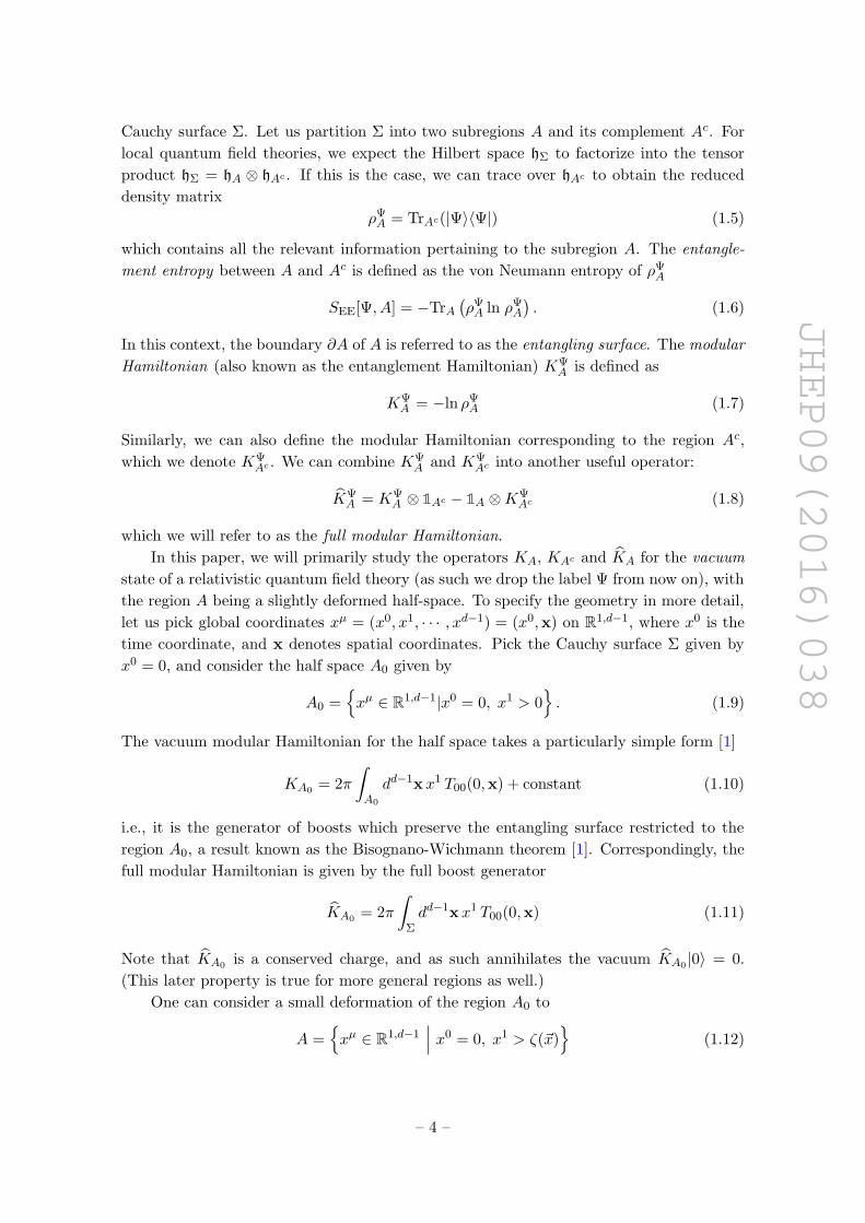
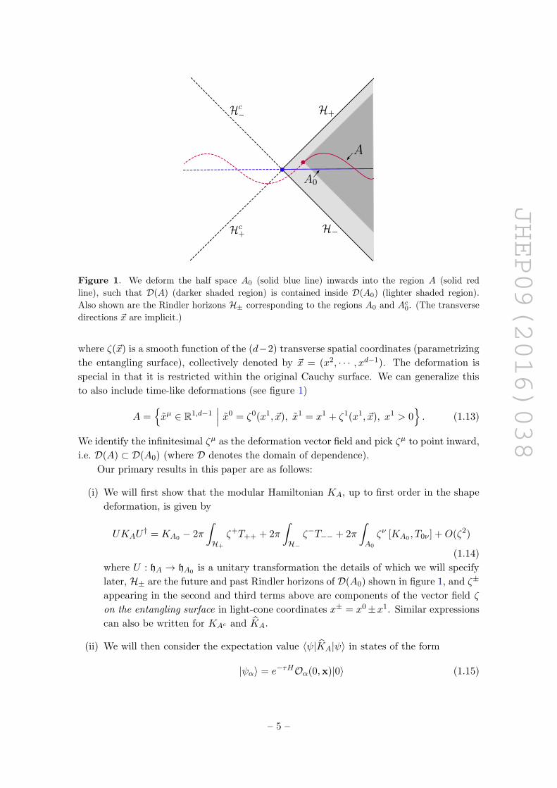
Figure 1. We deform the half space A0 (solid blue line) inwards into the region A (solid red

line), such that D(A) (darker shaded region) is contained inside D(A0) (lighter shaded region).

Also shown are the Rindler horizons H± corresponding to the regions A0 and Ac0. (The transverse

directions ~x are implicit.)

where ζ(~x) is a smooth function of the (d−2) transverse spatial coordinates (parametrizing

the entangling surface), collectively denoted by ~x = (x2, · · · , xd−1). The deformation is

special in that it is restricted within the original Cauchy surface. We can generalize this

to also include time-like deformations (see figure 1)

A ={xµ ∈ R1,d−1

∣∣∣ x0 = ζ0(x1, ~x), x1 = x1 + ζ1(x1, ~x), x1 > 0}. (1.13)

We identify the infinitesimal ζµ as the deformation vector field and pick ζµ to point inward,

i.e. D(A) ⊂ D(A0) (where D denotes the domain of dependence).

Our primary results in this paper are as follows:

(i) We will first show that the modular Hamiltonian KA, up to first order in the shape

deformation, is given by

UKAU† = KA0 − 2π

∫

H+

ζ+T++ + 2π

∫

H−ζ−T−− + 2π

∫

A0

ζν [KA0 , T0ν ] +O(ζ2)

(1.14)

where U : hA → hA0 is a unitary transformation the details of which we will specify

later, H± are the future and past Rindler horizons of D(A0) shown in figure 1, and ζ±

appearing in the second and third terms above are components of the vector field ζ

on the entangling surface in light-cone coordinates x± = x0±x1. Similar expressions

can also be written for KAc and KA.

(ii) We will then consider the expectation value 〈ψ|KA|ψ〉 in states of the form

|ψα〉 = e−τHOα(0,x)|0〉 (1.15)

– 5 –

JHEP09(2016)038

and linear combinations thereof, where H is the Hamiltonian and Oα is an arbitrary

local operator whose quantum numbers (dimension, spin etc.) are collectively denoted

by α.3 The factor of e−τH is added to make these states normalizable. In a CFT this

class of states is a basis for the entire Hilbert space, via the state-operator mapping.

For a general QFT similar statements should hold. In fact, there is no obstruction to

generalizing our argument to include states created by many local and even non-local

operators inserted throughout the lower half Euclidean plane. Further, we could also

insert the operators in real time. In the interest of simplifying our presentation we

choose to represent our state via a single operator insertion on the Euclidean section,

although we expect all our conclusions to go through even in the more general case.

We then show that equation (1.14), along with the positivity of the operator KA0−KA

(i.e. monotonicity under inclusion, which recall follows from the monotonicity of

relative entropy) implies the averaged null energy condition (ANEC)

∫ ∞

−∞dx+

⟨T++(x+, x− = 0, ~x)

⟩ψ≥ 0. (1.16)

As discussed in the introduction, the Hofman-Maldacena bounds on CFT three-

point functions were derived assuming the ANEC; so this completes the proof of

these bounds. It should perhaps be mentioned that the specific states considered

in deriving the HM bounds in [39] were created by inserting an approximately local

operator in real time, with an approximately specified four-momentum. Given our

remarks below equation (1.15), our derivation of the ANEC also applies to these

states.

(iii) Finally, we also discuss the (vacuum) full modular Hamiltonian for deformed half-

spaces in CFTs with classical gravity duals, which allows us to make contact with the

recent proposal by Jafferis-Lewkowyzc-Maldacena-Suh (JLMS) [6] for the holographic

dual to the modular Hamiltonian.

At this point we should mention that in continuum quantum field theory there are

significant ultraviolet (UV) issues associated with the definition of the reduced density

matrix for a region, often resulting in divergences for entanglement entropy and modular

energy which are local to the entangling surface. These issues and associated divergences

are however not present for quantities like the relative entropy, and the full modular Hamil-

tonian [47, 48]. Since this is ultimately what we are interested in, and in the interest of

simplicity of presentation, we will for the most part suppress the need for a UV cutoff at

the entangling surface. Indeed the answers we will find will be finite, partly justifying this

approach. For further discussion on how to include such a UV cutoff in our calculation, see

appendix A, where we will argue for the irrelevance of the details of such a cutoff beyond

its existence.

3In the case of tensor operators, we contract them with appropriate polarizations, for instance Oα(x) =

εµ1µ2···µsJµ1µ2···µs(x)

– 6 –

JHEP09(2016)038

2 Modular Hamiltonian for deformed half-space

In this section, we give an explicit formula for the modular Hamiltonian KA of the vacuum

state over a deformed half-space, to first order in the shape deformation.

2.1 Reduced density matrix

The vacuum state in a relativistic quantum field theory can be constructed by performing

the Euclidean path-integral over the region x0E < 0, where x0

E is Euclidean time. In the

interest of generality, let us instead consider a more general state rather than the vacuum4

|ψ〉 =∑

α

cα|ψα〉 = e−τH∑

α

cαOα(0,x)|0〉, · · · (τ > 0) (2.1)

This state can be constructed similarly as a sum over path-integrals, but with the operator

Oα inserted at x0E = −τ in the term proportional to cα. The reduced density matrix

corresponding to |ψ〉, associated with the undeformed half-space A0 is constructed as a

Euclidean path integral with specified field configurations above (x0E → 0+, x1 > 0) and

below (x0E → 0−, x1 > 0) the region A0 (see figure 2)

〈α0|ρψA0,η|β0〉 = N−1

A0,η

∫ φ+=β0

φ−=α0

[Dφ]η∑

α

∑

α′

c∗αcα′O†α(τ,x)Oα′(−τ,x) e−S[η,φ(x)] (2.2)

where we have collectively denoted all the fields integrated over in the path integral as φ,

and |α0〉, β0〉 ∈ hA0 are eigenstates of the field operator φ restricted to A0. The prefactor

N−1A0,η

is added to ensure the normalization of the density matrix, i.e. TrA0 ρψA0,η

= 1. We

have explicitly displayed the dependence of the reduced density matrix on the metric ηµν ,5

through the path integral measure (which we assume is diffeomorphism invariant), the

action and the normalization.

For convenience, we will henceforth use the notation (inside path-integrals)

X =∑

α

∑

α′

c∗αcα′O†α(τ,x)Oα′(−τ,x). (2.3)

Now consider the reduced density matrix over the deformed region A. This can be

constructed by a similar Euclidean path integral with specified field configurations above

and below A, and with a real-time fold around x0E = 0 in the case of time-like deformations

(ζ0 6= 0). We can deal with this path integral by performing a diffeomorphism f : xµ →xµ− ζµ, which maps A to A0. We can take ζµ to be non-vanishing (corresponding to non-

trivial f) only within a small region |x0E | < ` (for some ` � τ , but much larger than the

cutoff). Of course, such a diffeomorphism has a non-trivial action on the background metric

g = (f−1)∗η (2.4)

4Later, we will also need to compute the expectation value 〈KA〉ψ = TrA(ρψAKA,

)in the excited state

|ψ〉; so we derive the reduced density matrix ρψA along the way while setting up the calculation for KA.5Here by η we are denoting the metric in real time. Of course the corresponding metric on the Euclidean

section which is used in constructing the Euclidean path integral is δµν .

– 7 –

JHEP09(2016)038

x

xx0E

x1

x0E = ⌧

x0E = �⌧

O↵

O†↵

�+ = �0

�� = ↵0

Figure 2. The path integral construction for matrix elements of the reduced density matrix for

the state |ψα〉, over the original half space A0 (solid blue line). The operator insertions are marked

at x0E = ±τ . The black dot is the entangling surface (with transverse directions ~x implicit).

where ∗ denotes the pullback. We claim that the reduced density matrix over A (with the

metric η) is given by

ρψA,η = U † ρψA0,gU (2.5)

where U is a unitary transformation, and ρψA0,gis the reduced density matrix over the

undeformed half-space, but with the deformed metric g.

We now give a quick formal proof of this claim. If we denote the eigenstates of φ

restricted to A by |α〉, |β〉 · · · ∈ hA, then we can construct a unitary6 operator U : hA → hA0

given by

U =

∫[Dα]η |(f−1)∗α〉〈α| (2.6)

Then the claim (2.5) can be checked explicitly by a series of manipulations on the path-

integral definitions of the above density matrices [49]

〈α|ρψA,η|β〉 = N−1A,η

∫ φ+=β

φ−=α[Dφ]η X e−S[η,φ]

= N−1A,η

∫ (f∗φ)+=β

(f∗φ)−=α[D(f∗φ)]η X e−S[η,(f∗φ)]

= N−1A0,g

∫ φ+=(f−1)∗β

φ−=(f−1)∗α[Dφ]g X e−S[g,φ]

= 〈(f−1)∗α|ρψA0,g|(f−1)∗β〉

= 〈α|U †ρψA0,gU |β〉. (2.7)

6The unitarity follows from the diffeomorphism invariance of the measure: (f∗)∗ [Dα]η ≡ [D (f∗α0)]η =

[Dα0]g .

– 8 –

JHEP09(2016)038

The first equality follows from the definition of ρψA,η, the second equality is obtained by

changing variables φ = f∗φ inside the path integral, while the third equality follows from

the assumption that the measure is diffeomorphism invariant. We have throughout used

the fact that the operator insertions (denoted by X, following the definition (2.3)) are away

from the region where the diffeomorphism f has non-trivial support, and so f acts trivially

on these operators.

In the case where f is an infinitesimal diffeomorphism, we can obtain a perturbative

formula for ρψA0,g. Writing the deformed metric on the Euclidean section as

gµν = δµν + 2∂(µζν) +O(ζ2) (2.8)

where ζ is appropriately Wick rotated to Euclidean space, we obtain

UρψA,ηU† = ρψA0,η

+1

2

∫ddx δgµν(x)ρA0,η

{T (Tµν(x)X)

〈X〉 − 〈Tµν(x)X〉X〈X〉2

}+O(ζ2) (2.9)

where δgµν = 2∂(µζν), and T is the angular-ordering operator: if θ ∈ (0, 2π) is the angular

coordinate in the (x0E , x

1) plane, then

T (Oa(θa)Ob(θb)) = Oa(θa)Ob(θb)H(θa − θb) +Ob(θb)Oa(θa)H(θb − θa) (2.10)

where H is the Heaviside step function. For the special case |ψ〉 = |0〉, we then obtain

UρA,ηU† = ρA0,η +

1

2

∫ddx δgµν(x)ρA0,η

(Tµν(x)− 〈Tµν(x)〉

)+O(ζ2) (2.11)

2.2 Modular Hamiltonian

We are now in a position to construct the modular Hamiltonian over the deformed half-

space for the vacuum state

KA,η ≡ −ln ρA,η = −U † (ln ρA0,g)U = U †KA0,g U (2.12)

In order to perturbatively expand the right hand side in powers of ζ, we use the resol-

vent trick

− ln ρA0,g =

∫ ∞

0dλ

(1

ρA0,g + λ− 1

1 + λ

)(2.13)

which together with equation (2.11) gives

KA0,g = KA0,η + δζKA0 +O(ζ2) (2.14)

δζKA0 = −1

2

∫ ∞

0dλ

∫ddx δgµν(x) ρA0,η

1

ρA0,η + λ: Tµν : (x)

1

ρA0,η + λ(2.15)

where we have defined

: Tµν : (x) = Tµν(x)− 〈Tµν(x)〉. (2.16)

In the interest of simplifying notation, we will henceforth drop the explicit reference to

the Minkowski metric on ρA0,η, and simply refer to it as ρA0 . It is possible to perform

– 9 –

JHEP09(2016)038

x0E

x1

eR

Rb

@ eR+

@ eR�

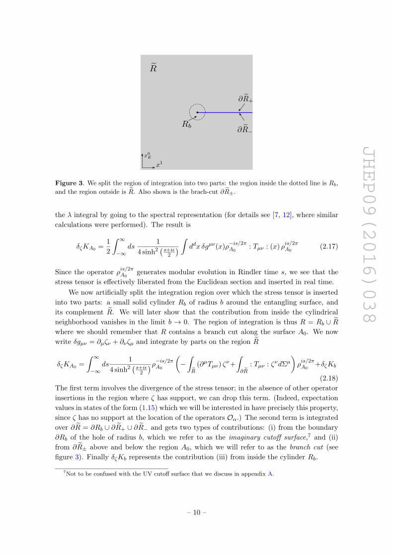
Figure 3. We split the region of integration into two parts: the region inside the dotted line is Rb,

and the region outside is R. Also shown is the brach-cut ∂R±.

the λ integral by going to the spectral representation (for details see [7, 12], where similar

calculations were performed). The result is

δζKA0 =1

2

∫ ∞

−∞ds

1

4 sinh2(s+iε

2

)∫ddx δgµν(x)ρ

−is/2πA0

: Tµν : (x) ρis/2πA0

(2.17)

Since the operator ρis/2πA0

generates modular evolution in Rindler time s, we see that the

stress tensor is effectively liberated from the Euclidean section and inserted in real time.

We now artificially split the integration region over which the stress tensor is inserted

into two parts: a small solid cylinder Rb of radius b around the entangling surface, and

its complement R. We will later show that the contribution from inside the cylindrical

neighborhood vanishes in the limit b → 0. The region of integration is thus R = Rb ∪ Rwhere we should remember that R contains a branch cut along the surface A0. We now

write δgµν = ∂µζν + ∂νζµ and integrate by parts on the region R

δζKA0 =

∫ ∞

−∞ds

1

4 sinh2(s+iε

2

)ρ−is/2πA0

(−∫

R(∂µTµν) ζν+

∫

∂R: Tµν : ζνdΣµ

)ρis/2πA0

+δζKb

(2.18)

The first term involves the divergence of the stress tensor; in the absence of other operator

insertions in the region where ζ has support, we can drop this term. (Indeed, expectation

values in states of the form (1.15) which we will be interested in have precisely this property,

since ζ has no support at the location of the operators Oα.) The second term is integrated

over ∂R = ∂Rb ∪ ∂R+ ∪ ∂R− and gets two types of contributions: (i) from the boundary

∂Rb of the hole of radius b, which we refer to as the imaginary cutoff surface,7 and (ii)

from ∂R± above and below the region A0, which we will refer to as the branch cut (see

figure 3). Finally δζKb represents the contribution (iii) from inside the cylinder Rb.

7Not to be confused with the UV cutoff surface that we discuss in appendix A.

– 10 –

JHEP09(2016)038

(i) Imaginary cutoff surface: let us first deal with the term supported on the surface

∂Rb. It is convenient to switch to complex coordinates

z = x1 − ix0E , z = −(x1 + ix0

E). (2.19)

In these coordinates, we find

ρ−is/2πA0

(ζµnνTµν(x)

)ρis/2πA0

=(− e2s−iθTzz(xs) + Tzz(xs)e

iθ)ζz (2.20)

+(− Tzz(xs)e−iθ + e−2s+iθTzz(xs)

)ζ z

where,

xµs = (b sin(θ + is), b cos(θ + is), ~x) (2.21)

Further, nν is the (inward pointing) unit normal to ∂Rb

n = eiθ∂z − e−iθ∂z. (2.22)

and ζz and ζ z are the components of the vector field ζ close to the entangling surface

in holomorphic coordinates

ζ = ζz∂z + ζ z∂z (2.23)

We now proceed by shifting the s integration contour s→ s+ iθ in order to remove

the θ dependence from the stress tensor. We do this after switching the order of

integration so that the s integral comes before the θ integral. This step assumes

analyticity in the complex s plane and that the contributions from s→ ±∞ vanish,

which can be justified in a spectral representation of (2.18). This gives

δζKA0 |∂Rb = − b∫dd−2~x

∫ 2π

0dθ

∫ ∞

−∞ds

1

4 sinh2(s+iθ

2

)

×(

(e2sTzz− : Tzz :)ζzeiθ + (: Tzz : −e−2sTzz)ζze−iθ

)(2.24)

where now these stress-tensors are evaluated at x0E = ib sinh(s), x1 = b cosh(s). We

can now perform the θ integral using

∫ 2π

0dθ

1

4 sinh2(s+iθ

2

)e±iθ = 2πe∓sΘ(±s)− 2πδ(s) (2.25)

The delta function term above can be dropped since this term does not contribute in

the limit b→ 0.8 So we get

δζKA0 |∂Rb = 2πb

∫dd−2~x

(−∫ ∞

0ds(esTzz − e−s : Tzz :)ζz

+

∫ 0

−∞ds(e−sTzz − es : Tzz :)ζ z

)(2.26)

8Actually, rather than drop this term, let us add it to a stack:

Stack = 2πb

∫dd−2~xT1µ ζ

µ.

We will update Stack everytime we find a term of this type in our calculation.

– 11 –

JHEP09(2016)038

Naively, it might seem that all the terms on the right hand side vanish in the b→ 0

limit. In fact, the terms involving Tzz do indeed vanish in this limit.9 However, the

terms involving Tzz and Tzz get an enhancement from the s integral, coming from the

s ∼ − ln b and s ∼ ln b limits respectively. Taking the limit b→ 0 and Wick rotating

the vector field back to real time, i.e. ζz → ζ+ and ζ z → ζ− (where the light-cone

coordinates are defined as x± = x0 ± x1), we obtain

δζKA0 |∂Rb = 2π

∫dd−2~x

(−∫ ∞

0dx+ζ+T++(x+, x− = 0, ~x)

+

∫ 0

−∞dx−ζ−T−−(x+ = 0, x−, ~x)

)(2.27)

where note that the first term on the right hand side is integrated over the future

Rindler horizon H+, while the second term is integrated over the past Rindler horizon

H−, shown in figure 1.

(ii) Branch cut : now we come to the second remaining term supported over ∂R+ ∪ ∂R−.

Once again, deforming the s contours to get rid of the θ dependence from the stress

tensors, we obtain

δζKA0 |∂R± =

∫dd−2~x

∫ ∞

bdx1

∫ ∞

−∞ds (2.28)

×(− 1

4 sinh2(s+iε

2

) +1

4 sinh2(s−iε

2

))tµζνρ−isA0

: Tµν : ρisA0

where t = ∂x0E

, and the stress tensor is evaluated on the region A0, i.e. Tµν ≡Tµν(x0

E = 0, x1, ~x) above. The first term inside the brackets comes from ∂R+ while

the second term comes from ∂R− (after the contour deformation s → s + 2π − 2ε).

It is clear from equation (2.28) that the s integral precisely picks out the double-pole

at s = 0. A straightforward application of the residue theorem gives

δζKA0 |∂R± = 2π

∫dd−2~x

∫ ∞

bdx1 tµζν

[Tµν(0, x1, ~x),KA0

](2.29)

(iii) Inside the hole: we can follow the same methods as in (i). Pick coordinates close to

the entangling surface such that:

ds2 = dr2 + r2dθ2 + d~x2 → dr2 − r2ds2 + d~x2 (2.30)

where we have also shown the Wick rotated Rindler coordinates. The hole region

Rb corresponds to r < b and since we are again working in a region close to the

9By this we mean that the Tzz terms do not contribute to matrix elements in the class of states (1.15)

which are of interest here. On the other hand, if we were to evaluate matrix elements in Rindler eigenstates

we would find potential divergences in this limit. Note that since we used a spectral representation for ρA0

at an intermediate stage, we were exactly evaluating this in Rindler eigenstates. So the order in which this

limit is taken is a somewhat delicate issue which is best ignored on a first pass. In appendix A we confront

this issue explicitly.

– 12 –

JHEP09(2016)038

entangling surface we can take the diffeomorphism at leading order to be independent

of r. After shifting the integration contour s→ s+ iθ and Wick rotating the ζ vector

field we have:

ρ−is+θ

2πA0

Tµν(x)∂µζνρis−θ2πA0

= eiθ+sTi+(x+, x−, ~x)∂iζ++e−iθ−sTi−(x+, x−, ~x)∂iζ

− (2.31)

The light-like coordinates where the stress tensor on the right hand side above is

located are x± = ±re±s. We still have to integrate (2.31) over:∫ddx

∫ds

1

4 sinh2(s+iθ

2

) . . . =

∫dd−2~x

∫

r<bdrr

∮dθ

∫ ∞

−∞ds

1

4 sinh2(s+iθ

2

) . . .

(2.32)

But at this point the θ dependence is the same as in (2.25) and we can again do the θ

integral. After ignoring the δ(s) contribution which vanishes in the limit b→ 0,10 this

has exactly the effect of switching the angular integral in the Euclidean calculation to

a real time integral localized near the Rindler horizon: 0 < r < b and −∞ < s <∞(see figure 4). The integrand is the stress tensor coupled to a real time diffeomorphism

of the metric

δζKb = 2π

∫

0<r<bddxTµν ∂

µζν (2.33)

for the following vector field:

ζ = Θ(x0)ζ+∂+ + Θ(−x0)ζ−∂− (2.34)

We have again ignored a contribution localized at x0 = 0, coming from the derivative

of the step functions above, which vanishes in the limit b→ 0.11

It is not hard to see that (2.33) should vanish in the limit b → 0. However it is

somewhat enlightening to go another route and instead integrate by parts on (2.33). We

get two terms, one from the r = b boundary and the other from precisely the past and

future Rindler horizons on the boundary of the domain of dependence of A0. It turns

out the former term cancels (2.26) prior to taking the b → 0 limit (although we always

need b small), and the later term is exactly the desired result given in (2.27) . So in

the end when we add all the terms together, no b → 0 limit is necessary and the null

10Once again, we add this term to the stack defined in footnote 8:

Stack→ Stack− 2π

∫dd−2~x

∫ b

0

dx1x1Tiµ∂iζµ.

11These terms go into the stack as well:

Stack → Stack + 2π

∫dd−2~x

∫ b

0

dx1(T10ζ0 + T00ζ

1)

= 2π

∫dd−2~x

∫ b

0

dx1 (x1∂0T0µζµ + 2T10ζ

0 + (T11 + T00)ζ1)where in the second equality we have integrated by parts; this is then exactly the extension of the x1 integral

in (2.29) so that it ranges from 0 to ∞. Even though all these terms vanish as b → 0, it is satisfying that

they add up like this.

– 13 –

JHEP09(2016)038

H+

H�

r = b

Figure 4. The contribution from inside the region Rb can be written in real time as an integral

over the shaded region.

energy operators in (2.27) simply emerge. This is perhaps not too surprising since the

r = b surface is imaginary, and there should be no dependence on b, however we find the

detailed cancelations that occur and the form in (2.33) intriguing (including in the running

footnote Stack), perhaps hinting that there is a different way to do this calculation directly

in real times.

To summarize, putting everything together, we find that the modular Hamiltonian

over the deformed half-space is given by

UKAU† = KA0 − 2π

∫

H+

ζ+T++ + 2π

∫

H−ζ−T−− + 2π

∫

A0

tµζν [Tµν ,KA0 ] (2.35)

which is the result claimed in (1.14).12 We emphasize once again that the ζ± appearing in

the second and third terms above are defined at the entangling surface and in particular

do not depend on the null coordinates x± along the Rindler horizons. We can also derive

a similar expression for the modular Hamiltonian corresponding to the complement Ac

V KAcV† = KAc0

+ 2π

∫

Hc+ζ+T++ − 2π

∫

Hc−ζ−T−− + 2π

∫

A0ctµζν

[Tµν ,KAc0

](2.36)

whereHc± are the Rindler horizons corresponding to the complement Ac0, and V : hAc → hAc0is a unitary transformation. Finally, putting these together, we obtain the following formula

for the full modular Hamiltonian

UKAU† = KA0 − 2π

∫

L+

ζ+T++ + 2π

∫

L−ζ−T−− + 2π

∫

Σtµζν

[Tµν , KA0

](2.37)

where we have defined the light sheets L± = H± ∪ Hc±, and U : hΣ → hΣ is a unitary

transformation given by U = U ⊗ V .

12Roughly speaking, the “null-energy” terms measure the amount of modular energy leaving the Rindler

wedge, while the commutator term comes from the action of the unitary transformations on the original

(undeformed) modular Hamiltonian.

– 14 –

JHEP09(2016)038

3 Averaged null energy condition

In this section, we will consider the expectation value 〈ψ|KA|ψ〉 in the class of states (1.15).

We will then use the positivity of the operator KA0− KA to prove the averaged null energy

condition within this class.

3.1 Positivity of KA0 − KA

For completeness, we begin with a brief review of the argument that KA0−KA is a positive

operator, following [22].13 Consider any two states, which we take here to be the vacuum

|0〉 and a non-trivial pure state |ψ〉. Given an entangling region A0 and the corresponding

reduced density matrices ρA0 and ρψA0, one defines the relative entropy

S(ρψA0||ρA0) = TrA0

(ρψA0

ln ρψA0

)− TrA0

(ρψA0

ln ρA0

)(3.1)

=[TrA0

(ρψA0

KA0

)− TrA0 (ρA0 KA0)

]

+[TrA0

(ρψA0

ln ρψA0

)− TrA0 (ρA0 ln ρA0)

]

≡ ∆〈KA0〉 −∆SEE[A0]. (3.2)

where KA0 is the modular Hamiltonian corresponding to the vacuum state over the re-

gion A0.

Relative entropy has a number of interesting properties. For instance, it is a posi-

tive quantity

S(ρψA0||ρA0) ≥ 0 (3.3)

Further, if we pick another region A such that A ⊂ A0 (more precisely, if D(A) ⊂D(A0), where D(A) is the domain of dependence of A) then the monotonicity of relative

entropy implies

S(ρψA||ρA) ≤ S(ρψA0||ρA0) (3.4)

Intuitively, the relative entropy measures the distinguishability between two states. From

this point of view, the monotonicity property states that the distinguishability between

two states decreases as we consider their reduced density matrices over smaller and

smaller regions.14

From equations (3.2) and (3.4), we obtain

∆ 〈KA〉 −∆ 〈KA0〉 −∆SEE[A] + ∆SEE[A0] ≤ 0 (3.5)

∆⟨KAc0

⟩−∆ 〈KAc〉 −∆SEE[Ac0] + ∆SEE[Ac] ≤ 0 (3.6)

where all modular Hamiltonians are defined relative to the vacuum. Adding the two in-

equalities we have

∆⟨KA

⟩−∆

⟨KA0

⟩−∆SEE[A] + ∆SEE[A0]−∆SEE[Ac0] + ∆SEE[Ac] ≤ 0 (3.7)

13Similar arguments have been used in [4, 50]. A rigorous proof of the positivity of this operator can also

be found in [21] which uses methods of algebraic QFT.14See [51–53] for field theoretic calculations of relative entropy in excited states, using a version of the

replica trick.

– 15 –

JHEP09(2016)038

Now, since all vacuum contributions vanish, we can drop the ∆. (This is because KA

annihilates the vacuum for any region A). This implies

⟨KA

⟩ψ−⟨KA0

⟩ψ≤ SEE[ψ,A]− SEE[ψ,Ac]− SEE[ψ,A0] + SEE[ψ,Ac0] = 0 (3.8)

where the last equality follows from the purity of |ψ〉. Since this is true for any pure state

|ψ〉, we deduce that KA0 − KA is a positive operator.

3.2 Computing 〈KA0〉ψ − 〈KA〉ψWe now explicitly compute the expectation value of KA0 − KA in the state

|ψ〉 = e−τH∑

α

cαOα(0,x)|0〉 (3.9)

where as before we take A0 to be the half-space x1 > 0, and A to be the deformed half-space.

Using the relation

〈ψ|KA|ψ〉 = TrA

(ρψAKA

)− TrAc

(ρψAcKAc

)(3.10)

we find

〈ψ|(KA0 − KA)|ψ〉 = T(1) + T(2) (3.11)

where

T(1) = −TrA0

(δζρ

ψA0KA0

)+ TrA0

c

(δζρ

ψA0

cKAc0

)(3.12)

T(2) = −TrA0

(ρψA0

δζKA0

)+ TrA0

c

(ρψA0

cδζKAc0

)(3.13)

where note that the unitary transformations U and V have dropped out inside the trace.

The second term above is straightforward to evaluate from equations (2.35) and (2.36):

T(2) = 2π

∫

L+

ζ+〈T++〉ψ − 2π

∫

L−ζ−〈T−−〉ψ + 2π

∫

Σtµζν〈

[KA0 , Tµν

]〉ψ (3.14)

where we have defined

〈Y 〉ψ ≡〈ψ|Y |ψ〉〈ψ|ψ〉 . (3.15)

The first two terms in (3.14) are the appropriate null energy expectation values (albeit

integrated along the transverse ~x directions with arbitrary coefficients ζ±(~x)) which enter

in the averaged null energy condition. We will see below that the last term in (3.14) is

precisely cancelled by a contribution coming from T(1).

Consider for instance, the first term in T(1); from equations (2.9) and (3.12) we obtain

TrA0

(δζρ

ψA0KA0

)=

1

2

∫

Rδgµν(x)

{〈Tµν(x)KA0X〉〈X〉 − 〈T

µν(x)X〉〈KA0X〉〈X〉2

}(3.16)

On the right hand side, the correlators 〈· · · 〉 indicate Euclidean correlation functions on

Rd, and recall the notation

X =∑

α

∑

α′

c∗αcα′O†α(τ,x)Oα′(−τ,x). (3.17)

– 16 –

JHEP09(2016)038

Note that the Euclidean correlation function appears naturally from the path integral

construction of the deformed density matrix for the excited state — we need only add an

insertion of KA0 along A0 and trace — resulting in the above correlation function. Because

of the KA0 operator insertion, we should remove an infinitesimal cut running along A0 from

the region over which we integrate the diffeomorphism R. Bearing this in mind, we can

integrate by parts in the region R to obtain only a contribution from above and below the

KA0 operator insertion, yielding a commutator:

TrA0

(δζρ

ψA0KA0

)= −2π

∫

Σdd−2~x

∫ ∞

0dx1 ζµtν

⟨[KA0 , T

µν(0, x1, ~x)]⟩ψ

(3.18)

where we reiterate that ζ vanishes at the locations of the operators Oα, which allows us to

drop the divergence of the stress tensor. For the full modular Hamiltonian we then have:

T(1) = −2π

∫

Σdd−2~x

∫ ∞

−∞dx1 ζµtν

⟨[KA0 , T

µν(0, x1, ~x)]⟩ψ

(3.19)

As promised, this term precisely cancels the last term in equation (3.14). We therefore

conclude that

〈KA0〉ψ − 〈KA〉ψ = 2π

∫

L+

ζ+〈T++〉ψ − 2π

∫

L−ζ−〈T−−〉ψ (3.20)

Since ζ+ > 0 and ζ− < 0 by construction (see figure 1), the positivity of the operator

(KA0 − KA) leads to the averaged null energy conditions

∫ ∞

−∞dx+

⟨T++(x+, x− = 0, ~x)

⟩ψ≥ 0,

∫ ∞

−∞dx−

⟨T−−(x+ = 0, x−, ~x)

⟩ψ≥ 0 (3.21)

This concludes our proof that the monotonicity property of KA implies the ANEC. While

we presented the proof above in the context of half-spaces in Minkowski space-time, the

above calculation can also be extended in an obvious way to general static bifurcate Killing

horizons. In this case we would be studying the modular Hamiltonian for small deforma-

tions of the entangling cut away from the bifurcation point in the Hartle-Hawking state.

The monotonicity constraint then leads to the ANEC for complete null generators of the

Killing horizon.

4 Modular Hamiltonians in AdS/CFT

In this section we make a connection between our results and the recently proposed JLMS

formula [6]:

KCFTA =

Area∂M\A

4GN+Kbulk

M + · · ·+O(GN ) (4.1)

where A denotes the boundary subsystem, and M denotes the bulk region enclosed by

the minimal/extremal Ryu-Takayanagi/HRT [54, 55] surface ∂M\A (which ends on the

– 17 –

JHEP09(2016)038

entangling surface ∂A, and is homologous to A). Further, the · · · denote local terms on the

extremal surface, which will not be relevant in the following discussion. The result (4.1)

arises as a consequence of the formula for quantum corrections to the Ryu-Takaynagi

entropy [56, 57] (see also [58].)

Here, we want to perform a simple consistency check of our formula (2.37) for the

full modular Hamiltonian of deformed half-spaces against equation (4.1). In particular,

restricting to pure states so that the bulk area operator Area∂M\A evaluates the same over

A and Ac, (4.1) allows us to equate the full modular energies between the boundary and

the bulk theories

KCFTA = Kbulk

M +O(GN ) (4.2)

where note that the local terms on the extremal surface have also dropped out.

In order to make contact with our previous results, we take A to be a small deformation

of the boundary half-space A0 = {x1 > 0, x0 = 0}. If we use the coordinates(z, x0, x1, ~x

)

on the Poincare patch of AdS, with

gAdS =dz2 − (dx0)2 + (dx1)2 + (d~x)2

z2, (4.3)

then the corresponding (undeformed) extremal surface in the bulk is given by the codi-

mension two surface x0 = x1 = 0, and we have the corresponding undeformed region

M0 = {x1 > 0, x0 = 0}. To linear order in the CFT shape deformation ζ, we then expect

〈δζKCFTA0〉ψCFT

= 〈δζbulkKbulkM0〉ψbulk

+O(GN ), (4.4)

where we have evaluated the deformations in the CFT and bulk modular Hamiltonians in

an excited boundary state |ψ〉CFT and the dual bulk state |ψ〉bulk respectively. Further,

ζbulk is the deformation in the bulk minimal surface as a consequence of the boundary shape

deformation, and approaches ζ in the limit z → 0; it is fixed away from the boundary by

the requirement that the deformed bulk surface remain extremal [55].

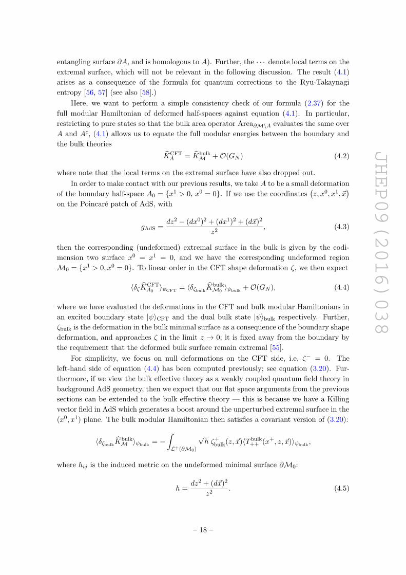
For simplicity, we focus on null deformations on the CFT side, i.e. ζ− = 0. The

left-hand side of equation (4.4) has been computed previously; see equation (3.20). Fur-

thermore, if we view the bulk effective theory as a weakly coupled quantum field theory in

background AdS geometry, then we expect that our flat space arguments from the previous

sections can be extended to the bulk effective theory — this is because we have a Killing

vector field in AdS which generates a boost around the unperturbed extremal surface in the

(x0, x1) plane. The bulk modular Hamiltonian then satisfies a covariant version of (3.20):

〈δζbulkKbulkM 〉ψbulk

= −∫

L+(∂M0)

√h ζ+

bulk(z, ~x)〈T bulk++ (x+, z, ~x)〉ψbulk

,

where hij is the induced metric on the undeformed minimal surface ∂M0:

h =dz2 + (d~x)2

z2. (4.5)

– 18 –

JHEP09(2016)038

A consequence of JLMS combined with our calculations is therefore:∫

L+(∂A0)dd−2~xdx+ ζ+〈ψCFT|TCFT

++ |ψCFT〉

=

∫

L+(∂M0)

√hdd−2~xdx+dz ζ+

bulk〈ψbulk|T bulk++ |ψbulk〉 (4.6)

Our goal now is to establish this equivalence using the usual rules of AdS/CFT [59–61]. In

particular in order to apply the JMLS argument the state under consideration must have

a perturbative in GN back-reaction on the bulk AdS space-time and so we will consider

boundary states of the form |ψCFT〉 = O(xψ)|0〉CFT, where O is a single trace primary

scalar operator of dimension ∆ = O(1) in terms of large-N counting. The operator is

inserted at xψ : (x0ψ = −iτ, x1

ψ = 0, ~xψ = 0). In this case the dual bulk state can be

identified as |ψbulk〉 = limz→0 z−∆φ(z, xψ)|0〉AdS for the corresponding bulk field φ. The

equality in (4.6) can already be read off from the work of Hofman and Maldacena [39] but

here, for completeness, we will give another derivation.

For a CFT with a weakly coupled Einstein gravity dual in the bulk, the l.h.s. can be

computed using Witten diagrams. In particular, we assume that the relevant part of the

bulk Lagrangian takes the form:

Sbulk ∼∫

AdSd+1

√G

[− 1

GN(RG + Λ) +

1

2Gµν∂µφ∂νφ−m2

∆φ2

], m2

∆ = ∆(∆− d) (4.7)

The leading order Witten diagram contribution to the l.h.s. of (4.6) comes from the coupling

between the graviton (hµν = δGµν) and the scalar stress tensor:

Lbulkint =

√GhµνT bulk

µν (φ) (4.8)

where T bulkµν (φ) = ∂µφ∂νφ − 1

2Gµν∂αφ∂αφ + 1

2Gµνm2∆φ

2 is the leading order bulk stress

tensor in O(1/N). We thus have for the integrand:

〈O†(x?ψ)TCFT++ (x)O(xψ)〉 =

∫dzddx′

√GDµν

++(z, x′;x) (4.9)

×{∂µD

φ(z, x′;xψ)∂νDφ(z, x′;x?ψ) + . . .

}

=

∫dzddy

√GDµν

++(z, x′;x)T bulkµν

(Dφ(z, x′;xψ)

)(4.10)

where Dµναβ(z, x′;x) and Dφ(z, x′;xψ) are the bulk-to-boundary propagators for the graviton

and scalar respectively. We identify the products of scalar boundary-to-bulk propagators

as giving rise to the expectation value of the bulk stress tensor in the state |ψ〉bulk:

T bulk(Dφ(z, x′;xψ)

)= 〈T bulk

µν (z, x′)〉ψbulk(4.11)

To see this, we focus on a particular term ∂µφ∂νφ in T bulkµν (φ). When viewed as a bulk

operator, its expectation value in the bulk state |ψbulk〉 is given by:

〈∂µφ(z, x′)∂νφ(z, x′)〉ψbulk= lim

ε,ε′→0ε−∆ε′−∆〈φ(ε, x?ψ)∂µφ(z, x′)∂νφ(z, x′)φ(ε, xψ)〉 (4.12)

– 19 –

JHEP09(2016)038

The leading order (disconnected) diagram of the bulk 4-point function is given by products

of bulk-to-bulk propagator:15

〈φ(ε, x?ψ)∂µφ(z, x′)∂νφ(z, x′)φ(ε, xψ)〉= ∂µ〈φ(ε, x?ψ)φ(z, x′)〉∂ν〈φ(z, x′)φ(ε′, xψ)〉

= ∂µDφbulk-to-bulk(ε, x?ψ; z, x′)∂νD

φbulk-to-bulk(z, x′; ε′, xψ)

The boundary-to-bulk and bulk-to-bulk propagators are related by the limit:

Dφ(z, x′;x) = limε→0

ε−∆Dφbulk-to-bulk(z, x′; ε, x) (4.13)

We thus see that ∂µDφ(z, x′;x?ψ)∂νD

φ(z, x′;xψ) = 〈∂µφ(z, x′)∂νφ(z, x′)〉ψbulk. Similar rela-

tions hold for the other two terms in T bulkµν and we conclude that:

〈O†(x?ψ)TCFT++ (x+, xi)O(xψ)〉 =

∫dzddx′

√GDµν

++(z, x′;x)〈T bulkµν (z, x′)〉ψbulk

(4.14)

We need to integrate this relation over∫dx+dd−2~xζ+(xi) on the boundary. In particular,

since ζ+(~x) is independent of x+, we can take it out of the null integral, and replace∫dx+Dµν

++(z, x′;x+, ~x) = δµν++Dshock(z, ~x′; ~x)δ(x′−), where Dshock(z, ~x′; ~x) is the boundary-

to-bulk propagator for the shock wave graviton mode: h++(z, x′−, ~x) = f(z, ~x′)δ(x′−).

In AdSd+1, Dshock(z, ~x′; ~x) is determined by solving Einstein’s equations for this metric

fluctuation giving the shock-wave equation:16

(∂2z + ∂2

i −d+3

z∂z +

2d+4

z2

)Dshock(z, yi;xi) = 0, lim

ε→0Dshock(ε, yi;xi)→ ε2δd−2(xi − yi)

(4.15)

The factor δµν++δ(x′−) localizes the bulk integral onto L+(∂M0), and projects onto the

(++) component of bulk stress tensor:

∫

L+(∂A0)ζ+(xi)〈TCFT

++ (x+, xi)〉ψCFT=

∫

L+(∂M0)

√hζ+(z, ~x′)〈T bulk

++ (z, x′− = 0, x′+, ~x′)〉ψbulk

ζ+(z, ~x′) = z−2

∫dd−2~xζ+(~x)Dshock(z, ~x′; ~x) (4.16)

One can finally check from (4.15) that ζ+(z, ~x′) satisfies the extremal bulk extension of

ζ+(~x) on ∂M(A0):

(−d− 1

z∂z + ∂2

z + ∂2~x′

)ζ+(z, ~x′) = 0, lim

ε→0ζ+(ε, ~x′)→ ζ+(~x′) (4.17)

which is precisely what defines ζ+bulk(z, ~x), making (4.16) equivalent to (4.6), consistent

with JLMS formula.

15We analytically continue these propagators to real time such that the ordering is the appropriate one

for computing expectation values in the state |ψ〉bulk.16This shock wave metric is actually a full non-linear solution to Einstein’s equations although we have

not used this fact.

– 20 –

JHEP09(2016)038

5 Discussion

In this paper, following the circle of ideas in [16, 22, 50], we established a relation between

the monotonicity of relative entropy and the averaged null energy condition in arbitrary

QFTs, and in so doing proved the most general Hofman-Maldacena bounds on the data

in CFT three-point functions. We will now summarize the perturbative calculation we

performed to establish this connection and then conclude with possible future work.

The general goal was to study perturbatively the shape dependence of modular Hamil-

tonians/energies. We did this by applying “perturbation theory for reduced density ma-

trices” which turns out to have some novel features which we describe now. Schematically

the important term in our calculation (2.15) came from expanding the log used to define

the modular Hamiltonian. Here we give an alternative description of this expansion:

− ln ρA0(1 + ρ−1A0δρ) = KA0 −

∞∑

n=0

(−1)nBnn!

[KA0 ,

[KA0 , . . .

[KA0 , ρ

−1A0δρ]]]

︸ ︷︷ ︸n−times

+O(δρ2) (5.1)

where Bn are the Bernoulli numbers. The right hand side comes about due to the non

commutativity of the two matrices in the log on the left hand side. That is, these are the

usual nested commutator terms in the Baker-Campbell-Hausdorff formula keeping only

terms to order O(δρ) (see also [62] for related discussion).

This set of nested commutators clearly has something to do with the evolution with

respect to KA0 - or in other words modular flow. So it should come as no surprise that

these terms can be re-summed into an integral over ρ−is/2πA0

(ρ−1A0δρ)ρis/2πA0

multiplied by

some kernel - a fact we used in (2.17). In fact, in going from equation (5.1) to (2.17), one

simply uses the following integral representation of the Bernoulli numbers [63, 64]:17

Bn = −(−i)n(2π)n

∫ ∞

−∞ds

sn

4 sinh2( s+iε2 )· · · (n ∈ Z). (5.2)

Surprisingly this integral and kernel as well have the effect of switching the original Eu-

clidean diffeomorphism contained in δρ and used to move around the entangling surface,

to a real time diffeomorphism determined by the new vector field given in (2.33). From

here the null energy operators involved in the ANEC just pop out as boundary terms when

integrating by parts over the real time diffeomorphism. Of course in real times now a new

boundary has opened up; what previously was the co-dimension 2 entangling surface at

the origin in Euclidean space becomes a null hypersurface along the Rindler horizon where

the null energy operators are defined.

The non-commutativity emphasized in (5.1) was of fundamental importance to our

calculation. We feel that we do not fully understand the magic behind this calculation and

that there are new surprises lurking if we go to higher orders in perturbation theory and try

to systematize this approach. Similar tools were applied in [7, 12] to entanglement entropy

17Note that we pick the convention where B1 = + 12; also recall that B2m+1 = 0 for m = 1, 2 · · · .

The corresponding terms in the integral representation (5.2) pick out the residue at s = 0, which is only

non-trivial for n = 1.

– 21 –

JHEP09(2016)038

where it was important to control these commutator terms in order to find agreement

between this perturbative approach and known results from AdS/CFT. Here we have also

established a similar agreement with AdS/CFT and in particular the recent proposal by

JLMS [6] for the modular Hamiltonian in AdS/CFT.

Apart from gaining a deeper understanding into the inner working of these calculations

we now give some detail of future work that we think would be valuable to pursue.

5.1 Sharpening the argument

In the main sections of the paper our derivation eschewed any issues related to the precise

definition of entanglement and modular energy in quantum field theory. Indeed these

quantities are expected to be afflicted by significant UV divergences, and possibly even

ambiguities related to how one splits the degrees of freedom between A and Ac. Thus

in order to calculate these quantities we must specify a regulator and a prescription for

splitting the Hilbert space. However it became clear to us that we never needed to do this,

and so any real discussion of a regulator was relegated to appendix A.

Ultimately this should not have come as a surprise, the final goal was to calculate

either relative entropy or the full modular Hamiltonian - both of which are expected to be

UV finite quantities and both of which can actually be given a definition directly in the

continuum [47, 48]. This definition however was not convenient for our current calculation

so at an intermediate step we needed to calculate the expectation of the full modular

Hamiltonian in terms of the UV sensitive (half) modular Hamiltonian. Since we never

explicitly saw these UV divergences, our manipulations should be regarded as formal.18

Appendix A is an attempt to remedy this, by giving some details of a brick wall like

regulator [66] that renders the modular energy and associated quantities well-defined. The

brick wall regulator introduces dependence on the boundary conditions one chooses for

fields at the wall close to the entangling surface.

The regulated version of relative entropy does not satisfy the property of monotonicity

(for a finite but small cutoff scale) since the brick wall cutoff is a rather drastic modification

to the theory that does not allow one to compare different spatial regions with the same

modification. So to claim a completely rigorous proof of the ANEC we still need to show

that when we remove the brick wall cutoff the quantity we get is the continuum version of

relative entropy - which is then known to be monotonic [47]. This requires methods that

are beyond the scope of this paper, and we leave this to future investigations. Ultimately

we would like a mathematically rigorous derivation, perhaps without reference to density

matrices and using methods of algebraic quantum field theory [21, 48].

Finally we would like to understand if there are any restrictions on the state in which

we calculate the expectation value of the deformed modular Hamiltonian. For example

we formulated our state in terms of a local operator insertion at x0E = ±τ , which is

sufficiently general for a CFT. More generally, say for relativistic theories, our argument

will go through relatively unmodified if we just insert a general state of the theory and

18They might be regarded as about as formal as the usual derivation of the replica trick for Renyi entropies

in terms of a partition function on a singular surface [65].

– 22 –

JHEP09(2016)038

its conjugate in flat space along the Euclidean time slices x0E = ±τ . However we are

required to separate the diffeomorphism that moves around the entangling surface away

from |x0E | ≥ τ . We can make the region in which the diffeomorphism acts small but we

should be limited by |ζ| the size of the diffeomorphism vector field at the entangling surface.

This presumably puts some restriction on the state such that the expectation value of the

stress tensor cannot get arbitrarily large. For example if we work with the state created by

a local operator insertion |∫H± 〈T±±〉ψ | ∼ τ−1 < |ζ|−1. This is likely just the restriction

that the perturbative expansion converge and we can always arrange this to happen by

taking a small enough spatial deformation.

5.2 Generalizations

One obvious generalization involves attempting to prove the ANEC in other space-times as

well as along more general complete achronal null geodesics.19 Along these lines it might

be an easier first step to try to apply the methods of this paper to stationary but not

static black holes with the null generator lying along a bifurcate Killing horizon (like the

Kerr black hole). Since we used the framework of perturbation theory starting from a state

described by a known density matrix (the Hartle-Hawking state) we are not very optimistic

this will succeed when we don’t have such a starting point.

Instead perhaps a more fruitful direction to pursue would be to consider the generalized

second law (GSL) for quantum fields outside of a black hole with a static bifurcate Killing

horizon. Here we are referring to the work of [16] where the GSL was proven for free as well

as super renormalizable QFTs.20 The GSL applies to the following generalized entropy:

Sgen =Area(∂A)

4GN+ SEE(ρψA) (5.3)

where Area(∂A) refers to the area of a codimension-1 slice of the Killing horizon where

the spatial region A ends (∂A) and SEE is the entanglement entropy of the quantum

fields outside this horizon slice. Applying the monotonicty of relative entropy to SEE(ρψA)

one finds:

∆Sgen ≥∆Area(∂A)

4GN+ ∆ 〈KA〉ψ (5.4)

where now ∆ is a finite null deformation (∆x+ = ζ+(~y)) of the entangling surface ∂A

to the future of the bifurcation surface ∂A0. The change in the area is simply due to the

perturbative back reaction of the quantum fields on the space-time via Einstein’s equations:

∆Sgen ≥ 2π

∫dd−2~x

(−∫ ∞

ζ+

dx+(x+ − ζ+) 〈T++〉ψ +

∫ ∞

0dx+x+ 〈T++〉ψ

)+ ∆ 〈KA〉ψ

(5.5)

19These are geodesics where no two points on the curve are timelike separated. The ANEC is known to

fail in curved space-times where the null geodesic is chronal [37, 67].20The Hawking area theorem proves the GSL when the area term dominates in the GN → 0 limit - that

is for a classical dynamical background where the classical matter satisfies the NEC. As discussed in [16],

what remains, is to prove the GSL when classically the area does not increase - for quantum fields on a

stationary black hole background plus free gravitons. For obvious reasons here we then focus on the static

case, and leave out gravitons for simplicity.

– 23 –

JHEP09(2016)038

where we have made use of the Raychaudhuri equation with the correct future boundary

condition appropriate for a causal horizon.

To make further progress we need some handle on KA for general null deformations

away from A0. This does not sound very promising for our perturbative approach, however

it does seem like we can carry out our calculations to arbitrary orders in ζ+ [68]. Thus

with some luck we might be able to prove a statement about KA and get a handle on (5.5)

and possibly show the GSL in this case, ∆Sgen ≥ 0. A further hint comes actually from

AdS/CFT. For a Rindler space cut we have carried out a more detailed calculation21

than that outlined in section 4 where we previously showed the equality between the null

energy operators in the bulk and boundary. More generally one can show for finite null

deformations, but small perturbations to the state (in the 1/N sense):

2π

∫dd−2~x

∫ ∞

ζ+

dx+(x+ − ζ+

) ⟨TCFT

++

⟩ψ

=Area∂M\A(δg)

4GN+ 2π

∫dd−2~x

√h

∫ ∞

ζ+bulk

dx+(x+ − ζ+

bulk

) ⟨Tmatter

++

⟩ψ

(5.6)

and our notation is the same as that in section 4, where for example ζ+bulk is the bulk

HRT extremal surface corresponding to the deformation ζ+ on the boundary andM is the

spatial region between this extremal surface and A on the boundary. Here the area term

is the change in the area of the extremal surface due to the backreaction on the metric δg

in the state ψ (via Einstein’s equations.) Note that the extremal surface condition in pure

AdS for finite null deformations remains a linear differential equation that matches with

the infinitesimal version (4.17) and so ζ+bulk is the same extension as that used in section 4.

Now comparing this statement with that of JLMS [6] we could consistently identify the

modular Hamiltonian for finite null deformed regions as:

KCFTA

?= 2π

∫dd−2~x

∫ ∞

ζ+

dx+(x+ − ζ+

)TCFT

++ (5.7)

up to an additive constant, with a similar equation holding for the bulk region modular

Hamiltonian KbulkM . This is certainly not a proof. We have made two guesses (for the

bulk and the boundary) and shown them to be self-consistent. And in particular this only

works for a special class of states that don’t have a large back reaction on the bulk. Note

that this last issue also plagued our comparison between the bulk and boundary for small

deformations. We simply note here that our perturbative approach, when considered at

higher orders, can possibly prove such a statement.22 Of course if (5.7) is true then the

GSL follows trivially since the right hand side of the inequality in (5.5) just vanishes.

21This calculation has some overlap with [69] and the details will be reported elsewhere.22Actually a simpler argument is to take the perturbative result we have derived for null shape deforma-

tions and then use the QFT boost generator around the original undeformed Rindler cut to amplify the

deformation. This boost will then act on the state. However if we work in a sufficiently general state this

should not matter. This process seems to work, and agrees with (5.7), when trying to construct the full

modular Hamiltonian and we leave the details of how this works for the half space modular Hamiltonian

for the future. We thank Aron Wall for suggesting this argument to us.

– 24 –

JHEP09(2016)038

Finally we point out that in some sense these calculations have already been pushed to

higher orders. Rather than consider the excited state modular energy, if we just calculate

the modular Hamiltonian in the original vacuum state it should reproduce the entropy of

the vacuum. At first order this vanishes but the second order variation of entropy in a

CFT was calculated in [7] using similar methods to this paper. This quantity is sometimes

referred to as entanglement density [70]. Although it was not realized at the time the answer

in [7] can be related to a correlation function of two “null energy operators” - the same null

energy operators that appear in the (half sided) modular Hamiltonian in this work. This

will be the subject of a forthcoming paper [71]. Taken together this hints at a unifying

picture for vacuum entanglement in CFTs related to null energy operators that may even

pave the way to a new understanding and proof of the Ryu-Takayanagi [54] and HRT [55]

proposals for calculating entanglement entropy in the vacuum state of holographic CFTs.

Acknowledgments

It is a pleasure to thank Xi Dong, Gary Horowitz, Veronika Hubeny, Aitor Lewkowycz,

Don Marolf, Mukund Rangamani, David Simmons-Duffin and Aron Wall for discussions

and suggestions. Work supported in part by the U.S. Department of Energy contract

DE-FG02-13ER42001 and DARPA YFA contract D15AP00108.

A Cutoff at the entangling surface

In this appendix we would like to give a prescription for regulating the modular energy

that we calculate in the main part of the paper. We go through this in some depth because

the arguments we gave previously were somewhat formal. Although the quantity in which

we are ultimately interested — the full modular Hamiltonian — is UV finite [48], at inter-

mediate steps we encountered quantities which are not. In particular the modular energy

of some state is expected to have the same UV divergences as the entanglement entropy of

that state because the difference between them is the relative entropy which is UV finite.23

Thus the issues here are the same as the usual issues of defining entanglement entropy

in the continuum.24 There are several ways to define a regulated version of entanglement

entropy, but the most convenient for us will be a “brick wall” regulator [66]. This is so we

can still use Euclidean path integral methods to construct the density matrices in question.

Apart from possible IR issues the entropies are now finite - the IR issues do not concern

us and cancel when evaluating the differences between excited and vacuum states, at least

for states that are sufficiently close to the vacuum near the boundaries of space.

23There are still several reasons to expect some of our intermediate steps to be finite. Any divergences

should be local to the entangling surface, and assuming our regulator is geometric[72–74] no such term

which respects the S(A) = S(Ac) purity condition can generate a divergence for first order spatial shape

deformations. Similarly there is a general expectation that any such divergences cancel in the difference

S(ρψA) − S(ρA) although we will find evidence that this cancellation might not always occur. Of course

these variations and differences are still calculated in terms of divergent quantities so we proceed.24For a recent discussion of some of the issues involved see [72, 75]. When the QFT in question is a gauge

theory there are even questions about how the degrees of freedom are split between two spatial regions [76].

– 25 –

JHEP09(2016)038

x

xx0E

x1

r = b

r = a

O↵

O†↵

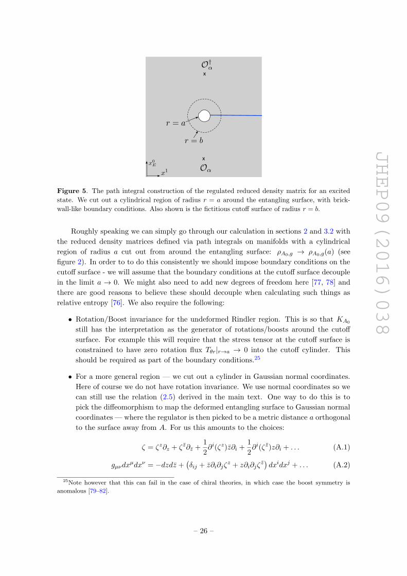
Figure 5. The path integral construction of the regulated reduced density matrix for an excited

state. We cut out a cylindrical region of radius r = a around the entangling surface, with brick-

wall-like boundary conditions. Also shown is the fictitious cutoff surface of radius r = b.

Roughly speaking we can simply go through our calculation in sections 2 and 3.2 with

the reduced density matrices defined via path integrals on manifolds with a cylindrical

region of radius a cut out from around the entangling surface: ρA0,g → ρA0,g(a) (see

figure 2). In order to to do this consistently we should impose boundary conditions on the

cutoff surface - we will assume that the boundary conditions at the cutoff surface decouple

in the limit a → 0. We might also need to add new degrees of freedom here [77, 78] and

there are good reasons to believe these should decouple when calculating such things as

relative entropy [76]. We also require the following:

• Rotation/Boost invariance for the undeformed Rindler region. This is so that KA0

still has the interpretation as the generator of rotations/boosts around the cutoff

surface. For example this will require that the stress tensor at the cutoff surface is

constrained to have zero rotation flux Tθr|r→a → 0 into the cutoff cylinder. This

should be required as part of the boundary conditions.25

• For a more general region — we cut out a cylinder in Gaussian normal coordinates.

Here of course we do not have rotation invariance. We use normal coordinates so we

can still use the relation (2.5) derived in the main text. One way to do this is to

pick the diffeomorphism to map the deformed entangling surface to Gaussian normal

coordinates — where the regulator is then picked to be a metric distance a orthogonal

to the surface away from A. For us this amounts to the choices:

ζ = ζz∂z + ζ z∂z +1

2∂i(ζz)z∂i +

1

2∂i(ζ z)z∂i + . . . (A.1)

gµνdxµdxν = −dzdz +

(δij + z∂i∂jζ

z + z∂i∂jζz)dxidxj + . . . (A.2)

25Note however that this can fail in the case of chiral theories, in which case the boost symmetry is

anomalous [79–82].

– 26 –

JHEP09(2016)038

where we have expanded the diffeomorphism and the metric close to the entangling

surface. We then cutoff the path integral which defines ρA0,g(a) in (2.5) at r = |z| = a

supplying some appropriate yet unspecified boundary conditions. After making this

slight modifications the diffeomorphism acts the same way as in the bulk of the text -

in particular there is no boundary term due to the displacement of the cutoff surface

(although of course the new stress tensor could have delta function contributions on

the cutoff surface.)

• At the very minimum we require that for some local operator inserted in the path

integral that defined ρA0,g(a) we should have:

lima→0

TrA0ρψA0,g

(a)O(x) = 〈O(x)〉ψ (A.3)

Following the steps below (2.18) in section 2.2 for the change in modular Hamiltonian

due to the stress tensor deformation, the differences are due to a slightly modified diffeo-

morphism and a different region of integration for the stress tensor R0 in the Euclidean

plane which is cutoff by r > a; see figure 2. This cutoff is distinct from the imaginary

cutoff surface defined in section 2.2 with r > b and we will take a � b. Indeed splitting

the contribution from the stress tensor integral into the three regions as we did previously,

there is only one term which is sensitive to the cutoff in the limit a � b and this is the

contribution from inside the hole a < r < b which we call δζKb(a). The other two contribu-

tions from the branch cut and the imaginary cutoff surface give identical results as in the

main text. With the same set of manipulations we can write the potentially problematic

term as:

δζKb(a) = 2π

∫

a<r<bddx : Tµν : δgµν (A.4)

where the resulting real time metric deformation is:

δgµνdxµdxν =

1

2

(Θ(x0)x−∂i∂jζ

+ + Θ(−x0)x+∂i∂jζ−) dxidxj (A.5)

Note the integration region is now a section of a solid hyperboloid. This is slightly modified

from (2.33) and (2.34) since we are now working in Gaussian normal coordinates. Of course

to analyze the limiting properties of (A.4) we should trace it against our state TrρψA0(·).

At this point it is possible to remove the brick wall regulator a → 0 from (A.4).

Dependence on a appears in the integration region R0 as well as implicitly in Tµν since this

is the appropriate field theory stress tensor in the presence of a boundary. Note that the

boundary conditions on the brick wall in Euclidean space have naturally been mapped to

Rindler space in real times along the hyperbola r = a, −∞ < s <∞. The claim is that we

can remove the regulator from the integrand using the requirement (A.3). Of course the

remaining ddx integral may still be divergent, however we found this not to be the case in

the main text. It is this sense in which we expect the boundary conditions on the surface

r = a to decouple. To show this rigorously we would have to show the integrand converges

sufficiently uniformly to the a = 0 limit. Note that the metric deformation δgij ∼ re−|s|

in Rindler coordinates and so this is a mild condition on the behavior of the stress tensor

– 27 –

JHEP09(2016)038

close to the brick wall.26 To say anything further we would need to specify more about

the boundary conditions than we are willing to. However since the details of the boundary

conditions are not important for defining relative entropy or the full modular Hamiltonian

in the continuum of a QFT, it must be the case that any divergences we might see here

should cancel when calculating these final quantities. Instead we can turn this condition

around and demand that this should be true for any brick wall regulator that is supposed

to be a good regulator for calculating modular energy.

We now turn to the second contribution to the deformed modular energy (the first term

in (3.12).) Compared to our previously obtained expressions we now find a contribution

from the boundary of the cutoff region at r = a which looks like:

TrA0

(δζρ

ψA0KA0

)∣∣∣∂Ra

= a

∮

∂Ra

ζµnν

(〈Tµν(x)KA0〉ψ − 〈Tµν(x)〉ψ〈KA0〉ψ

)(A.6)

If we instead calculate this contribution to the shape deformation of the full modular

hamiltonian (this was defined as T(1) in (3.12)) we get a term coming from the complement

Ac0 which adds to give the total contribution to T(1) coming from the cutoff surface ∂Ra:

T(1)∣∣∣∂Ra

= −a∮

∂Ra

ζµnν

(⟨Tµν(x)KA0

⟩ψ− 〈Tµν(x)〉ψ〈KA0〉ψ

)(A.7)

where we remind the reader that KA0 is the undeformed full modular Hamiltonian. In the

limit a → 0, the above term appears to be linearly suppressed; however one might worry

that there are potential enhancements from the stress tensor coming close to KA0 in the

first term above. To see that this does not happen, recall that KA0 is a conserved charge,

namely the generator of rotations around the entangling surface. Consequently, we can

freely move it away from cutoff surface as well as the other stress tensor inside the above

correlator. Here we have to take into account the fact that the boundary condition on

the cutoff surface should not allow for any KA0 flux into the cutoff surface Trθ → 0. If

we could move KA0 off to x0E = ±∞, then the corresponding term would vanish, because

KA0 annihilates the vacuum. However, as we keep moving KA0 away from the stress

tensor, we will eventually cross the operator insertions Oα or O†α (depending on whether

we move KA0 towards x0E → −∞ or x0

E → +∞). Every such crossing gives a non-trivial

contribution of the form 〈Tµν [KA0 ,Oαm ] · · · 〉, where · · · denotes the remaining operator

insertions. However, it should now be clear that these remaining terms are correlation

functions between well-separated operators (as long as τ � a), and we do not get any

enhancement to cancel the factor of a. Therefore, we conclude that the contribution from

the cutoff surface to T(1) vanishes in the limit a→ 0. We claim victory.

Before moving on we note that if we did not do the subtraction that defined the full

modular energy, the term (A.6) might still be divergent. We can give the following crude

estimate for any such divergence. Note that the half sided modular Hamiltonian, as an

26Note because of the :: vacuum subtraction for the stress tensor any divergence that might appear exactly

at the cutoff surface when a is fixed (say due to an image charge) is state independent and will cancel. The

potential divergence we are worried about is in the subsequent limit a→ 0.

– 28 –

JHEP09(2016)038

integral over the stress tensor, can still be moved around but now it is always anchored to

the cutoff surface. We can use this freedom to move the two stress tensors in (A.7) as far

apart as possible - on opposite sides of the hole. To get an estimate we now replace the

correlation function in the first term of (A.6) with the CFT correlation function without

the cutoff surface - on flat Euclidean space. We need to consider the OPE of two stress

tensors schematically of the from:

TT ∼∑

k,α

Cα(δx2)−d+∆α/2+k/2∂kOα (A.8)

where δx2 ∼ (a + r)2 + (~x − ~x′)2 and where r > a refers to the location of the modular

Hamiltonian stress tensor. Here Oα are some local primary operators and only scalars can

possibly contribute a divergence. Close to the entangling surface for any divergent term

we can expand ζ±(~x) and 〈Oα(~x′)〉ψ by taking ~x′ ∼ ~x. We get some leading term from

the unit operator. But there are good reasons this term should vanish. Firstly it is state

independent and so should occur for the vacuum state, but there is simply no term we

can write down at linear order in ζ which is local to the entangling surface and has the

required rotation/boost invariance around the entangling surface. However now consider a

non unit operator, we no longer have rotation around the entangling surface. Then using

scale invariance we only expect a divergent contribution to the modular energy of the form:

Cαa

∫dd−2~x

∫dd−2~x′

∫

adrr(δx2)−d+∆/2+1/2

⟨∂±Oα(~x′)

⟩ψζ±(~x)

∼ a2−d+∆αCα

∫dd−2~x 〈∂±Oα(~x)〉ψ ζ±(~x) (A.9)

Naively one would have expected that such a contribution is not possible for uniform

deformations - ζ± independent of ~x - since in that case we can write an expression for KA

and KA0 in the absence of the cutoff surface and there is seemingly no divergence. However

since these are half sided modular Hamiltonians it seems we should have allowed for the

possibility that even the un-deformed KA0 has a local divergence:

KA0 ∼ a2−d+∆αCα

∫

∂A0

Oα + finite (A.10)

At least this seems to be required if we want the answer to be consistent with our UV

regulator and diffeomorphism invariance. This calculation is far too crude to be trusted, but

it does suggest that any kind of brick wall cutoff leaves one susceptible to state dependent

divergences in the half sided modular energy of the above nature. In the main text we

could have taken such divergences into account simply by adding (A.10) and this would

have generated the term in (A.9) without any need for a brick wall.

This new divergent contribution occurs if there is a very relevant ∆α ≤ d − 2 scalar

operator appearing in the TT OPE. For example it cannot be charged under any symme-

tries. Symmetries would also disallow (A.10). It is not clear a theory with such a scalar

operator can exist — see [4] for a related appearance of such operators in state dependent

divergences for entanglement entropy. In recent proofs of the Hofman-Maldacena bounds

from bootstrap methods, these operators also make an appearance [43]. In our work they

are always harmless and cancel when we calculate the full modular Hamiltonian.

– 29 –

JHEP09(2016)038

Open Access. This article is distributed under the terms of the Creative Commons

Attribution License (CC-BY 4.0), which permits any use, distribution and reproduction in

any medium, provided the original author(s) and source are credited.

References

[1] J.J. Bisognano and E.H. Wichmann, On the duality condition for quantum fields, J. Math.

Phys. 17 (1976) 303 [INSPIRE].

[2] H. Casini, M. Huerta and R.C. Myers, Towards a derivation of holographic entanglement

entropy, JHEP 05 (2011) 036 [arXiv:1102.0440] [INSPIRE].

[3] R. Bousso, H. Casini, Z. Fisher and J. Maldacena, Proof of a quantum Bousso bound, Phys.

Rev. D 90 (2014) 044002 [arXiv:1404.5635] [INSPIRE].

[4] R. Bousso, H. Casini, Z. Fisher and J. Maldacena, Entropy on a null surface for interacting

quantum field theories and the Bousso bound, Phys. Rev. D 91 (2015) 084030

[arXiv:1406.4545] [INSPIRE].

[5] D.L. Jafferis and S.J. Suh, The gravity duals of modular hamiltonians, arXiv:1412.8465

[INSPIRE].

[6] D.L. Jafferis, A. Lewkowycz, J. Maldacena and S.J. Suh, Relative entropy equals bulk relative

entropy, JHEP 06 (2016) 004 [arXiv:1512.06431] [INSPIRE].

[7] T. Faulkner, R.G. Leigh and O. Parrikar, Shape dependence of entanglement entropy in

conformal field theories, JHEP 04 (2016) 088 [arXiv:1511.05179] [INSPIRE].

[8] V. Rosenhaus and M. Smolkin, Entanglement entropy: a perturbative calculation, JHEP 12

(2014) 179 [arXiv:1403.3733] [INSPIRE].

[9] V. Rosenhaus and M. Smolkin, Entanglement entropy for relevant and geometric

perturbations, JHEP 02 (2015) 015 [arXiv:1410.6530] [INSPIRE].

[10] A. Allais and M. Mezei, Some results on the shape dependence of entanglement and Renyi

entropies, Phys. Rev. D 91 (2015) 046002 [arXiv:1407.7249] [INSPIRE].

[11] M. Mezei, Entanglement entropy across a deformed sphere, Phys. Rev. D 91 (2015) 045038

[arXiv:1411.7011] [INSPIRE].

[12] T. Faulkner, Bulk emergence and the RG flow of entanglement entropy, JHEP 05 (2015) 033

[arXiv:1412.5648] [INSPIRE].

[13] H. Casini and M. Huerta, A finite entanglement entropy and the c-theorem, Phys. Lett. B

600 (2004) 142 [hep-th/0405111] [INSPIRE].

[14] H. Casini and M. Huerta, On the RG running of the entanglement entropy of a circle, Phys.

Rev. D 85 (2012) 125016 [arXiv:1202.5650] [INSPIRE].

[15] H. Casini, Relative entropy and the Bekenstein bound, Class. Quant. Grav. 25 (2008) 205021

[arXiv:0804.2182] [INSPIRE].

[16] A.C. Wall, A proof of the generalized second law for rapidly changing fields and arbitrary

horizon slices, Phys. Rev. D 85 (2012) 104049 [arXiv:1105.3445] [INSPIRE].

[17] N. Lashkari, C. Rabideau, P. Sabella-Garnier and M. Van Raamsdonk, Inviolable energy

conditions from entanglement inequalities, JHEP 06 (2015) 067 [arXiv:1412.3514]

[INSPIRE].

– 30 –

JHEP09(2016)038

[18] N. Lashkari, J. Lin, H. Ooguri, B. Stoica and M. Van Raamsdonk, Gravitational positive

energy theorems from information inequalities, arXiv:1605.01075 [INSPIRE].

[19] S. Banerjee, A. Bhattacharyya, A. Kaviraj, K. Sen and A. Sinha, Constraining gravity using

entanglement in AdS/CFT, JHEP 05 (2014) 029 [arXiv:1401.5089] [INSPIRE].

[20] A. Bhattacharyya, L. Cheng and L.-Y. Hung, Relative entropy, mixed gauge-gravitational

anomaly and causality, JHEP 07 (2016) 121 [arXiv:1605.02553] [INSPIRE].

[21] H. Borchers, On the use of modular groups in quantum field theory., Ann. Inst. Henri

Poincare, Phys. Theor. 63 (1995) 331.

[22] D.D. Blanco and H. Casini, Localization of negative energy and the Bekenstein bound, Phys.

Rev. Lett. 111 (2013) 221601 [arXiv:1309.1121] [INSPIRE].

[23] A. Borde, Geodesic focusing, energy conditions and singularities, Class. Quant. Grav. 4

(1987) 343 [INSPIRE].

[24] F.J. Tipler, Energy conditions and spacetime singularities, Phys. Rev. D 17 (1978) 2521

[INSPIRE].

[25] J.L. Friedman, K. Schleich and D.M. Witt, Topological censorship, Phys. Rev. Lett. 71

(1993) 1486 [Erratum ibid. 75 (1995) 1872] [gr-qc/9305017] [INSPIRE].

[26] C.J. Fewster, Lectures on quantum energy inequalities, arXiv:1208.5399 [INSPIRE].

[27] R. Bousso, Z. Fisher, S. Leichenauer and A.C. Wall, Quantum focusing conjecture, Phys.

Rev. D 93 (2016) 064044 [arXiv:1506.02669] [INSPIRE].

[28] R. Bousso, Z. Fisher, J. Koeller, S. Leichenauer and A.C. Wall, Proof of the quantum null

energy condition, Phys. Rev. D 93 (2016) 024017 [arXiv:1509.02542] [INSPIRE].

[29] J. Koeller and S. Leichenauer, Holographic proof of the quantum null energy condition, Phys.

Rev. D 94 (2016) 024026 [arXiv:1512.06109] [INSPIRE].

[30] G. Klinkhammer, Averaged energy conditions for free scalar fields in flat space-times, Phys.

Rev. D 43 (1991) 2542 [INSPIRE].

[31] L.H. Ford and T.A. Roman, Averaged energy conditions and quantum inequalities, Phys.

Rev. D 51 (1995) 4277 [gr-qc/9410043] [INSPIRE].

[32] A. Folacci, Averaged null energy condition for electromagnetism in Minkowski space-time,

Phys. Rev. D 46 (1992) 2726 [INSPIRE].

[33] R. Verch, The averaged null energy condition for general quantum field theories in

two-dimensions, J. Math. Phys. 41 (2000) 206 [math-ph/9904036] [INSPIRE].

[34] W.R. Kelly and A.C. Wall, Holographic proof of the averaged null energy condition, Phys.

Rev. D 90 (2014) 106003 [arXiv:1408.3566] [INSPIRE].

[35] D.M. Hofman, Higher derivative gravity, causality and positivity of energy in a UV complete

QFT, Nucl. Phys. B 823 (2009) 174 [arXiv:0907.1625] [INSPIRE].

[36] E.E. Flanagan and R.M. Wald, Does back reaction enforce the averaged null energy condition

in semiclassical gravity?, Phys. Rev. D 54 (1996) 6233 [gr-qc/9602052] [INSPIRE].

[37] N. Graham and K.D. Olum, Achronal averaged null energy condition, Phys. Rev. D 76

(2007) 064001 [arXiv:0705.3193] [INSPIRE].

– 31 –

JHEP09(2016)038

[38] E.-A. Kontou and K.D. Olum, Proof of the averaged null energy condition in a classical

curved spacetime using a null-projected quantum inequality, Phys. Rev. D 92 (2015) 124009

[arXiv:1507.00297] [INSPIRE].

[39] D.M. Hofman and J. Maldacena, Conformal collider physics: energy and charge correlations,

JHEP 05 (2008) 012 [arXiv:0803.1467] [INSPIRE].

[40] M. Kulaxizi and A. Parnachev, Energy flux positivity and unitarity in CFTs, Phys. Rev. Lett.

106 (2011) 011601 [arXiv:1007.0553] [INSPIRE].

[41] Z. Komargodski, M. Kulaxizi, A. Parnachev and A. Zhiboedov, Conformal field theories and

deep inelastic scattering, arXiv:1601.05453 [INSPIRE].

[42] D.M. Hofman, D. Li, D. Meltzer, D. Poland and F. Rejon-Barrera, A proof of the conformal

collider bounds, JHEP 06 (2016) 111 [arXiv:1603.03771] [INSPIRE].

[43] T. Hartman, S. Jain and S. Kundu, A new spin on causality constraints, arXiv:1601.07904

[INSPIRE].

[44] T. Hartman, S. Jain and S. Kundu, Causality constraints in conformal field theory, JHEP 05

(2016) 099 [arXiv:1509.00014] [INSPIRE].

[45] X.O. Camanho and J.D. Edelstein, Causality constraints in AdS/CFT from conformal

collider physics and Gauss-Bonnet gravity, JHEP 04 (2010) 007 [arXiv:0911.3160]

[INSPIRE].

[46] A. Buchel, J. Escobedo, R.C. Myers, M.F. Paulos, A. Sinha and M. Smolkin, Holographic GB

gravity in arbitrary dimensions, JHEP 03 (2010) 111 [arXiv:0911.4257] [INSPIRE].

[47] H. Araki, Relative entropy of states of von neumann algebras, Publ. Res. Inst. Math. Sci. 11

(1976) 809.

[48] R. Haag, Local quantum physics: fields, particles, algebras, Springer, Germany (2012).

[49] S. Banerjee, Wess-Zumino consistency condition for entanglement entropy, Phys. Rev. Lett.

109 (2012) 010402 [arXiv:1109.5672] [INSPIRE].

[50] A.C. Wall, Proving the achronal averaged null energy condition from the generalized second

law, Phys. Rev. D 81 (2010) 024038 [arXiv:0910.5751] [INSPIRE].

[51] N. Lashkari, Relative entropies in conformal field theory, Phys. Rev. Lett. 113 (2014) 051602

[arXiv:1404.3216] [INSPIRE].

[52] N. Lashkari, Modular Hamiltonian for excited states in conformal field theory, Phys. Rev.

Lett. 117 (2016) 041601 [arXiv:1508.03506] [INSPIRE].

[53] G. Sarosi and T. Ugajin, Relative entropy of excited states in two dimensional conformal field

theories, JHEP 07 (2016) 114 [arXiv:1603.03057] [INSPIRE].

[54] S. Ryu and T. Takayanagi, Holographic derivation of entanglement entropy from AdS/CFT,

Phys. Rev. Lett. 96 (2006) 181602 [hep-th/0603001] [INSPIRE].

[55] V.E. Hubeny, M. Rangamani and T. Takayanagi, A covariant holographic entanglement

entropy proposal, JHEP 07 (2007) 062 [arXiv:0705.0016] [INSPIRE].

[56] T. Faulkner, A. Lewkowycz and J. Maldacena, Quantum corrections to holographic

entanglement entropy, JHEP 11 (2013) 074 [arXiv:1307.2892] [INSPIRE].

[57] N. Engelhardt and A.C. Wall, Quantum extremal surfaces: holographic entanglement entropy

beyond the classical regime, JHEP 01 (2015) 073 [arXiv:1408.3203].

– 32 –

JHEP09(2016)038

[58] X. Dong, D. Harlow and A.C. Wall, Reconstruction of bulk operators within the entanglement

wedge in gauge-gravity duality, Phys. Rev. Lett. 117 (2016) 021601 [arXiv:1601.05416]

[INSPIRE].

[59] J. Maldacena, The large-N limit of superconformal field theories and supergravity, Int. J.

Theor. Phys. 38 (1999) 1113 [hep-th/9711200].

[60] E. Witten, Anti-de Sitter space and holography, Adv. Theor. Math. Phys. 2 (1998) 253

[hep-th/9802150] [INSPIRE].

[61] S.S. Gubser, I.R. Klebanov and A.M. Polyakov, Gauge theory correlators from noncritical

string theory, Phys. Lett. B 428 (1998) 105 [hep-th/9802109] [INSPIRE].

[62] W.R. Kelly, K. Kuns and D. Marolf, ’t Hooft suppression and holographic entropy, JHEP 10

(2015) 059 [arXiv:1507.03654] [INSPIRE].

[63] NIST Digital Library of Mathematical Functions, http://dlmf.nist.gov/, release 1.0.10 (2015).

[64] F.W.J. Olver eds., NIST handbook of mathematical functions, Cambridge University Press,

Cambridge, U.K. (2010).

[65] P. Calabrese and J.L. Cardy, Entanglement entropy and quantum field theory, J. Stat. Mech.

0406 (2004) P06002 [hep-th/0405152] [INSPIRE].

[66] G. Hooft, On the quantum structure of a black hole, Nucl. Phys. B 256 (1985) 727.

[67] M. Visser, Gravitational vacuum polarization. 2: energy conditions in the Boulware vacuum,

Phys. Rev. D 54 (1996) 5116 [gr-qc/9604008] [INSPIRE].

[68] T. Faulkner and O. Parrikar, Entanglement entropy and shape perturbation theory, in

preparation.

[69] W. Bunting, Z. Fu and D. Marolf, A coarse-grained generalized second law for holographic

conformal field theories, Class. Quant. Grav. 33 (2016) 055008 [arXiv:1509.00074]

[INSPIRE].

[70] J. Bhattacharya, V.E. Hubeny, M. Rangamani and T. Takayanagi, Entanglement density and

gravitational thermodynamics, Phys. Rev. D 91 (2015) 106009 [arXiv:1412.5472] [INSPIRE].

[71] S. Balakrishnan and T. Faulkner, Entanglement density via null energy correlators and

gravitational shockwaves, in preparation.

[72] H. Casini, M. Huerta, R.C. Myers and A. Yale, Mutual information and the F-theorem,

JHEP 10 (2015) 003 [arXiv:1506.06195] [INSPIRE].

[73] H. Liu and M. Mezei, A refinement of entanglement entropy and the number of degrees of

freedom, JHEP 04 (2013) 062 [arXiv:1202.2070] [INSPIRE].

[74] T. Grover, A.M. Turner and A. Vishwanath, Entanglement entropy of gapped phases and

topological order in three dimensions, Phys. Rev. B 84 (2011) 195120 [arXiv:1108.4038]

[INSPIRE].

[75] K. Ohmori and Y. Tachikawa, Physics at the entangling surface, J. Stat. Mech. 1504 (2015)

P04010 [arXiv:1406.4167].

[76] H. Casini, M. Huerta and J.A. Rosabal, Remarks on entanglement entropy for gauge fields,

Phys. Rev. D 89 (2014) 085012 [arXiv:1312.1183] [INSPIRE].

[77] W. Donnelly and A.C. Wall, Entanglement entropy of electromagnetic edge modes, Phys.

Rev. Lett. 114 (2015) 111603 [arXiv:1412.1895] [INSPIRE].

– 33 –

JHEP09(2016)038

[78] W. Donnelly and A.C. Wall, Geometric entropy and edge modes of the electromagnetic field,

arXiv:1506.05792 [INSPIRE].

[79] A. Castro, S. Detournay, N. Iqbal and E. Perlmutter, Holographic entanglement entropy and

gravitational anomalies, JHEP 07 (2014) 114 [arXiv:1405.2792] [INSPIRE].

[80] N. Iqbal and A.C. Wall, Anomalies of the entanglement entropy in chiral theories,

arXiv:1509.04325 [INSPIRE].

[81] T. Nishioka and A. Yarom, Anomalies and entanglement entropy, JHEP 03 (2016) 077

[arXiv:1509.04288] [INSPIRE].

[82] T.L. Hughes, R.G. Leigh, O. Parrikar and S.T. Ramamurthy, Entanglement entropy and

anomaly inflow, Phys. Rev. D 93 (2016) 065059 [arXiv:1509.04969] [INSPIRE].

– 34 –