ADEMU WORKING PAPER SERIES

Job Uncertainty and Deep Recessions Morten O. Ravn†

Vincent Sterk‡

July 2015

WP 2016/030 www.ademu-project.eu/publications/working-papers

Abstract This paper proposes a theory in which aggregate shocks also produce idiosyncratic risk which in turn introduces a demand channel that we argue is relevant for understanding the Great Recession. We study a model in which households are subject to uninsurable idiosyncratic employment shocks, firms set prices subject to nominal rigidities, and the labor market is characterized by matching frictions and by downward inflexible wages. Higher risk of job loss and worsening job finding prospects during unemployment depress goods demand because of a precautionary savings motive amongst employed households. Lower goods demand produces a decline in job vacancies and the ensuing drop in the job finding rate in turn triggers higher precautionary saving setting in motion an amplification mechanism. The amplification mechanism is absent from standard macroeconomic models and depends on the combination of incomplete financial markets and frictional goods and labor markets. The model can account for key features of the Great Recession in response to the observed changes in the job separation rate and an increase in search efficiency heterogeneity estimated from the matching function. We argue that the latter shock is required to reconcile the large increase in the incidence of longer term unemployment observed during the Great Recession. _________________________

†Department of Economics, University College London. Email: m.ravn@ucl.ac.uk. ‡Department of Economics, University College London. Email: v.sterk@ucl.ac.uk.

Keywords: Job uncertainty, unemployment, incomplete markets. Jel codes: E21, E24, E31, E32, E52 Acknowledgments

We are grateful for insightful comments from Marco Bassetto, Jeff Campbell, Mariacristina de Nardi, Marty Eichenbaum, Christian Hellwig, Per Krusell, Nicolas Petrosky-Nadeau, Jose-Victor Rios-Rull and seminar participants at numerous conferences and workshops. We acknowledge financial support from the ESRC through the Centre for Macroeconomics. This project is related to the research agenda of the ADEMU project, “A Dynamic Economic and Monetary Union". ADEMU is funded by the European Union's Horizon 2020 Program under grant agreement N° 649396 (ADEMU).

_________________________

The ADEMU Working Paper Series is being supported by the European Commission Horizon 2020 European Union funding for Research & Innovation, grant agreement No 649396.

This is an Open Access article distributed under the terms of the Creative Commons Attribution License Creative Commons Attribution 4.0 International, which permits unrestricted use, distribution and reproduction in any medium provided that the original work is properly attributed.

1 Introduction

The U.S. and many other Western economies have still not fully recovered from the Great Recession,

the longest and deepest recession since the 1930�s. The U.S. labor market outcomes during the Great

Recession have been particularly grave and have involved not only a persistent rise in the level of unem-

ployment, but also a surge in the share of longer-term unemployed workers. This paper puts forward a

macroeconomic theory of how such labor market weaknesses can motivate a decline in aggregate demand

and how this may produce an ampli�cation mechanism. In particular, we show that a combination of

frictions in goods, labor and �nancial markets, fosters an environment in which changes in job uncer-

tainty impact on goods demand due to precautionary savings against idiosyncratic employment risk and

where such changes in goods demand are transmitted to the supply side resulting in changes in labor

demand that feed back to the demand side. We apply this theory to U.S. data for the Great Recession

and argue it may have been partly responsible for the severity of the Great Recession.

We consider a model in which workers face job loss risk during employment and uncertain job

�nding prospects during unemployment. Workers cannot purchase unemployment insurance contracts

and therefore have to rely on government provided unemployment bene�ts and private savings for

consumption smoothing. In such an incomplete markets setting, changes in the risk of job loss or in the

probability of �nding a new job during unemployment impact on aggregate demand through employed

workers� precautionary savings. As a result, the decline in aggregate demand that can derive from

worsening labor market conditions may be far larger than the income loss of the workers that actually

su¤er a job loss.1 We embed this mechanism in a macro model with downward in�exible real wages

and in which variations in aggregate demand are transmitted to the supply side because of nominal

rigidities in price setting. The introduction of nominal rigidities is a simple way of allowing �uctuations

in aggregate demand to impact on equilibrium allocations while the assumption of downward rigid wages

is motivated by the lack of a decline in real wages in the U.S. during the Great Recession despite the

large increase in the number of job seekers as indicated by unemployment statistics.

We adopt a Diamond-Mortensen-Pissarides style matching framework of the labor market. In order

to address the surge in long-term unemployment observed in the U.S. during the Great Recession, we

extend the standard matching model with heterogeneity across workers in their job search e¢ ciency.

Speci�cally, we assume that unemployed workers di¤er in their expected unemployment durations and

1Carroll and Dunn (1997) and Carroll, Dynan and Krane (2004) also stress the impact of labor market uncertainties

on demand due to precautionary savings.

1

that these di¤erences emerge either upon job loss or during an unemployment spell which introduces

negative duration dependence of job �nding rates.2 The heterogeneity in search e¢ ciency allows us

to address the surge in longer term unemployment but is also important for the ampli�cation mecha-

nism because lower search e¢ ciency during unemployment increases the precautionary savings motive

amongst the currently employed workers.

We formalize these ideas in an Aiyagari-Huggett-type incomplete markets model with uninsurable

idiosyncratic employment and job �nding risks and with multiple unemployment states. Firms are

monopolistically competitive and face quadratic costs of changing nominal prices. A �scal authority

provides unemployment bene�ts while the monetary authority sets the short-term nominal interest rate

according to a Taylor rule. We allow for aggregate shocks to the job separation rate and to the probability

that unemployed workers have low search e¢ ciency. The model is computationally very challenging but

we introduce assumptions that allow us readily to analyze its properties using a standard perturbation

approach which may be of an independent interest.

We demonstrate that the model generates a very intuitive ampli�cation mechanism in which the

absence of insurance against idiosyncratic risk implies that an increase in individual job uncertainty -

due to higher risk of job loss and/or longer expected unemployment duration - spurs a decline in goods

demand because it motivates precautionary savings amongst the employed workers. The drop in goods

demand in turn leads �rms to post fewer vacancies which impacts negatively on the job �nding rate.

This interaction produces an ampli�cation mechanism because employed workers increase their savings

even further when perceiving higher job uncertainty due to the drop in probability of �nding a job should

they lose their current job. We simulate a calibrated version of the model in response to the short burst

in the rate of in�ow to unemployment observed in the U.S. at the onset of the Great Recession and to

a shock to the risk of becoming a low search e¢ cient unemployed worker. The latter shock is estimated

imposing a Cobb-Douglas matching function and assuming that variations in the matching function

residual derive from changes in the composition of the unemployment pool. Importantly, apart from

the speci�cation of the matching function, this estimate relies only upon our assumptions regarding

the laws of motion of the stocks of employed and unemployed workers and is independent of all other

features of the model. We �nd that, in response to these two shocks, the model produces a rise in the

unemployment rate and a drop in vacancy postings that are very similar to the empirical counterparts

observed during the Great Recession. Moreover, the model is also consistent with the movements along

2Ahn and Hamilton (2014) and Hornstein (2011) investigate the importance of duration dependence and heterogeneity

for the increase in unemployment during the Great Recession.

2

and the outward shift of the Beveridge curve.

A key insight of our analysis is that it is the combination of frictions in �nancial, goods and labor

markets that generates the ampli�cation mechanism. When workers can insure against idiosyncratic

risk, labor market uncertainties have minor impact on aggregate demand because households have no

incentive to engage in precautionary savings against idiosyncratic risk thus eliminating the demand

channel. When prices are �exible, price adjustments eliminate the transmission of shocks from the de-

mand side to the supply side. If wages are fully �exible, the wage adjustment is su¢ cient to neutralize

the ampli�cation mechanism unless workers have little bargaining power. We also demonstrate that

monetary policy plays an important role. In standard New Keynesian models that rest on the repre-

sentative agent assumption, aggressive changes in nominal interest rates in response to deviations of

in�ation from its target can eliminate the ine¢ ciencies deriving from nominal rigidities. In the heteroge-

neous agent model that we examine the impact of nominal rigidities is ampli�ed through the aggregate

demand channel. This makes aggressive monetary policy extra e¤ective because it not only addresses

ine¢ cient variations in mark-ups but also neutralizes the aggregate demand ampli�cation. Moreover,

we show that the local indeterminacy region of the parameter space is large and depends crucially on

agents�risk aversion. The more risk averse are agents the more the aggregate demand channel matters

and the more aggressive does monetary policy need to be to rule out expectational equilibria.

We are not the �rst to study the impact of unemployment risks on the economy. Krusell and Smith

(1999) and Krusell et al (2009) examine the impact of short-term and long-term unemployment risks

with self-insurance. Challe and Ragot (2015) study like us the impact of precautionary savings in an

incomplete markets setting. Guerrieri and Lorenzoni (2015) examine an incomplete markets setting with

nominal rigidities focusing upon the impact of tightening borrowing constraints. Gornemann, Kuester

and Nakajima (2012) and McKay and Reis (2014) both study incomplete markets models with labor

and goods market frictions but focus upon very di¤erent questions from us. Gornemann, Kuester and

Nakajima (2012) examine the distributional e¤ects of monetary policy when agents face unemployment

risk while McKay and Reis (2014) focus upon the impact of automatic �scal stabilizers.

Our analysis is also related to the rapidly growing literature on �uncertainty shocks�that has followed

Bloom�s (2009) contribution. However, whilst much of the existing literature has emphasized the impact

of changes in second moments of aggregate shocks, we stress the e¤ects of changes in the �rst moments

of job separation and job �nding rates which trigger demand variations because of the their impact

on idiosyncratic risk.3 In our model the absence of unemployment insurance contracts implies that

3Basu and Bundick (2012) and Schaal (2012) also investigate the impact of uncertainty and news shocks in models with

3

variations in the probability of job loss and in the job �nding rate impact on agents� perception of

idiosyncratic risk. An interesting aspect of this is that uncertainty is partially endogenous and rises in

recessions when the job �nding rate typically is low. We show that these uncertainty e¤ects may be of

�rst-order importance in a macro setting when combined with frictions in goods and labor markets.4

The remainder of this paper is structured as follows. Section 2 reviews the labor market impact of

the Great Recession. In Section 3 we present the model. Section 4 examines the quantitative properties

of the model and provides an analysis of the Great Recession. Section 5 provides some robustness

analysis. Section 6 summarizes and concludes.

2 The Great Recession and the Labor Market

The �nancial crisis produced one of the longest and deepest recessions in U.S. history. According to

the NBER, the contraction lasted 18 months (December 2007 - June 2009), the longest since the Great

Depression. The Great Recession also triggered a major deterioration of labor market conditions.5

The unemployment rate rose from 4.7 percent in July 2007 to 10 percent by October 2009, and has

subsequently remained stubbornly high, see Figure 1. The increase in unemployment witnessed during

this episode is large but not out of line with previous U.S. recessions. In the early 1980�s recession, for

example, the unemployment rate peaked at 10.8 percent and the OPEC I recession saw it rising to 9

percent. However, compared to other recessions, the rise in unemployment has been very stubborn and

7 years after the onset of the recession, the unemployment rate is still well above its pre-recession level.

The �ows in and out of unemployment provide a useful way to gain some further insight into the

determinants of the change in unemployment. We measure the average instantaneous job �nding rate,

pft , and the average job separation rate, plt as:

pft =mt

ut�1

plt =etnt�1

where ut is the level of unemployment, nt the stock of employment, mt the �ow of workers from

unemployment to employment, and et the number of (permanent) job separations. All data were

labor market frictions but concentrate on changes in second moments of aggregate shocks.

4Leduc and Liu (2013) provide time-series evidence that changes in �uncertainty� impact on aggregate demand and

argue that labor market risks are important determinants of risk.

5See Daly et al (2011), Elsby, Hobijn and Sahin (2010), Hall (2010), Katz (2010), and Rothstein (2011) for excellent

discussions of the labor market during the Great Recession.

4

obtained from the Current Population Study (CPS) apart from et which we got from the Bureau of

Labor Statistics.

Figure 2 illustrates pft and plt. The initial rise in unemployment was triggered by a rapid increase in

the unemployment in�ow rate in the period from early 2008 to late 2009. However, the persistence of

the rise in the level of unemployment derives from a large and stubborn decline in the unemployment

out�ow rate which drops dramatically during 2009 and since recovers only marginally. Thus, the main

issue that needs explaining is how the recession produced such a large and persistent drop in the job

�nding rate and this is one of the main targets of the model that we construct in Section 3.

A key aspect of the labor market impact of the Great Recession is the surge in the incidence of longer

term unemployment. Figure 3 illustrates the time-series for the share of unemployed workers who have

been out of work for 6 months or more. In the postwar sample prior to the Great Recession, the share

of longer term unemployed displays moderately countercyclical movements with its highest level of 26

percent occurring in the early 1980�s recession. During the Great Recession instead, this indicator of

longer term unemployment surged from 17.5 percent in August 2007 to 45.3 percent in April 2010 and

it still hovers well above 30 percent, see also Rothstein (2011) and Wiczer (2013).

The data suggest that the rise in longer term unemployment is related to increased heterogeneity of

job �nding prospects amongst the unemployed. Perhaps the simplest way of seeing this is to compare

the average duration of unemployment with the inverse of the instantaneous job �nding rate. Suppose

that the job �nding rate is constant within a month and that all unemployed face the same probability

of �nding a job. In this case the law of motion for average duration of unemployment, dt, can be

formulated as:

dt =�1� pft

�(dt�1 + 1)

ut�1ut

+ pltnt�1ut

(1)

In the non-stochastic steady-state d = 1=pf where pf is the long-run value of the job �nding rate.6

Thus, under the assumption of homogenous search e¢ ciency, the average duration of unemployment

in the data should be close to the inverse of the instantaneous job �nding rate unless there are large

shocks to the �ows in and out of unemployment.

Figure 4 illustrates the time-series of average unemployment duration in the United States together

with the inverse of the average instantaneous job �nding rate and the estimate of average unemploy-

ment duration derived from (1). The inverse job �nding rate tracks the BLS estimate of the average

unemployment duration very closely until the Great Recession. From the end of 2007, however, the

6To see this note that d =�1� pf

�=pf +

�pl=pf

�(n=u) and that n=u = pf=pl.

5

two graphs deviate very signi�cantly and the BLS estimate of unemployment duration rises approxi-

mately twice as much as the inverse of the job �nding rate. This result indicates either measurement

error, and/or the impact of large shocks and/or that there is heterogeneity in the search e¢ ciency of

the unemployed. We can check for the importance of large shocks by drawing a comparison with the

estimated unemployment duration derived from (1). This estimate is essentially identical to the inverse

of the job �nding rate. Thus, we conclude that the increase in duration observed in the U.S. during the

Great Recession requires one to allow for heterogeneous job �nding prospects and/or consider sources

of measurement error. We will concentrate on the �rst of these.

Another much discussed feature of the Great Recession is its impact on the Beveridge curve. Figure 5

illustrates the relationship between vacancies and unemployment using CPS estimates of unemployment

and JOLTS estimates of the number of vacancies. We discriminate between the pre-Great Recession

period and the period thereafter (from 2007:12). During the early parts of the recession, unemployment

approximately doubled while the number of vacancies fell by around 50 percent which jointly produced

a striking movement down the Beveridge curve. In the course of the initial part of the recession, the

labor market conditions worsened considerably but the dynamics of unemployment and vacancies appear

consistent with the pre-crisis Beveridge curve. From late 2009, however, there is instead evidence that

the Beveridge curve shifted outwards, indicating a less e¢ cient matching between workers looking for

employment and �rms looking for new hires, see also Barlevy (2011).

We take away from this that the persistent decline in the job �nding rate is key for understanding the

large and persistent decline in unemployment during the Great Recession, that the increase in average

unemployment duration is related to an increase in heterogeneity amongst the unemployed, and that

there have been substantial movements along the Beveridge curve followed by an outward shift in this

relationship. We will construct a model and ask whether it is consistent with these observations and

whether the labor market weaknesses may have been a key factor behind the severity of the recession.

3 Model

We consider a heterogenous agents economy with frictions in �nancial, labor and goods markets. The

economy consists of workers, �rms owned by entrepreneurs, and a government which is in charge of

monetary and �scal policies.

Workers. There is a continuum of mass 1 of workers indexed by i 2 (0; 1). Workers are risk averse,

in�nitely lived, and maximize the expected present value of their utility streams.

6

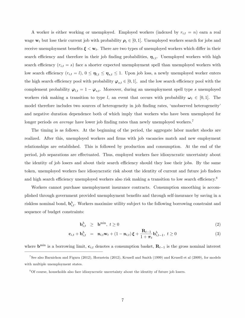
A worker is either working or unemployed. Employed workers (indexed by ri;t = n) earn a real

wage wt but lose their current job with probability �t 2 [0; 1]. Unemployed workers search for jobs and

receive unemployment bene�ts � < wt. There are two types of unemployed workers which di¤er in their

search e¢ ciency and therefore in their job �nding probabilities, �r;t. Unemployed workers with high

search e¢ ciency (ri;t = s) face a shorter expected unemployment spell than unemployed workers with

low search e¢ ciency (ri;t = l), 0 � �l;t � �s;t � 1. Upon job loss, a newly unemployed worker enters

the high search e¢ ciency pool with probability 's;t 2 [0; 1], and the low search e¢ ciency pool with the

complement probability 'l;t = 1 � 's;t. Moreover, during an unemployment spell type s unemployed

workers risk making a transition to type l, an event that occurs with probability !t 2 [0; 1]. The

model therefore includes two sources of heterogeneity in job �nding rates, �unobserved heterogeneity�

and negative duration dependence both of which imply that workers who have been unemployed for

longer periods on average have lower job �nding rates than newly unemployed workers.7

The timing is as follows. At the beginning of the period, the aggregate labor market shocks are

realized. After this, unemployed workers and �rms with job vacancies match and new employment

relationships are established. This is followed by production and consumption. At the end of the

period, job separations are e¤ectuated. Thus, employed workers face idiosyncratic uncertainty about

the identity of job losers and about their search e¢ ciency should they lose their jobs. By the same

token, unemployed workers face idiosyncratic risk about the identity of current and future job �nders

and high search e¢ ciency unemployed workers also risk making a transition to low search e¢ ciency.8

Workers cannot purchase unemployment insurance contracts. Consumption smoothing is accom-

plished through government provided unemployment bene�ts and through self-insurance by saving in a

riskless nominal bond, bhi;t. Workers maximize utility subject to the following borrowing constraint and

sequence of budget constraints:

bhi;t � bmin; t � 0 (2)

ci;t + bhi;t = ni;twt + (1� ni;t) � +

Rt�11 + �t

bhi;t�1; t � 0 (3)

where bmin is a borrowing limit, ci;t denotes a consumption basket, Rt�1 is the gross nominal interest

7See also Barnichon and Figura (2012), Hornstein (2012), Krusell and Smith (1999) and Krusell et al (2009), for models

with multiple unemployment states.

8Of course, households also face idiosyncratic uncertainty about the identity of future job losers.

7

rate, �t denotes the net in�ation rate in period t. ni;t indicates the household�s employment state:

ni;t =

8<: 1 if worker i is employed in period t

0 if worker i is unemployed in period t

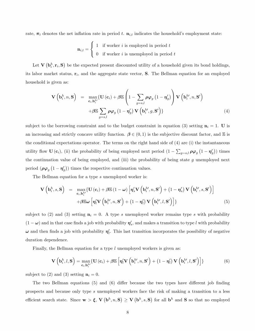
Let V�bhi ; ri;S

�be the expected present discounted utility of a household given its bond holdings,

its labor market status, ri, and the aggregate state vector, S. The Bellman equation for an employed

household is given as:

V�bhi ; n;S

�= max

ci;bh0i

fU (ci) + �E

0@1� Xg=s;l

�'g�1� �0g

�1AV �bh0i ; n;S0�+�E

Xg=s;l

�'g�1� �0g

�V�bh0i ; g;S

0�g (4)

subject to the borrowing constraint and to the budget constraint in equation (3) setting ni = 1. U is

an increasing and strictly concave utility function. � 2 (0; 1) is the subjective discount factor, and E is

the conditional expectations operator. The terms on the right hand side of (4) are (i) the instantaneous

utility �ow U (ci), (ii) the probability of being employed next period (1 �Pg=s;l �'g

�1� �0g

�) times

the continuation value of being employed, and (iii) the probability of being state g unemployed next

period (�'g�1� �0g

�) times the respective continuation values.

The Bellman equation for a type s unemployed worker is:

V�bhi ; s;S

�= max

ci;bh0i

fU (ci) + �E (1� !)h�0sV

�bh0i ; n;S

0�+�1� �0s

�V�bh0i ; s;S

0�i

+�E!h�0lV

�bh0i ; n;S

0�+�1� �0l

�V�bh0i ; l;S

0�ig (5)

subject to (2) and (3) setting ni = 0. A type s unemployed worker remains type s with probability

(1� !) and in that case �nds a job with probability �0s, and makes a transition to type l with probability

! and then �nds a job with probability �0l. This last transition incorporates the possibility of negative

duration dependence.

Finally, the Bellman equation for a type l unemployed workers is given as:

V�bhi ; l;S

�= maxci;bh0i

fU (ci) + �Eh�0lV

�bh0i ; n;S

0�+�1� �0l

�V�bh0i ; l;S

0�ig (6)

subject to (2) and (3) setting ni = 0.

The two Bellman equations (5) and (6) di¤er because the two types have di¤erent job �nding

prospects and because only type s unemployed workers face the risk of making a transition to a less

e¢ cient search state. Since w > �, V�bh; n;S

�� V

�bh; s;S

�for all bh and S so that no employed

8

household has an incentive to voluntarily leave their current job. Under the condition that �0s � �0l,

V�bh; s;S

�� V

�bh; l;S

�for all bh and S.

The consumption index ci is a basket of consumption goods varieties:

ci =

�Zj

�cji

�1�1= dj

�1=(1�1= )(7)

where cji is household i�s consumption of goods of variety j and > 1 is the elasticity of substitution

between consumption goods. Household i�s demand for variety j is given as:

cji =

�PjP

�� ci (8)

where Pj is the nominal price of variety j and P is a price index:

P =

�ZjP1� j dj

�1=(1� )(9)

Entrepreneurs. Consumption goods are produced by a continuum of measure < 1 of monop-

olistically competitive �rms indexed by j 2 (0;) which are owned by risk neutral entrepreneurs.

Entrepreneurs discount utility at the rate � and make decisions on the pricing of their goods, on va-

cancy postings, and on their consumption and savings policies. In return for managing (and owning)

the �rm, they are the sole claimants to its pro�ts. We assume that entrepreneurs can save but face

a no-borrowing constraint. This no-borrowing constraint implies that the entrepreneur �nances hiring

costs through retained earnings.9

Entrepreneurs make all their decisions simultaneously but we can separate them into the hiring and

pricing decisions made when acting as �rm owners and the consumption and savings choices made when

acting as households. Output is produced according to a linear technology:

yj;t = nj;t (10)

where nj;t denotes entrepreneur j�s input of labor purchased from the workers. Firms hire labor in a

frictional labor market. The law of motion for employment in �rm j is given as:

nj;t =�1� �t�1

�nj;t�1 + hj;t (11)

hj;t = tvj;t (12)

9 In the stationary equilibrium, � < 1= (R= ((1 + �))) so entrepreneurs will be borrowing constrained. This derives from

the assumption that households are risk averse while entrepreneurs are assumed risk neutral.

9

where hj;t denotes hires made by �rm j in period t, vj;t is vacancies posted, and t is the job �lling

probability. Firms are assumed to be su¢ ciently large that t can be interpreted as the fraction of

vacancies that leads to a hire.10 The cost of posting a vacancy is given by � > 0. Real marginal costs

are therefore:

mcj;t = wt +�

t� �Et

�(1� �t)

�

t+1

�(13)

Following Rotemberg (1982), �rms face quadratic costs of price adjustment. Given risk neutrality,

entrepreneurs set prices to maximize the present discounted value of pro�ts:

Et1Xs=0

�s

�Pj;t+sPt+s

�mcj;t+s�yj;t+s �

�

2

�Pj;t+s �Pj;t+s�1

Pj;t+s�1

�2yt

!(14)

subject to:

yj;t =

�Pj;tPt

�� yt (15)

Equation (15) is the demand for goods variety j. yt, can be interpreted as aggregate real income. In

equation (14) � � 0 indicates the severity of nominal rigidities in price setting with � = 0 corresponding

to �exible prices. The �rst-order condition for this problem is given as:�1� + mcj;t

PtPj;t

�yj;t = �

PtPj;t�1

�Pj;t �Pj;t�1Pj;t�1

�yt

���Et

" Pj;t+1P2j;t

!�Pj;t+1 �Pj;t

Pj;t

�Ptyt+1

#(16)

The entrepreneurs�consumption and savings decisions are the solutions to the following dynamic

programming problem:

W�bej ;nj ;S

�= maxdj ;be0j ;hj

�dj + �EW

�be0j ;n

0j ;S

0� (17)

subject to the employment transition equation and the budget and borrowing constraints:

dj + be0j +wnj + �

hj

=PjPnj �Te +

R�11 + �

bej (18)

be0j � 0 (19)

where dj denotes entrepreneur j�s consumption and be0j their bond purchases. Condition (19) imposes

the no-borrowing constraint on entrepreneurs. Te denotes a lump-sum tax imposed on employers to

cover the government provided unemployment bene�ts.

10This assumption - which is equivalent to assuming that is su¢ ciently smaller than 1, can be relaxed which would

produce ex-post heterogeneity across �rms.

10

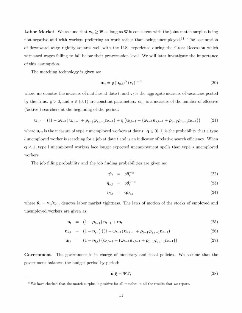
Labor Market. We assume that wt � w as long as w is consistent with the joint match surplus being

non-negative and with workers preferring to work rather than being unemployed.11 The assumption

of downward wage rigidity squares well with the U.S. experience during the Great Recession which

witnessed wages failing to fall below their pre-recession level. We will later investigate the importance

of this assumption.

The matching technology is given as:

mt = % (ua;t)� (vt)

1�� (20)

wheremt denotes the measure of matches at date t, and vt is the aggregate measure of vacancies posted

by the �rms. % > 0, and � 2 (0; 1) are constant parameters. ua;t is a measure of the number of e¤ective

(�active�) searchers at the beginning of the period:

ua;t =�(1� !t�1)us;t�1 + �t�1's;t�1nt�1

�+ q

�ul;t�1 +

�!t�1us;t�1 + �t�1'l;t�1nt�1

��(21)

where ur;t is the measure of type r unemployed workers at date t. q 2 (0; 1] is the probability that a type

l unemployed worker is searching for a job at date t and is an indicator of relative search e¢ ciency. When

q < 1, type l unemployed workers face longer expected unemployment spells than type s unemployed

workers.

The job �lling probability and the job �nding probabilities are given as:

t = %���t (22)

�s;t = %�1��t (23)

�l;t = q�s;t (24)

where �t = vt=ua;t denotes labor market tightness. The laws of motion of the stocks of employed and

unemployed workers are given as:

nt =�1� �t�1

�nt�1 +mt (25)

us;t =�1� �s;t

� �(1� !t�1)us;t�1 + �t�1's;t�1nt�1

�(26)

ul;t =�1� �l;t

� �ul;t�1 +

�!t�1us;t�1 + �t�1'l;t�1nt�1

��(27)

Government. The government is in charge of monetary and �scal policies. We assume that the

government balances the budget period-by-period:

ut� = Tet (28)

11We have checked that the match surplus is positive for all matches in all the results that we report.

11

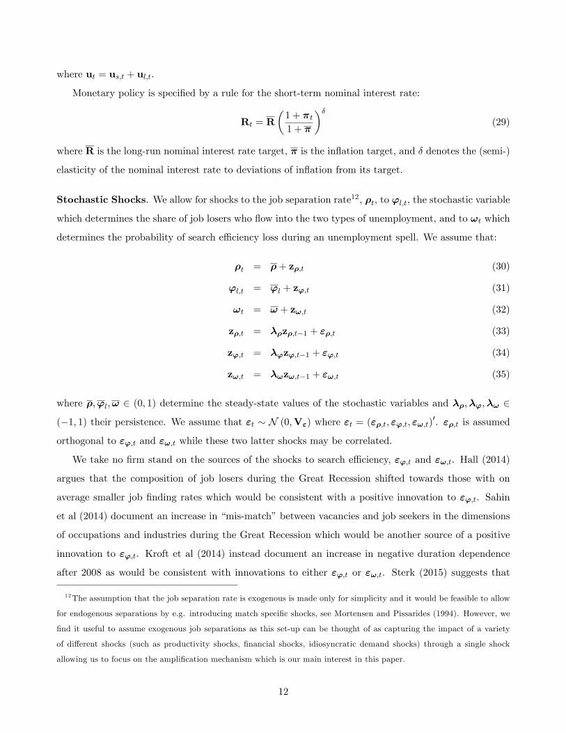
where ut = us;t + ul;t.

Monetary policy is speci�ed by a rule for the short-term nominal interest rate:

Rt = R

�1 + �t1 + �

��(29)

where R is the long-run nominal interest rate target, � is the in�ation target, and � denotes the (semi-)

elasticity of the nominal interest rate to deviations of in�ation from its target.

Stochastic Shocks. We allow for shocks to the job separation rate12, �t, to 'l;t, the stochastic variable

which determines the share of job losers who �ow into the two types of unemployment, and to !t which

determines the probability of search e¢ ciency loss during an unemployment spell. We assume that:

�t = �+ z�;t (30)

'l;t = 'l + z';t (31)

!t = ! + z!;t (32)

z�;t = ��z�;t�1 + "�;t (33)

z';t = �'z';t�1 + "';t (34)

z!;t = �!z!;t�1 + "!;t (35)

where �;'l;! 2 (0; 1) determine the steady-state values of the stochastic variables and ��;�';�! 2

(�1; 1) their persistence. We assume that "t � N (0;V") where "t = ("�;t; "';t; "!;t)0. "�;t is assumed

orthogonal to "';t and "!;t while these two latter shocks may be correlated.

We take no �rm stand on the sources of the shocks to search e¢ ciency, "';t and "!;t. Hall (2014)

argues that the composition of job losers during the Great Recession shifted towards those with on

average smaller job �nding rates which would be consistent with a positive innovation to "';t. Sahin

et al (2014) document an increase in �mis-match�between vacancies and job seekers in the dimensions

of occupations and industries during the Great Recession which would be another source of a positive

innovation to "';t. Kroft et al (2014) instead document an increase in negative duration dependence

after 2008 as would be consistent with innovations to either "';t or "!;t. Sterk (2015) suggests that

12The assumption that the job separation rate is exogenous is made only for simplicity and it would be feasible to allow

for endogenous separations by e.g. introducing match speci�c shocks, see Mortensen and Pissarides (1994). However, we

�nd it useful to assume exogenous job separations as this set-up can be thought of as capturing the impact of a variety

of di¤erent shocks (such as productivity shocks, �nancial shocks, idiosyncratic demand shocks) through a single shock

allowing us to focus on the ampli�cation mechanism which is our main interest in this paper.

12

falling house prices may have limited labor mobility during the Great Recession adding another source

of increase in 'l;t and !t.13 In short, there are multiple reasons for why heterogeneity in job �nding

prospects may have gone up during the Great Recession. Our approach is to capture these through 'l;t

and !t and analyze the extent to which their impact under some circumstances may be ampli�ed.

Equilibrium. We focus upon a recursive equilibrium in which workers act competitively taking all

prices for given while �rms act as monopolistic competitors setting the price of their own variety taking

all other prices for given. In equilibrium, �rms will be symmetric because of the absence of idiosyncratic

productivity shocks, state contingent pricing and because we assume that they are large enough that

job separation and vacancy �lling probabilities can be treated like fractions. We denote relative prices

by pj;t = Pj;t=Pt and note that symmetry implies that the equilibrium relative price equals 1 for all

goods. In the symmetric equilibrium, the optimal price setting condition therefore simpli�es to:

1� + mct = ��t (1 + �t)� ��Et��t+1 (1 + �t+1)

yt+1yt

�(36)

As is well-known, models with incomplete markets and aggregate shocks are cumbersome to solve

numerically. In this paper we follow Krusell, Mukoyama and Smith (2011) and impose that the bor-

rowing constraint bmin = 0. Under this assumption there is no aggregate savings vehicle available to

workers and, in equilibrium, since unemployed workers cannot issue debt, all workers consume their

income every period. Nonetheless, since employed workers face the risk of losing their job, they have an

incentive to save and will therefore be on their Euler equations. For the same reason, although workers

cannot save in equilibrium, the model still features a precautionary savings motive and this will impact

on equilibrium quantities through the real interest rate which will have to adjust to induce employed

workers not to save. The great advantage of imposing this borrowing constraint is that the aggregate

wealth distribution is degenerate which simpli�es the computational aspects of the model very consid-

erably. Moreover, Ravn and Sterk (2012) �nd that allowing for individual savings - and therefore for

a non-degenerate wealth distribution - has only limited impact on aggregate dynamics. The aggregate

state vector under the bmin = 0 borrowing constraint is given as St =�ul;t;us;t;�t;'s;t;!t

�which does

not involve the wealth distribution.

We let c�bh; r;S

�and bh0

�bh; r;S

�denote the decision rules that solve the workers� problems

(depending on their labor market status), and h (be;n;S) ; d (be;n;S) and be0 (be;n;S) the solutions

to the entrepreneurs�problem. We can now de�ne the equilibrium formally:

13The idea here is that geographical mobility (and therefore job �nding rates) may have declined for households which

experienced low or negative equity due to falling house prices.

13

De�nition 1 A recursive monopolistic competition equilibrium is de�ned as a state vector S, pricing

kernels (w (S) ;� (S)), decision rules�c�bh; r;S

�;bh0

�bh; r;S

��r=n;s;l

; (d (be;n;S) ;be0 (be;n;S) ;h (be;n;S))

and pj (be;n;S), value functions�Vn�bh;S

�;Vu;s

�bh;S

�;Vu;l

�bh;S

��andW (be;n;S), and govern-

ment policies (Te (S) ;R (S)) such that

(i) given the pricing kernel, the government policies, and the aggregate and individual states, the house-

hold decision rules solve the workers problems;

(ii) given the pricing kernel, government policies, and the aggregate state, the entrepreneur decision

rules solve the entrepreneurs�problem and pj (be;n;S) = 1 for all j and all (be;n;S);

(iii) asset, goods and labor markets clear:

0 =

Zibh0i

�bhi ; ri;S

�di+

Zjbe0j�bej ;nj ;S

�dj = 0

y � �v��2�2y =

Zichi

�bhi ; ri;S

�di+

Zjdj�bej ;nj ;S

�dj

y =

Zinhi diZ

jhj�bej ;nj ;S

�dj = % (ua;t)

� (vt)1��

nt =�1� �t�1

�nt�1 + % (ua;t)

� (vt)1��

ua;t =�(1� !t�1)us;t�1 + �t�1's;t�1nt�1

�+ q

�ul;t�1 +

�!t�1us;t�1 + �t�1'l;t�1nt�1

��us;t =

�1� �s;t

� �(1� !t�1)us;t�1 + �t�1's;t�1nt�1

�ul;t =

�1� �l;t

� �ul;t�1 +

�!t�1us;t�1 + �t�1'l;t�1nt�1

��(iv) the government budget constraint is satis�ed and the nominal interest is given by the policy rule in

equation (29) :

4 Quantitative Results

4.1 Calibration

We solve the model numerically using a standard perturbation approach (see the Appendix for details).

The calibration targets and parameter values are summarized in Tables 1 and 2.

One model period corresponds to a calendar month. The household utility function is assumed to

be given as:

U (ci;t) =c1��i;t � 11� � ; � � 0

14

� is the degree of relative risk aversion which matters for the household savings response to uncertainty.

We set � = 1:5 which is in the mid-range of empirical estimates of Attanasio and Weber (1995),

Eichenbaum, Hansen, and Singleton (1988), and many others who have examined either household data

or aggregate time series. We assume an annual real interest rate of 5 percent in the steady state and

set the subjective discount factor equal to 0:992 for both workers and entrepreneurs. This value is

low relative to standard representative agent models but because of idiosyncratic risk and incomplete

markets, agents have a strong incentive to engage in precautionary savings and a low real interest rate

is required to induce zero savings in equilibrium.

When calibrating the parameters pertaining to the labor market we must confront the issue that

the two types of unemployment are not directly observable.14 We address this issue by calibrating the

relevant parameters on the basis of information on labor market statistics that are informative about

the moments of interest. We target a steady-state unemployment rate of 5 percent. The parameters

(q;'s;!) and the steady-state job �nding probability for type s unemployed workers, �s, are calibrated

by targeting the following moments: First, according to CPS data for the post 1970 sample, on average

15 percent of job losers experience unemployment spells of 6 months or more. Secondly, the monthly

hazard rate for the newly unemployed is 43 percent, see Rothstein (2011). Third, we introduce in-

formation on duration dependence from Kroft et al�s (2013) estimate of the relationship between job

�nding probabilities and the length of an unemployment spell. These authors estimate the job �nding

probability of individuals out of work for d months at date t using a polynomial speci�cation for the

hazard. In particular, they assume that the job �nding rate depends on the length of the unemployment

spell and on labor market tightness as:

�t (�t; d) = A (d)m0�1��t

A (d) = (1� a1 � a2) + a1e�b1d + a2e�b2d

Using panel data from the CPS for the 2002-2007 sample (and controlling for demographic variables),

Kroft el al (2013) estimate ba1 = 0:314, ba2 = 0:393, bb1 = 1:085 and bb2 = 0:055. We target the impliedvalues of the relative hazard, A (d) =A (0), for integer values of d going up to 15 months.

We �nd that q = 0:468, 'l = 0:229; ! = 0:219 and �s = 0:586. Thus, 77 percent of job losers are

estimated to �ow into the high search e¢ ciency state upon job loss and thereafter face a moderate risk

of 22 percent per month of loss of search e¢ ciency during unemployment. Unemployed workers with

14Although type s unemployed workers have shorter expected unemployment spells than type l unemployed workers,

some of the type s unemployed will be out of work for extended periods due to bad luck.

15

high search e¢ ciency are more than twice as likely to �nd a job as low search e¢ ciency unemployed

workers implying that the unemployment state has a substantial impact on the expected unemployment

duration. In the steady-state, these parameter values imply that the average duration of the stock of

type s unemployed workers is 1.48 months, that the corresponding number for type l unemployed workers

is 4.10 months while the share of unemployed workers out of work for 6 months or more is 15.9 percent.

The calibration matches closely the hazard function estimated by Kroft et al�s (2013).15 Finally, to

match the 5 percent unemployment rate, we set the steady-state job separation rate (�) equal to 3.9

percent per month.

The bene�t level, �, is calibrated by targeting a decline in consumption of 11:7 percent upon unem-

ployment, a value which corresponds to Hurd and Rohwedder�s (2010) estimate of the average household

spending impact of a job loss.16 We assume that the matching function elasticity to unemployment, �,

is equal to 65 percent and we normalize % = 1. �, the vacancy cost parameter, is calibrated by targeting

an average hiring cost of 4:5 percent of the quarterly wage bill per worker. Given other parameters, this

implies that � = 0:19.

We set the average mark-up equal to 20 percent which implies that , the elasticity of substitution

between goods, is equal to 6. �, the parameter that determines the importance of price adjustment

costs, is calibrated to match a price adjustment frequency of 5 months. This value is conservative but

consistent with the estimates of Bils and Klenow (2004).17 This implies that � = 96:9. We assume

that the government�s in�ation target � = 0 so that it pursues price stability and we set � = 1:5, a

conventional value in the new Keynesian literature.

Finally, we estimate the parameters of the stochastic processes for �t, 'l;t and !t. The persistence

of �t and the variance of its innovation are estimated using JOLTS data on layo¤s and BLS estimates of

the employment rate for a sample ranging from 2003 to 2014.18 We �nd b�� = 0:91 and bv�=� = 0:0067.To estimate the persistence and volatility of 'l;t and !t we must again confront the issue that search

e¢ ciency is unobserved. However, we can use the model to �back out�processes for these two stochastic

15Figure A.1 in the Appendix illustrates the hazard function implied by our model evaluated in the steady-state together

with Kroft et al�s (2013) estimates.

16See http://www.nber.org/papers/w16407.pdf?new_window=1; Table 21. Browning and Crossley (2001) estimate a

similar average consumption loss due to unemployment shocks in Canadian household data.

17To be precise, we calibrate � by exploiting the equivalence between the log-linearized Phillips curve implied by our

model and the Phillips curve implied by the Calvo model.

18Our analysis focuses on the Great Recession and its aftermath and we choose the sample period accordingly.

16

shocks given the above estimate of the relative search e¢ ciency, q, the matching function parameters,

% and �, and data on the unemployment out�ow rate and labor market tightness. It follows from the

matching function that:

ua;t = ut�1

�e�t%

�1=�� vtut�1

�1�1=�(37)

where e�t is the average job �nding rate amongst the stock of unemployed. We further assume pro-portionality between 'l;t and !t which implies that the disturbances to these two �ows are perfectly

correlated and proportional, i.e. !'lz!;t = z';t. Under this assumption, we can use the estimates of ua;t

together with the transition equations (26)� (27) to derive estimates of 's;t and !t, see Appendix 2 for

details, from which we can estimate the persistence and variance of the two shocks. Using data from

JOLTS and the CPS (for the 2003-2014 sample) we �nd b�' = b�! = 0:99 and bv'='l = bv!=! = 0:072.194.2 Results

The Impact of Labor Market Shocks. We start by examining the impact of job separation shocks

and changes in the composition of unemployed workers. We compare the results of the benchmark

economy with two alternative economies. In the �rst of these we assume that prices are �exible (� = 0)

but retain the incomplete markets assumption. Comparing this economy with the benchmark model is

informative about the extent to which nominal rigidities matter for the transmission mechanism. In the

second alternative economy we assume that individuals can insure against idiosyncratic shocks within

large families (but retain the presence of nominal rigidities). In this alternative economy there is risk

sharing within the family so consumption is equalized across household members independently of their

labor market status which allows us to understand the extent to which idiosyncratic risk is important

for our results. In the risk sharing model the family maximizes utility subject to the single budget

constraint:

ct + bht = ntwt + (1� nt) � +

Rt�11 + �t

bht�1; t � 0

where nt is the fraction of employed household members in period t.

Figure 6 illustrates the responses of key aggregate variables to a one standard deviation increase

in the probability of job loss. Variations in the job termination rate have only moderate e¤ects on

19Since the frequency of the data is monthly, measured job openings and layo¤s are rather noisy. To avoid very erratic

shocks, we pre-smooth the data using a 6 month moving average �lter. The parameters of the shock processes are obtained

by regressing the shock variables on their values lagged with one year. We then compute the monthly persistence parameters

that are implied by the regressions.

17

equilibrium unemployment in standard matching models because rising unemployment implies declining

job �lling costs which triggers higher vacancy postings. In the benchmark model we instead �nd that

an increase in job separations produces a large increase in unemployment. Relative to the increase in

the job separation rate, unemployment rises a lot in the benchmark economy and in a very persistent

manner which also produces a surge in the share of longer term unemployed workers.20 Thus, not only

do workers see the job loss risk rising, but they also experience a worsening of job �nding prospects

during unemployment.

Figure 7 repeats the analysis for a joint one standard deviations increase in 's;t and in !t. This

combination of shocks generates a decrease in average search e¢ ciency because a larger proportion

of job losers �ow into type l unemployment and because a larger share of the existing high search

e¢ ciency unemployed workers su¤er a loss of search e¢ ciency. We �nd that these shocks also produce

a persistent increase in both the level of unemployment and in the share of longer term unemployed

workers. Similarly to the job separation shock, the decline in search e¢ ciency leads to a persistent

decline in vacancy postings and in the job �nding rate.

In order to understand better the results it is instructive to consider the Euler equation for employed

workers and the �rst order condition for price setting:

@U (cn) =@cn = �ER

1 + �0f�1� �

�'s�1� �0s

�+ (1�'s)

�1� �0l

���@U

�cn0�=@cn0

+�'s�1� �0s

�@U

�cu;s0

�=@cu;s0 + � (1�'s)

�1� �0l

�@U

�cu;l0

�=@cu;l0g (38)

1� + �w +

�

� �E (1� �x)

�

0

�= � (1 + �)� � ��E

�1 + �0

��0y0

y(39)

where cn denotes the consumption level of an employed worker, cu;s is consumption of a high search

e¢ ciency unemployed worker and cu;l is the consumption level of an unemployed worker with low search

e¢ ciency.

Employed workers are on their Euler equation because they have an incentive to save. Increased

risk of job loss (higher �) stimulate higher desired savings because it implies lower expected income and

because of increased idiosyncratic employment risk. Declining search e¢ ciency (lower 's) and worsening

job �nding prospects during unemployment (lower �0s or �

0l) imply longer expected unemployment spells

and therefore also trigger a decrease in expected household income and an increase in idiosyncratic

income risk both of which stimulate savings. Thus, when labor market conditions worsen, employed

workers�demand for consumption goods falls at the current real interest rate.

20The increase in job separations produces an initial short-lived drop in the fraction of long-term unemployed workers

because of the in�ow of newly unemployed workers.

18

Equation (39) is the optimal price setting condition in the symmetric equilibrium and it relates

in�ation to real marginal costs and to growth in aggregate output. Due to nominal rigidities (as

indexed by �), �rms �nd it optimal to phase in changes in the optimal price level gradually over time.

Adverse labor market conditions impact negatively on aggregate goods demand for the reasons just

discussed. In response to the drop in goods demand, it therefore follows that in�ation must fall which

needs to be accompanied by lower marginal costs. Since the real wage is assumed downward in�exible,

a fall in marginal costs has to come through a decline in the cost of hiring which requires the job �lling

rate, , to increase. Thus, vacancy postings have to fall which explains the persistent drop in the job

�nding rate. Finally, in response to the decline in in�ation, the central bank cuts nominal interest rates

su¢ ciently strongly to generate a drop in the real interest rate.

Thus, the model produces a simple and intuitive ampli�cation mechanism in which labor market

shocks trigger declining goods demand which are transmitted to the supply side and produce a fall in

labor demand. It is this transmission mechanism from the demand side to the supply side that produces

ampli�cation because fewer vacancies further depress labor market conditions and therefore stimulate

a further fall in goods demand.21

The transmission mechanism depends crucially on the combination of nominal rigidities in price

setting and on the lack of insurance against unemployment. To see this, Figures 5 and 6 also report the

impact of the labor market shocks for the two alternative economies described above. When prices are

�exible, job separation shocks have little impact on unemployment and lead only to a minor increase

in incidence of longer term unemployment. In this economy, price �exibility neutralizes the need for a

fall in marginal costs and �rms take advantage of low hiring costs (due to the increase in unemploy-

ment) to post more vacancies. The job �nding rate therefore falls only marginally which stops the

ampli�cation mechanism that operates in the benchmark economy. When the fraction of low search

e¢ ciency unemployed workers increases, it becomes more costly to �ll vacancies because the job �lling

rate declines. For that reason, this shock leads to a decline in vacancy postings which depresses the

job �nding rate and spurs precautionary savings. However, price �exibility once again eliminates the

need for a large decrease in vacancies and there is therefore no ampli�cation of the shock. Thus, even if

workers are exposed to idiosyncratic risk, price �exibility implies limited impact of deteriorating labor

market conditions.

21The no-borrowing constraint that we have imposed implies that the real interest rate does the full adjustment but it

should be understood that the transmission mechanism is one in which demand contracts in response to worsening labor

market conditions.

19

When workers can insure against idiosyncratic employment shocks through risk sharing within large

families changing labor market conditions no longer impact on idiosyncratic risk and savings are therefore

determined only by intertemporal considerations. An increase in the job separation rate impacts little

on the household because its e¤ect on expected family income is minor. For that reason, aggregate

demand is rather unresponsive to changes in the job separation rate in the economy with insurance.

The intertemporal savings motive is also small in the case of shocks to the share of low e¢ ciency

searchers and the presence of insurance within the family eliminates the precautionary savings e¤ect.

Thus, there is therefore little ampli�cation of labor market shocks when households can insure against

idiosyncratic risk.

In summary, the ampli�cation mechanism that arises in the benchmark economy derives from the

combination of nominal rigidities and the lack of insurance against idiosyncratic risk. Nominal rigidities

produces a channel through which variations in goods demand impact on job creation while the lack of

job insurance implies that changes in job prospects impact on goods demand.

The Great Recession. We now examine the extent to which the mechanisms of the model may be

important for understanding key features of the Great Recession. We derive estimates of the sequences

of the shocks, ("�;t; "';t; "!;t)2014:8t=2007:1 and we feed them into the model to produce counterfactual experi-

ments. "�;t is estimated by matching the observed U.S. time-series on the employment-to-unemployment

transition rate while "';t and "!;t are estimated using the same �model free�approach as above on the

basis of BLS and JOLTS data by matching the observed matching function residual. In order to avoid

having too erratic shocks, we smooth both data series with a 6 months moving average �lter. We then

feed the resulting shock processes into the model economy and simulate it in response to this particular

sequence of shocks.

The upper panels of Figure 8 illustrate the shocks that we estimate for the Great Recession. As

discussed in Section 2, the Great Recession witnessed a spur of job separations which started in early

2008, peaked in early 2009, and lasted only until the end of that year. The shock to search e¢ ciency

is estimated to be much more persistent. We �nd a steady rise in the share of new job losers that �ow

into low search e¢ ciency and in the share of high search e¢ ciency workers that experience a drop in

search e¢ ciency. The drop in the average search e¢ ciency starts in 2008 and continues throughout

2009/10 peaking in early 2011 and thereafter slowly diminishes. It is useful to compare this shock to

search heterogeneity with other measures. For that purpose we also illustrate "m;t:

"m;t = log

�1

%

�mt

ut�1

��1=�� vtut�1

�1�1=�!

20

"m;t is the matching function residual estimated by an econometrician who (wrongly) assumes homo-

geneous search e¢ ciency amongst the unemployed. The implied matching function residuals are very

similar to the estimates of Barlevy (2011) and correspond to a 40-45 percent adverse shock to the

matching function over the 2007-2011 period and a 20 percent recovery thereafter. We also illustrate

the fraction of newly unemployed workers who report to be �permanent� job losers. As argued by

Hall and Schulhofer-Wohl (2013), permanent job losers have lower job �nding rates than other types

of job losers and variations in this fraction therefore re�ect changes in average search e¢ ciency. This

fraction increases from 23 percent prior to the recession in 2007 to 45 percent by early 2010. Thereafter

it gradually declines towards its pre-recession level. It therefore mirrors quite precisely the matching

function residual implied by the shock to the heterogeneity in search e¢ ciency that we estimate.

Figure 9 illustrates the impact of the shocks on the level of unemployment, the number unemployed

workers out of work for 6 months or more (relative to the labor force), and on vacancies. In Section

2 we argued that the large drop in the job �nding rate and its very slow recovery thereafter are key

for understanding the severity of the Great Recession. A key focus of our analysis is therefore whether

the model can account for this response of the job �nding rate to the two labor market shocks just

discussed. The answer to this is a¢ rmative: Not only does the model reproduce the timing and the size

of the fall in the job �nding rate, but it is also consistent with the very persistent nature of the declining

job �nding prospects. Moreover, we �nd that the model accounts very closely for the adjustments in

unemployment and vacancies. As in the U.S. data, the level of unemployment surges in 2008 while the

number of vacancies implodes. Thereafter the increase in unemployment dissipates only very slowly over

time while vacancies recover slightly faster. The results demonstrate that the ampli�cation mechanism

discussed in the previous sections is quantitatively important.

Figure 9 also reports the share of longer term unemployed (the number of unemployed workers out

of employment for 6 months or more as a share of the total number of unemployed). This share soared

during the recession increasing from 15 percent prior to the recession to above 40 percent during 2010-

2012. The benchmark economy is consistent with the rise in the incidence of longer term unemployment

in the early part of the recession and with the very stubborn nature of the rise in this labor market

indicator. The model, however, is not fully able to account for the size of the rise in the incidence of

longer term unemployment since the peak in the share of longer term unemployed workers in the model

economy is just below 30 percent which is smaller and occurs earlier than in the U.S. data. Nevertheless,

the model does generate a signi�cant shift in the composition of the unemployed towards unemployment

states with longer duration.

21

Finally, the bottom left panel of Figure 9 displays the conditional standard deviation of income one

month ahead for currently employed workers, scaled by the current level of income.22 This is a measure

of the income uncertainty in the model which partly is endogenous as it depends on the job �nding

rate. We �nd that income uncertainty surges during 2008 and remains at an elevated level until 2013,

after which it decreases somewhat. Recall that there is little ampli�cation of the shocks in the �exible

price model. Therefore, by comparing with the corresponding measure in the economy without nominal

rigidities we can evaluate the endogenous component of this uncertainty measure. We �nd that income

uncertainty rises signi�cantly less in the �exible price economy than in the benchmark model especially

in the early part of the recession (the rise in income uncertainty by early 2009 is almost twice as large

in the benchmark economy as in the �exible price version of the model). It follows that the model

produces an important endogenous and countercyclical source of income uncertainty.

Combining the implications for the impact of the labor market shocks on unemployment and on

job vacancies produces the Beveridge curve illustrated in Figure 10. In the U.S. economy, there was

a rapid slide down the Beveridge curve in the early part of the recession followed by an outward shift

of this relationship and a gradual recovery in both indicators. Such counter-clockwise Beveridge curve

movements are not unusual during recessions but the current episode is more dramatic than what is

observed during most other recessions. We �nd that the model accounts very accurately for both the

movement down the Beveridge curve that occurred in 2008-2009 and the subsequent outward shift of

the Beveridge curve.

One might wonder about the extent to which job separation shocks and shocks to the search e¢ ciency

matter individually for these results. To understand this, Figures 8 and 9 also display the paths of the

relevant aggregates when we assume that the U.S. economy was hit only by job separation shocks. In

the absence of shocks to the �ows of workers to the two search e¢ ciency states, the model can account

for the initial rise in unemployment in late 2008 and for the initial drop in vacancies. However, the

shocks to search e¢ ciency are key for understanding both the size and the persistence of the rise in

unemployment and for the very long and deep decline in job vacancies. In addition when we exclude

the shocks to 't and to !t, the model produces only a very minor increase in the share of longer term

unemployed workers and little change in income uncertainty post 2010. This demonstrates that an

increase in heterogeneity amongst the unemployed is important for accounting for both the severity of

the Great Recession and for the surge in the incidence of longer term unemployment.

22To compute the conditional standard deviations we use a Gauss-Hermite approximation with 36 nodes. We do not

plot the uncertainty measure for the full insurance version of the model, as it is close to zero throughout the sample.

22

We can go further in understanding the mechanisms by examining the results when eliminating

frictions in goods or �nancial markets. When we assume that prices are �exible, the labor market

shocks leave vacancies almost una¤ected. For that reason, the worsening labor market conditions have

a much smaller impact on unemployment than in the data and lead to a very minor rise in the incidence

of longer term unemployment. Perhaps most strikingly, the �exible price model implies an extremely

counterfactual horizontal Beveridge curve. Interestingly, the model with insurance against idiosyncratic

shocks generates very similar results to the �exible price model. The labor market shocks have minor

impact on aggregate goods demand in this economy and for that reason �rms have little incentive to

post fewer vacancies in the wake of the worsening labor market conditions. The end result is a limited

increase in unemployment, a minor increase in the incidence of longer term unemployment, and a very

counterfactual horizontal Beveridge curve.

The key lesson we take away from this analysis is that the ampli�cation mechanism derives from the

combination of frictions in goods, labor and �nancial markets. Focusing on each of these frictions in

isolation may not be informative about the joint e¤ects and this potentially explains why past research

has concluded against the importance of labor market shocks for macroeconomic �uctuations. It is

important to stress that the shocks to search heterogeneity are not directly responsible for longer term

unemployment incidence. When we assume either risk sharing within large households or fully �exible

prices, these shocks are e¤ectively neutralized because they either have little impact on goods demand

(when assuming risk sharing) or are not transmitted to vacancy postings (when assuming �exible prices).

5 Extensions and Robustness Analysis

In this section we investigate four further issues. We �rst analyze further the sources of heterogeneity

in search e¢ ciency amongst the unemployed. Next, we examine the importance of the downward in�ex-

ible wage assumption and we look at how the monetary policy response matters for the ampli�cation

mechanism. Finally, we compare the results for the Great Recession with those for the early 1990�s

recession.

Search E¢ ciency Heterogeneity: Ampli�cation vs. Propagation. An important feature of

our model is the heterogeneity in search e¢ ciency amongst the unemployed. It is this aspect of the

model that allows us to address the substantial increase in the incidence of longer term unemployment

which has occurred during the Great Recession. Above we also argued that this feature is important

for accounting for the magnitude of the increase in unemployment and for its persistence.

23

Our analysis allows for heterogeneity in search activity to materialize either upon job loss or during

an unemployment spell (due to negative duration dependence). These two sources of heterogeneity

in search e¢ ciency play distinct roles. Heterogeneity in job search e¢ ciency upon job loss impacts

on employed workers�consumption and savings decisions directly, cf. the Euler equation (38). When

employed workers perceive higher risk of �owing directly into the low search e¢ ciency state should

they lose their job, they increase their desired precautionary savings. Increased risk of loss of search

e¢ ciency during an unemployment spell instead impacts on the average job �nding rate but does not

directly in�uence employed workers� savings choices and is therefore not directly important for the

ampli�cation mechanism. Negative duration dependence instead may act as a propagation mechanism

through which temporary increases in the number of job losers has persistent e¤ects because the pool

of newly unemployed workers risk experiencing a loss in their search e¢ ciency during an unemployment

spell.

We now wish to understand the extent to which the two �ows separately have been important for the

labor market dynamics during the Great Recession. Figure 11 repeats the Great Recession experiment

from the previous section under two alternative scenarios. In the �rst of these we assume that the

probability of search e¢ ciency loss during an unemployment spell, !t, remains constant during the Great

Recession and equal to its steady-state value of ! = 21:9 percent per month. This experiment informs

about the importance of changes in the two sources of heterogeneity for the labor market outcomes. In

the second experiment we set ! = 0 so that negative duration dependence is eliminated altogether so

that heterogeneity in search e¢ ciency derives solely from heterogeneous job �nding prospects upon job

loss.

We �nd that the path of the economy generated when assuming !t = ! is very similar to the one in

which we allow for both sources of changes in the extent of heterogeneity. This similarity relates both

to the share of longer term unemployed workers and to the level of unemployment. Thus, increased

heterogeneity in job �nding prospects upon unemployment is quantitatively much more important than

increased negative duration dependence. This result derives from the impact on precautionary savings

discussed above and it is consistent with the �ndings of Ahn and Hamilton (2014) who - studying

CPS data - �nd that recessions are times when there is an increased in�ow of workers with low job

�nding probabilities into unemployment. Our results go one step further and demonstrate that such

a compositional change is important for the severity of the Great Recession because of its impact on

aggregate demand.

We also �nd only a moderate e¤ect of eliminating negative duration dependence altogether (! = 0)

24

which indicates that the propagation mechanism that derives from workers experiencing a loss of search

e¢ ciency during an unemployment spell is rather limited. The reason for this is that our calibration

implies that type s workers �nd jobs quite fast (within 1.5 months on average in the steady-state) and

face a quite small risk of a loss of search e¢ ciency. Indeed, in the steady-state a type s unemployed

worker only faces a 13 percent risk of experiencing a transition to state l during an unemployment

spell. This risk is too small to matter much quantitatively. It follows that in the setting we examine,

heterogeneity in search e¢ ciency upon job loss is much more important for macroeconomic outcomes

than negative duration dependence.

The Role of Wage Flexibility. We have assumed that real wages are downward in�exible. This

assumption appears consistent with Figure 12 which shows that while the average real compensation

per hour worked in the Business Sector grew by approximately 25 percent from the mid-1990�s to the

beginning of 2007, real wages have remained unchanged since the onset of the Great Recession. We

will now ask two questions: First, to which extent do our results depend on this rigidity? Secondly, are

there circumstances under which a lack of a fall in real wages may arise as an equilibrium outcome?

In order to investigate these issues we assume that wages are determined according to a non-

cooperative Nash bargaining game between �rms and workers. We assume that in new matches, once

workers and �rms have been matched (but before a wage has been agreed upon), a worker enters the

two unemployment pools with probability 's;t and 1 � 'l;t, respectively, in exactly the same manner

as a worker who enters unemployment from an existing match.23 This assumption combined with the

borrowing constraint, makes the outcome under Nash bargaining particularly simple because the wage

o¤ered to a new worker is independent of their unemployment state.

We report results for a wide range of values of the workers�bargaining power which includes both

Hagedorn and Manovskii�s (2008) calibration of workers receiving 5 percent of the match surplus to

�traditional�values of this parameter of 50 percent. Figure 13 illustrates the impact of a job separation

shock on unemployment and on real wages. We report the maximum increase in unemployment relative

to the corresponding value in the benchmark model. Similarly, we show the maximum decline in the

real wage as a percentage of the steady-state real wage.24

We �nd that higher bargaining power on the part of workers implies higher wage �exibility in

23Alternatively, one can assume that workers retain their unemployment status but in this case the equilibrium would

entail one-period wage dispersion which seems unreasonable.

24We assume that workers enjoy leisure when unemployed and calibrate the utility value of leisure so that the steady-state

equilibrium real wage implies a 5 percent unemployment rate.

25

equilibrium and a signi�cantly smaller maximum response of unemployment. For example, when workers

and �rms have the same bargaining power, the maximum response of unemployment is less than 25

percent of the corresponding response in the benchmark economy. Low values of the workers�bargaining

power instead imply similar responses to labor market shocks to those we found when assuming in�exible

real wages.

To understand these results, consider the impact of an increase in the job separation rate on the joint

surplus. A higher job separation rate lowers the value of a �lled job because it increases the probability

that an existing match is terminated. It also lowers workers�outside option because of its impact on

the job �nding rate. Hence, the joint match surplus declines and this puts a downward pressure on real

wages which relieves the pressure on �rms to cut vacancy postings. The higher the workers�bargaining

power, the larger is the fall in real wages and the smaller is the decline in vacancy postings. Whether the

increase in job separations impact mostly on real wages or on vacancy postings matters for employed

workers�savings choices because the former of these have no impact on the precautionary savings motive

since it has no idiosyncratic risk component. For that reason, the ampli�cation mechanism is neutralized

when workers have a large bargaining power but not for low values of this parameter.

As we have noted above, real wages did not decline much, if at all, during the Great Recession.

The results presented here imply that this may either be consistent with workers have little bargaining

power or with real wages are downward in�exible. These two alternative scenarios have very similar

implications for equilibrium quantities and would therefore be di¢ cult to disentangle empirically.

The Role of Monetary Policy. It is standard intuition in the monetary economics literature that

aggressive responses of nominal interest rates to in�ation can neutralize the ine¢ ciencies that derive from

nominal rigidities while too weak responses to in�ation produce locally indeterminate equilibria. It is

unclear whether similar results should be expected to hold in the heterogenous agents model considered

in the current paper but the strength of the ampli�cation mechanism implies that the monetary policy

response may potentially be very important.

In order to investigate this issue, Figure 14 reports the impact of job separation rate shocks on

unemployment as a function of two key parameters, � and �.25 � determines the response of the

nominal interest rate to deviations of in�ation from its target while � determines the extent to which

workers respond to employment risk. We indicate by di¤erent colors the ampli�cation of the labor

market shocks in the benchmark economy by normalizing the maximum impact on unemployment of

25The results for mismatch shocks are nearly identical so we do not report them here.

26

the job separation shock with the equivalent response in a �exible price economy. A dark blue color

means no ampli�cation relative to the �exible price economy with lighter shades of blue and yellow

and orange colors indicating ever increasing degrees of ampli�cation. The white area corresponds to

combinations of � and � that are inconsistent with local determinacy of the equilibrium where in�ation

is on target.

We �nd that su¢ ciently aggressive monetary policy rules succeed in neutralizing the ampli�cation

mechanism while interest rate rules similar to those typically assumed in the New Keynesian literature

instead produce a large amount of ampli�cation. In our calibration (� = � = 1:5), both shocks are

signi�cantly ampli�ed but increasing � to around 2 neutralizes much of the ampli�cation relative to

the �exible price allocation. More aggressive of monetary policy responses provide stabilization by

moderating the agents�expectations regarding the impact of the shocks on equilibrium in�ation and

vacancy postings and thus impact directly on the mechanism through which labor market shocks are

ampli�ed.

Our results also show that higher degrees of risk aversion demand more aggressive policy rules in

order to provide stabilization and that, the higher is the degree of risk aversion, the more aggressive

has the interest rate rule to be in order to ensure local indeterminacy of the intended equilibrium.

These features derive from the impact of risk aversion on precautionary savings. When agents are

more risk averse, there is a stronger impact of labor market uncertainty on precautionary savings which

motivates the need for a more aggressive monetary policy stance in order to stabilize the economy.26 In

the indeterminacy region, equilibria can exist in which agents�expectations of worsening labor market

outcomes and low in�ation drives down aggregate demand thereby motivating �rms to hire less labor

and leading the economy to a high-unemployment-cum-low-in�ation self-ful�lling equilibria. Thus, the

design of the monetary reaction function is critical in the incomplete markets set-up analyzed in this

paper.

The Early 1990�s Recession. An important check on the extent to which the mechanisms that we

have emphasized are important can be conducted by applying the analysis to other recessions. For this

reason we now examine the early 1990�s recession. This recession witnessed a more shallow contraction

in output, an increase in the unemployment rate from 5 percent 1989 to above 7 percent in 1992

(a smaller increase than during the Great Recession) and a moderate increase (minor relative to the

26� also impacts on the determinacy region in standard New Keynesian models, see e.g. Gali (2008), but only because it

impacts on the response of consumption to real interest rates. In our model, a more important source of impact is through

precautionary savings.

27

Great Recession) in the share of longer term unemployment (see Figures 2 and 3). Similarly to the

Great Recession, the early 1990�s recession was associated with an increase in the job loss rate and a

persistent decline in the job �nding rate. Thus, there are similarities but also interesting di¤erences

between the Great Recession and the early 1990�s recession.

One issue that we must confront when applying the model to the early 1990�s recession is that

we do not have access to the same data as those that we used to estimate the shocks for the Great

Recession because we relied on JOLTS data for the layo¤ rate and for the number of job openings. We

follow Shimer (2005) and estimate the job termination rate on the basis of CPS measures of the number

of unemployed workers with duration below 5 months.27 We use Barnichon�s (2010) estimate of the

�composite help wanted index�to derive a measure of vacancies.28

Using these data we then repeat the exercise from Section 4.2 estimating the labor market shocks

and computing counterfactual paths of the key variables. Figure 15 illustrates the estimates of the job

separation shock and the search heterogeneity shocks for the early 1990�s recession. The increase in the

estimated job separation rate is marginally smaller than what was observed in the Great Recession but

very persistent. The heterogeneity shock instead is very small relative to the Great Recession and we

actually �nd a small reduction in the fraction of workers that �ow into the low search e¢ ciency state

from mid-1990 to mid-1991. This coincides with a small improvement in matching e¢ ciency in the early

part of the recession. From mid-1991 matching e¢ ciency worsens and we �nd a moderate increase in

the fraction of workers �owing into low search e¢ ciency.29

Figure 16 illustrates the counterfactual paths for unemployment, vacancies, the share of longer term

unemployed, the job �nding rate and the measure of income risk discussed earlier. The benchmark model

matches the data very well in terms of the paths of unemployment and vacancies. It also accounts for

the decline in the job �nding rate in the early part of the 1990�s recession but not quite for the extent

of the fall in the job �nding rate from 1992 to 1994. By contrast, when we assume either �exible prices

or lack of idiosyncratic income risk, the model implies little rise in unemployment and that vacancies

and the job �nding rate increase rather than fall. Thus, the ampli�cation mechanism that we have

discussed appears to be just as important for understanding the early 1990�s recession as for the Great

Recession. However, as anticipated, an important di¤erence between these two recessions is that the

27We correct for the redesign of the CPS in 1994 using the adjustment proposed in Elsby, Michaels and Solon (2009).

28We scale Barnichon�s composite index with the post 1970 index and we linearly detrend the data.

29We do not show the fraction of permanent job losers for this period, as this data series is only available from 1994

onwards.

28

search heterogeneity shock appears of little importance for the 1990�s recession since the countercyclical

paths of the economy are very similar with and without allowing for this shock.

Figure 17 illustrates the Beveridge curves. The data indicate that the US economy experienced a

slide down followed by an outward shift of the Beveridge curve during the 1990�s recession much like

what was witnessed during the Great Recession. However, both the movement along the Beveridge

curve and the outward shift were much smaller in the earlier of these two recessions. The benchmark

model again manages to account very well for these joint dynamics in unemployment and vacancies

with the di¤erence vis-à-vis the Great Recession being that the heterogeneity shock is not important

for the extent to which the model provides a good �t to the Beveridge curve dynamics.

We conclude from this that the central ampli�cation mechanism that we have stressed - the decline in

aggregate demand due to labor market risks and its transmission to the supply side - is equally important

for the early 1990�s recession as we claim it is for the Great Recession. The main contrast between these

two recessions was that the search heterogeneity shock was not important for the early 1990 recession.

For that reason, according to our results, this recession witnessed little rise in longer term unemployment

and a smaller rise in idiosyncratic income uncertainty which meant that this recession produced less

dramatic outcomes for the economy. Yet, in the absence of idiosyncratic income uncertainty or in the

presence of �exible prices, the early 1990�s recession would barely have increased unemployment.

6 Conclusions and Summary

We have shown how frictions in labor markets that interact with goods and �nancial markets frictions

can lead to a signi�cant ampli�cation of labor market shocks in a general equilibrium framework. At

the heart of our theory is the idea that labor market shocks that produce job uncertainty can reduce

aggregate goods demand because of precautionary savings. A calibrated version of the model can

account not only for the increase in unemployment observed in the U.S. during the Great Recession but

also for much of the movements in the Beveridge curve. It is the transmission of weak aggregate demand

to aggregate supply that produces these results because of an endogenous ampli�cation mechanism.

Our emphasis on job uncertainty deriving from idiosyncratic employment risk and uncertain out-

comes of labor market search o¤ers an additional route through which macroeconomic uncertainty can

impact on the economy. Much recent literature has focused upon uncertainty shocks deriving from

changes in the volatility of aggregate variables (such as TFP or policy related variables) and shown that

such uncertainty can be important for understanding aggregate �uctuations, see e.g. Bloom (2009). As

29

Carroll and Dunn (1997) we have instead focused on the idiosyncratic uncertainty implications of �rst

moment shocks to job loss and job �nding probabilities. We plan in future work to further examine the

importance of this channel using micro level data on consumption and labor supply.

Our theory has abstracted from aggregate savings and we imposed that workers cannot go into debt.

These assumptions are appealing from a computational perspective but it would be interesting to relax

them both so that one can also evaluate the impact on aggregate savings and investment. It would also

be interesting to investigate the impact of unemployment insurance policies. Unemployment insurance

duration is usually extended during U.S. recessions and the Great Recession is no exception to this.

Our exercise does take this into account because we focus entirely upon recessions and the calibration

of the level of bene�ts targets Hurd and Rohwedder�s (2010) estimates of the consumption loss due to

unemployment shocks during the Great Recession. Yet, it would be of interest to investigate further

how such cyclical variations in unemployment bene�ts impact on the aggregate outcomes. We plan to

pursue each of these issues in future work.

7 References

Ahn, Hie Joo, and James D. Hamilton. 2014. �Heterogeneity and Unemployment Dynamics.�

Mimeo, University of California at San Diego.

Attanasio, Orazio P., and Guglielmo Weber. 1995. �Is Consumption Growth Consistent with

Intertemporal Optimization? Evidence from the Consumer Expenditure Survey.� Journal of Political

Economy 103: 1121-57.

Barlevy, Gadi. 2011. �Evaluating the Role of Labor Market Mismatch in Rising Unemployment.�

Federal Reserve Bank of Chicago: Economic Perspectives 35: 82-97.

Barnichon, Regis. 2010. �Building a Composite Help-Wanted Index.�Economics Letters 109, 175-78.

Barnichon, Regis, and Andrew Figura. 2012. �Labor Market Heterogeneities, Matching E¢ ciency,

and the Cyclical Behavior of the Job Finding Rate.�Mimeo, Universitat Pompeu Fabra.

Basu, Susanto, and Brent Bundick. 2012. �Uncertainty Shocks in a Model of E¤ective Demand.�

Mimeo, Boston College.

Bils, Mark, and Peter J. Klenow. 2004. �Some Evidence on the Importance of Sticky Prices.�

Journal of Political Economy 112(5): 947-985.

Bloom, Nicholas. 2009. �The Impact of Uncertainty Shocks.�Econometrica 77(3): 623-85.

Browning, Martin, and Thomas F. Crossley. 2001. �Unemployment Insurance Bene�t Levels

30

and Consumption Changes.�Journal of Public Economics 80: 1-23.

Carroll, Christopher D. and Wendy Dunn. 1997. �Unemployment Expectations, Jumping (S,s)

Triggers, and Household Balance Sheets.�In: NBER Macroeconomics Annual 1997, edited by Benjamin

S. Bernanke and Julio Rotemberg (MIT Press: Cambridge, MA).

Carroll, Christopher D., Karen E. Dynan and Spencer D. Krane. 2004. �Unemployment

Risk and Precautionary Wealth: Evidence from Households�Balance Sheets.� Review of Economics

and Statistics 85(3).

Challe, Edouard, and Xavier Ragot. 2015. �Precautionary Saving over the Business Cycle.�

Forthcoming, Economic Journal.

Daly, Mary, Bart Hobijn, Aysegül Sahin and Rob Valletta. 2011. �A Rising Natural Rate of

Unemployment: Transitory or Permanent?�WP 2011-05, Federal Reserve Bank of San Francisco.

Eichenbaum, Martin, Lars P. Hansen and Kenneth Singleton. 1988. �A Time Series Analysis

of the Representative Consumer Models of Consumption and Leisure under Uncertainty.�Quarterly

Journal of Economics 103(1): 51-78.

Elsby, Michael, Bart Hobijn, and Aysegül Sahin. 2010. �The Labor Market in the Great

Recession.�Brookings Papers on Economic Activity : 1-48.

Elsby, Michael, Ryan Michaels, and Gary Solon. 2009. �The Ins and Outs of Cyclical Unem-

ployment.�American Economic Journal: Macroeconomics 1(1): 84-110.

Gornemann, Nils, Keith Kuester, and Makoto Nakajima. 2012. �Monetary Policy with Het-

erogeneous Agents.�Mimeo, Federal Reserve Bank of Philadelphia.

Guerrieri, Veronica, and Guido Lorenzoni. 2015. �Credit Crisis, Precautionary Savings and the

Liquidity Trap.�Mimeo, University of Chicago Booth School of Business.

Hagedorn, Marcus, and Iourii Manovskii. 2008. �The Cyclical Behavior of Equilibrium Unem-

ployment and Vacancies Revisited.�American Economic Review 98(4): 1692-1706.

Hall, Robert E. 2014. �Quantifying the Lasting Harm to the U.S. Economy from the Financial Crisis.�

Forthcoming, NBER Macroannual 2014.

Hall, Robert E. and Sam Schulhofer-Wohl. 2013. �Measuring Matching E¢ ciency with Hetero-

geneous Jobseekers. Manuscript, Stanford University.

Hornstein, Andreas. 2011. �Accounting for Unemployment: The Long and Short of It.�Manuscript,

Federal Reserve Bank of Richmond.

Hurd, Michael D. and Susann Rohwedder. 2011. �The E¤ects of the Financial Crisis on Actual

and Anticipated Consumption.�Working Paper no. 255, University of Michigan, Michigan Retirement

31

Research Center.

Katz, Lawrence F. 2010. �Long-Term Unemployment in the Great Recession.�Testimony for Joint

Economic Committee. U.S. Congress: Hearing on �Long-Term Unemployment: Causes, Consequences

and Solutions�, Washington D.C.: April 29.

Krusell, Per, Toshihiko Mukoyama, Aysegül Sahin and Anthony A. Smith Jr. 2009. �Re-

visiting the Welfare E¤ects of Eliminating Business Cycles.� Review of Economic Dynamics 12(3):

393-402.

Krusell, Per, Toshihiko Mukoyama, and Aysegül Sahin. 2010. �Labor-market matching with

precautionary savings and aggregate �uctuations.�Review of Economic Studies 77 (4): 1477-1507.

Krusell, Per, Toshihiko Mukoyama and Anthony A. Smith Jr. 2011. �Asset Prices in a Huggett

Economy.�Journal of Economic Theory 146(3): 812-44.

Krusell, Per and Anthony A. Smith Jr. 1999. �On the Welfare E¤ects of Eliminating Business

Cycles.�Review of Economic Dynamics 2(1): 245-272.

Leduc, Sylvain, and Zheng Liu. 2013. �Uncertainty Shocks are Aggregate Demand Shocks.�Federal

Reserve Bank of San Francisco working paper no. 2012-10.

McKay, Alisdair, and Ricardo Reis. 2014. �The Role of Automatic Stabilizers in the U.S. Business

Cycle.�NBER working paper no.19000.

Mortensen, Dale T. and Christopher A. Pissarides. 1994. �Job Creation and Job Destruction

in the Theory of Unemployment.�Review of Economic Studies 61(3), 397-415.

Ravn, Morten O. and Vincent Sterk. 2012. �Job Uncertainty and Deep Recessions.� Mimeo,

University College London.

Rendahl, Pontus. 2012. �Fiscal Policy in an Unemployment Crisis.�Mimeo, Cambridge University.

Rotemberg, Julio J. 1982. �Sticky Prices in the United States.�Journal of Political Economy 90(6):

1187-1211.

Rothstein, Jesse. 2011. �Unemployment Insurance and Job Search in the Great Recession.�Brookings

Papers on Economic Activity 43(2): 143-213.

Sahin, Aysegül, Joseph Song, Giorgio Topa and Gianluca Violante. 2012. �Mismatch Unem-

ployment.�Manuscript, New York University.

Schaal, Edouard. 2012. �Uncertainty, Productivity and Unemployment in the Great Recession.�

Mimeo.

Shimer, Robert. 2005. �The Cyclical Behaviour of Equilibrium Unemployment and Vacancies.�

American Economic Review 95(1), 25-49.

32

Sterk, Vincent. 2015. �Home Equity, Mobility, and Macroeconomic Fluctuations.�Journal of Mon-

etary Economics 74, 16-32.

Wiczer, David. 2013. �Long Term Unemployment: Attached and Mismatched?�Mimeo, University

of Minnesota.

33

7.1 Appendix 1: Solving and simulating the model

From the no-borrowing constraint it follows that, in equilibrium, the individual workers�consumption

levels are given as cul = cus = � and cn = w. We can then reduce the model down to a core dynamic

subsystem of only three equations: the household�s Euler equation for bonds, Equation (38), the �rms�

pricing condition, Equation (39) and the monetary policy rule, Equation (29), which can be written as:

w�� = �ER

1 + �0f�1� �

�'s�1� �0s

�+ (1�'s)

�1� �0l

���w��

+�'s�1� �0s

���� + � (1�'s)

�1� �0l

����g

1� + �w + %

11����

�1��s � �E (1� �) %

11����

0 �1��s

�= � (1 + �)� + ��E

�1 + �0

��0y0

y

Rt = R

�1 + �t1 + �

��We use this dynamic system of three equations, together with the exogenous shock processes, to solve

for the equilibrium laws of motions of �s;t, Rt and �t using a standard perturbation method.30 We can

then simulate these variables for a given time path of the exogenous shocks.

Simulations of the remaining variables are obtained using the original nonlinear equations. Given

a simulation for �s;t, Rt and �t and the shocks, we can use Equations (22)-(23) directly to obtain

simulations for �t and t. Next we jointly use Equations (20)-(21) and (25)-27) to recursively �nd

the simulation paths for mt, ua;t, nt, us;t and ul;t; given initial conditions for us;t and ul;t. To �nd

the time path for vacancies and the unemployment rate, we use the condition that vt = �t=ua;t and

ut = 1 � nt. The average job �nding rate is computed as mtut�1+�t�1nt�1

. Finally, a simulation for

the share of unemployed for 6 months or less is obtained by recursively keeping track of the mass of

unemployed in each of the two states by duration, ranging from 1 to 6 months.

7.2 Appendix 2: Retrieving shocks from the data

We retrieve the search e¢ ciency shocks z';t and z!;t from the data using an iterative accounting

procedure based on only the model�s labor market transition equations and the matching function.

Importantly, the values of the shocks are found independently of the model solution for �s;t, rt and �t:

Thus, key features of the model�s ampli�cation mechanism such as the degrees of price stickiness, risk

aversion and market incompleteness have no impact on the values of the shocks we retrieve from the

data.

30This is done after substituting out �l;t = q�s;t in the Euler equation and exploiting that the termy0

ydrops out under

a �rst-order approximation of the model around a steady- state with � = 0.

34

Our procedure is based on three data series: (i) the civilian unemployment rate from the BLS, (ii)

the layo¤ rate from JOLTS, and (iii) the number of job openings from JOLTS. The �rst step is to

retrieve a time series for the number of active searchers, ua;t, from the data. To this end, we re-write

the matching function, Equation (20), as:

mt = %

�ua;tut�1

��(ut�1)

� (vt)1�� :

and note that�ua;tut�1

��is the time-varying residual of an aggregate matching function that abstracts

from heterogeneity. Thus, a by-product we obtain a time series for the aggregate matching function

residual and the shocks we back out map exactly into this residual.

To proceed, we rearrange the above equation to obtain an expression for ua;t:

ua;t = ut�1

�e�t%

�1=�� vtut�1

�1�1=�where e�t � mt

ut�1=

1�ut�(1��t�1)(1�ut�1)ut�1

. Given time series for ut; �t and vt we can evaluate the entire

right-hand side of the above equation. For consistency with the model�s steady state, we take the log

of both sides of the equation and subtract the mean, which gives:

bua;t = but�1 + 1=� be�t + (1� 1=�) (bvt � but�1)where a hat denotes a log deviation from the mean.31 We then construct a time series for the fraction

of active searchers as ua;t = eua+bua;t ; where ua is the steady-state level of active searchers in the model.Given ua;t we can compute the job �nding rate among searchers in each period:

�s;t =mt

ua;t

= e�tut�1ua;t

which also gives a time series for �l;t = q�s;t. Next, we back out the shocks using the following iterative

procedure:

1. Start at t = 1, initializing us;0 and ul;0 are at their steady-state levels.

2. Using our proportionality assumption !t = (!='l)'l;t and 's;t�1 = 1�'l;t�1; re-write equation

(21) to obtain an expression for 'l;t�1 :

'l;t�1 =ua;t � us;t�1 � �x;t�1nt�1 � qul;t�1

� (!=�l)us;t�1 � �x;t�1nt�1 + q (!=�l)us;t�1 + q�x;t�1nt�1

31The scaling�s parameter % drops out of the equation. The matching parameter � is set to 0:65, to be consistent with

our model calibration.

35

Evaluate the right-hand side to obtain 'l;t�1, and compute the implied values of !t�1 and 's;t�1:

3. Use Equations (27) and (27) to compute us;t and ul;t.

4. Set t = t+ 1 and go back to step 2 until t = T:

5. Once the time series for 'l;t and !t have been obtained, back out z';t and z!;t from Equations

(33) and (34).

Our procedure uses data over the period January 2003 until August 2014.

7.3 Appendix 3: The Nash bargaining problem

Under the assumptions discussed in the main text, the Nash Bargaining solution satis�es:

��

= (1� �) [V (b; e;S)�'lV (b; l;S)� (1�'l)V (b; s;S)] =U

0(w);

where � is the bargaining power of the worker and � is the surplus of a match to an entrepreneur, which

is equal to the (expected) resource cost of hiring a new worker. The term between square brackets on the

right-hand side is the surplus of a match to a household, which equals the di¤erence between the value

obtained in an employment relationship, V (b; e;S) ; minus the expected value outside the relationship,

'lV (b; l;S) + (1�'l)V (b; s;S). The multiplicative term U0(w) on the right-hand side converts the

utility surplus of the employed worker into units of resources using her marginal utility.

To solve the model, we add the Nash bargaining condition to the system of equations, as well as

the worker value expressions, Equations (4)-(6), setting c = w for the employed worker�s value and

c = � for the unemployed workers of each type. The latter requirement follows from the borrowing

constraint b � 0 which implies that �as in the baseline model�workers consume their current-period

income streams.

Relative to the baseline model, the system to be solved thus contains four additional equations (value

functions for the three worker types and the Nash Bargaining condition) and four additional variables

(worker values for the three types and the real wage). We solve this model using �rst-order perturbation

on the entire system of model equations.

7.4 Appendix 4. The Hazard Function

We calibrate� = (';!;q;�s) by targeting a 15 percent steady-state share of workers out of employment

with a duration of unemployment of 6 months or more, a steady-state monthly job �nding probability

36

of 43 percent, and the hazard function implied by Kroft et al�s (2013) estimates. These authors estimate

the hiring probability of individuals out of work for d months at date t using a polynomial speci�cation

for the hazard:

�t (�t; d) = A (d)m0�1��t

A (d) = (1� a1 � a2) + a1e�b1d + a2e�b2d

Using panel data from the CPS for the 2002-2007 sample their estimates are ba1 = 0:314, ba2 = 0:393,bb1 = 1:085 and bb2 = 0:055. Third, we introduce information on duration dependence from Kroft et

al�s (2013) estimate of the relationship between hiring probabilities and the length of an unemployment

spell. These authors estimate the hiring probability of individuals out of work for d months at date t

using a polynomial speci�cation for the hazard. In particular, they assume that the job �nding rate

depends on the length of the unemployment spell and on labor market tightness as:

�t (�t; d) = A (d)m0�1��t

A (d) = (1� a1 � a2) + a1e�b1d + a2e�b2d

Using panel data from the CPS for the 2002-2007 sample for d going up to 15 months (and controlling for

demographic variables), Kroft et al (2013) estimate ba1 = 0:314, ba2 = 0:393, bb1 = 1:085 and bb2 = 0:055.We calibrate � by minimizing the quadratic form:

W =�� (�)� �target

�0 �� (�)� �target

�where � (�) are the model implied moments and �target are the targets just listed. The minimization

problem delivers the estimates � = (0:229;0:219;0:468;0:586). The �gure below illustrates the

implied hazard function along with Kroft et al�s (2013) estimates.

37

0 5 10 150.4

0.5

0.6

0.7

0.8

0.9

1

unemployment duration (d) in months

outfl

ow h

azar

d re

lativ

e to

 d=0

Kroft et al. (2013)model

Figure A.1: Hazard function

38

7.5 Tables and Figures

Table 1: Targets and Parameter Values

Targets

0.05 unemployment rate (u)

0.586 job �nding rate among searchers (�s)

0.045 s.s. hiring cost as a fraction of the quarterly wage ( � 4w )

0.15 fraction of long-term unemployed (> 6 months)

0.117 consumption loss upon unemployment ( �w )

0 net in�ation rate (�)

0.05 annual net interest rate (R12�1)

5 average price duration (in months) in equivalent version with Calvo pricing

Parameter Values

� 96.9 price adjustment cost parameter

6 elast. subst. goods varieties

� 0.992 discount factor

� 1.5 coe¢ cient of relative risk aversion

� 1.5 interest rate rule parameter on in�ation

� 0.039 steady state job termination rate

�� 0.91 persistence parameter termination rate

100��=� 0.667 std. dev. � shock as a percentage of �

'l 0.229 steady state fraction of job losers into s-pool

! 0.219 steady state fraction from s-pool to l-pool

�' 0.99 persistence of shocks to fraction of job losers into l-pool

100�'='l 7.20 std. dev. 'l shock as a percentage of 'l

�! 0.99 persistence of shocks to fraction from s-pool to l-pool

100�!=! 7.20 std. dev. ! shock as a percentage of !

� 0.19 matching e¢ ciency parameter

q 0.468 probability of search for unemployed in l-pool

w 0.830 real wage

� 0.65 matching function elasticity

� 0.733 unemployment bene�t

R� 1 0.004 steady-state net nominal interest rate

39

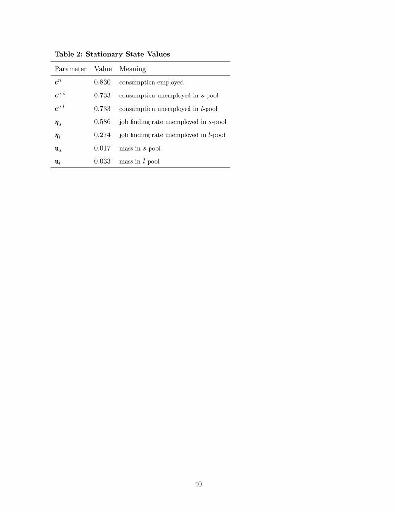
Table 2: Stationary State Values

Parameter Value Meaning

cn 0.830 consumption employed

cu;s 0.733 consumption unemployed in s-pool

cu;l 0.733 consumption unemployed in l-pool

�s 0.586 job �nding rate unemployed in s-pool

�l 0.274 job �nding rate unemployed in l-pool

us 0.017 mass in s-pool

ul 0.033 mass in l-pool

40

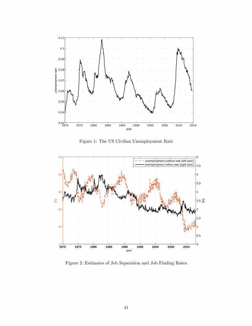
1970 1975 1980 1985 1990 1995 2000 2005 2010 20150.03

0.04

0.05

0.06

0.07

0.08

0.09

0.1

0.11

unem

ploy

men

t rat

e

year

Figure 1: The US Civilian Unemployment Rate

1970 1975 1980 1985 1990 1995 2000 2005 201010

20

30

40

50

60

(%)

year1970 1975 1980 1985 1990 1995 2000 2005 2010

0

0.5

1

1.5

2

2.5

3

3.5

4

4.5

5

(%)

unemployment outflow rate (left axis)unemployment inflow rate (right axis)

Figure 2: Estimates of Job Separation and Job Finding Rates

41

1970 1975 1980 1985 1990 1995 2000 2005 2010 20150

0.05

0.1

0.15

0.2

0.25

0.3

0.35

0.4

0.45

0.5

year

shar

e un

empl

oyed

 >6m

Figure 3: Share of unemployed workers who have been out of work for 6 months or more

1990 1995 2000 2005 2010 20155

10

15

20

25

30

35

40

45

50

year

average duration (weeks)inverse of  job f inding rate (weeks)recursive estimate duration (weeks)f raction of  unemployed > 6m (percent)

Figure 4: Average Unemployment Duration and Estimates from Job Finding Rates

42

4 6 8 10 12 14 1620

30

40

50

60

70

80

90

100

110

120

unemployed workers (millions)

vaca

ncy 

inde

x (ja

n 20

07 =

 100

)

2001­20062007­2014

Figure 5: The Beveridge Curve

43

0 10 20 30 400.0389

0.039

0.0391

0.0392

0.0393job termination rate

0 10 20 30 400.0495

0.05

0.0505

0.051unemployment rate

0 10 20 30 400.158

0.159

0.16

0.161

0.162

0.163

0.164fraction of unemployed with duration > 6m

0 10 20 30 403.17

3.18

3.19

3.2

3.21

3.22average unemployment duration (months)

0 10 20 30 400.465

0.47

0.475

0.48average job finding rate

sticky pricesflexible pricesfull insurance

0 10 20 30 40­0.04

­0.03

­0.02

­0.01

0

0.01vacancies

0 10 20 30 400.0486

0.0501

0.0511real interest rate (annualized)

benc

hmar

k / f

lexi

ble 

pric

es

0 10 20 30 400.0986

0.1001

0.1011

full 

insu

ranc

e

0 10 20 30 40­15

­10

­5

0

5x 10 ­4 inflation rate (annualized)

Figure 6: The Impact of Job Separation Shocks

44

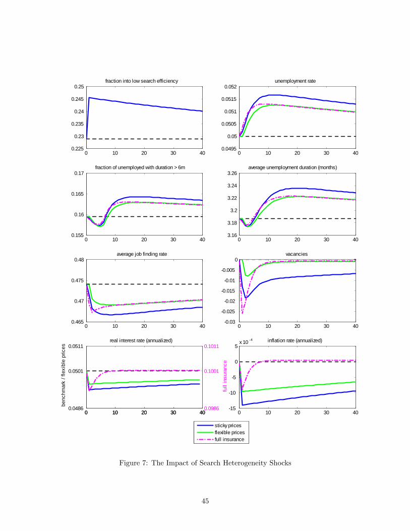
0 10 20 30 400.225

0.23

0.235

0.24

0.245

0.25fraction into low search efficiency

0 10 20 30 400.0495

0.05

0.0505

0.051

0.0515

0.052unemployment rate

0 10 20 30 400.155

0.16

0.165

0.17fraction of unemployed with duration > 6m

0 10 20 30 403.16

3.18

3.2

3.22

3.24

3.26average unemployment duration (months)

0 10 20 30 400.465

0.47

0.475

0.48average job finding rate

sticky pricesflexible pricesfull insurance

0 10 20 30 40­0.03

­0.025

­0.02

­0.015

­0.01

­0.005

0vacancies

0 10 20 30 400.0486

0.0501

0.0511real interest rate (annualized)

benc

hmar

k / f

lexi

ble 

pric

es

0 10 20 30 400.0986

0.1001

0.1011

full 

insu

ranc

e

0 10 20 30 40­15

­10

­5

0

5x 10 ­4 inflation rate (annualized)

Figure 7: The Impact of Search Heterogeneity Shocks

45

2007 2008 2009 2010 2011 2012 2013 20140.038

0.039

0.04

0.041

0.042

0.043

0.044termination rate

2007 2008 2009 2010 2011 2012 2013 20140.2

0.3

0.4

0.5

0.6

0.7

0.8

0.9fraction into low search efficiency

2007 2008 2009 2010 2011 2012 2013 2014­0.4

­0.3

­0.2

­0.1

0

0.1matching function residual

log 

poin

ts

2007 2008 2009 2010 2011 2012 2013 20140.2

0.25

0.3

0.35

0.4

0.45

0.5unemployment: fraction of permanent job losers

Figure 8: The Great Recession: Shocks

46

2007 2008 2009 2010 2011 2012 2013 20140

0.1

0.2

0.3

0.4

0.5share of unemployed >6m

2007 2008 2009 2010 2011 2012 2013 20140.25

0.3

0.35

0.4

0.45

0.5average job finding rate

2007 2008 2009 2010 2011 2012 2013 20140.04

0.05

0.06

0.07

0.08

0.09

0.1

0.11unemployment rate

2007 2008 2009 2010 2011 2012 2013 201420

40

60

80

100

120vacancy index (s.s.=100)

sticky pricesflexible pricesfull insuranceonly termination rate shocksdata

2007 2008 2009 2010 2011 2012 2013 20141.5

1.6

1.7

1.8

1.9

2income uncertainty employed

% o

f cur

rent

 inco

me

Figure 9: The Great Recession

47

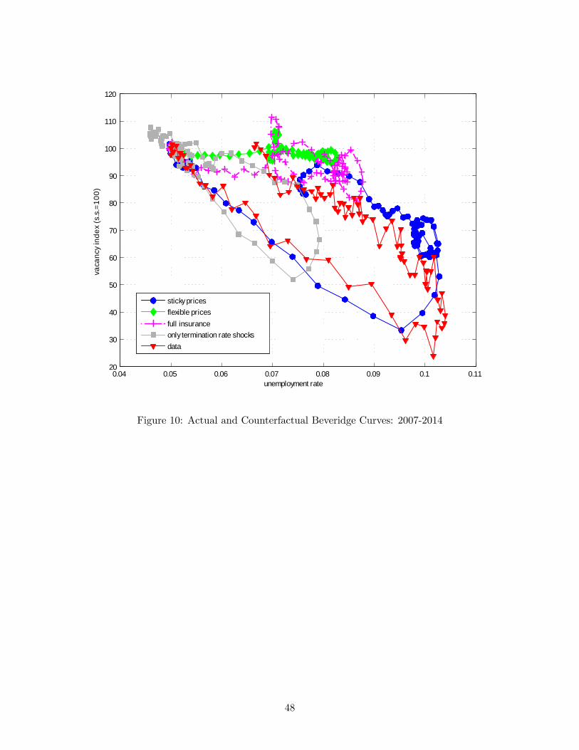
0.04 0.05 0.06 0.07 0.08 0.09 0.1 0.1120

30

40

50

60

70

80

90

100

110

120

unemployment rate

vaca

ncy 

inde

x (s

.s.=

100)

sticky pricesflexible pricesfull insuranceonly termination rate shocksdata

Figure 10: Actual and Counterfactual Beveridge Curves: 2007-2014

48

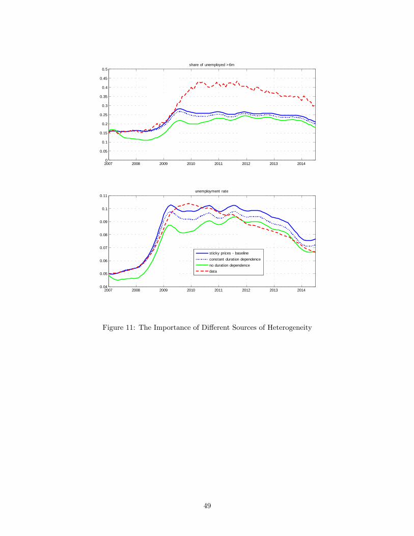
2007 2008 2009 2010 2011 2012 2013 20140

0.05

0.1

0.15

0.2

0.25

0.3

0.35

0.4

0.45

0.5share of unemployed >6m

2007 2008 2009 2010 2011 2012 2013 20140.04

0.05

0.06

0.07

0.08

0.09

0.1

0.11unemployment rate

sticky prices ­ baselineconstant duration dependenceno duration dependencedata

Figure 11: The Importance of Di¤erent Sources of Heterogeneity

49

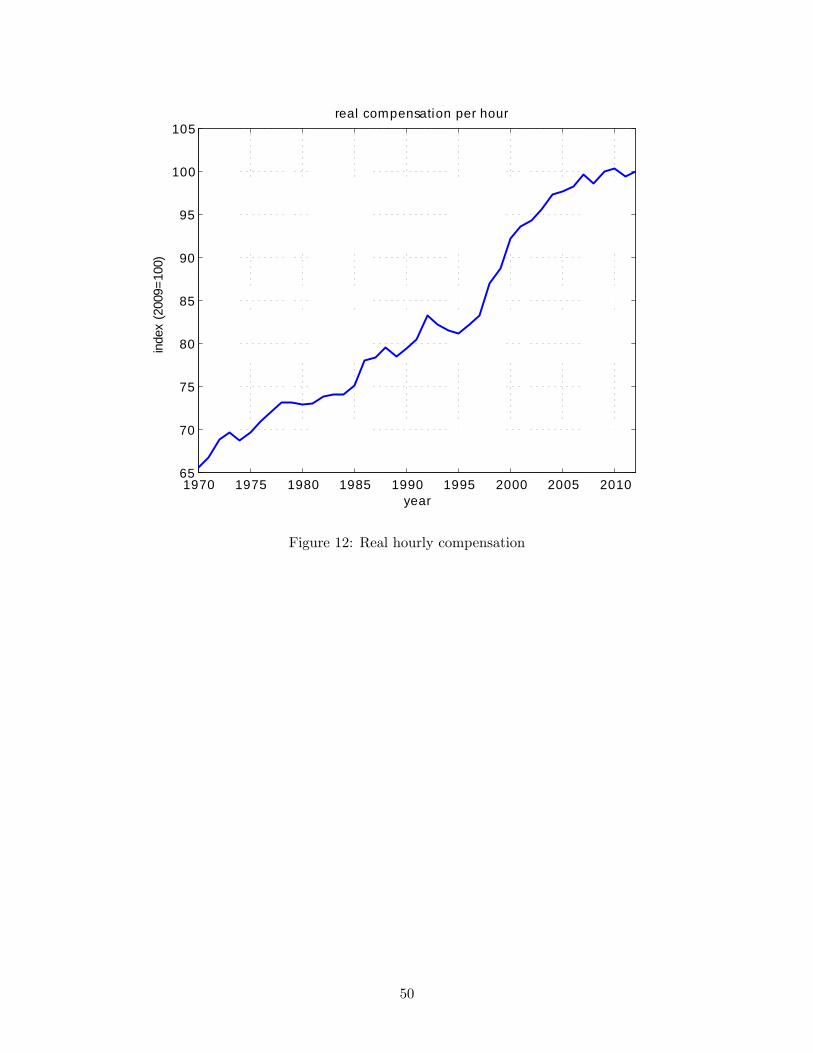
1970 1975 1980 1985 1990 1995 2000 2005 201065

70

75

80

85

90

95

100

105real  compensation per hour

inde

x (2

009=

100)

year

Figure 12: Real hourly compensation

50

0 0.05 0.1 0.15 0.2 0.25 0.3 0.35 0.4 0.45 0.50.02

0.03

0.04

0.05

0.06

0.07

0.08

0.09

0.1

bargaining power worker

max

imum

 resp

onse

 une

mpl

oym

ent r

ate 

(%­p

oint

s)

0 0.05 0.1 0.15 0.2 0.25 0.3 0.35 0.4 0.45 0.5­0.02

­0.015

­0.01

­0.005

0

0.005

0.01

bargaining power worker

max

imum

 resp

onse

 real

 wag

e (%

)

Figure 13: The Importance of Increased Duration Dependence

51

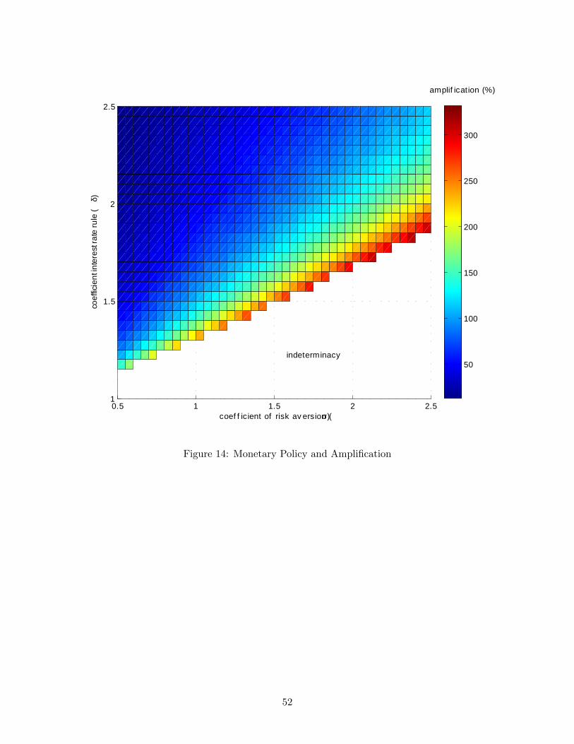
0.5 1 1.5 2 2.51

1.5

2

2.5

coef f icient of  risk av ersion (σ)

coef

ficie

nt in

tere

st ra

te ru

le (

δ)

50

100

150

200

250

300

amplif ication (%)

indeterminacy

Figure 14: Monetary Policy and Ampli�cation

52

1990 1991 1992 1993 19940.0385

0.039

0.0395

0.04

0.0405

0.041

0.0415

0.042

0.0425

0.043termination rate

1990 1991 1992 1993 19940.1

0.15

0.2

0.25

0.3

0.35fraction into low search efficiency

1990 1991 1992 1993 1994­0.1

­0.08

­0.06

­0.04

­0.02

0

0.02matching function residual

log 

poin

ts

Figure 15: Early 1990�s Recession: Shocks

53

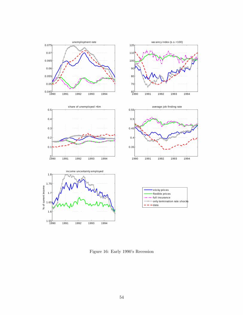
1990 1991 1992 1993 19940

0.1

0.2

0.3

0.4

0.5share of unemployed >6m

1990 1991 1992 1993 1994

0.35

0.4

0.45

0.5

0.55average job finding rate

1990 1991 1992 1993 19940.045

0.05

0.055

0.06

0.065

0.07

0.075unemployment rate

1990 1991 1992 1993 199460

70

80

90

100

110

120vacancy index (s .s .=100)

sticky pricesflexible pricesfull  insuranceonly termination rate shocksdata

1990 1991 1992 1993 19941.55

1.6

1.65

1.7

1.75

1.8income uncertainty employed

% o

f cur

rent

 inco

me

Figure 16: Early 1990�s Recession

54

0.04 0.05 0.06 0.07 0.08 0.09 0.1 0.1120

30

40

50

60

70

80

90

100

110

120

unemploy ment rate

vaca

ncy 

inde

x (s

.s.=

100)

sticky  pricesf lexible pricesf ull insuranceonly  termination rate shocksdata

Figure 17: Actual and Counterfactual Beveridge Curves: 1990-1995

55