joel voigt - 24227730 - finalyearreport-mec4401

FINGERING INSTABILITIES AT

THE EDGE OF ADVANCING

BACTERIA BY: JOEL VOIGT

PROJECT UNDERTAKEN TOGETHER WITH JEDIDIAH KENWRIGHT

SUPERVISED BY: DR PRABHAKAR RANGANATHAN

Final Year Project 2015

Final Report

2

SUMMARY The computational modelling of a bacterial growth known as Pseudomonas Aeruginosa is explored

based on the variation of model parameters in this report. Since there is no known techniques that

can effectively mitigate and inhibit the growth of this bacteria, a computational simulation based on

elastic forces of a single cell was created to successfully reproduce this growth. This report includes

work from previous student including the mathematical modelling and solution techniques to run the

given equations based on discretization, crank-nicolson and gauss-jordan techniques. The procedures

looking into node redistribution and intersection stitching are also explained. Improvements to

computational modelling in regards to void removal, cell-alignment term alteration and contour

extraction are introduced and thoroughly explained. These new additions allow for a more accurate

simulation. Lastly the impact of parameters such as the friction coefficient, mass growth rate, alpha

cell and the bending rigidity and surface tension are explained. The initially parabolic term in the cell

orientation equation yields a higher degree of ‘fingering’ when it is of a linear order. For values above

101 for alpha cell and mass growth rate, a significant rate of growth and contours is observed. It was

also seen that altering the friction coefficient had a minimal impact compared to the other variables,

however it was still a useful measure in controlling the rate of colony growth. Switching off the

contractive forces allowed for an uninhibited growth which could be linked to actual bacterial growth

in controlled testing circumstances. More research and testing is required for any advancements in

this field, however a better understanding and improvement of the current simulation was achieved.


Final Report

3

TABLE OF CONTENTS Summary ................................................................................................................................................. 2

Table of Contents ............................................................................................................................ 3

1. Introduction ............................................................................................................................ 5

2. Analytical Methodology .......................................................................................................... 7

2.1 Mathematical Representation of Bacterial Growth ........................................................ 7

2.2 Solution Method ............................................................................................................. 7

2.2.1 Discretization of equations ..................................................................................... 7

2.2.2 Crank-Nicolson method for solving governing equations ....................................... 7

2.2.3 Gauss-Jordan solver of matrix equations ................................................................ 8

3. Existing Model ......................................................................................................................... 8

3.1 Curvature-Dependence ................................................................................................... 8

3.2 Exponential Mass Growth ............................................................................................... 9

3.3 Cell Self-Propulsion ......................................................................................................... 9

3.4 Computational Procedures ........................................................................................... 10

3.4.1 Node redistribution ............................................................................................... 10

3.4.2 Intersection stitching ............................................................................................ 10

4. Updated Model ..................................................................................................................... 11

4.1 Void Removal ................................................................................................................ 11

4.2 Cell Alignment Term Alteration .................................................................................... 12

4.3 Contour Extraction ........................................................................................................ 13

4.4 Computational Anomalies............................................................................................. 14

4.5 Limitations ..................................................................................................................... 15

5. Effect of Model Parameters .................................................................................................. 15

5.1 Influence of Initial Cell Orientation (𝛷) ......................................................................... 16

5.2 Impact of Bending Rigidity and Surface Tension on Stability (к and ϒ) ........................ 19

5.3 Effect of Alignment Forcing Constant (φcell) .................................................................. 21

5.4 Effect of Friction Coefficient (𝜂) ................................................................................... 24


Final Report

4

5.5 Effect of Specific Mass Growth Rate (𝜇) ....................................................................... 26

6. Future Work .......................................................................................................................... 28

6.1 Revised Model ............................................................................................................... 28

6.2 Further Suggestions ...................................................................................................... 29

7. Conclusions ........................................................................................................................... 29

8. Acknowledgements ............................................................................................................... 30

9. References ............................................................................................................................ 30

10. Appendices ........................................................................................................................ 31


Final Report

5

1. INTRODUCTION

Due to advancements made within the medical industry over the past decade, research and application into the modelling of cell migration has been an important focus and challenge. One of the current challenges is the colonization of specific bacterial cells between implanted devices and host tissue, leading to the spread of infection (Mark et. Al 2010). Understanding the growth patterns of various pathogenic bacteria holds the key to developing medicine that is able to firstly mitigate the spread of said bacteria and furthermore inhibit such growth. To reach a sufficient understanding of the growth patterns of bacteria, it was proposed that an accurate computational simulation was to be created. Our project will be exploring and expanding on a current simulation of a bacteria known as Pseudomonas aeruginosa based on computational values and models from previous research students (Sweeney and Zadnik 2014). Pseudomonas aeruginosa is a motility-mediated bacterium that can be commonly found in medical equipment such as catheters (Pseudomonas aeruginosa 2015). Pseudomonas aeruginosa has been found to be highly resistant and able to genetically mutate in order to adapt to antibiotics as it contains more than 50 resistant genes (Pseudomonas aeruginosa 2015). Colonization occurs through burrowing and expanding biofilms of Pseudomonas aeruginosa, causing intricate networks of furrows. These networks begin as ‘fingers’ protruding from the original colony as the cells advance in the direction of the leading edges of these fingers. These fingers are seen to join with each other creating these intricate networks of bacteria until the colony has reached its maximum growth capacity. The behaviour observed in the growth of Pseudomonas aeruginosa colonies can be deemed highly ordered and coordinated (Mark et. Al 2010). The specific mechanisms that are responsible for coordinating this complex behaviour remain unknown; however it is expected to contain a mixture of physical, chemical and biological factors. A purely physical model produces a very similar structure under certain conditions and therefore applying a completely fluid based model will yield similar ‘cell-like’ formations. This model includes surface instabilities and these finger-like patterns that have been observed (Mark et. AL 2010) based on two fluids confined in a thin layer, if the driving fluid has a lower viscosity compared with the secondary fluid (Saffman & Taylor 1958).

Figure 1. A magnification of a colony of Pseudomonas aeruginosa (Pseudomonas aeruginosa 2015)

Based on modelling detailed in a previous paper (Sweeney and Zadnik 2014), a set of equations have been created to accurately represent the growth of Pseudomonas aeruginosa in regards to elastic forces. However due to the lack of knowledge surrounding the physical parameters of Pseudomonas aeruginosa, such as surface tension and bending rigidity random values have been assigned to


Final Report

6

produce a similar growth pattern to the real life colonization. Past work from these students has focused on a curvature dependent force model and the addition of the increasing mass of cells and stitching which allowed ‘finger-like’ structures to join and form intricate networks that continue to grow. A cell–self propulsion model was also generated as a more accurate representation of the ‘finger-like’ rafts seen in the growth of Pseudomonas aeruginosa. The passive relaxation state was also manipulated to accurately model the growth rate. There are a number of limitations that are highlighted in the previous paper (Sweeney and Zadnik 2014):

1. The previous model suggests all cell motion is based only on movement of the outer contours however individual cell motion and movement is not accounted for

2. Experimental values have been arbitrarily selected for the elastic forces and other components since the actual values are unknown

3. The effect of interior contours on the interface has not been explored or modelled

The main focus for our project coincided with the second limitation of the previous paper. With the goal of more accurately modelling a colony of Pseudomonas Aeruginosa based on computational simulations of a viscous fluid encapsulated within a thin film, the cell orientation, bending rigidity, surface tension, alignment forcing constant, friction coefficient and specific mass growth rate were varied. Simulations were then obtained, as well as, graphical representations of the interfaces area, density, number of contours and velocity over a given number of time steps. Initially the proposed aims of the project were:

1. To understand the current model and its accompanying code to allow for alteration and

improvement.

2. To manipulate various parameters in the current model to accurately create a stable and

long-lived lattice structure.

3. To examine the effect of model parameters on the shapes and sizes of lattice voids as well as

on the growth rate of the interface.

4. Suggest methods that can be applied for mitigating the spread of infection.

Aims one, two and three were successfully completed however more research and understanding is

required to achieve the fourth aim.

This report outlines in the following order – the analytical model used to simulate Pseudomonas

Aeruginosa based on a force balance of a single cell. The previous model will be explored and the

additions of stitching and node redistribution will also be explained. Following this, the updated model

will be introduced with the inclusion of void removal, contour extraction, anomalies and cell alignment

term alteration. The effects of the various model parameter previously mentioned will then be

investigated. Lastly an outline of suggestions for future work and a revised model will be provided for

any further improvements that will lead to the fourth aim being reached.


Final Report

7

2. ANALYTICAL METHODOLOGY

2.1 Mathematical Representation of Bacterial Growth

From the previous paper it was assumed the motion of the colony was based on a simple force balance

of a single cell in a viscous fluid. The projected forces include elastic restoring forces which consist of

bending rigidity and surface tension. These cause the computational colony to contract. Furthermore

a forcing function was added to overcome the elastic contractive forces and achieve a given growth

rate based on the motility of the cells. Finally the viscous friction was included since the simulation is

based on a fluid between two surfaces.

(1)

𝑟 is the position vector of any point of the interface of the contour, whilst ɳ is the coefficient of

viscous friction (Sweeney and Zadnik 2014). к and ϒ are the bending modulus and surface tension,

respectively. �⃗�𝑐𝑒𝑙𝑙is based on the cell orientation at various curvatures.

(2)

2.2 Solution Method

2.2.1 Discretization of equations

The initial equation modelling bacterial growth (Eq. 2) was challenging and time-consuming to solve

analytically, therefore it was appropriate to implement a discretization that was compatible with the

Crank-Nicholson method (Sweeney and Zadnik 2014). This allowed the governing equation to be

solved based on the second order of a Taylor series expansion using the forward-time center-space

method. The second order expansion allowed for a combination of accuracy and reasonable

computational time.

The forward-time center-space method requires each term that consists of the forward time-step

(t+Δt) to be stored on one side of the equation and each term that involves the current time (t) to be

on the other side. This ensures each future time-step is solved in terms of the current time-step and

is constantly updating itself based on its previous shape and form.

2.2.2 Crank-Nicolson method for solving governing equations

After discretization of the governing equation the Crank-Nicolson method (3) for solving PDE’s was

used based on its implicit nature and less stringent stability requirements (Sweeney and Zadnik 2014).

Implicit methods require much less computational time to achieve a given accuracy even with larger

time steps making it a desirable technique to use. The techniques hinges on compiling unsolved

equations at a given time step into a matrix which is then solved simultaneously.


Final Report

8

(3)

The Crank-Nicolson method is based on the trapezoidal rule and is a combination of the forward Euler

method and backward Euler method.

2.2.3 Gauss-Jordan solver of matrix equations

To solve for the matrix equations from the Crank-Nicholson PDE the direct Gauss-Jordan matrix

scheme was selected (Zadnik and Sweeney 2014). This was a desirable technique compared to others

because the correct solution is obtained without limiting the time step size.

(4)

Gauss-Jordan elimination method is an algorithm used for solving matrices of linear equations. For a

given unsolved matrix as seen in figure 4, the gauss-jordan method uses row operations to simplify

the given matrix into row echelon form. Consequentially the equations can then easily be solved and

applied to a simulation.

3. EXISTING MODEL

3.1 Curvature-Dependence

Initially the forcing term in Eq.2 was set to a constant value however this didn’t replicate the growth

of a colony. A curvature-dependent model was then added based on the assumption that the forcing

function is zero for any positive integer curvatures and linearly increasing as the negative curvatures

increased linearly (Sweeney and Zadnik 2014). This more accurately replicated a colony of bacteria.

From Eq.7, H is the equivalent curvature between nodes on the interface and from (6), α is the force

gradient.

(6)

(7)


Final Report

9

3.2 Exponential Mass Growth

To further improve upon the curvature dependent model, since actual colony growth isn’t as

symmetrical in nature, was to incorporate a term that takes into account the growing mass resulting

from cell reproduction (Sweeney and Zadnik 2014).

Due to Pseudomonas Aeruginosa’s exponential reproductive nature Eq.8 was assumed based on the

initial mass and specific growth rate. Eq.9 calculates the density based on the mass over the

instantaneous area. α from Eq.6 is updated to 𝐹0𝑒𝑝(𝑡)−𝑝0

𝑝0 , accounting for the exponential rate of

change of the density and hence, mass growth rate.

(8)

(9)

(10)

3.3 Cell Self-Propulsion

Previous models still lacked growth patterns exhibited by Pseudomonas Aeruginosa, most notably the

finger-like rafts that extend outwards from the colonies interface. Therefore to replicate this motion

computationally, it was assumed that the ‘fingering’ rafts were resultant of forces applied by individual

cells in the direction of their individual axes (Sweeney and Zadnik 2014).

An additional term 𝜑 takes into account the propelling force based on cell orientation. 𝛼𝑐𝑒𝑙𝑙 is the

coefficient that sets the strength of the orientation dependent force. Coupled with the curvature

dependence, the orientation force completes the new model seen in Eq.11.

(11)

(12)

Assuming that in an actual colony that cells can be knocked out of alignment and the occurrence of

cell jostling is present, an equation that takes these factors into account and that determines how

the cell orientation changes with time at the interface was constructed (Eq.13). The equation models

the relaxation rate of the model based on the given curvature at any point on the interface.


Final Report

10

(13)

Eq.13 can be solved by an O.D.E and is added explicitly into the matrix equations to be solved by the

gauss-jordan elimination technique since it could not easily be included in the Crank-Nicolson

scheme due to elementary requirements. This model best represented the ‘finger-like’ rafts seen

propelling outward from the interface.

3.4 Computational Procedures

3.4.1 Node redistribution

To perform a Crank-Nicholson discretization from section 2.2.2 all contour segments must be of equal

length. This required a linear interpolation between nodes at the beginning of each time step to

ensure this constraint was met. It was also necessary to run this node redistribution seven times to

ensure each segment was updated based on the current contour at the given time step. This

redistribution is run at the beginning of each time step and consists of the following:

1. The total length of the contour is calculated based on the addition of the linear segments

between nodes

2. The equal segments are calculated simply by dividing the contour length from step 1 by the

desired number of nodes

3. Finally, each node is then placed in the appropriate segments by interpolating linearly

between nodes

3.4.2 Intersection stitching

To overcome self-intersection (as seen in figure 2) at the interface which is uncharacteristic of a

bacterial growth, a stitching code was proposed and implemented. The stitching had to detect when

the interface had self-intersected and then redistribute nodes to form an updated, continuous

interface and then allow the remaining nodes to make up a void within or outside of the boundary.

The model would then continue to propagate as normal according to the model equations. This

stitching technique allowed the model to further replicate a growth of Pseudomonas Aeruginosa and

increase the models accuracy.

Implemented to detect when the interface has self-intersected and to redistribute the nodes to form

an updated interface and the remaining nodes to make up a void within or outside the boundary

depending on the type of intersection. The remaining nodes at the continuous interface then continue

to propagate according to the model equations. The effect of this code can be seen in figure 3.


Final Report

11

(Figure 2 – Pre-stitching computational simulation)

(Figure 3 – Post-stitching computational simulation)

4. UPDATED MODEL

4.1 Void Removal

In the previous model each void would reduce down to a small speck but never disappear which can

be observed in figure 4. This is obviously uncharacteristic of a colony of Pseudomonas Aeruginosa, so

a new code was written to more accurately simulate a colony growth and delete each speck. The new

void removal code goes through every contour and calculates their length. Contours that are below a

set minimum length and/or have less than five nodes (Crank-Nicholson requirement) are removed.

This prevents oscillation of contours of about zero size. In graphical terms the sharp drops in area and

the oscillations in the velocity are results of the voids being removed based on the rate the given

contour is changing (rapidly or slowly). The effect of the new model can be seen in figure 5.


Final Report

12

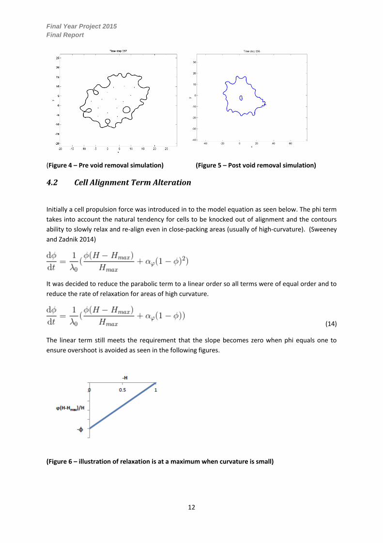
(Figure 4 – Pre void removal simulation) (Figure 5 – Post void removal simulation)

4.2 Cell Alignment Term Alteration

Initially a cell propulsion force was introduced in to the model equation as seen below. The phi term

takes into account the natural tendency for cells to be knocked out of alignment and the contours

ability to slowly relax and re-align even in close-packing areas (usually of high-curvature). (Sweeney

and Zadnik 2014)

It was decided to reduce the parabolic term to a linear order so all terms were of equal order and to

reduce the rate of relaxation for areas of high curvature.

(14)

The linear term still meets the requirement that the slope becomes zero when phi equals one to

ensure overshoot is avoided as seen in the following figures.

(Figure 6 – illustration of relaxation is at a maximum when curvature is small)


Final Report

13

(Figure 7 – illustration that relaxation rate reduces to zero as cells are close to aligned)

The difference in growth patterns can be observed in section 5.1.

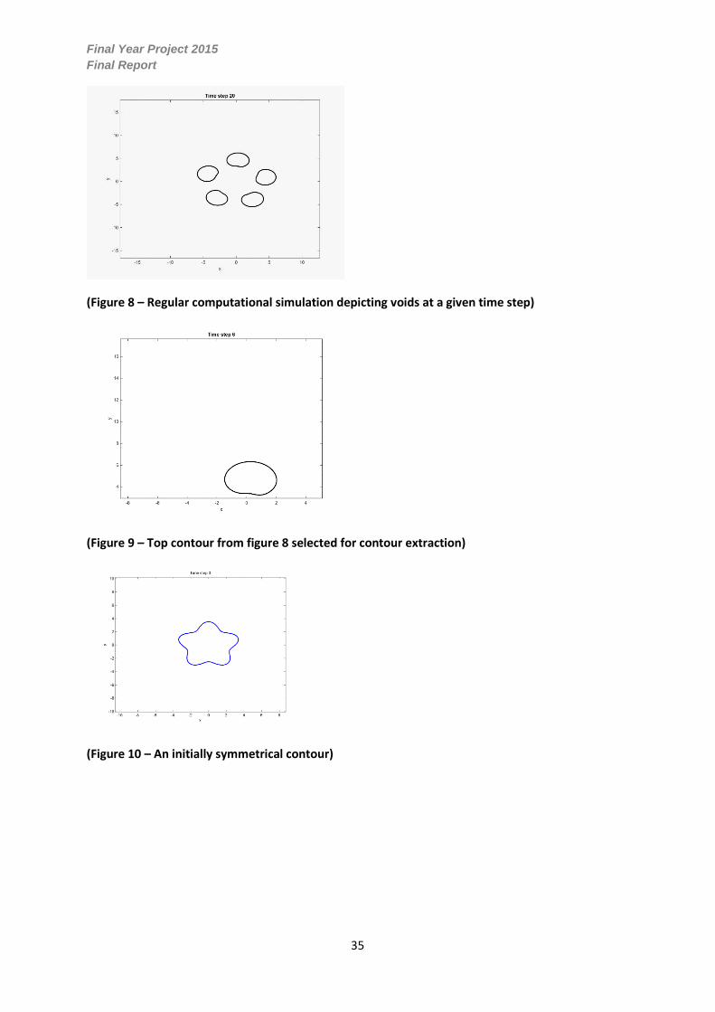
4.3 Contour Extraction

The initial code allowed the user to run a simulation of the model and investigate the growth of each

contour relative to one another. It was proposed that a code that allowed the user to isolate a single

contour after running a complete simulation was to be added.

The contour extractor extracts the co-ordinates as well as the phi values of the specified contour (user

selected) and runs a simulation of the selected contour over the given time steps. The following figures

show a complete simulation and then a simulation of the top contour running the contour extraction

code.

(Figure 8 – Regular computational simulation depicting voids at a given time step)


Final Report

14

(Figure 9 – Top contour from figure 8 selected for contour extraction)

This method is useful for observing the growth and movement of a given contour without the

distraction of the other contours. It is also a much quicker method to run that an entire simulation

and can provide some more obvious insight into a contours growth.

4.4 Computational Anomalies

Despite using symmetrical initial conditions, the model becomes asymmetrical over time as seen in

the following figures. This is resultant of computational variability and instability during the numerical

simulations. The computational anomalies are an accurate representation of an actual colony of

pseudomonas aeruginosa since stable conditions can only exist in a vacuum. A variety of factors can

influence the degree of asymmetry such as nodal spacing, rounding and even electronic noise.

(Figure 10 – An initially symmetrical contour)


Final Report

15

(Figure 11 – Relatively symmetrical after a number of time-steps)

(Figure 12 – Computational anomalies are made obvious as all symmetry is non-apparent)

4.5 Limitations

For void removal, the code creates large instabilities when removing the given node as seen

on the peaks in the velocity graphs. Since the transition is rough as the contour is being

removed a new code is recommended to allow for a smoother removal based on the rate of

shrinkage.

For cell alignment, the updated linear model produces a higher degree of ‘fingering’ however

these fingers separate from the main body at a certain time-step. This is uncharacteristic of a

colony of Pseudomonas Aeruginosa and it is suggested that the equation could be further

improved to allow for the continued ‘fingering’ without the same degree of contour

separation.

For contour extraction, after a contour is selected and animated it uses the given data from

the previous code being run. If a parameter is changed the entire process has to be repeated

to observe the contour. To improve time efficiency it is suggested that a new code is proposed

that allows the selected contour to update based on changing a given parameter and running

the code.

5. EFFECT OF MODEL PARAMETERS

For each test a time-step of 500 was applied coupled with 1000 nodes. After some trial and error this

combination yielded accurate results over a large enough span to investigate the colony growth over

time whilst being able to vary the specific parameters adequately as seen in the following sections.

The base value used for each parameter that was not being investigated was:

К, ϒ and 𝜂 = 1

F_0 = 0

∝𝐹 and ∝𝑐𝑒𝑙𝑙 = 10

Lambda_0 = 1

𝐻𝑚𝑎𝑥 = -1


Final Report

16

𝑒𝑥𝐹 = 10

m_0 = 0.001

𝑝0 = 1

𝜇 = 0.1

Furthermore the maximum and minimum values used for each parameter that was varied

corresponded with the maximum value tested before the code wouldn’t run or become too unstable.

FORTRAN was used to run code and attain values over the time-scale. MATLAB was then used to

simulate the growth of the simulation as well as plot the graphs and figure.

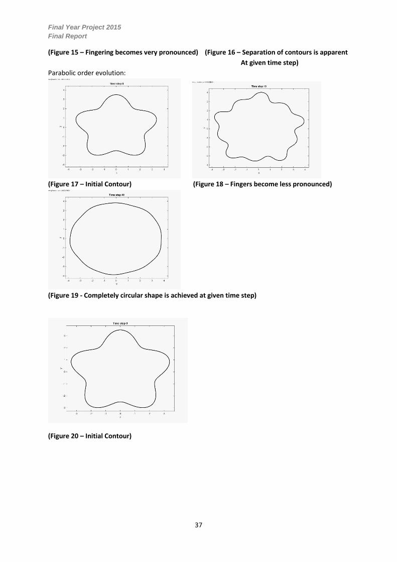
5.1 Influence of Initial Cell Orientation (𝛷)

As discussed in section 4.2, the cell orientation term was altered from a parabolic term to a linear term

whilst still satisfying key requirements. The results of the variance will be qualitatively displayed in this

section.

Parabolic ordered cell orientation –

Linearly ordered cell orientation –

Linear order evolution:

(Figure 13 – Initial contour) (Figure 14 – Contour after a number of time steps,

protrusions are apparent)

(Figure 15 – Fingering becomes very pronounced) (Figure 16 – Separation of contours is apparent

At given time step)


Final Report

17

Parabolic order evolution:

(Figure 17 – Initial Contour) (Figure 18 – Fingers become less pronounced)

(Figure 19 - Completely circular shape is achieved at given time step)

It was observed in figures 13-16 that the linear alignment term created a much higher degree of

‘fingering’ especially in areas of high curvature on the interface. This is as a result of the alignment

term being of first order and thus reducing the relaxation rate to a linear order rather than parabolic.

This displayed a more characteristic growth of the Pseudomonas Aeruginosa colony and was applied

for further testing in the following sections.

The initial phi values were varied as well to more accurate simulate a colony of Pseudomonas

Aeruginosa based on an initial symmetrical contour for each test.


Final Report

18

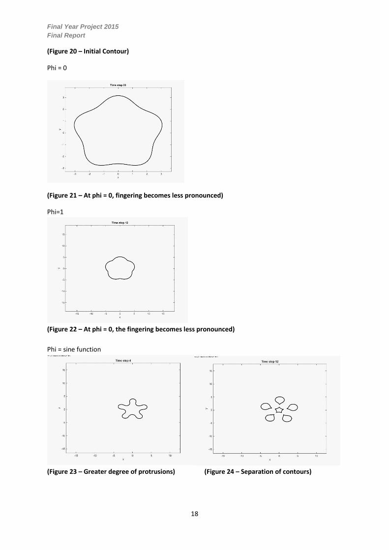
(Figure 20 – Initial Contour)

Phi = 0

(Figure 21 – At phi = 0, fingering becomes less pronounced)

Phi=1

(Figure 22 – At phi = 0, the fingering becomes less pronounced)

Phi = sine function

(Figure 23 – Greater degree of protrusions) (Figure 24 – Separation of contours)


Final Report

19

Whilst maintaining every other variable it can be observed that varying the value of phi has a profound

impact of the computational simulation of the growth of Pseudomonas Aeruginosa. When phi is set

to zero, it can be observed in figure 20 that the initial contour slightly reduces in size and furthermore

becomes perfectly circular. Similarly when phi is set to one the contour becomes almost perfectly

circular with some slight curvature however it increases significantly in area observed in figure 21.

When phi is set to a sine function, its growth pattern is considerably different than the other cases. It

can be seen in figures 22 and 23 that the initial protrusions become more pronounced then break-off

into a colony of six contours. Since the sine function testing most accurately represented experimental

growth of a colony with ‘finger-like’ perturbations, it was chosen to be used for all testing.

5.2 Impact of Bending Rigidity and Surface Tension on Stability (к and ϒ)

For this section, the bending rigidity and surface tension have been switched off and the only forces

in the model are the propulsion forces based on the curvature and orientation of the interface. A

comparison of the various parameters (Alpha Cell, Friction Coefficient and Mass growth rate) are

qualitatively plotted together.

The value chosen for Alpha Cell = 500, Friction Coefficient = 0.4 and Mass growth rate = 20. These

were selected since they elicited the highest degree of colony growth as well as change, exhibiting

similar traits to a colony of Pseudomonas Aeruginosa.

(Figure 25 – Simulation of area with respect to time without bending rigidity and surface tension)

From the figure 25 it can be observed that alpha cell has the greatest effect on the area, followed by

the mass growth rate and lastly the friction coefficient. This suggests that the value of alpha cell has

the most prominent effect on the model equation. Whereas, for the friction coefficient and mass

growth rate, contractive forces have a stronger effect since the propulsive force isn’t as powerful as

the value chosen for alpha cell.

0

500

1000

1500

2000

2500

3000

1

27

53

79

10

5

13

1

15

7

18

3

20

9

23

5

26

1

28

7

31

3

33

9

36

5

39

1

41

7

44

3

46

9

49

5

Dim

ensi

on

less

Are

a

Time Scale

Area of simulation over time without bending rigidity and surface tension

α𝜑=500

𝜂=0.4

𝜇=20


Final Report

20

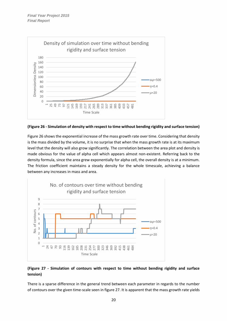
(Figure 26 - Simulation of density with respect to time without bending rigidity and surface tension)

Figure 26 shows the exponential increase of the mass growth rate over time. Considering that density

is the mass divided by the volume, it is no surprise that when the mass growth rate is at its maximum

level that the density will also grow significantly. The correlation between the area plot and density is

made obvious for the value of alpha cell which appears almost non-existent. Referring back to the

density formula, since the area grew exponentially for alpha cell, the overall density is at a minimum.

The friction coefficient maintains a steady density for the whole timescale, achieving a balance

between any increases in mass and area.

(Figure 27 - Simulation of contours with respect to time without bending rigidity and surface

tension)

There is a sparse difference in the general trend between each parameter in regards to the number

of contours over the given time-scale seen in figure 27. It is apparent that the mass growth rate yields

0

20

40

60

80

100

120

140

160

180

12

54

97

39

71

21

14

51

69

19

32

17

24

12

65

28

93

13

33

73

61

38

54

09

43

34

57

48

1

Dim

ensi

on

less

Den

sity

Time Scale

Density of simulation over time without bending rigidity and surface tension

α𝜑=500

𝜂=0.4

𝜇=20

0

1

2

3

4

5

6

7

8

9

12

44

77

09

31

16

13

91

62

18

52

08

23

12

54

27

73

00

32

33

46

36

93

92

41

54

38

46

14

84

No

. of

con

tou

rs

Time Scale

No. of contours over time without bending rigidity and surface tension

α𝜑=500

𝜂=0.4

𝜇=20


Final Report

21

the greatest degree of change in number of contours suggesting it might be the most accurate

representation of the growth of a bacterial colony whereas, the friction coefficient has minimal change

in contours once splits into six difference voids. Alpha cell appears to yield a significant change for the

first 49 time steps however there is minimal change in the contours after that point.

(Figure 28 - Simulation of velocity with respect to time without bending rigidity and surface tension)

The velocity appears to increase for each parameter over time in figure 28. As stated, the oscillations

are representative of voids being removed and separating from the original contour. The link between

the area growth and velocity are again prominent. Alpha cell has a steady increase in area and velocity

over time and so do the friction coefficient and mass growth rate however not to the same degree as

alpha cell.

5.3 Effect of Alignment Forcing Constant (φcell)

The forcing constant, otherwise referred to as alpha cell is the coefficient that sets the magnitude of

the of the orientation dependent force, which was added into the model in the cell self-propulsion

section. The qualitative data surrounding the effect of alpha cell is explored in this section.

-400000

-200000

0

200000

400000

600000

800000

1000000

1

28

55

82

10

9

13

6

16

3

19

0

21

7

24

4

27

1

29

8

32

5

35

2

37

9

40

6

43

3

46

0

48

7

Dim

ensi

on

less

Vel

oci

ty

Time Scale

Velocity of similation over time without bending rigidity and surface tension

α𝜑=500

𝜂=0.4

𝜇=20

0

500

1000

1500

2000

0 200 400 600 800 1000 1200Are

a/In

itia

l Are

a

Time step

Total area of colony over time

Alpha cell = 0.001

Alpha cell = 0.01

Alpha cell = 0.1

Alpha cell = 1

Alpha cell = 10

Alpha cell = 100

Alpha cell = 500


Final Report

22

(Figure 29 – Simulation of the area based on the value of alpha cell)

From figure 29 it can most notably be observed that an overall increase in area occurs for values of

alpha cell that are of a magnitude equal to or above 10. This suggests that at values of α𝜑>10 that the

propulsive orientation forces are much more prominent than the contractive forces.

(Figure 30 - Simulation of the area based on the value of alpha cell)

For values of alpha cell that are below the order of 101, (α𝜑=0.001 to α𝜑=1) as seen on the figure

30 above, there is an initial shrinkage of the total area of the colony. This decrease is followed by

a steady increase in area when the propulsive forces overcome the contractive forces. Overall the

area of each case is parabolic in its nature shown in the plots. For each test, initially the

contractive forces dominate however the propulsive forces prevail in the equation at around 400-

500 time-steps in each case.

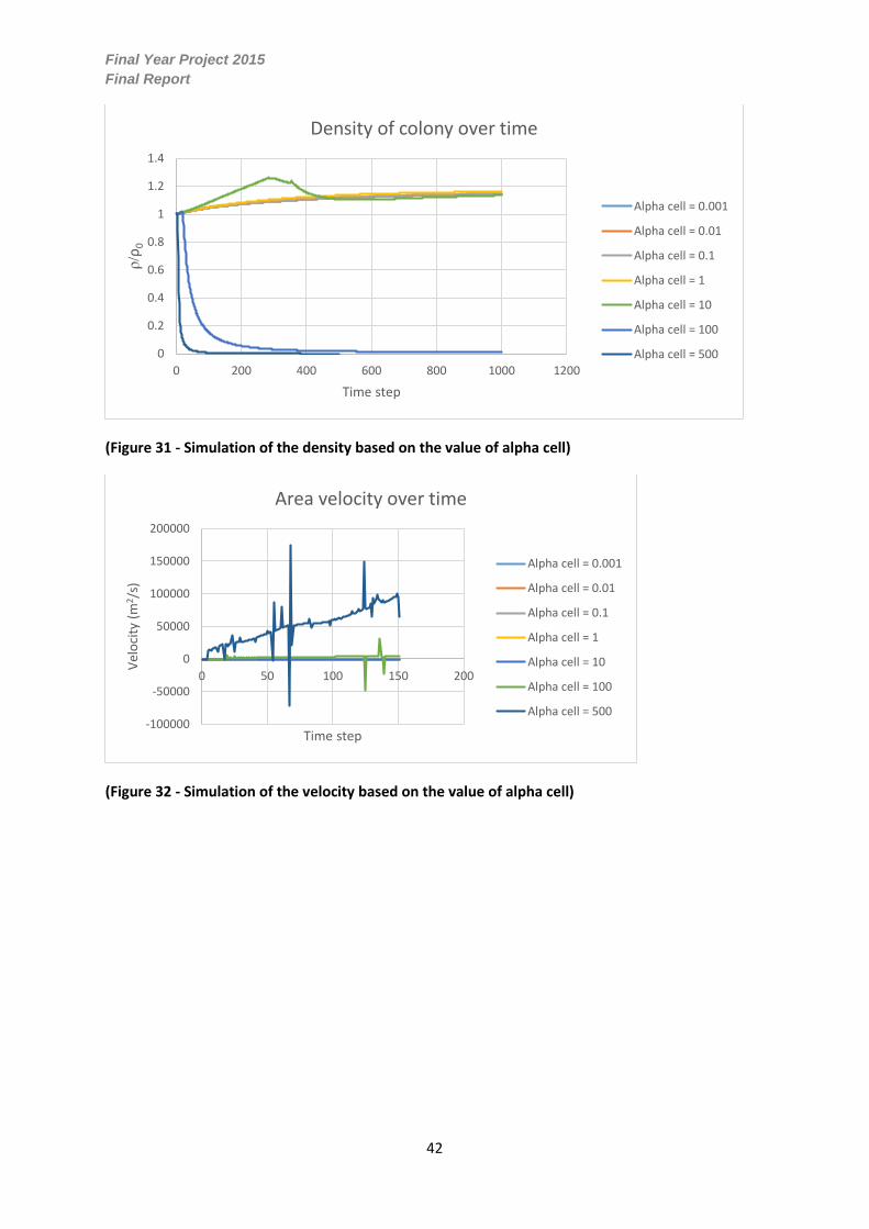
(Figure 31 - Simulation of the density based on the value of alpha cell)

0.92

0.93

0.94

0.95

0.96

0.97

0.98

0.99

1

1.01

0 200 400 600 800 1000 1200

Are

a/In

itia

l Are

a

Time step


Alpha cell = 0.001

Alpha cell = 0.01

Alpha cell = 0.1

Alpha cell = 1

0

0.2

0.4

0.6

0.8

1

1.2

1.4

0 200 400 600 800 1000 1200

ρ/ρ

0

Time step

Density of colony over time

Alpha cell = 0.001

Alpha cell = 0.01

Alpha cell = 0.1

Alpha cell = 1

Alpha cell = 10

Alpha cell = 100

Alpha cell = 500


Final Report

23

The density of the colony increases up to the α𝜑=10 as a result of the mass increasing at a greater

rate than the colonies area observed in figure 31. However for α𝜑=100 to α𝜑=500 there is a rapid

decrease in density for the first two-hundred time-steps followed by a steady convergence to

zero. This significant decrease is a result of the major growth in the colonies area which suggests

that the density will decrease proportionally given a fairly constant mass.

(Figure 32 - Simulation of the velocity based on the value of alpha cell)

From figure 32 there is a significant increase in velocity for α𝜑=100 to α𝜑=500, eluding to the

relationship between the area and velocity. The oscillations are resultant from the removal of

separated voids and are therefore false values. Overall at α𝜑=100 to α𝜑=500, the velocity of the

colony increases linearly similarly to the area.

(Figure 33 - Simulation of the contours based on the value of alpha cell)

-100000

-50000

0

50000

100000

150000

200000

0 50 100 150 200

Vel

oci

ty (

m2/s

)

Time step

Area velocity over time

Alpha cell = 0.001

Alpha cell = 0.01

Alpha cell = 0.1

Alpha cell = 1

Alpha cell = 10

Alpha cell = 100

Alpha cell = 500

0

1

2

3

4

5

6

7

0 200 400 600 800 1000 1200

Nu

mb

er o

f co

nto

urs

Time step

Number of contours over time

Alpha cell = 0.001

Alpha cell = 0.01

Alpha cell = 0.1

Alpha cell = 1

Alpha cell = 10

Alpha cell = 100

Alpha cell = 500


Final Report

24

It can be seen that voids are not created till alpha cell reaches 101 and of higher order in figure 33.

The frequency of voids forming and removing becomes more apparent as alpha cell increases.

Alpha cell has a very insignificant effect on growth for any values less than 1, however when the

selected value is of order 101 or above there is a distinguishable difference in each curve from one

another. It can be seen that growth becomes increasingly rapid as alpha cell becomes the dominant

forcing term in the model equation and the effects of the contractive forces are minimalized.

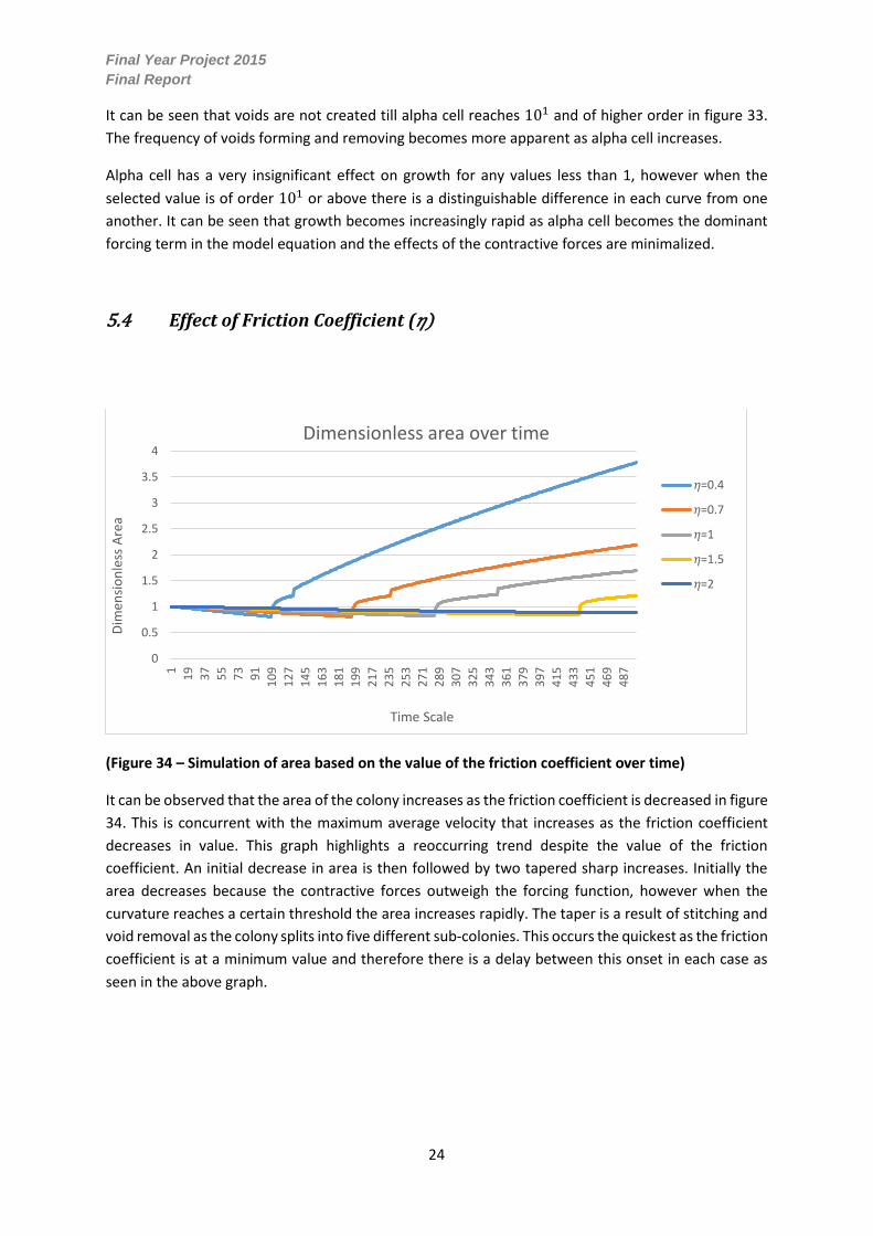
5.4 Effect of Friction Coefficient (𝜂)

(Figure 34 – Simulation of area based on the value of the friction coefficient over time)

It can be observed that the area of the colony increases as the friction coefficient is decreased in figure

34. This is concurrent with the maximum average velocity that increases as the friction coefficient

decreases in value. This graph highlights a reoccurring trend despite the value of the friction

coefficient. An initial decrease in area is then followed by two tapered sharp increases. Initially the

area decreases because the contractive forces outweigh the forcing function, however when the

curvature reaches a certain threshold the area increases rapidly. The taper is a result of stitching and

void removal as the colony splits into five different sub-colonies. This occurs the quickest as the friction

coefficient is at a minimum value and therefore there is a delay between this onset in each case as

seen in the above graph.

0

0.5

1

1.5

2

2.5

3

3.5

4

1

19

37

55

73

91

10

9

12

7

14

5

16

3

18

1

19

9

21

7

23

5

25

3

27

1

28

9

30

7

32

5

34

3

36

1

37

9

39

7

41

5

43

3

45

1

46

9

48

7

Dim

ensi

on

less

Are

a

Time Scale

Dimensionless area over time

𝜂=0.4

𝜂=0.7

𝜂=1

𝜂=1.5

𝜂=2


Final Report

25

(Figure 35 - Simulation of density based on the value of the friction coefficient over time)

A similar trend can also be observed in the density over the given timescale for each case displayed in

figure 35. A linear increase is then met by a slight linear decrease followed by a parabolic fall then rise.

A comparison can be drawn between the initial rise and the area plot. The initial decrease in total area

consequentially allows for a correlated increase in density. The density subtly decreases as a result of

the sharp increase in area between 106 and 148 in the timescale corresponding to a friction coefficient

of 0.4.

(Figure 36 - Simulation of contours based on the value of the friction coefficient over time)

The maximum number of contours is equivalent to one more than the number of initial perturbations

in the initial model (phi as a sin function). The growth pattern yields five separate voids and an initial

0

0.2

0.4

0.6

0.8

1

1.2

1.4

1

22

43

64

85

10

6

12

7

14

8

16

9

19

0

21

1

23

2

25

3

27

4

29

5

31

6

33

7

35

8

37

9

40

0

42

1

44

2

46

3

48

4

Dim

ensi

on

less

Den

sity

Timescale


𝜂=0.4

𝜂=0.7

𝜂=1

𝜂=1.5

𝜂=2

0

1

2

3

4

5

6

7

1

18

35

52

69

86

10

3

12

0

13

7

15

4

17

1

18

8

20

5

22

2

23

9

25

6

27

3

29

0

30

7

32

4

34

1

35

8

37

5

39

2

40

9

42

6

44

3

46

0

47

7

49

4

No

. of

con

tou

rs

Time Scale

No. of contours in colony over time

𝜂=0.4

𝜂=0.7

𝜂=1

𝜂=1.5

𝜂=2


Final Report

26

void that becomes removed as it shrinks in size which corresponds from six contours to five as seen in

figure 36. The friction coefficient effects the rates at which this occurs. A larger friction coefficient

equivalent to the value of two does not reach the stage of splitting into separate contours since the

growth rate is almost insignificant.

(Figure 37 - Simulation of velocity based on the value of the friction coefficient over time)

The two distinct rises and peaks in the velocity correspond to the initial contour splitting into six voids

causing a large impulse and the initial void being removed as seen in figure 37.

5.5 Effect of Specific Mass Growth Rate (𝜇)

(Figure 38 - Simulation of area based on the value of the mass growth rate over time)

-1000

0

1000

2000

3000

4000

5000

1

27

53

79

10

5

13

1

15

7

18

3

20

9

23

5

26

1

28

7

31

3

33

9

36

5

39

1

41

7

44

3

46

9

49

5

Vel

oci

ty (

Are

a/s)

Time Scale

Velocity of colony over time

𝜂=0.4

𝜂=0.7

𝜂=1

𝜂=1.5

𝜂=2

0

20

40

60

80

100

120

140

160

1

22

43

64

85

10

6

12

7

14

8

16

9

19

0

21

1

23

2

25

3

27

4

29

5

31

6

33

7

35

8

37

9

40

0

42

1

44

2

46

3

48

4

Are

a

Time Scale

Dimensionless Area over time based on mass growth rate

𝜇=0.1

𝜇=1

𝜇=10

𝜇=20


Final Report

27

(Figure 39 - Simulation of density based on the value of the mass growth rate over time)

(Figure 40 - Simulation of contours based on the value of the mass growth rate over time)

0

50

100

150

2001

20

39

58

77

96

11

5

13

4

15

3

17

2

19

1

21

0

22

9

24

8

26

7

28

6

30

5

32

4

34

3

36

2

38

1

40

0

41

9

43

8

45

7

47

6

49

5

Dim

ensi

on

less

den

sity

Time Scale

Dimensionless density over time based on mass growth rate

𝜇=0.1 𝜇=1 𝜇=10 𝜇=20

0

50

100

150

200

1

20

39

58

77

96

11

5

13

4

15

3

17

2

19

1

21

0

22

9

24

8

26

7

28

6

30

5

32

4

34

3

36

2

38

1

40

0

41

9

43

8

45

7

47

6

49

5

No

. of

con

tou

rs

Time Scale

No. of contours over time scale based on mass growth rate

𝜇=0.1 𝜇=1 𝜇=10 𝜇=20


Final Report

28

(Figure 41 - Simulation of velocity based on the value of the mass growth rate over time)

It can be observed in the above figures that for mass growth rate values less than or equal to one

there is no significant changes in the colonies area however once 𝜇 is increased to an order of

magnitude of 101 there is an obvious exponential growth in the colonies area over time. This is

characteristic of an actual pseudomonas colony. This observation can be seen in not only the area but

the density, number of contours and velocity as well closely linking the mass growth rate of 𝜇 equals

20 to an actual colony. As the mass growth rate is increased the density increases exponentially as

seen in the corresponding graph. This causes a negative exponential increase in the forcing function

when the curvature is less than zero. This causes significant contraction allowing for many fingers to

be birthed and joined to create contours which is highlighted in the number of contours graph. At its

maximum value the mass growth rate simulation most accurately represented the growth of an actual

colony as compared to the other variables that were tested.

6. FUTURE WORK

6.1 Revised Model

Based on the parameters tested in section 5, to most accurately represent a growth of Pseudomonas

Aeruginosa:

The mass growth rate should be maximized to an order of 101.

Friction coefficient should be lowered to the minimum allowable value of 0.4.

Alpha cell should either remain at an order of 101 or be increased to a higher order.

Bending Rigidity and Surface Tension should remain active.

The cell orientation equation should remain a linear term, however it should be updated to

reduce the contour separation seen in testing.

-150000

-100000

-50000

0

50000

100000

150000

1

22

43

64

85

10

6

12

7

14

8

16

9

19

0

21

1

23

2

25

3

27

4

29

5

31

6

33

7

35

8

37

9

40

0

42

1

44

2

46

3

48

4

Dim

ensi

on

less

Vel

oci

ty

Time Scale

Dimensionless velocity over time based on mass growth rate

𝜇=0.1 𝜇=1 𝜇=10 𝜇=20


Final Report

29

6.2 Further Suggestions

Nodal redistribution could be made more efficient to reduce computational time running the

code.

Void removal could be enhanced to minimize the change of area and velocity of the contour.

A new code separating the areas of the separate contours into a variety of plots would give

the user a more accurate depiction and the various areas on the colony.

Further testing could be completed on the other parameters such as: constant baseline force,

force-vs-curvature coefficient, baseline relaxation time, exponential forcing function

coefficient and initial mass.

Test computational results experimentally in a variety of conditions

Apply gained knowledge and understanding to mitigate the spread of and inhibit the growth

of Pseudomonas Aeruginosa.

7. CONCLUSIONS

A summary of section five and the effects of the parameters varied is as follows:

Cell orientation yields a more characteristic growth of Pseudomonas Aeruginosa when it is of

a linear order rather than parabolic due to a much higher degree of ‘fingering.’

Setting the value of phi to a sine function compared with an integer created a much higher

degree of ‘fingering’ and separated contours.

When bending rigidity and surface tension were set to zero, Alpha cell proved to exhibit the

highest growth in area since no restrictive forces restricted growth. Mass growth rate

exhibited an exponential increase in density and a sparseness in the number of contours over

the time period. Friction coefficient had a minimal impact on growth.

For Alpha cell, it was observed that values of an order less than 101had an insignificant impact

on growth and other measurable quantities. However as alpha cell was increased past

101there was a rapid increase in area growth and the number of contours. This was a result

of alpha cell becoming the most dominant term in the model equation.

For the friction coefficient, as the value was increased, a slower growth rate was observed

and as the value decreased there was a more rapid rate of growth. Due to the restricted range

of integers that could be tested, the friction coefficient had a minimal impact on growth.

For specific mass growth rate, similarly to alpha cell, an insignificant difference was

qualitatively observed in measurable parameters for values less than of order of magnitude.

101. Based on the formulation, density increases exponentially as the mass growth rate is

increased past 101. The area and number of contours follow a similar trend. At its maximum

value the mass growth rate simulation most accurately represented the growth of an actual

colony as compared to the other variables that were tested.


Final Report

30

8. ACKNOWLEDGEMENTS I would like to thank Dr. Prabhakar Ranganathan for his supervision, direction and assistance

throughout the project. I would also like to acknowledge Max Zadnik and Josh Sweeney whose work

we were following on from, as well as Amarender Nagilla for answering any questions we had.

9. REFERENCES

Gloag, E, Turnbull, L, Huang, A, Vallotton, P, Wang, H, Nolan, L, Mililli, L, Hunt, C, Lu, J, Osvath, S,

Monahan, L, Cavaliere, R, Charles, I, Wand, M, Gee, M, Ranganathan, P, Whitchurch, C 2013, ‘Self-

organisation of bacterial biofilms is facilitated by extracellular DNA’, Proceedings of the National

Academy of Sciences, vol. 110 no. 28

Mark, S, Shlomovitz, R, Gov, N, Poujade, M, Grasland-Mongrain, E & Silbersan, P 2010, ‘Physical Model

of the Dynamic Instability in an Expanding Cell Culture’, Biophysical Journal, vol. 98, no. 3, pp. 361-370

Ranganathan, PR, 2014. Mechanobiology of construction and operation of interstitial traffic networks

in Pseudomonas aeruginosa. Complex Flows of Complex Fluids. Department of Mechanical &

Aerospace Engineering: Monash University.

Ranganathan, PR, 2015. A model for the advancing edge of a monolayer of motile rod-shaped bacteria.

FYP. Engineering: Monash University.

Saffman, P, Taylor, G 1958, ‘The Penetration of a Fluid into a Porous Medium or Hele-Shaw Cell

Containing a More Viscous Liquid’, Proceedings of the Royal Society of London. Series A, Mathematical

and Physical Sciences, vol. 245 no 1242, pp. 312-329

Sweeney J, Zadnik M, 2014. FLUID MECHANICS OF BACTERIAL INFECTIONS. FYP. Engineering: Monash

University.


Final Report

31

10. APPENDICES

Appendix 1: Computational Simulation based on varying Alpha Cell

α𝜑=0.001 α𝜑=0.01

α𝜑=0.1 α𝜑=1

α𝜑=10 α𝜑=100


Final Report

32

α𝜑=500

Appendix 2: Model equations used


Final Report

33

Appendix 3: Figures and graphs

(Figure 2 – Pre-stitching computational simulation)

(Figure 3 – Post-stitching computational simulation)


Final Report

34

(Figure 4 – Pre void removal simulation) (Figure 5 – Post void removal simulation)

(Figure 6 – illustration of relaxation is at a maximum when curvature is small)

(Figure 7 – illustration that relaxation rate reduces to zero as cells are close to aligned)


Final Report

35

(Figure 8 – Regular computational simulation depicting voids at a given time step)

(Figure 9 – Top contour from figure 8 selected for contour extraction)

(Figure 10 – An initially symmetrical contour)


Final Report

36

(Figure 11 – Relatively symmetrical after a number of time-steps)

(Figure 12 – Computational anomalies are made obvious as all symmetry is non-apparent)

(Figure 13 – Initial contour) (Figure 14 – Contour after a number of time steps,

protrusions are apparent)


Final Report

37

(Figure 15 – Fingering becomes very pronounced) (Figure 16 – Separation of contours is apparent

At given time step)

Parabolic order evolution:

(Figure 17 – Initial Contour) (Figure 18 – Fingers become less pronounced)

(Figure 19 - Completely circular shape is achieved at given time step)

(Figure 20 – Initial Contour)


Final Report

38

(Figure 21 – At phi = 0, fingering becomes less pronounced)

(Figure 22 – At phi = 0, the fingering becomes less pronounced)

(Figure 23 – Greater degree of protrusions) (Figure 24 – Separation of contours)


Final Report

39

(Figure 25 – Simulation of area with respect to time without bending rigidity and surface tension)

(Figure 26 - Simulation of density with respect to time without bending rigidity and surface tension)

0

500

1000

1500

2000

2500

30001

27

53

79

10

5

13

1

15

7

18

3

20

9

23

5

26

1

28

7

31

3

33

9

36

5

39

1

41

7

44

3

46

9

49

5

Dim

ensi

on

less

Are

a

Time Scale

Area of simulation over time without bending rigidity and surface tension

α𝜑=500

𝜂=0.4

𝜇=20

0

20

40

60

80

100

120

140

160

180

12

54

97

39

71

21

14

51

69

19

32

17

24

12

65

28

93

13

33

73

61

38

54

09

43

34

57

48

1

Dim

ensi

on

less

Den

sity

Time Scale

Density of simulation over time without bending rigidity and surface tension

α𝜑=500

𝜂=0.4

𝜇=20


Final Report

40

(Figure 27 - Simulation of contours with respect to time without bending rigidity and surface

tension)

(Figure 28 - Simulation of velocity with respect to time without bending rigidity and surface tension)

0

1

2

3

4

5

6

7

8

9

12

44

77

09

31

16

13

91

62

18

52

08

23

12

54

27

73

00

32

33

46

36

93

92

41

54

38

46

14

84

No

. of

con

tou

rs

Time Scale

No. of contours over time without bending rigidity and surface tension

α𝜑=500

𝜂=0.4

𝜇=20

-400000

-200000

0

200000

400000

600000

800000

1000000

1

28

55

82

10

9

13

6

16

3

19

0

21

7

24

4

27

1

29

8

32

5

35

2

37

9

40

6

43

3

46

0

48

7

Dim

ensi

on

less

Vel

oci

ty

Time Scale

Velocity of similation over time without bending rigidity and surface tension

α𝜑=500

𝜂=0.4

𝜇=20


Final Report

41

(Figure 29 – Simulation of the area based on the value of alpha cell)

(Figure 30 - Simulation of the area based on the value of alpha cell)

0

200

400

600

800

1000

1200

1400

1600

1800

0 200 400 600 800 1000 1200

Are

a/In

itia

l Are

a

Time step


Alpha cell = 0.001

Alpha cell = 0.01

Alpha cell = 0.1

Alpha cell = 1

Alpha cell = 10

Alpha cell = 100

Alpha cell = 500

0.92

0.93

0.94

0.95

0.96

0.97

0.98

0.99

1

1.01

0 200 400 600 800 1000 1200

Are

a/In

itia

l Are

a

Time step


Alpha cell = 0.001

Alpha cell = 0.01

Alpha cell = 0.1

Alpha cell = 1


Final Report

42

(Figure 31 - Simulation of the density based on the value of alpha cell)

(Figure 32 - Simulation of the velocity based on the value of alpha cell)

0

0.2

0.4

0.6

0.8

1

1.2

1.4

0 200 400 600 800 1000 1200

ρ/ρ

0

Time step


Alpha cell = 0.001

Alpha cell = 0.01

Alpha cell = 0.1

Alpha cell = 1

Alpha cell = 10

Alpha cell = 100

Alpha cell = 500

-100000

-50000

0

50000

100000

150000

200000

0 50 100 150 200

Vel

oci

ty (

m2 /

s)

Time step

Area velocity over time

Alpha cell = 0.001

Alpha cell = 0.01

Alpha cell = 0.1

Alpha cell = 1

Alpha cell = 10

Alpha cell = 100

Alpha cell = 500


Final Report

43

(Figure 33 - Simulation of the contours based on the value of alpha cell)

(Figure 34 – Simulation of area based on the value of the friction coefficient over time)

0

1

2

3

4

5

6

7

0 200 400 600 800 1000 1200

Nu

mb

er o

f co

nto

urs

Time step

Number of contours over time

Alpha cell = 0.001

Alpha cell = 0.01

Alpha cell = 0.1

Alpha cell = 1

Alpha cell = 10

Alpha cell = 100

Alpha cell = 500

0

0.5

1

1.5

2

2.5

3

3.5

4

1

19

37

55

73

91

10

9

12

7

14

5

16

3

18

1

19

9

21

7

23

5

25

3

27

1

28

9

30

7

32

5

34

3

36

1

37

9

39

7

41

5

43

3

45

1

46

9

48

7

Dim

ensi

on

less

Are

a

Time Scale

Dimensionless area over time

𝜂=0.4

𝜂=0.7

𝜂=1

𝜂=1.5

𝜂=2


Final Report

44

(Figure 35 - Simulation of density based on the value of the friction coefficient over time)

(Figure 36 - Simulation of contours based on the value of the friction coefficient over time)

0

0.2

0.4

0.6

0.8

1

1.2

1.4

1

22

43

64

85

10

6

12

7

14

8

16

9

19

0

21

1

23

2

25

3

27

4

29

5

31

6

33

7

35

8

37

9

40

0

42

1

44

2

46

3

48

4

Dim

ensi

on

less

Den

sity

Timescale


𝜂=0.4

𝜂=0.7

𝜂=1

𝜂=1.5

𝜂=2

0

1

2

3

4

5

6

7

1

18

35

52

69

86

10

3

12

0

13

7

15

4

17

1

18

8

20

5

22

2

23

9

25

6

27

3

29

0

30

7

32

4

34

1

35

8

37

5

39

2

40

9

42

6

44

3

46

0

47

7

49

4

No

. of

con

tou

rs

Time Scale

No. of contours in colony over time

𝜂=0.4

𝜂=0.7

𝜂=1

𝜂=1.5

𝜂=2


Final Report

45

(Figure 37 - Simulation of velocity based on the value of the friction coefficient over time)

(Figure 38 - Simulation of area based on the value of the mass growth rate over time)

-1000

0

1000

2000

3000

4000

5000

1

27

53

79

10

5

13

1

15

7

18

3

20

9

23

5

26

1

28

7

31

3

33

9

36

5

39

1

41

7

44

3

46

9

49

5

Vel

oci

ty (

Are

a/s)

Time Scale

Velocity of colony over time

𝜂=0.4

𝜂=0.7

𝜂=1

𝜂=1.5

𝜂=2

0

20

40

60

80

100

120

140

160

1

22

43

64

85

10

6

12

7

14

8

16

9

19

0

21

1

23

2

25

3

27

4

29

5

31

6

33

7

35

8

37

9

40

0

42

1

44

2

46

3

48

4

Are

a

Time Scale

Dimensionless Area over time based on mass growth rate

𝜇=0.1

𝜇=1

𝜇=10

𝜇=20


Final Report

46

(Figure 39 - Simulation of density based on the value of the mass growth rate over time)

(Figure 40 - Simulation of contours based on the value of the mass growth rate over time)

0

50

100

150

2001

20

39

58

77

96

11

5

13

4

15

3

17

2

19

1

21

0

22

9

24

8

26

7

28

6

30

5

32

4

34

3

36

2

38

1

40

0

41

9

43

8

45

7

47

6

49

5

Dim

ensi

on

less

den

sity

Time Scale

Dimensionless density over time based on mass growth rate

𝜇=0.1 𝜇=1 𝜇=10 𝜇=20

0

50

100

150

200

1

20

39

58

77

96

11

5

13

4

15

3

17

2

19

1

21

0

22

9

24

8

26

7

28

6

30

5

32

4

34

3

36

2

38

1

40

0

41

9

43

8

45

7

47

6

49

5

No

. of

con

tou

rs

Time Scale

No. of contours over time scale based on mass growth rate

𝜇=0.1 𝜇=1 𝜇=10 𝜇=20


Final Report

47

(Figure 41 - Simulation of velocity based on the value of the mass growth rate over time)

-150000

-100000

-50000

0

50000

100000

150000

1

22

43

64

85

10

6

12

7

14

8

16

9

19

0

21

1

23

2

25

3

27

4

29

5

31

6

33

7

35

8

37

9

40

0

42

1

44

2

46

3

48

4

Dim

ensi

on

less

Vel

oci

ty

Time Scale

Dimensionless velocity over time based on mass growth rate

𝜇=0.1 𝜇=1 𝜇=10 𝜇=20

joel voigt - 24227730 - finalyearreport-mec4401

Documents