johan janson olstam andreas tapani - diva portal673977/fulltext01.pdf · johan janson olstam och...

VTI m

edde

land

e 96

0A •

2004 Comparison of Car-following

models

Johan Janson OlstamAndreas Tapani

VTI meddelande 960A · 2004

Comparison of Car-following models

Johan Janson OlstamAndreas Tapani

Publisher: Publication:

VTI meddelande 960A

Published: 2004

Project code: 40503 and 40485

SE-581 95 Linköping Sweden Project: Development of the VTI rural traffic simula-tion model and Simulated traffic for the VTI driving simulator

Author: Sponsor: Johan Janson Olstam and Andreas Tapani Swedish National Road Administration

Title: Comparison of Car-following models

Abstract

Traffic simulation is an often used tool in the study of traffic systems. A traffic simulation model consists of several sub-models; each handles one specific task in the simulation. These sub-models include, among others, car-following. This model controls the interactions with the preceding vehicle in the same lane.

This paper compares and describes the car-following models used in the four traffic micro-simulation software packages AIMSUN, MITSIM, VISSIM, and the Fritzsche car-following model. A variant of the Fritzsche model is used in the software tool Parmics. Paramics exists in two versions. The differences between the Car-following models used in these versions and the Fritzsche car-following model is however unknown. Both similarities and differences between the models as well as model’s individual properties are clarified.

Two of the four models, the Fritzsche model and the model included in VISSIM, have a similar approach to car-following, whereas the other two models have fundamentally different approaches. However, the resulting following behaviors of the models show similarities even though the car-following approaches are different.

ISSN: Language: No. of pages: 0347-6049 English 36 + 2 Appendices

Utgivare: Publikation:

VTI meddelande 960A

Utgivningsår: 2004

Projektnummer: 40503 och 40485

581 95 Linköping Projektnamn: Vidareutveckling av VTI:s trafiksimulerings-modell för landsväg och simulerad trafik till VTI:s körsimulator

Författare: Uppdragsgivare: Johan Janson Olstam och Andreas Tapani Vägverket

Titel: Jämförelse av car-followingmodeller

Referat

Trafiksimulering är ett vanligt verktyg för studier av trafiksystem. En trafiksimuleringsmodell består av flera delmodeller som var och en behandlar en specifik del i simuleringen. En av dessa del-modeller är en modell för car-following. Denna modell beskriver en förares interaktion med det fram-förvarande fordonet i samma körfält.

Denna rapport jämför och beskriver car-followingmodellerna som används i de tre mikrosimule-ringsprogramvarorna AIMSUN, MITSIM, VISSIM och Fritzsche’s car-following modell. En variant av Fritzsche’s modell används i programmet Paramics. Rapporten tar både upp likheter och skillnader mellan modellerna samt även de olika modellernas individuella egenskaper.

Två av de fyra modellerna, Fritzsche's modell och modellen i VISSIM liknar varandra medan de andra två modellerna har helt andra utgångspunkter för modelleringen av car-followingbeteende. De olika modellernas följandebeteende uppvisar dock likheter även om deras modelleringsansatser vad gäller car-following skiljer sig åt.

ISSN: Språk: Antal sidor: 0347-6049 Engelska 36 + 2 Bilagor

Preface This comparison of Car-following models has been conducted within the projects “Development of the VTI rural traffic simulation model” and “Simulated traffic for the VTI driving simulator”. Special thanks to Mikael Adlers, VTI, who have reviewed the contents of this report; and to Jan Lundgren, Linköping Institute of Technology, and Urban Björketun, VTI, for their invaluable comments. Linköping May 2004 Pontus Matstoms Project Manager

VTI meddelande 960A

VTI meddelande 960A

Contents Page Summary 5

Sammanfattning 7

1 Introduction 9

2 Outline 11

3 Car-following 12 3.1 Classification of car-following models 13 3.2 Model properties 14 3.3 AIMSUN 16 3.4 MITSIM 17 3.5 Fritzsche (Paramics) 18 3.6 VISSIM 21

4 Comparison of car-following models 25 4.1 Test 25 4.2 Discussion 31

5 Conclusions 34

6 References 35

Appendices Appendix 1 Overview of studied micro-simulation software Appendix 2 Simulation parameters

VTI meddelande 960A

Figures Page Figure 1 Car- following notation 12

Figure 2 A psycho-physical car-following model 14 Figure 3 The different thresholds and regimes in the Fritzsche car-following model 20 Figure 4 The different thresholds and regimes in the Wiedemann car-following model 22 Figure 5 Speed, acceleration and distance gap for the AIMSUN car-following model 26 Figure 6 Speed, acceleration and distance gap for the MITSIM car-following model 27 Figure 7 Speed, acceleration and distance gap for the Fritzsche (Paramics) car-following model 28 Figure 8 Speed, acceleration and distance gap for the VISSIM car-following model 29

Figure 9 Speed of follower and leader during the driving course of events 30 Figure 10 Front to rear distance between follower and leader during the driving course of events. 30

VTI meddelande 960A

Comparison of Car-following models

by Johan Janson Olstam and Andreas Tapani Swedish National Road and Transport Research Institute (VTI) SE-581 95 Linköping Sweden Summary Traffic simulation is an often used tool in the study of traffic systems. A traffic simulation model consists of several sub-models; each handles one specific task in the simulation. These sub-models include, among others, car-following. This model describes the interactions with the preceding vehicle in the same lane. This paper compares and describes the car-following models used in the three traffic micro-simulation software packages AIMSUN, MITSIM, VISSIM, and the Fritzsche car-following model. A variant of the Fritzsche model is used in the software tool Paramics. Both similarities and differences between the models as well as model’s individual properties are clarified. Micro-simulation of traffic as a tool for investigating traffic systems has increased in popularity over the last decades. The number of simulation models is very large and the simulation approach utilized in these models is to a large extent differentiated. This gives rise to a need for comparison of traffic micro-simulation models. This work presents and compares the car-following logic utilized in four of today’s most popular traffic micro-simulation programs: AIMSUN, MITSIM, Paramics (The Fritzsche car-following model is studied) and VISSIM.

Traffic micro-simulation models consider individual vehicle’s interactions with other vehicles and the road network. The models are commonly built up by sub models controlling specific tasks in the simulation process. The car-following model one of the most important sub models, used in all programs. A car-following model controls the driver’s behavior with respect to the preceding vehicle in the same lane.

Car-following models are commonly classified into classes depending on the utilized logic. Such model classes include:

• Gazis-Herman-Rothery models (GHR). These models state that the following vehicle’s acceleration is proportional to the speed of the follower, the speed difference between follower and leader and the space headway.

• Safety-distance models. Safety distance models are based on the assump-tion that the follower always keeps a safe distance to the vehicle in front.

• Psycho-physical car-following models. These models use thresholds for, e.g., the minimum speed difference between follower and leader perceived by the follower.

The car-following model of AIMSUN is of safety distance type. MITSIM’s car-following model uses GHR-type logic and the Fritzsche model and the model incorporated in VISSIM can be classified as psycho-physical models.

Traffic micro-simulation models are commonly used to estimate macroscopic traffic measures. The most important property of the car-following models used in

VTI meddelande 960A 5

such applications is therefore that the models are able to produce representative macroscopic traffic measures. Models used in applications were microscopic vehicle movements are important, place additional requirements on the car-following modeling.

In order to compare and enlighten the car-following behavior of the four programs a numerical test of the models has been carried out. The car-following equations of each of the four models have been implemented in MATLAB. Each models follower equation has then been allowed to act on the same driving course of events of an artificial leader. The outcome of the test was the follower’s driving course of events for all four models.

The VISSIM and the Fritzsche models showed similar follower behaviors. This was readily explained by the fact that these models belonged to the same model class. The follower’s reaction time differed between the four models. The magnitude of the follower’s reaction was also unique for each model.

All traffic micro-simulation models use a very large number of parameters that have to be calibrated in order to achieve representative results. The calibration work increases fast with the number of parameters. It is therefore desirable to keep the number of parameters as small as possible. A car-following model must however contain parameters that allow both the reaction time and the magnitude of the reaction to be adjusted. Of the studied models VISSIM and the Fritzsche models contain the largest number of parameters and AIMSUN is the model with the smallest number of parameters.

The test conducted in this work used a simple artificial driving course of events for the leader vehicle. A more thorough study would require driving course of events measured in real traffic. Interesting next steps on the path outlined by this work is to analyze stability properties of car-following models by studying car-following in platoons of more than two vehicles.

6 VTI meddelande 960A

Jämförelse av car-followingmodeller

av Johan Janson Olstam and Andreas Tapani Statens väg- och transportforskningsinstitut (VTI) SE-581 95 Linköping Sammanfattning Trafiksimulering är ett vanligt verktyg för studier av trafiksystem. En trafik-simuleringsmodell består av flera delmodeller som var och en behandlar en specifik del i simuleringen. En av dessa delmodeller är en modell för car-following. Denna modell beskriver en förares interaktion med det framför-varande fordonet i samma körfält. Denna rapport jämför och beskriver car-followingmodellerna som används i de tre mikrosimulerings-programvarorna AIMSUN, MITSIM, VISSIM samt Fritzsche’s car-followingmodell. En variant av Fritzsche’s modell används i programmet Paramics. Rapporten tar både upp likheter och skillnader mellan modellerna samt de olika modellernas individuella egenskaper. Mikrosimulering av trafik har blivit ett mycket populärt verktyg för studier av trafiksystem. Det finns många olika modeller och program och deras simulerings-ansats skiljer sig till stora delar åt. Det finns därför ett stort behov av jämförelser av olika trafiksimuleringsmodeller. Detta arbete presenterar och jämför car-followinglogiken som används i fyra av dagens mest populära trafiksimulerings-program: AIMSUN, MITISM, Paramics (Fritzsche’s modell studeras) och VISSIM.

En trafiksimuleringsmodell behandlar individuella fordons interaktioner med andra fordon och vägen. Modellerna är vanligtvis uppbyggda av delmodeller som styr olika delar i simuleringen. Car-folllowingmodellen är en av de viktigaste modellerna och används i princip i alla program. En car-followingmodell styr förares beteende vad det gäller interaktionen med framförvarande fordon i samma körfält.

Car-followingmodeller delas ofta in i klasser beroende på vilken typ av logik de använder. De kan till exempel delas in i följande klasser:

• Gazis-Herman-Rothery-modeller (GHR). En GHR modell antar att ett följ-ande fordons acceleration är proportionerlig mot ledarens hastighet samt hastighetsskillnaden och avståndet dem emellan.

• Säkerhetsavståndsmodeller. En säkerhetsavståndsmodell baseras på antagandet att följaren alltid försöker hålla ett säkert avstånd till framför-varande fordon.

• Psycho-fysiska car-followingmodeller. Denna klass av modeller använder sig av olika gränser för till exempel den minsta hastighetsskillnad mellan ledare och följare som följaren kan uppfatta.

Den car-followingmodell som används i AIMSUN kan klassificeras som en säker-hetsavståndsmodell. MITSIM använder en GHR modell medan Fritzsche’s modell och den modell som används i VISSIM är psycho-fysiska modeller.

Trafiksimuleringsmodeller används oftast för att få fram makroskopiska trafikmått. Den viktigaste egenskapen för en trafiksimuleringsmodell som an-


vänds i detta syfte är att modellen kan skapa representativa makroskopiska trafik-mått. Trafiksimuleringsmodeller som däremot används för att skapa mikro-skopiska fordonsrörelser som utdata, ställer högre krav på den car-following-modell som används.

För att jämföra och studera car-followingbeteendet hos de fyra olika mo-dellerna har ett numeriskt test genomförts. Modellernas car-followingekvationer har implementerats i MATLAB. Varje modells car-followingmodell har sedan fått reagera på samma körförlopp hos ett artificiellt ledarfordon. Utdata från testet blir följarens reaktioner på ledarens körförlopp.

VISSIM’s och Fritzsche’s modell uppvisar liknande följandebeteende, vilket är naturligt då de tillhör samma modellklass. Följarens reaktionstid och hur kraftigt följaren reagerade varierade mellan de fyra modellerna.

Alla trafiksimuleringsmodeller använder ett stort antal olika parametrar som måste kalibreras för att uppnå tillförlitliga resultat. Kalibreringsarbetet ökar kraftigt med antalet parametrar. Det är därför önskvärt att hålla antalet parametrar så lågt som möjligt. En car-followingmodell måste dock innehålla parametrar så att både reaktionstid och reaktionsstyrka kan justeras. Bland de studerade modellerna så innehåller VISSIM och Fritzsche’s modell flest parametrar. AIMSUN är den modell som innehåller minst antal parametrar.

Det test som genomfördes inom ramen för detta arbete utgick från ett artificiellt körförlopp. En fördjupad studie kräver körförlopp uppmätta i verkligheten. Ett intressant nästa steg kan vara att studera car-followingbeteende i fordonskolonner.


1 Introduction Micro-simulation of traffic as a tool for investigating traffic systems has increased in popularity over the last decades. A large portion of this rise in popularity can be tracked back to the rapid development in the personal computer area. Fast PCs have made it possible to develop advanced traffic micro-simulation software packages. Today, the number of simulation models is vast and the simulation approaches and model applications are to a large extent differentiated. There is therefore an obvious need for comparison and benchmarking of traffic micro-simulation models.

This work will compare and describe the car-following logic utilized in four commonly used micro-simulation programs. A car-following model controls the interactions with the preceding vehicle in the same lane. Modeling of car-following behavior is needed in all traffic micro-simulation systems. From the wide range of available programs/models on today’s market we have chosen to study the micro-simulation program packages/car-following models: AIMSUN, MITSIM, Fritzsche (Paramics) and VISSIM, see Appendix 1 for an overview of the programs. These four programs/models are among the ones most commonly talked about in the traffic modeling community. A variant of the Fritzsche car-following model is, according to Brockfeld et al. (2003), used in Paramics.

The purpose of this paper is partly to illustrate and compare the car-following models utilized in the programs and partly to determine advantages and disadvantages of each model. That is, by examination of the reaction time and reaction magnitude of a following vehicle, in both acceleration and deceleration situations, analyze properties of the utilized car-following models. The aim is however not to specify how “good” a specific model is. Essential properties of good car-following modeling will nevertheless be determined and the connection between car-following and simulation outcome will be enlightened. Moreover, the state of the art in car-following modeling will be described in detail. The objective of this work is to provide traffic researchers and all users of micro-simulation software with a useful source of information.

Traffic simulation is a powerful and cost-efficient tool for road design, the drawing of proposals for rules and regulations and evaluation of traffic management methods. Simulation models are classified with respect to the level of detail in the modeling of the traffic flow. Macro-simulation models describe the traffic flow in a road network using entities such as density, flow and average speed, whereas micro-simulation models consider each individual driver vehicle unit and its interactions with other vehicles in the network. The output of traffic simulation models is however to a large extent independent of the level of detail used in the modeling. Most of the interesting results are macroscopic traffic measures such as average travel time between two points or average speed. Microscopic results such as driving courses of events are of interest in, for example, emission modeling. Macro-simulation models are, due to the lower model resolution, able to deal with much larger networks than micro-simulation models. Macro models can in general be said to be more suitable for large networks while micro models are more adequate for modeling of smaller networks. This paper concentrates on car-following. Modeling of car-following is needed when interactions between individual vehicles are taken into account. Therefore only micro-simulation is of interest within the context of this work.


Micro-simulation is used in cases where one is interested in the dynamics of the traffic system or if information of microscopic traffic measures is needed. Typical applications of micro-simulation programs include analysis of the impacts of different network designs, evaluation of ITS applications and emission modeling which require detailed information on driving course of events.

Required input to a micro-simulation model is a road network and an OD-matrix or input flows and turning proportions at each intersection. An OD-matrix contains information of the number of trips between each origin and destination in the road network. Other input data may include for example control plans for signalized intersections or information about stop or yield signs at uncontrolled intersections. Common output is, as mentioned above, macroscopic measures such as average traveling time and speed.

A traffic micro-simulation model consists of sub-models that describe human driver behavior. Important behavior models include; gap-acceptance, speed adaptation, lane-changing, ramp merging, overtakes, and car-following. The gap-acceptance model determines minimum acceptable distances to surrounding vehicles in the context of intersections and merging situations. Speed adaptation refers to the adaptation to the road design speed at a vehicle’s current position in the network. Lane-changing models describe drivers’ behavior when deciding whether to change lane or not on a multi-lane road link, e.g. when traveling on a motorway. Analogously, on two-lane rural roads the overtake model controls drivers’ overtaking behavior. Finally, there is the car-following model, which describes the interactions with preceding vehicles in the same lane. Most previous research on driving behavior modeling has been focused on car-following. Numerous papers have been written on this topic. However, very few qualitative comparisons and descriptions of car-following models have been made.

Previous comparisons of micro-simulation programs have been conducted by ITS University of Leeds (2000), Brockfeld et al. (2003) and Bloomberg et al. (2003). Bloomberg et al. (2003) used different traffic simulation programs to model and simulate a test region. The outcome of their comparison was an evalua-tion of the simulation programs ability to fit real traffic data from the test area. They found that none of the tested models produced better or worse results than the other. Moreover, all models generated results consistent with the methodo-logies used in the Highway Capacity Manual (Transportation Research Board, 1997). Brockfeld et al. (2003) used nonlinear optimization in order to calibrate parameters of different simulation models to traffic data from a test region. They found that the average error between simulated and real data was about 16 %. The cause behind the difference between models and measured traffic data has however not yet been fully investigated.


2 Outline Chapter 3 describes car-following in general and the models utilized in AIMSUN, MITSIM, VISSIM and the Fritzsche model in particular. Subsequently, in chapter 4 the car-following models of the four programs are compared and analyzed. The comparison is followed by a discussion on model properties. The paper is then finished with conclusions and directions for further research.


3 Car-following A car-following model controls driver’s behavior with respect to the preceding vehicle in the same lane. A vehicle is classified as following when it is constrained by a preceding vehicle, and driving at the desired speed will lead to a collision. When a vehicle is not constrained by another vehicle it is considered free and travels, in general, at its desired speed. The follower’s actions is commonly specified through the follower’s acceleration, although some models, for example the car-following model developed by Gipps (1981), specify the follower’s actions through the follower’s speed. Some car-following models only describe drivers’ behavior when actually following another vehicle, whereas other models are more complete and determine the behavior in all situations. In the end, a car-following model should deduce both in which regime or state a vehicle is in and what actions it applies in each state. Most car-following models use several regimes to describe the follower’s behavior. A common setup is to use three regimes: one for free driving, one for normal following, and one for emergency deceleration. Vehicles in the free regime are unconstrained and try to achieve their desired speed, whereas vehicles in the following regime adjust their speed with respect to vehicle in front. Vehicles in the emergency deceleration regime decelerate to avoid a collision. The number of regimes used in the four programs varies between two and five. The following notation will be used throughout this section to describe the car-following models, see Figure 1:

na Acceleration, vehicle n, [m/s2]

nx Position, vehicle n, [m]

nv Speed, vehicle n, [m/s] x∆ 1n nx x− − , space headway, [m] v∆ 1n nv v −− , difference in speed, [m/s]

desirednv Desired speed, vehicle n, [m/s]

1nL − Length, vehicle n-1, [m]

1ns − Effective length ( + min gap between stationary vehicles), vehicle n-1, [m]

1nL −

T Reaction time, [s]

n n-1

nx 1nx −

1nL −

Direction

Figure 1 Car- following notation.


3.1 Classification of car-following models Car-following models are commonly divided into classes or types depending on the utilized logic. The Gazis-Herman-Rothery (GHR) family of models is probably the most studied model class. The GHR model is sometimes referred to as the general car-following model. The first version was presented in 1958 and several enhanced versions have been presented since then. The GHR model only controls the actual following behavior. The basic relationship between a leader and a follower vehicle is in this case a stimulus-response type of function. The GHR model states that the follower’s acceleration is proportional to the speed of the follower, the speed difference between follower and leader, and the space headway, (Brackstone and McDonald, 1998). That is, the acceleration of the follower at time t is calculated as

( ) ( ) ( ) ( )( )( ) ( )( )

1

1

n nn n

n n

v t T v t Ta t v t

x t T x t Tβ

γα −

−

− − −= ⋅ ⋅

− − −,

where 0α > , β and γ are model parameters that control the proportionalities. A GHR model can be symmetrical or unsymmetrical. A symmetrical model uses the same parameter values in both acceleration and deceleration situations, whereas an unsymmetrical model uses different parameter values in acceleration and deceleration situations.

The safety distance or collision avoidance models constitute another type of car-following model. In these models, the driver of the following vehicle is assumed to always keep a safe distance to the vehicle in front. Pipes’ rule: “A good rule for following another vehicle at a safe distance is to allow yourself at least the length of a car between you and the vehicle ahead for every ten miles of hour speed at which you are traveling”, (Hoogendoorn and Bovy), is a simple example of a safety distance model. The safe distance is however commonly specified through manipulations of Newton’s equations of motion. In some models, this distance is calculated as the distance that is necessary to avoid a collision if the leader decelerates heavily. The first model of this type was presented by Kometani and Sasaki in 1959, (Brackstone and McDonald, 1998). In 1981 Gipps presented an enhancement to the original model. In Gipps model the follower is guaranteed not to collide with its leader if the time gap to the leader is larger than or equal to 3 2T and the follower’s estimation of the leader’s decele-ration is larger than or equal to the leader’s actual deceleration.

In 1963 Michaels presented a new approach to car-following modeling, (Brackstone and McDonald, 1998). Models using this approach are classified as psycho-physical or action point models. The GHR models assume that the follower reacts to arbitrarily small changes in the relative speed. GHR models also assume that the follower reacts to actions of its leader even though the distance to the leader is very large and that the follower’s response disappears as soon as the relative speed is zero. This can be corrected by either extending the GHR-model with additional regimes, e.g. free driving, emergency deceleration and so forth, or using a psycho-physical model. Psycho-physical models use thresholds or action points where the driver changes his/her behavior. Drivers are able to react to changes in spacing or relative velocity only when these thresholds are reached, (Leutzbach, 1988). The thresholds, and the regimes they define, are often


presented in a relative space/speed diagram of a follower – leader vehicle pair; see Figure 2 for an example.

Zone without reaction

0 v∆

x∆

Zone with reaction

Zone with reaction

Figure 2 A psycho-physical car-following model. Representative examples of psycho-physical car-following models are the ones developed by Wiedemann and Reiter (1992) and Fritzsche (1994).

Fuzzy-logic is another approach that has been utilized in car-following modeling. Car-following models using fuzzy-logic use fuzzy sets to, for example, quantify what “too close” means. These sets can then be used in logical rules like if “too close” then use emergency deceleration. In the earlier described models drivers are assumed to know their exact speed, distance to other vehicles etc. In fuzzy logic models, drivers are instead assumed only to be able to conclude, for example, if the speed of the front vehicle is very low, low, moderate, high, or very high. The fuzzy sets may overlap each other, in such cases a probabilistic density function must be used to deduce how the driver observe the current variable, for example if the current speed of a leader vehicle is observed as low or moderate. There have been attempts to fuzzify both the GHR model and a model named MISSION model (Wiedemann and Reiter, 1992), however no attempts to calibrate the fuzzy sets have been made, (Brackstone and McDonald, 1998). Al-Shihabi and Mourant (2003) uses fuzzy logic to simulate the surrounding traffic at the driving simulator at the Northeastern University.

3.2 Model properties As presented in the previous section, there are different types of car-following models. Several car-following models, with varying approaches, have been developed since the 1950’s. Despite the number of already developed models, there is still active research in the area. It is therefore reasonable to believe that the perfect car-following model has not yet been developed or that there is no such thing as the “perfect model” and that every car-following must incorporate


both advantages and disadvantages. Moreover, the preferred choice of car-following model may differ depending on the application. For example, the requirements placed on a car-following model used to generate macroscopic outputs, e.g. average flow and speed, is lesser than the requirements on car-following models that are used to generate microscopic output values, such as individual speed and position changes.

Traffic simulation and thereby car-following models are mostly utilized to study how changes in a network affect traffic measures such as average flow, speed, density etc. The simulation output of interest in such applications are in other words macroscopic measures, hence the utilized car-following models should at least generate representative macroscopic results. Leutzbach (1988) presents a macroscopic verification of GHR-models. Through integration of the car-following equation it is possible to obtain a relation between average speed, flow and density. This relationship can then be compared to real data or to outputs from other macroscopic models. For a GHR-model with 0β = and 2γ = the integration arrives at the well recognized Greenshields relationship, see for example May (1990):

max

1desiredkq v k v k

k⎛ ⎞

= ⋅ = ⋅ − ⋅⎜ ⎟⎝ ⎠

,

where is the traffic flow (vehicles/hour), is the density (vehicles/km) and is the maximal possible density (jam density). Verifications of this kind is

however not possible for an arbitrary car-following model. It is for example not possible to integrate a psycho-physical model, since such models don’t express the follower’s acceleration in mathematically closed form.

q k

maxk

Drivers’ reaction time is a parameter common in car-following models. It is assumed that with very long reaction times, vehicles have to drive with large gaps between each other in order to avoid collisions, hence the density, and thereby the flow, will be reduced. Most car-following models use one common reaction time for all drivers. This is not very realistic from a micro perspective but may be enough to generate realistic macro results.

The magnitude of drivers’ reactions also influences the result. How the output is affected is not as obvious as in the reaction time case. High acceleration rates should lead to that vehicles reach their new constraint speed faster, which would decrease the vehicles travel time delay. High retardation rates should also lead to less travel time delay, thus the vehicles can start their decelerations later. High acceleration and retardation rates may however result in oscillating vehicle trajectories at congested situations and thereby decrease the average speed.

Car-following models utilized in applications where microscopic output data is required must of course generate driving behavior as close as possible to real driving behavior. This can for example be simulation of surrounding traffic for a driving simulator or simulation used to estimate exhaust pollution, which requires detailed information about the vehicles’ driving course of events. One should however bear in mind that the calibration of models used to produce microscopic


output is considerably more expensive than the calibration of models used to estimate macroscopic traffic measures.

There are many possible pitfalls in the modeling of car-following behavior. Firstly, driver parameters such as reaction time and reaction magnitude vary from driver to driver. They may also differ between different countries or territories. Drivers in, for example, the USA may not drive in the same way as European or Asian drivers. Car-following models that is used to model traffic in different countries must therefore offer the possibility to use different parameter settings. The differences between countries may however be so big that the same car-following model cannot be used even with different parameter values to describe the behavior in two countries with very different traffic conditions.

Further more, it may be necessary to use different parameters, or even different models, for different traffic situations, for example congested and non-congested traffic. There are versions of the GHR model that use different parameter values at congested and non-congested situations, (Brackstone and McDonald, 1998). The reaction time may, for example, vary for one driver depending on traffic situation. Drivers may be more alert at congested situations and thereby have a shorter reaction time than in non-congested situations.

Modeling of congested situations and the transition from normal non-congested traffic to a congested state also place additional requirements on the car-following modeling. If the model is to give a correct description of the jam build up and the capacity drop in these situations the car-following model must yield higher queue inflows than queue discharge rates, (Hoogendoorn and Bovy).

The succeeding subsections will describe the car-following models used in the simulation software packages and car-following models studied in this work, namely AIMSUN, MITSIM, Fritzsche (Paramics) and VISSIM.

3.3 AIMSUN The car-following model used in AIMSUN is a safety distance model based on the model developed by Gipps (1981).

In Gipps car-following model, vehicles are classified as free or constrained by the vehicle in front. When constrained by the vehicle in front, the follower tries to adjust its speed in order to obtain safe space headway to its leader. A specific headway is considered safe if it is possible for the follower to respond to any reasonable leader action without colliding with the leader. When free, the vehicle’s speed is constrained by its desired speed and its maximum acceleration.

The following notation will be used in the description of AIMSUN’s accelera-tion model:

maxna Maximum desired acceleration, vehicle n, [m/s2] maxnd Maximum desired deceleration, vehicle n, [m/s2]

1ˆ

nd − Estimation of maximum deceleration desired by vehicle n-1, [m/s2]

The speed during the time interval [ ],t t T+ , is chosen as

( ) ( ) ( ){ }min ,a bn n nv t T v t T v t T+ = + + .


In the previous expression, notice that the reaction time T equals the simulation time step. The maximum speed a vehicle can accelerate to during one time step is given by

( ) ( ) ( ) ( )max2.5 1 0.025n nan n n desired desired

n n

v t v tv t T v t a T

v v⎛ ⎞

+ = + ⋅ ⋅ ⋅ − ⋅ +⎜ ⎟⎝ ⎠

.

The maximum safe speed for vehicle n with respect to the vehicle in front at time t is calculated as

( ) ( ) ( ) ( ){ } ( ) ( )22 1max max max

1 11

2 .ˆnb

n n n n n n n nn

v tv t T d T d T d x t s x t v t T

d−

− −−

⎡ ⎤+ = ⋅ + ⋅ − ⋅ − − − ⋅ −⎢ ⎥

⎢ ⎥⎣ ⎦

The effective length of a vehicle, 1ns − , consists of the vehicles length and the user specified parameter min distance between vehicles. According to TSS (2002), there are two ways for the follower to estimate the leader’s desired deceleration. The first way is to simply assume that the driver can estimate the leaders deceleration perfectly, thus the estimation will be equal to the leaders desired deceleration, , that is 1nd −

1 1

ˆn nd d− −= .

The other way is to calculate the estimation of the leader’s desired deceleration as the average of the leader’s and the follower’s desired decelerations, that is

11

ˆ2

n nn

d dd −

−

+= .

3.4 MITSIM The car-following model used in MITSIM incorporates three regimes with different follower behavior; free driving, following and emergency deceleration. The behavior in the following regime is based on an unsymmetrical GHR model. The follower’s time headway to the vehicle in front determines which regime the follower belongs to.

If the time headway is larger than a threshold hupper, the vehicle is not constrained by the vehicle in front. The vehicle is then in the free driving regime and accelerates to obtain its desired speed. If the time headway is between hupper and another threshold hlower the vehicle is in the car-following mode and the acceleration rate is determined by the difference in speed and the front to rear distance of the vehicle and the vehicle in front. Should the time headway be smaller than hlower then the vehicle is too close to the vehicle in front and emergency decelerates to extend the headway.

The vehicle’s behavior in the different regimes is as follows:


Free driving: In this regime the vehicles objective is to achieve its current desired speed. If the current speed is higher than the desired speed, the vehicle uses the normal deceleration rate to slow down to the desired speed. On the other hand if the speed is lower than the desired speed, the vehicle uses its maximum acceleration rate to reach the desired speed as fast as possible. The normal deceleration and maximum acceleration rates are parameters, which are functions of vehicle type and the current speed. The acceleration rate of vehicle may be expressed as: n

0

desiredn n n

desiredn n

desiredn n n

a v va v

a v v

+

−

⎧ <⎪= =⎨⎪ >⎩

nv ,

where is the maximum acceleration rate and na+

na− is the normal deceleration rate, both measured in m/s2.

Car-following: In the car-following regime the acceleration rate of vehicle n, an, is given by an unsymmetrical GHR model, (Yang and Koutsopoulos, 1996). The acceleration is calculated as

( )( )1

1 1

nn n

n n n

va vx l x

β

γα

±

±

±−

− −

= −− −

nv ,

whereα ± , β± and γ ± are model parameters. The parameters α + , β + and γ + are used if and1n nv v −≤ α − , β − and γ − if 1n nv v −> . Emergency: In this regime the vehicle uses a deceleration rate that prevents collision and extends the headway. This deceleration rate is given by

( ) ( ){ }{ }

21 1 1 1

1 1

min , 0.5 /

min , 0.25

n n n n n n n n n

n

n n n n n

a a v v x L x v va

a a a v v

−− − − −

− −− −

⎧ − − − − >⎪= ⎨⎪ + ≤⎩

1−.

3.5 Fritzsche (Paramics) The acceleration model used in Paramics is based on the psycho-physical model developed by Fritzsche (1994). The difference between the published Fritzsche model and the model implemented in Paramics are not publicly known, (Brockfeld et al., 2003). The model studied in this work is therefore the model published by Fritzsche.


The Fritzsche model accounts for human perception in the definitions of the model regimes. For example, speed differences have to be of certain magnitude to be perceived by the driver.

Fritzsche has constructed the following regime defining thresholds: Thresholds for perception of, negative (PTN) and positive (PTP), speed

differences is defined as

21( )PTN n xPTN k x s f−= − ∆ − − and

21( )PTP n xPTP k x s f−= ∆ − + ,

where PTNk , PTPk and xf are model parameters. The followers do not perceive differences in speed below the thresholds PTN and PTP. Drivers are assumed to observe smaller negative speed differences than positive, thus PTN is smaller than PTP.

In addition to the thresholds for the perception of speed differences, the Fritzsche model incorporates four thresholds for the follower’s space headway to its leader:

• Desired distance, AD. The desired distance expresses the gap drivers’ wish to maintain to the vehicle in front and is defined as

1n DAD s T v− n= + ⋅ ,

where DT is a parameter representing the desired time gap.

• The risky distance, AR. The distance keeping behavior gives rise to another distance threshold defined as

1 1n r nAR s T v− −= + ⋅ ,

where is the risky time gap. For gaps smaller than or equal to the risky distance drivers decelerate heavily to avoid collisions.

rT

• The safe distance, AS. AS defines the smallest headway where positive acceleration is accepted if the distance between follower and leader is increasing. The safe distance is calculated as

1n sAS s T v− n= + ⋅ ,

where sT is a model parameter.

• The braking distance, AB. The maximum deceleration of a vehicle is limited. It is therefore possible that collisions will occur if the initial speed difference between two vehicles is large. To prevent such collisions, the braking distance is defined as

2

m

vAB ARb

∆= +

∆,

where is given by mb∆

min 1.m nb b a−−∆ = +


In the last equation, and minb 1na−− are model parameters controlling

maximum deceleration.

Finally, the time gap parameters, DT , and rT sT satisfy:

D s rT T T> >

The thresholds given above define the following regimes in the phase-space relative speed – relative position for a car-following pair (see Figure 3):

x∆

Following I 1.1.1.1.1

Free driving AB PTN

Following II

AD Closing in

AS AR

Danger

v∆ 0 Figure 3 The different thresholds and regimes in the Fritzsche car-following model. The vehicle’s behavior in the different regimes is described below: Danger: The distance to the leading vehicle is smaller than the risky distance AR. The follower uses its max deceleration, to extend the headway. minb

Closing in: The speed difference is larger than PTN and the space headway is between AB or AD and AR. The follower decelerates in order to obtain the speed of the vehicle in front. The deceleration rate is taken so that the speed of the leader will be obtained when the space headway equals the risky distance (AR). The following expression is used for the acceleration of vehicle n (Saldaña and Tabares, 2000):


2 2

1( )2

n nn

c

v vad

− −= ,

where is the constraint distance given by cd

1 1c n n nd x x AR v− − t= − − + ∆ ,

where is the simulation time step. t∆

Following I: Speed difference between PTN and PTP and space headway between AR and AD or speed difference larger than PTP and space headway between AS and AR. The follower takes no conscious action. A parameter bnull is used to model driver’s inability to maintain constant speed. When a vehicle passes into the following regime, passing the PTN threshold it is assigned the acceleration rate –bnull and when passing the thresholds PTP or AD it is assigned the acceleration bnull. Following II: Speed difference larger than PTN. Space headway larger than AB or AD. In this regime the driver has noticed that he or she is closing in on the vehicle in front but the space headway is too large for any action to be necessary. Free driving: Speed difference is smaller than PTN and space headway larger than AD or positive speed difference larger than PTP and space headway larger than AS. The follower accelerates with a normal acceleration rate, na+ , in order to achieve the desired speed. When driving at the desired speed, a parameter bnull is used to model driver’s inability to maintain constant speed. 3.6 VISSIM VISSIM incorporate a car-following model based on the psycho-physical model suggested by Wiedemann. (PTV) The model was first presented in 1974 (Wiedemann, 1974) and has been continuously enhanced since then.

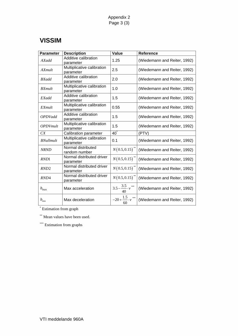
The model is in similar fashion as the Fritzsche model constituted by thresholds that form regimes. Figure 4 displays the thresholds and regimes in the relative speed relative position space. The threshold definitions presented in this paper, are taken from Wiedemann and Reiter (1992). The developer of VISSIM, PTV, refers to Wiedemann and Reiter (1992) for a complete listening of the random numbers used in the model. The exact difference between the car-following models used in VISSIM and Wiedemann and Reiter (1992) is not publicly known.


Figure 4 The different thresholds and regimes in the Wiedemann car-following model. • The desired distance between stationary vehicles, AX. This threshold consists

of the length of the front vehicle and the desired front-to-rear distance and is defined as

1 1n nAX L AXadd RND AXmult−= + + ⋅ ,

where and are calibration parameters. AXadd AXmult 1nRND is a normally distributed driver dependent parameter.

• The desired minimum following distance at low speed differences, ABX. This

threshold is calculated as

ABX AX BX= + with ( )1nBX BXadd BXmult RND v= + ⋅ ⋅ ,

where BXadd and BXmult are calibration parameters. The speed is defined as

v

1 1

1

for for

n n n

n nn

v v vv

v vv− −

−

>⎧= ⎨ ≤⎩

.

Upper limit of reaction

Free driving Closing in

SDV

SDX

Following CLDV OPDV

ABX

Emergency regime AX

0 v∆

x∆


• The maximum following distance, SDX. This distance varies between 1.5 and 2.5 times the minimum following distance, ABX, (PTV). SDX is defined as

SDX AX EX BX= + ⋅ with

( )2nEX EXadd EXmult NRND RND= + ⋅ − ,

where EXadd and EXmult are calibration parameters. is a normally distributed random number and

NRND2nRND is a normally distributed driver

dependent parameter • Approaching point, SDV. This threshold is used to describe the point where the

driver notices that he or she approaches a slower vehicle. SDV is defined as

21nx L AXSDV

CX−∆ − −⎛ ⎞= ⎜ ⎟

⎝ ⎠ with

( )( )1 2n nCX CXconst CXadd CXmult RND RND= ⋅ + ⋅ + ,

where , and CXm are calibration parameters. CXconst CXadd ult • Decreasing speed difference, CLDV. Wiedemann and Reiter (1992) includes

another threshold similar to SDV, to model perception of small speed differences at short, decreasing distances. In VISSIM this threshold is ignored and CLDV is simply assumed to be equal to SDV, (PTV).

• Increasing speed difference, OPDV. This threshold describes the point where

the driver observes that he or she is traveling at a lower speed than the leader. This threshold is defined as

( )OPDV CLDV OPDVadd OPDVmult NRND= ⋅ − − ⋅ ,

where and OPDVmult are calibration parameters. is a normally distributed random number.

OPDVadd NRND

The thresholds above give rise to the following car-following regimes: Following: The thresholds SDV, SDX, OPDV and ABX constitute the following regime. In order to account for inexact handling of the throttle, vehicles acceleration rate is assumed to always be separated from zero at all times. When a vehicle passes into the following regime, passing either the SDV or the ABX threshold it is assigned the acceleration rate –bnull and when passing the thresholds OPDV or SDX it is assigned the acceleration bnull.


The acceleration or deceleration rate, bnull, is defined as

( )4null nb BNULLmult RND NRND= ⋅ + ,

where BNULLmult is a calibration parameter. 4nRND is a normally distributed driver parameter and is a normally distributed random number. NRND Free driving: The vehicle is located above all thresholds in the phase diagram, Figure 4, and travels uninfluenced of the surrounding traffic. The vehicle uses its maximum acceleration to reach its desired speed. When the desired speed is reached, inexact handling of the throttle is modeled by assigning an acceleration of –bnull or bnull to the vehicle. The maximum acceleration, , for passenger cars is defined as maxb

( )max maxb BMAXmult v v FaktorV= ⋅ − ⋅ with

( )max

maxdes des

vFaktorVv FAKTORVmult v v

=+ ⋅ −

,

where is the vehicles maximum speed. is a calibration parameter.

maxv FAKTORVmult

Closing in: When passing the SDV threshold, the driver notices that he or she is approaching a slower vehicle. The driver decelerates in order to avoid collisions. The following deceleration rate is used:

( )2

11

12 ( )n n

n

vb b

ABX x L −−

∆= ⋅ +

− ∆ −,

where is the deceleration of the leader. 1nb −

Emergency regime: When the front to rear distance is smaller than ABX the follower adopt, if necessary, the following deceleration to avoid collision with the vehicle in front:

( )21

1 min1

( )12 ( )

nn n

n

v ABX x Lb b bAX x L BX

−−

−

∆ − ∆ −= ⋅ + + ⋅

− ∆ −

The vehicle’s maximum deceleration rate, , is calculated as minb

min 3n nb BMINadd BMINmult RND BMINmult v= − − ⋅ + ⋅ ,

where BMINadd and BMINmult are calibration parameters. 3nRND is a normally distributed driver parameter.


4 Comparison of car-following models In order to enlighten and compare the car-following behavior of the four simulation software packages a numerical experiment has been carried out. This section described the experiment and the outcome of it. The section also includes a discussion of the general structure and complexity of the models. This discussion is founded on the above presented formulae. The main objective of this comparison is to compare reaction magnitudes and reaction times of the four models. 4.1 Test The car-following equations of the four models AIMSUN, MITSIM, Fritzsche (Paramics) and VISSIM as presented in section 3 have been implemented in MATLAB. The used model parameter values are given in appendix 2. Each model’s follower equation has then been allowed to act on the same driving course of events of an artificial leader. The outcome of the experiment is then for all four models the follower’s driving course of events when constrained by the same leader.

The following driving course of events of the leader – follower pair was imple-mented: The leader started to drive with constant speed, 20 m/s, the follower was given a front to rear distance of 28 m to the leader and the same initial speed as the leader. After 40 s, the leader started to decelerate with a rate of 2 m/s2. The deceleration lasted for 2 s. After an additional time of 18 s, the leader started to accelerate with a rate of 2 m/s2. In similar fashion as the previous deceleration; the acceleration lasted for 2 s. Both the deceleration and acceleration of the leader was implemented as simple steps, that is, in the time step before the action the leader’s acceleration rate was zero and in the next time step the acceleration rate was immediately changed to 2 m/s2.

The resulting trajectories for each of the four models are displayed in Figure 5–Figure 8 below. Figure 5 shows the safety distance nature of the Gipps/AIMSUN car-following model. As can be seen in the figure, a front to rear distance of ~24 m was desired, when traveling at 20 m/s. At first the distance between the vehicles is 28 m and the follower adjusts its speed in order to reach the desired distance. As seen in the figure the follower reaches the desired distance after about 16 seconds. The follower’s non-smooth acceleration trajectory is caused by the discrete action change of AIMSUN’s model. The follower changes its speed at points in time separated by one reaction time. The figures also show that the following part of the AIMSUN model is almost symmetric regarding acceleration and deceleration behavior.


Figure 5 Speed, acceleration and distance gap for the AIMSUN car-following model. MITSIM’s reaction to the experiment is shown in Figure 6. Notice the asymmetric behavior for acceleration and deceleration.


Figure 6 Speed, acceleration and distance gap for the MITSIM car-following model. The MITSIM trajectories indicate that the smooth response of the follower to the leader’s deceleration in the car-following regime makes it necessary for the follower to use the emergency regime in order to achieve the desired following distance. In similar fashion when responding to the leader’s acceleration the follower is not able to respond without entering the free regime and using its maximum acceleration rate.

The Paramics model’s behavior, controlled by the Fritzsche model, is shown in Figure 7. The follower is assumed to have caught its leader and therefore employ a negative deceleration rate at t = 0. The effects of the closing in and free driving regimes are visualized though the spikes of the acceleration trajectory. In these regimes the follower uses a constant acceleration or deceleration rate in order to decrease or increase the distance to its leader.


Figure 7 Speed, acceleration and distance gap for the Fritzsche (Paramics) car-following model.

Figure 8 displays VISSIM’s reactions to the leader’s action. The effect of the various regimes of the Wiedemann model is enlightened by the apparent unstableness in the acceleration curve. Notice that the reaction is much larger when the vehicle passes out in to the free driving regime compared to when it is getting too close to the leader. Ignoring the speed oscillations at steady state the follower reacts almost exactly as the leader.


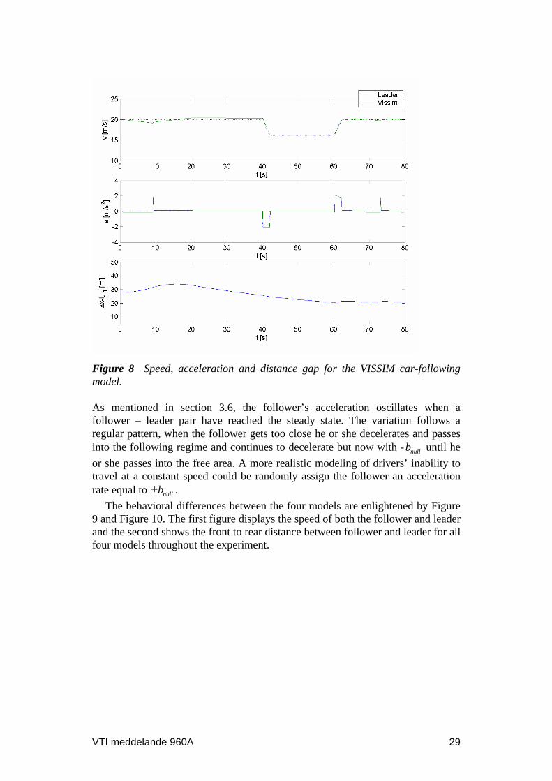
Figure 8 Speed, acceleration and distance gap for the VISSIM car-following model. As mentioned in section 3.6, the follower’s acceleration oscillates when a follower – leader pair have reached the steady state. The variation follows a regular pattern, when the follower gets too close he or she decelerates and passes into the following regime and continues to decelerate but now with - until he or she passes into the free area. A more realistic modeling of drivers’ inability to travel at a constant speed could be randomly assign the follower an acceleration rate equal to .

nullb

nullb±The behavioral differences between the four models are enlightened by Figure

9 and Figure 10. The first figure displays the speed of both the follower and leader and the second shows the front to rear distance between follower and leader for all four models throughout the experiment.


Figure 9 Speed of follower and leader during the driving course of events.

Figure 10 Front to rear distance between follower and leader during the driving course of events.


VISSIM and Fritzsche model inexact throttle control by applying a small acceleration or deceleration rate to the follower at every time step in the following regime. This has one side effect; the follower switches regimes even if the leader drives at constant speed, i.e. the follower changes its behavior without any action from the leader. This is the reason behind the oscillations of the follower trajectories in Figure 7 and Figure 8. Oscillations of this kind are however found among real drivers, (Leutzbach, 1988). VISSIM’s and Paramics’s approach might make the resulting microscopic driving course of events more close to those observed in real traffic but the impact on macroscopic traffic measures such as average speed and flow is not fully investigated.

AIMSUN uses a driver reaction time equal to the simulation time step, thus drivers react to leader actions immediately in the next time step. The reaction time is also equal for all drivers. MITSIM assigns an individual reaction time to every vehicle. When traveling in the car-following regime, vehicles acceleration is updated with the frequency of their assigned reaction times. VISSIM and Paramics do not model driver reaction time explicitly. Instead the reaction time is modeled as the time it takes for the follower to for example leave the following regime and enter the closing in regime. See section 3.2 for the discussion on how the reaction time influences the result. Ideally, in order to produce correct microscopic output, an individual reaction time for each driver drawn from a suitable distribution should be strived for.

In the AIMSUN and VISSIM models the follower’s reaction is of the same magnitude as the leader’s preceding action. MITSIM’s follower reaction is smaller than the preceding action of the leader. The MITSIM model is therefore slower in restoring, for example, the front to rear distance between follower and leader. Smaller follower reactions than leader actions are probably more realistic, since reactions should be damped throughout vehicle platoons to avoid asymptotic unstableness and produce travel times corresponding to real traffic.

The VISSIM and Paramics models use a small random acceleration or deceleration even without any change in leader behavior. This results in frequent changes in the sign of the follower’s acceleration. This may reflect real driving behavior, but it is likely to increase the calibration and validation work. 4.2 Discussion Traffic micro-simulation models typically use a large number of parameters such as desired speed, safety distances, perception thresholds and so forth. All of these parameters must be calibrated in order to create reliable simulation output. The calibration work increases very fast with the total number of parameters. It is therefore desirable to use models that produce representative driving trajectories using as few calibration parameters as possible.

Models with a large number of parameters increase the model makers’ role in the calibration work. It becomes important with good default values on the calibration parameters.

Among the studied models, VSSIM is the one with the largest number of parameters. VISSIM’s parameters are also not easily interpreted to known driving factors such as, for example, desired speed. These two factors have a significant potential to increase the necessary calibration work. The developer has solved this by letting the user set calibration parameter values by specifying the parameter distribution directly through its graph. The same holds for the Fritzsche model of


Paramics, which is similar to VISSIM’s Wiedemann model and contains about the same number of parameters.

AIMSUN is probably the model with the smallest number of parameters and the most intuitive parameter definitions. This allows for relatively little calibration work to be necessary in order to achieve the best possible results the model can produce. The question in AIMSUN’s case is if there are enough parameters to reflect driver behavior good enough. Many degrees of freedom in the car-following model are an absolute necessity if the model is to be utilized for different traffic situations. Remember it may not even be enough with one common car-following model for all traffic situations.

The number of parameters used in MITSIM is relatively small. The utilized parameters are however not easily interpreted to known driver or vehicle factors and may therefore be hard to calibrate. The GHR-model of MITSIM nevertheless incorporates many degrees of freedom and should therefore be possible to use for many different traffic situations.

All models have parameters that affect the reaction magnitude. As mentioned in section 3.2, the reaction magnitude influences the average speed, flow and density. It is therefore important that the reaction magnitude can be tuned, in order to achieve good agreement at the macro level.

In MITSIM, the reaction magnitude is calibrated with the model parameters of the GHR model, i.e. ,α β± ± and γ ± . These parameters offer good possibilities to calibrate the car-following model. The α -parameter affects the reaction magni-tude directly while β and γ mostly influences the behavior, but indirectly they also affect the reaction magnitude.

In AIMSUN, the reaction magnitude increases with increased difference between the estimation of the leader’s deceleration and the normal deceleration rate desired by the follower. The reaction magnitude also increases with decreasing desired normal deceleration rate, which may seem contradictory. Moreover, in AIMSUN, the desired distance between two vehicles in the following regime depend on the follower’s and the leader’s maximum desired deceleration, their speeds and the reaction time of the follower. Given that their speeds are equal, that is , which holds when the desired following distance is achieved, the desired space headway can be expressed as (notation as in section 3.3):

1n nv v −= = v

( )( )( )

1 1 1

1

1

ˆ ˆ ˆ21ˆ2

n n n n n n

n

n n

d d v d d d d Tx v s

d d

− − −

−

−

⋅ + ⋅ − + ⋅ ⋅∆ = ⋅ ⋅ +

⋅

When the deceleration ability of the leader is equal to the follower’s, the desired distance increases linearly with the speed of the vehicles. In the case when the follower estimates the leader’s desired deceleration rate as larger than its own, the desired headway is proportional to the square of the speed. Both these cases are plausible. However, if the follower estimates its own desired deceleration rate as larger than the leader’s, the relationship between the desired distance and the speed becomes proportional to -v2. This implies that that the desired distance decreases with speed at high speeds. Gipps following model is based upon the assertion that the follower should always be able to react to the leader’s action to


avoid collisions. Given that the follower’s maximum deceleration rate is larger than the leader’s, it is clear that the follower can answer any leader action when traveling with at gap to the leader corresponding only to the follower’s reaction time. This behavior is not very realistic. The follower’s estimation of the leader’s deceleration rate should, according to our opinion, never be smaller than the follower’s own maximum deceleration rate. A solution to this problem may be to use a minimum desired time gap between vehicles.

VISSIM offers several calibration parameters for calibrating the reaction magnitude. The parameter can be used to calibrate the speed oscillation in the following regime. The acceleration and deceleration magnitude can be adjusted through the parameters and , respectively. In the “closing in” and “emergency” regime, the deceleration also depends on the thresholds SDV, SDX CLDV, ABX and AX. These thresholds therefore affect the reaction magnitude indirectly.

nullb

minb maxb


5 Conclusions We have in this work described and compared the car-following models utilized in four traffic micro-simulation software packages. A general presentation of car-following models and desirable properties of such models has also been given. The requirements of a car-following model vary. When microscopic outputs are needed, the model must be able to describe the following behavior in detail. Whereas, if macroscopic results is needed, a more generalized approach can be used. Regardless of the level of detail a car-following model must offer the possibility to calibrate the reaction time and the reaction magnitude.

AIMSUN, MITSIM, and Fritzsche/VISSIM have relatively different presentation of their car-following models. The parameter choice is significantly different. The resulting car-following trajectories of a follower – leader vehicle pair are, in some cases, nevertheless similar. AIMSUN show a follower behavior that is very close to the behavior of the leader. The same holds for VISSIM and Paramics when reacting to the leader’s deceleration and acceleration, but not at steady state following. MITSIM’s follower reaction is smoother than the leader’s action but not powerful enough, which leads to for example emergency decelerations. In real traffic the follower reactions is normally damped throughout vehicle platoons. Smoother response than stimuli should therefore be preferable.

The robustness and stability of a car-following model depend strongly on the model parameters. The difficulty of calibrating the model increases fast with the number of parameters to be calibrated. We therefore believe that it is desirable to keep the number of parameters as low as possible. However, as discussed in section 3.2 the parameterization used must allow for the model to be well calibrated with respect to all proposed applications.

All four studied programs use a very coarse approach to the modeling of driver’s reaction time. A simple way of improving the reaction time modeling would be to assign individual reaction times to drivers, drawn from some suitable distribution, and let the individual driver’s reactions be delayed accordingly.

Further research is needed to achieve complete insight in the state of the art in elementary models used in traffic simulation. This paper should nevertheless be useful to anyone interested in the underlying models of the frequently used micro-simulation software packages. A more solid comparison of car-following would require driving course of events that represent real traffic better than the simple stepwise acceleration used in this study, the most preferable would of course be data from a real traffic system.

Interesting next steps on the path outlined by this study would be to investigate how follower reactions propagate through a platoon of vehicles.


6 References Al-Shihabi, T. and Mourant, R.R. (2003). Toward More Realistic Driving

Behavior Models for Autonomous Vehicles in Driving Simulators. 82nd Annual Meeting of the Transportation Research Board, Washington, D. C.

Bloomberg, L., Swenson, M. and Haldors, B. (2003). Comparison of Simulation Models and the HCM. TRB, Transportation Research Board, Washington D.C.

Brackstone, M. and McDonald, M. (1998). "Car-following: a historical review." Transportation Research F 2: 181–196.

Brockfeld, E., Kühne, R.D., Skabardonis, A. and Wagner, P. (2003). Towards a benchmarking of microscopic traffic flow models. TRB, Transportation Research Board, Washington D.C.

Fritzsche, H-T. (1994). "A model for traffic simulation." Transportation Engininering Contribution 5: 317–321.

Gipps, P.G. (1981). "A behavioural car-following model for computer simulation." Transportation Research B 15: 105–111.

Hoogendoorn, S.P. and Bovy, P.H.L. State-of-the-art of Vehicular Traffic Flow Modelling. http://www.trail.tudelft.nl/T&E/papers_course_IV_9/state-of-the-art.PDF, accessed Jul. 17, 2003.

ITS University of Leeds (2000). SMARTEST – Final report for publication, University of Leeds.

Leutzbach, W. (1988). Introduction to the theory of traffic flow. Berlin, Springer Verlag.

May, A.D. (1990). Traffic Flow Fundamentals. Upper Saddle River, Prentice Hall.

MIT, MITSIM. http://web.mit.edu/its/papers/MITSIM2001.pdf, accessed Jun. 16, 2003.

PTV VISSIM Traffic flow simulation – Technical Description, PTV Planung Transport Verkehr AG.

PTV, VISSIM. http://www.english.ptv.de/cgi-bin/produkte/vissim.pl, accessed Jun. 16, 2003.

Quadstone, Quadstone Paramics. http://www.paramics-online.com, accessed Jun. 16, 2003.

Saldaña, R.P. and Tabares, W.C. (2000). Traffic Modeling on High Perfor-mance Computing Systems. Philippine Computing Science Congress (PCSC).

SIAS, SIAS Paramics. http://www.sias.com/sias/homepage.html, accessed Jun. 16, 2003.

Transportation Research Board (1997). Highway Capacity Manual. Washington DC.

TSS (2002). AIMSUN version 4.1 User Manual, Transport Simulation Systems. TSS, AIMSUN. http://www.aimsun.com/brochure.pdf, accessed Jun. 16, 2003. Wiedemann, R. (1974). Simulation des Strassenverkehrsflusses (in German),

University Karlsruhe. Wiedemann, R. and Reiter, U. (1992). Microscopic traffic simulation: the

simulation system MISSION, background and actual state. Project ICARUS (V1052) Final Report. Brussels, CEC. 2: Appendix A.

Yang, Q. (1997). A Simulation Laboratory for Evaluation of Dynamic Traffic Management Systems. Department of Civil and Environmental Engineering, Massachusetts Institute of Technology: 193.


http://www.trail.tudelft.nl/T&E/papers_course_IV_9/state-of-the-art.PDF

http://www.trail.tudelft.nl/T&E/papers_course_IV_9/state-of-the-art.PDF

http://web.mit.edu/its/papers/MITSIM2001.pdf

http://www.english.ptv.de/cgi-bin/produkte/vissim.pl

http://www.paramics-online.com/

http://www.sias.com/sias/homepage.html

http://www.aimsun.com/brochure.pdf

Yang, Q. and Koutsopoulos, H.N. (1996). "A microscopic traffic simulator for evaluation of dynamic traffic management systems." Transportation Research C 4: 113–129.


Appendix 1 Page 1 (2)

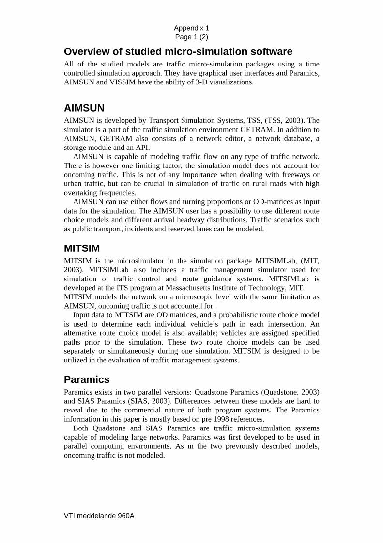
Overview of studied micro-simulation software All of the studied models are traffic micro-simulation packages using a time controlled simulation approach. They have graphical user interfaces and Paramics, AIMSUN and VISSIM have the ability of 3-D visualizations.

AIMSUN AIMSUN is developed by Transport Simulation Systems, TSS, (TSS, 2003). The simulator is a part of the traffic simulation environment GETRAM. In addition to AIMSUN, GETRAM also consists of a network editor, a network database, a storage module and an API.

AIMSUN is capable of modeling traffic flow on any type of traffic network. There is however one limiting factor; the simulation model does not account for oncoming traffic. This is not of any importance when dealing with freeways or urban traffic, but can be crucial in simulation of traffic on rural roads with high overtaking frequencies.

AIMSUN can use either flows and turning proportions or OD-matrices as input data for the simulation. The AIMSUN user has a possibility to use different route choice models and different arrival headway distributions. Traffic scenarios such as public transport, incidents and reserved lanes can be modeled.

MITSIM MITSIM is the microsimulator in the simulation package MITSIMLab, (MIT, 2003). MITSIMLab also includes a traffic management simulator used for simulation of traffic control and route guidance systems. MITSIMLab is developed at the ITS program at Massachusetts Institute of Technology, MIT. MITSIM models the network on a microscopic level with the same limitation as AIMSUN, oncoming traffic is not accounted for.

Input data to MITSIM are OD matrices, and a probabilistic route choice model is used to determine each individual vehicle’s path in each intersection. An alternative route choice model is also available; vehicles are assigned specified paths prior to the simulation. These two route choice models can be used separately or simultaneously during one simulation. MITSIM is designed to be utilized in the evaluation of traffic management systems.

Paramics Paramics exists in two parallel versions; Quadstone Paramics (Quadstone, 2003) and SIAS Paramics (SIAS, 2003). Differences between these models are hard to reveal due to the commercial nature of both program systems. The Paramics information in this paper is mostly based on pre 1998 references.

Both Quadstone and SIAS Paramics are traffic micro-simulation systems capable of modeling large networks. Paramics was first developed to be used in parallel computing environments. As in the two previously described models, oncoming traffic is not modeled.

VTI meddelande 960A


VISSIM VISSIM is developed by Planung Transport Verkehr, PTV, (PTV, 2003). The system consists of two separate parts; the traffic simulator and the signal state generator. PTV frequently accentuates simulation of vehicle-actuated signal controls as a typical application of the VISSIM model.

VISSIM models urban and motorway traffic that is roads without oncoming traffic. VISSIM has similar modeling capabilities as the previously described program systems.

VTI meddelande 960A


Simulation parameters

All models Parameter Description Value

1nL − Length, vehicle n-1 4.5 m desirednv Desired speed, vehicle n 40 m/s

AIMSUN Parameter Description Value

minx∆ Min distance between stationary vehicles 1 m

maxna Maximum acceleration,

vehicle n 2.5 m/s2

maxnd Maximal desired

deceleration, vehicle n 2 m/s2

T Reaction time 0.7 s

MITSIM Parameter Description Speed [m/s] Reference < 6.1 6.1–12.2 12.2–18.3 18.3–24.4 > 24.2

na− Normal deceleration rate, vehicle n

8.7 m/s2 5.2 m/s2 4.4 m/s2 2.9 m/s2 2 m/s2 (Yang, 1997)

Parameter Description Speed [m/s] Reference 6.096< 6.096 12.192− 12.192>

na + Maximum acceleration rate, vehicle n

7.8 m/s2 6.7 m/s2 4.8 m/s2 (Yang, 1997)

Parameter Description Value Reference

α+ Car-following parameter, acceleration 2.15 (Yang, 1997)

β + Car-following parameter, acceleration -1.67 (Yang, 1997)

γ + Car-following parameter, acceleration -0.89 (Yang, 1997)

α− Car-following parameter, deceleration 1.55 (Yang, 1997)

β − Car-following parameter, deceleration 1.08 (Yang, 1997)

γ − Car-following parameter, deceleration 1.65 (Yang, 1997)

upperh Max following time headway 1.36 s (Yang, 1997)

lowerh Min following time headway 0.5 s (Yang, 1997)

VTI meddelande 960A


Fritzsche (Paramics) Parameter Description Value Reference

1ns − Effective length, vehicle n-1 6 m (Fritzsche, 1994)

DT Desired time gap 1.8 s (Fritzsche, 1994)

rT Risky time gap 0.5 s (Fritzsche, 1994)

sT Safe time gap 1 s (Fritzsche, 1994)

mb∆ Deceleration parameter 0.4 m/s2 * (Fritzsche, 1994)

xf Calibration parameter 0.5* (Fritzsche, 1994)

PTPk Calibration parameter 0.001* (Fritzsche, 1994)

PTNk Calibration parameter 0.002* (Fritzsche, 1994)

nullb Acceleration parameter 0.2 m/s2 (Fritzsche, 1994)

na+ Normal acceleration rate 2 m/s2 (Fritzsche, 1994)

* Estimation from graph

VTI meddelande 960A


VISSIM Parameter Description Value Reference

AXadd Additive calibration parameter 1.25 (Wiedemann and Reiter, 1992)

AXmult Multiplicative calibration parameter 2.5 (Wiedemann and Reiter, 1992)

BXadd Additive calibration parameter 2.0 (Wiedemann and Reiter, 1992)

BXmult Multiplicative calibration parameter 1.0 (Wiedemann and Reiter, 1992)

EXadd Additive calibration parameter 1.5 (Wiedemann and Reiter, 1992)

EXmult Multiplicative calibration parameter 0.55 (Wiedemann and Reiter, 1992)

OPDVadd Additive calibration parameter 1.5 (Wiedemann and Reiter, 1992)

OPDVmult Multiplicative calibration parameter 1.5 (Wiedemann and Reiter, 1992)

CX Calibration parameter 40* (PTV)

BNullmult Multiplicative calibration parameter 0.1 (Wiedemann and Reiter, 1992)

NRND Normal distributed random number ( )0.5,0.15N ** (Wiedemann and Reiter, 1992)

1RND Normal distributed driver parameter ( )0.5,0.15N ** (Wiedemann and Reiter, 1992)



maxb Max acceleration 3.53.540

v− ⋅ *** (Wiedemann and Reiter, 1992)

minb Max deceleration 1.52060

v− + ⋅ *** (Wiedemann and Reiter, 1992)

* Estimation from graph ** Mean values have been used. *** Estimation from graphs

VTI meddelande 960A

johan janson olstam andreas tapani - diva portal673977/fulltext01.pdf · johan janson olstam och...

Documents