joint discussion paper series in economics - uni … · 28magks%29 ... row pearson spearman pearson...

Joint Discussion Paper

Series in Economics

by the Universities of

Aachen ∙ Gießen ∙ Göttingen Kassel ∙ Marburg ∙ Siegen

ISSN 1867-3678

No. 33-2013

Christian Westphal

Evidence for the “Suicide by Firearm” Proxy for Gun Ownership from Austria

This paper can be downloaded from http://www.uni-marburg.de/fb02/makro/forschung/magkspapers/index_html%28magks%29

Coordination: Bernd Hayo • Philipps-University Marburg Faculty of Business Administration and Economics • Universitätsstraße 24, D-35032 Marburg

Tel: +49-6421-2823091, Fax: +49-6421-2823088, e-mail: [email protected]

mailto:[email protected]

Evidence for the “Suicide by Firearm” Proxy

for Gun Ownership from Austriaa

Christian Westphalb

This version: July 10, 2013

Abstract

When attempting to measure gun ownership in the United States, the

problem of missing administrative data arises, making it necessary to find a

valid proxy. Several such proxies are employed in economic studies, one of

which is the fraction of “suicides by firearm” of “all suicides” (FSS). My work

validates this proxy from out-of-sample data, namely, Austrian administra-

tive data on firearm licenses. I also reevaluate, with appropriate statistical

methods, a result on firearms and suicide from the medical that is often used

for public policy advocacy. This result is, unfortunately, heavily biased due

to ignoring a well-known fallacy and thus can be only partially confirmed.

JEL Classifications: C15; C51; I18

Keywords: Gun Ownership; Suicide; Ratio Fallacy; Spurious Correlation

aThanks to Matthew Lang for sharing his data on suicide and firearms in the United Stateswith me, which allowed me to perfectly replicate his findings.

bUniversity of Marburg, Faculty of Business Administration and Economics, Department of

Statistics, westphal�staff.uni-marburg.de, hristian.westphal�westphal.dei

1 INTRODUCTION 11 Introdu tionThe economic literature contains ample investigation into the relation between

guns and crime. Seeing that in the United States there were 11,078 deadly as-

saults by firearm and 19,392 suicides by firearm in 2010,1 a closer investigation

of a possible association between firearms and suicide seems warranted. Two

studies of Ireland (Kennelly, 2007; Yang and Lester, 2007) – with remarkably

different outcomes – elaborate on the economic dimension of suicide in terms

of cost. Furthermore, firearm suicide as a fraction of all suicides is believed to

be a good proxy, at least in the cross-section, for gun ownership density (Azrael,

Cook and Miller, 2004; Kleck, 2004). This association is exploited by Cook and

Ludwig (2006) in a very detailed, albeit flawed (Westphal, 2013), analysis of the

association between firearms and crime. Lang (2013) analyzes the association

between firearms and suicide using U.S. National Instant Background Check data

and confirms the validity of the FSS proxy.It seems valuable to investigate the in-

teraction between firearms and suicide with high quality data from other than a

U.S. sample, taking care to avoid methodological fallacies.

After World War II, European countries enacted much tighter firearms regu-

lation than what exists in the United States. Therefore, much better administra-

tive data are available. Austria has relatively low restrictions on the acquisition

of firearms but has become increasingly concerned with monitoring legally pur-

chased firearms. Austrian data on concealed carry licenses are available from

1982 to the present for all Austrian counties. This provides a reasonable, albeit

imperfect, nationwide proxy for gun ownership taken directly from administra-

tive data on firearm permits. These data have been used to compute correlations

between firearm ownership rates and suicide rates in the medical literature (Et-

zersdorfer, Kapusta and Sonneck, 2006), and provide an intriguing starting point

for possibly confirming, or not, the validity of the FSS proxy and at the same time

further investigating the relationship between suicide and firearms.

Two questions are addressed in this paper: (1) Can the FSS proxy for gun

ownership be confirmed from Austrian data on gun licenses? – and (2) What

can be said about the relationship between firearms and suicide in Austria after

a careful review of the methods used for analysis in former work? Answering

these questions results in two main findings. First, I confirm the validity of the

FSS proxy. An association between firearms and firearm suicides is persistent

across all methods of analysis used and a variety of model specifications. If one

prefers clustered standard errors over Driscoll-Kraay standard errors – a prefer-

ence I do not advocate in my setting – a substitution between suicide methods

1ICD-10 codes X93, X94, and X95 used for “assault by firearm”; X72, X73, and X74 for “suicide

by firearm.” Values taken from United States Department of Health and Human Services (2010).

2 FORMER ANALYSIS 2

shows in the main model. Second, it is clear that, earlier correlation results in

Etzersdorfer, Kapusta and Sonneck (2006) on the association between firearms

and suicides are greatly overstated due to ignoring Pearson’s (1896) finding on

spurious correlations between ratio variables. Thus, the contributions of this pa-

per include validation of earlier approaches to measuring gun ownership,2 and a

warning as to the hazards of using spurious results in public policy debate.

My paper is organised as follows. I revisit the literature on guns and suicide

in Austria in Section 2. In Section 3.1, the results from Etzersdorfer, Kapusta

and Sonneck (2006) are repeated. Sections 3.2 and 3.3 point out the statistical

fallacy in Etzersdorfer, Kapusta and Sonneck (2006) and adjust for the problem

using two approaches that both lead to numerically very close and qualitatively

identical results. Section 4 motivates and estimates a fixed effects panel model

based on a theoretical model from the economic literature. The main finding for

the FSS proxy is found to be robust to several robustness checks in Section 4.2.2 Former Analysis of Firearms and Sui ides inAutriaEtzersdorfer, Kapusta and Sonneck (2006) (EKS hereafter) analyze correlations

between suicide rates and rates of firearm ownership, proxied by the rate of con-

cealed carry licenses, in all nine Austrian counties over the period from 1990 to

2000. Their results from a repeated cross-sectional analysis are strong rank cor-

relations between the firearms measure and firearm suicides, low-to-no rank corre-

lations between firearms and other suicides, and weakly positive rank correlations

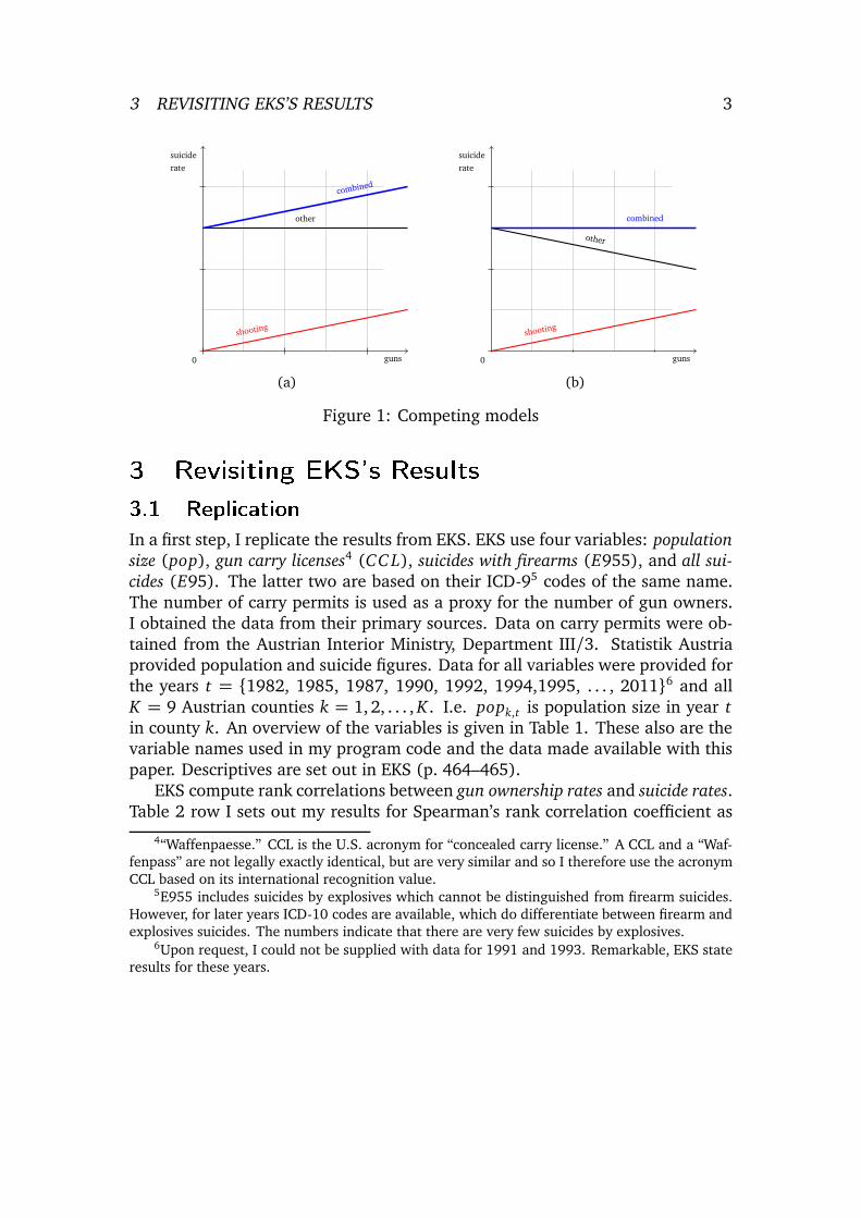
between firearms and all suicides. Based on these findings, their conclusion is to

assume that overall suicides increase with more firearms, as depicted in Figure

1(a), as opposed to a substitution between suicide methods as shown in Figure

1(b). In EKS’s (p. 468) opinion their findings “emphasise the need for political

support” for stricter regulation on gun ownership in the interest of preventing

suicide. Their finding is now propagated through the literature; for example, “it

is a scientific fact . . . that reducing the availability of guns . . . will reduce deaths”

(Leenaars, 2006, 439). There many references to similar studies3 can be found.

2This measure is not without problems itself as can be seen in Westphal (2013).3Notably similar to EKS of those mentioned are Markush and Bartolucci (1984), Killias (1993)

and Leenaars et al. (2003).

3 REVISITING EKS’S RESULTS 3

0 guns

suicide

rate

shooting

other

combined

(a)

0 guns

suicide

rate

shooting

other

combined

(b)

Figure 1: Competing models3 Revisiting EKS's Results3.1 Repli ationIn a first step, I replicate the results from EKS. EKS use four variables: population

size (pop), gun carry licenses4 (CC L), suicides with firearms (E955), and all sui-

cides (E95). The latter two are based on their ICD-95 codes of the same name.

The number of carry permits is used as a proxy for the number of gun owners.

I obtained the data from their primary sources. Data on carry permits were ob-

tained from the Austrian Interior Ministry, Department III/3. Statistik Austria

provided population and suicide figures. Data for all variables were provided for

the years t = {1982, 1985, 1987, 1990, 1992, 1994,1995, . . . , 2011}6 and all

K = 9 Austrian counties k = 1, 2, . . . , K. I.e. popk,t is population size in year t

in county k. An overview of the variables is given in Table 1. These also are the

variable names used in my program code and the data made available with this

paper. Descriptives are set out in EKS (p. 464–465).

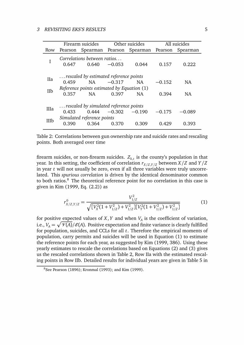
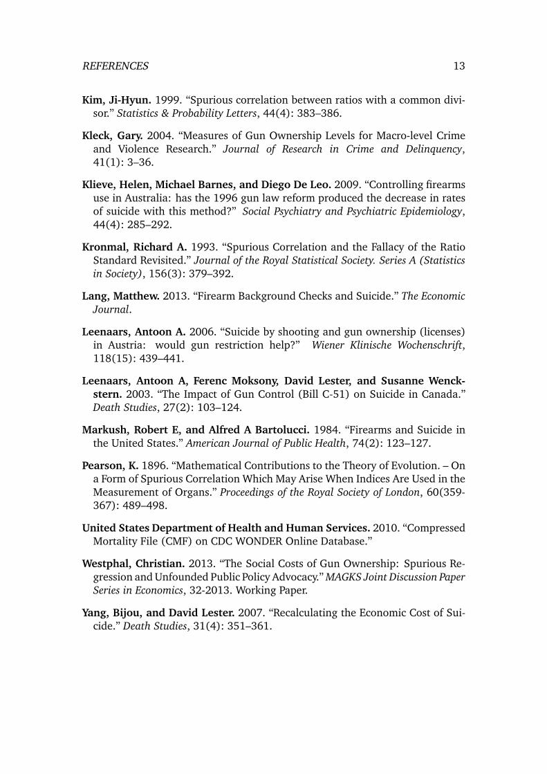
EKS compute rank correlations between gun ownership rates and suicide rates.

Table 2 row I sets out my results for Spearman’s rank correlation coefficient as

4“Waffenpaesse.” CCL is the U.S. acronym for “concealed carry license.” A CCL and a “Waf-fenpass” are not legally exactly identical, but are very similar and so I therefore use the acronym

CCL based on its international recognition value.5E955 includes suicides by explosives which cannot be distinguished from firearm suicides.

However, for later years ICD-10 codes are available, which do differentiate between firearm and

explosives suicides. The numbers indicate that there are very few suicides by explosives.6Upon request, I could not be supplied with data for 1991 and 1993. Remarkable, EKS state

results for these years.


Underlying Absolute Meaning Rate How computed?

Firearms CC LNumber of

CC LR C P/popcarry permits

FirearmE955

Number of fire-FSR E955/pop

suicides arm suicides

All suicides E95Number of

SR E95/popall suicides

Suicides notN E955

Number of suicidesOSR N E955/pop

with firearms not with firearms

Population popNumber of

NA NAinhabitants

Table 1: Variables and their meaning

well as Pearson’s correlation coefficient, averaged over all years t.7 Detailed

result for individual years can be found in Table 4 in the Appendix. Neither small

sample size nor non-normality of data, as claimed by EKS (p. 465), contradict

the computation of Pearson’s correlation coefficient. I therefore included these

values in Table 2: values do not deviate much from the rank correlations. Tables

2 and 4 reveal the numerical and qualitative results from EKS are robust to the

inclusion of years prior to and after their original period as well as to using either

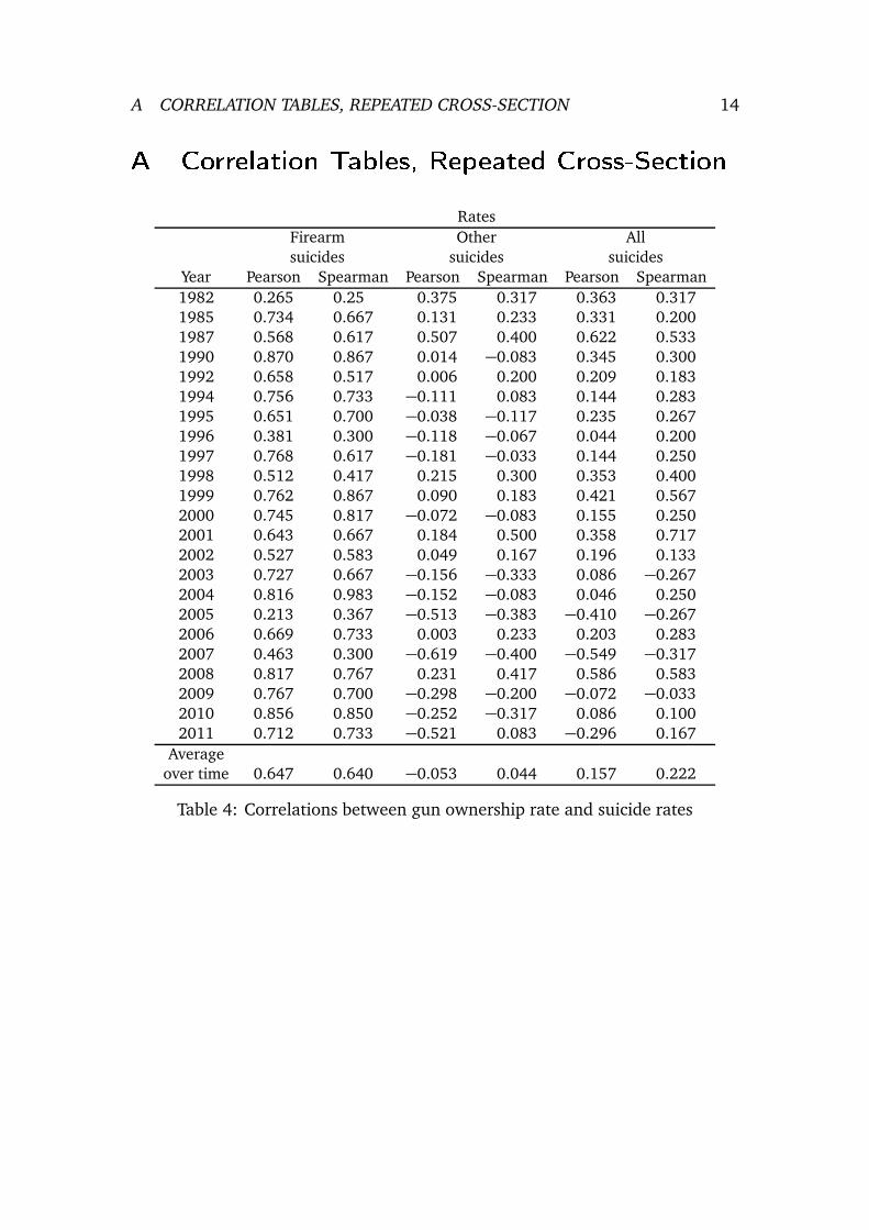
Pearson’s or Spearman’s method.3.2 A ounting for Spurious Correlation between RatiosUnfortunately, EKS fail to acknowledge Pearson’s finding on correlations between

ratios (Pearson, 1896): using ratios for correlation analysis may lead to spurious

results.

Table 2, Row I shows there is little difference between rank correlations and

Pearson’s correlation for the data. Because of this and because of the availabil-

ity of a theoretical result from Kim (1999), I now first use Pearson’s correlation

coefficient for illustration and examination of the ratio fallacy problem in EKS’s

results. A simulation study conducted in Section 3.3 shows that my findings do

not change when using rank correlations.

Let there be three independent random variables X , Y, Z with known expected

values and variances. To illustrate the problem at hand, let Xk,t be the number of

CCLs in county k in year t. Yk,t represents the corresponding number of suicides,

7As opposed to the rank correlation of the average rates over time (what is the meaning of thatvalue aside from it being larger than the individual correlations in this setting?) as in EKS (Table

2).


Firearm suicides Other suicides All suicides

Row Pearson Spearman Pearson Spearman Pearson Spearman

ICorrelations between ratios. . .

0.647 0.640 −0.053 0.044 0.157 0.222

IIa. . . rescaled by estimated reference points

0.459 NA −0.317 NA −0.152 NA

IIbReference points estimated by Equation (1)

0.357 NA 0.397 NA 0.394 NA

IIIa. . . rescaled by simulated reference points

0.433 0.444 −0.302 −0.190 −0.175 −0.089

IIIbSimulated reference points

0.390 0.364 0.370 0.309 0.429 0.393

Table 2: Correlations between gun ownership rate and suicide rates and rescaling

points. Both averaged over time

firearm suicides, or non-firearm suicides. Zk,t is the county’s population in that

year. In this setting, the coefficient of correlation rX/Z ,Y/Z between X/Z and Y /Zin year t will not usually be zero, even if all three variables were truly uncorre-

lated. This spurious correlation is driven by the identical denominator common

to both ratios.8 The theoretical reference point for no correlation in this case is

given in Kim (1999, Eq. (2.2)) as

r0X/Z ,Y/Z

=V 2

1/Zq

[V 2X(1+ V 2

1/Z) + V 2

1/Z][V 2

Y(1+ V 2

1/Z) + V 2

1/Z]

(1)

for positive expected values of X , Y and when VA is the coefficient of variation,

i.e., VA =p

V (A)/E (A). Positive expectation and finite variance is clearly fulfilled

for population, suicides, and CCLs for all t. Therefore the empirical moments of

population, carry permits and suicides will be used in Equation (1) to estimate

the reference points for each year, as suggested by Kim (1999, 386). Using these

yearly estimates to rescale the correlations based on Equations (2) and (3) gives

us the rescaled correlations shown in Table 2, Row IIa with the estimated rescal-

ing points in Row IIb. Detailed results for individual years are given in Table 5 in

8See Pearson (1896); Kronmal (1993); and Kim (1999).


the Appendix.

r∗X/Z ,Y/Z

=rX/Z ,Y/Z − r̂0

X/Z ,Y/Z

1+ r̂0X/Z ,Y/Z

∀rX/Z ,Y/Z ≤ r0X/Z ,Y/Z

(2)

r∗X/Z ,Y/Z

=rX/Z ,Y/Z − r̂0

X/Z ,Y/Z

1− r̂0X/Z ,Y/Z

∀rX/Z ,Y/Z > r0X/Z ,Y/Z

(3)

We obtain an average rescaled correlation of 0.46 between firearms and firearm

suicides. This is neither a very strong nor a very weak correlation. Thus associ-

ation between these two measures appears to persist after rescaling, albeit far

more weakly than stated by EKS. Between firearms and non-firearm suicides, the

average rescaled correlation over time takes a negative value of −0.32, which

is rather weak. What is remarkable is the change in sign compared to the spu-

rious results reported by EKS. Last, for all suicides, there is an average rescaled

correlation of −0.15. This is hard to interpret without testing for significance,

a problem addressed in Section 4. Without testing for significance, we have a

not very strong, but clearly present, positive correlation between the measure for

firearms and firearm suicides, a rather weak negative correlation between the

measure for firearms and other suicides, and a negative correlation between the

measure for firearms and all suicides too weak to base any findings on. However,

it is still clear that rejecting Model (b) of Figure 1 in favor of Model (a), as done

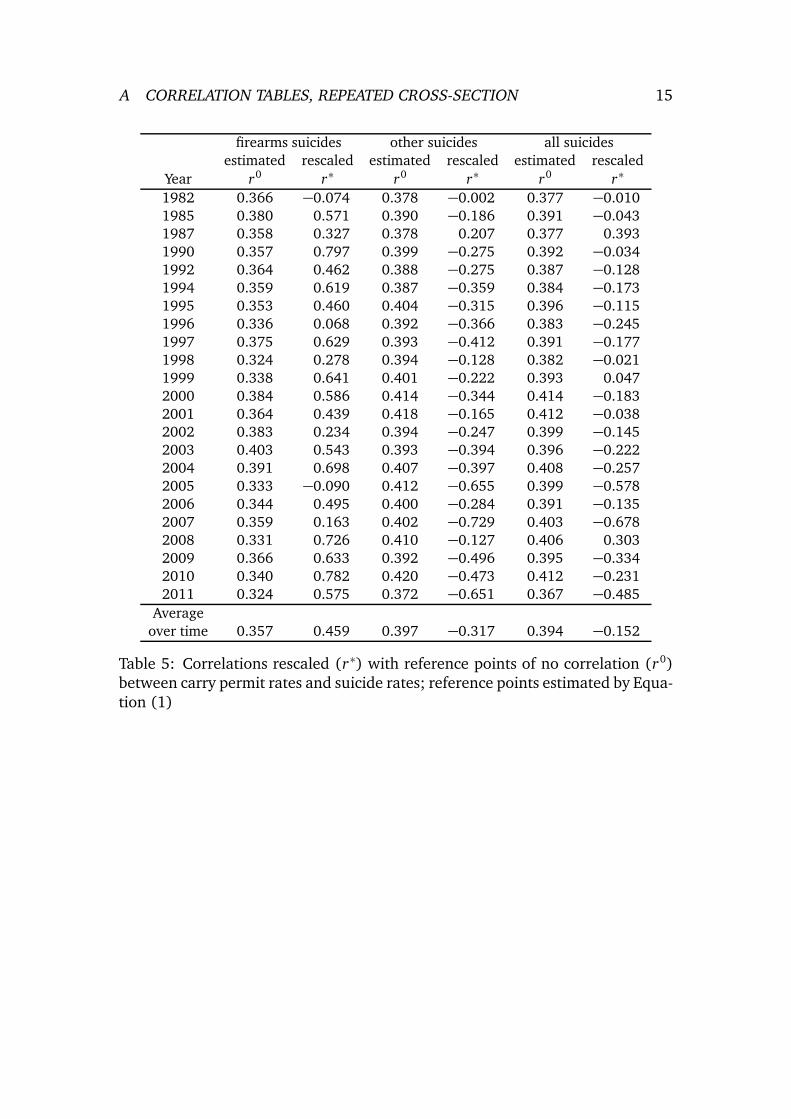
by EKS, is not advisable based on this empirical foundation.3.3 Simulation StudyThe results from Tables 2 (Rows IIa and IIb) and 5 while theoretically well founded

are surprising given how much they change the initial results. Also my results

report rescaled correlations for Pearson’s method and not for Spearman’s rank

correlation: ranks are not ratios. So, do the results hold for ranked ratios? Be-

cause I could find no theoretical result for spurious correlation reference points

for ranks of ratios, I conducted a simulation study.

I used a hotdeck simulation. For each year I repeatedly (10,000 times), ran-

domly, and independently redistributed the observed numerators (E95, E955,

CC L) across the counties, thus ensuring that, on average, there is no correlation

between the numerators. Fortunately, max{E95k,t , E955k,t , CC Lk,t}<min{popk,t}

∀t so no ratios > 1 could occur. I next, for each repetition, computed the same

ratios and ranks of ratios as done for the analysis in Sections 3.1 and 3.2. The

random rank correlations of the numerators generated in this manner appear to

be distributed around 0. (See Figure 2 in Appendix B for selected years.) The

ratios’ rank correlation distributions, on the other hand, are clearly shifted to

the right and obviously skewed (Appendix B, Figure 3). The situation is persis-

4 PANEL REGRESSION 7

tent for all years and Pearson’s correlations. The numerical results are well in

accordance with the correction derived from Kim’s (1999) theoretical result and

Pearson’s (1896) initial estimates of the problem size.

Year-wise simulated reference points can be calculated by computing the mean

of the simulated (rank) correlations between the ratios. These values then can be

used to rescale the results from the biased correlation analysis from Table 2, Row

I, resulting in Rows IIIa, IIIb, and the detailed Tables 6 and 7 for rank correlations

and Pearson’s correlations found in Appendix B.

Results from Table 2, Row IIIa and Tables 6 and 7 are intriguing: after rescal-

ing there remains, on average, a negative correlation between concealed carry

licenses and all suicides. Interpreting such low correlation coefficients in favor

of any side of any debate, however, is a tricky business. This question of valid

inference is addressed in Section 4 of this paper.4 Panel Regression4.1 Model and ResultsA more sophisticated method for analyzing the data seems appropriate. Panel

regression, in contrast to EKS’s repeated cross-sectional analysis, is capable of

accounting for the contemporal and intertemporal structure of the data. Panel

regression must be employed carefully as (a) either using ratios or (b) ignoring

time series effects may cause spurious results. (a) can be dealt with by consid-

ering a risk model, as outlined below; (b) is solved by estimating the model on

first differences.

The risk model is theoretically based on Duggan (2003).9 A binary choice

model is set up for individual i’s suicide decision in the form of a linear probability

model:

Pr(Suicidei) = α+ X iθ + γGuni +λi + ǫi. (4)

X i represents individual characteristics, Guni is a dummy indicating if i owns

a firearm, and the individual propensity λi tells us how strongly i is inclined

to commit suicide. As Duggan notes, if the unobservable λi and Guni are not

independent, we face a sample selection problem. Taking Duggan (2003, Eq. 2)

λi = µ+σGuni + ζi (5)

we see that unless σ = 0 in Equation (5), omitting λi introduces a bias into

estimation of Equation (4)’s parameters. This problem can be overcome by using

the data from above and imposing a risk model on the aggregate values. Let the

9I deviate slightly from Duggan’s notation without changing the model to keep my formulassimple.


number of suicides (all, firearm, or non-firearm) have a conditional expectation

of

E [Yk,t |X k,t , Gunk,t ,λk,t , popk,t] = popk,t (α+ X k,tθ + γGunk,t +λk,t) (6)

where X k,t ,λk,t are the averages of those values in county k in year t and Gunk,t

is the percentage of gun owners in k’s population in year t. When we assume the

average propensity and the average characteristics to be invariant over time, the

(averages of) controls in Xk,t and the propensities can be fully captured in a fixed

effect model’s county dummy. For those X i that are individual characteristics,

popX become the count of persons with these characteristics.

Slightly relaxing the restriction of time-invariant unobserved variables, iden-

tical intertemporal changes in X and λ across all Austria can be captured in a

time dummy. Then we arrive at a two-way fixed effects model of

yk,t = β0popk,t + β1CC Lk,t + dk + dt + ǫk,t . (7)

Here the number of concealed carry licenses is used as a proxy10 for the number of

gun owners. Then β0 can be interpreted identically to α from Equations (4) and

(6) as the baseline risk of an individual committing suicide. β1 will be related to γby the relation between concealed carry licenses and gun owners. A gun owner’s

relative risk of committing suicide from Equation (4), ignoring propensity for

illustrative purposes, will be related to the ratio of coefficients from Equation

(7):α+ X iθ + γ

α+ X iθ∼β0 + β1

β0

. (8)

Given the nature of the data, i.e., a panel with time series, to rule out spuri-

ous results from time series effects (which may be numerous), Equation (7) is

estimated on the first differences,11 i.e.,

∆yk,t = β0∆popk,t + β1∆CC Lk,t +δt + νk,t , (9)

which is a common technique for circumventing many time series problems. The

null hypothesis of poolability of the data, conducting a Chow test for poolability

across periods, is rejected for firearm suicides and all suicides as the dependent

variable with p-values12 < 0.05. Results are shown in Table 3. The association

10This will be a somewhat noisy proxy, of course, so we expect coefficient estimates to bebiased downward (Baltagi, 2008, Section 10.1).

11Including individual fixed growth parameters, i.e. a county dummy in the first differenced

model, leads to highly insignificant county fixed effects and to no qualitative change to the resultsset out in Tables 3 and 8.

12All standard errors are computed according to Driscoll and Kraay (1998); available for Stata

via xts from Hoechle (2007). Employing clustered robust standard errors does not qualita-tively change the results and – for all results reported to be significant on any level – uniformly

yields smaller p-values.


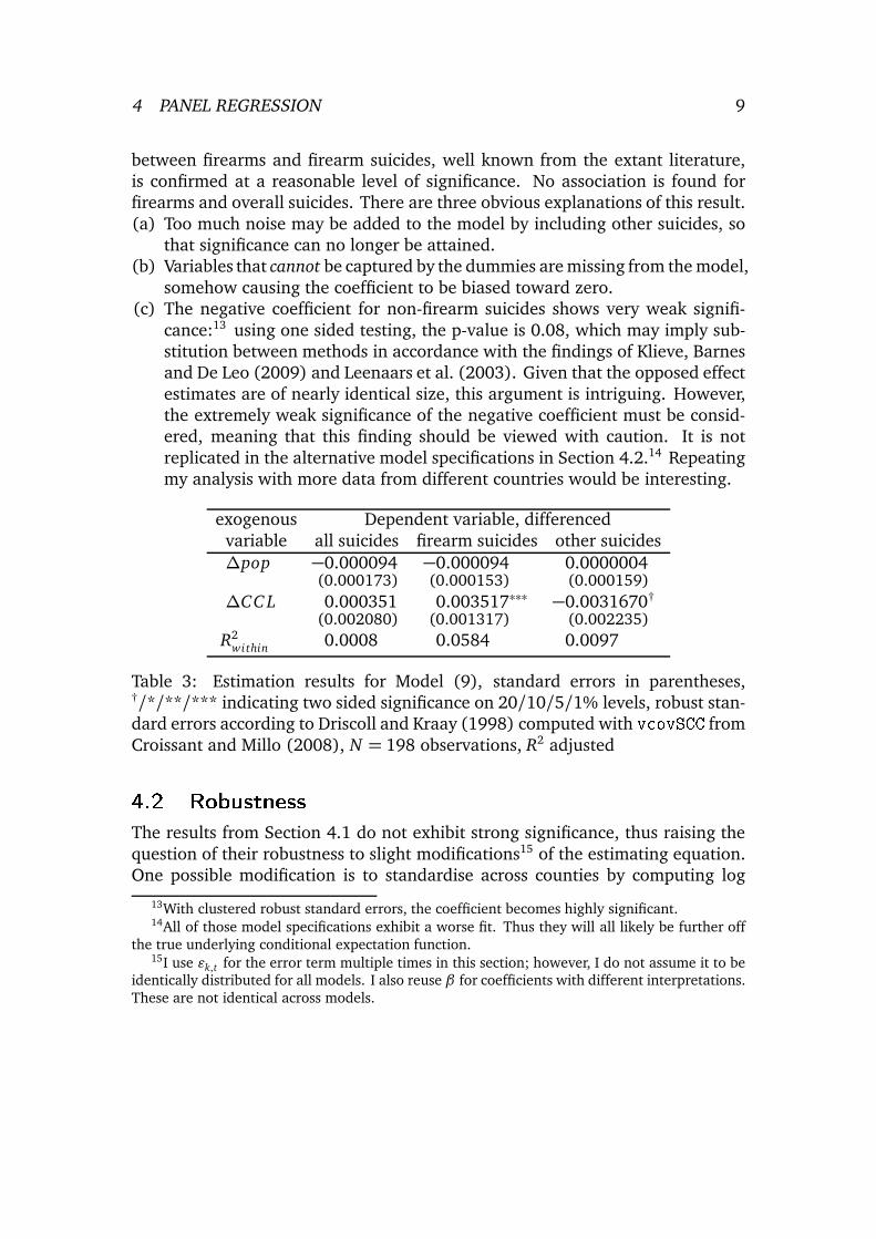
between firearms and firearm suicides, well known from the extant literature,

is confirmed at a reasonable level of significance. No association is found for

firearms and overall suicides. There are three obvious explanations of this result.

(a) Too much noise may be added to the model by including other suicides, so

that significance can no longer be attained.

(b) Variables that cannot be captured by the dummies are missing from the model,

somehow causing the coefficient to be biased toward zero.

(c) The negative coefficient for non-firearm suicides shows very weak signifi-

cance:13 using one sided testing, the p-value is 0.08, which may imply sub-

stitution between methods in accordance with the findings of Klieve, Barnes

and De Leo (2009) and Leenaars et al. (2003). Given that the opposed effect

estimates are of nearly identical size, this argument is intriguing. However,

the extremely weak significance of the negative coefficient must be consid-

ered, meaning that this finding should be viewed with caution. It is not

replicated in the alternative model specifications in Section 4.2.14 Repeating

my analysis with more data from different countries would be interesting.

exogenous Dependent variable, differenced

variable all suicides firearm suicides other suicides

∆pop −0.000094 −0.000094 0.0000004(0.000173) (0.000153) (0.000159)

∆CC L 0.000351 0.003517∗∗∗ −0.0031670†

(0.002080) (0.001317) (0.002235)

R2within

0.0008 0.0584 0.0097

Table 3: Estimation results for Model (9), standard errors in parentheses,†/*/**/*** indicating two sided significance on 20/10/5/1% levels, robust stan-

dard errors according to Driscoll and Kraay (1998) computed with v ovSCC from

Croissant and Millo (2008), N = 198 observations, R2 adjusted4.2 RobustnessThe results from Section 4.1 do not exhibit strong significance, thus raising the

question of their robustness to slight modifications15 of the estimating equation.

One possible modification is to standardise across counties by computing log

13With clustered robust standard errors, the coefficient becomes highly significant.14All of those model specifications exhibit a worse fit. Thus they will all likely be further off

the true underlying conditional expectation function.15I use ǫk,t for the error term multiple times in this section; however, I do not assume it to be

identically distributed for all models. I also reuse β for coefficients with different interpretations.

These are not identical across models.


growth rates on both sides of the estimating equation. This results in

ln� yk,t

yk,t−1

�

= α+ β0 ln� popk,t

popk,t−1

�

+ β1 ln� CC Lk,t

CC Lk,t−1

�

+ ǫk,t (10)

where once again yk,t may be either the number of all suicides, firearm suicides,

or other suicides. The hypothesis of poolability across periods for Equation (10)

is not rejected for any of the dependent variables. Thus the estimation is run

without time dummies.16 Results are found in Table 8 in the Appendix, in the

row labeled “Log growth rates (pooled).” A moderately significant and positive

estimate for β1 is found when firearm suicides is the dependent variable.

Another feasible model specification is estimation directly on the ratios. Kron-

mal’s (1993: 390) advice of including the inverse of the common denominator as

an explanatory variable must be taken, however, or this model would fall prey to

the same spuriousness found in EKS’s results. Heterogenous time trends in ratios

are addressed by taking first differences. The estimating equation becomes

∆yk,t = β0pop−1k,t+ β1∆CC LRk,t +δt + ǫk,t (11)

where ∆yk,t for all suicides is computed as SRk,t − SRk,t−1; for the other sui-

cides, the respective ratios are used. There is no “common denominator” per se

for the left- and right-hand sides. Constructing a common denominator would

result in population from t and t − 1 also appearing in the numerator of both

sides. Therefore, instead of the true denominator, I follow Kronmal’s advice by

assuming population to be constant from t − 1 to t. This allows controlling for

the denominator by using pop−1t,k

as an additional variable on the right-hand side.

Testing rejects poolability across time, at least for “all suicides”; therefore, the

results given in Table 8 of the Appendix include time fixed effects. Again, the es-

timate of Equataion (11)’s β1 when firearm suicides are the dependent variable

is positive and moderately significant. The size of the estimate is notably similar

to the result in Table 3 achieved by estimating Equation (9).

Following Duggan (2001) and Cook and Ludwig (2006), who run similar re-

gressions for crime rates, we can also look for elasticity in suicide rates with

respect to gun ownership rates by taking logarithms of the variables:

∆ ln yk,t = α+ β0∆ ln popk,t + β1∆ ln CC LRk,t + ǫk,t. (12)

This model, in contrast to the models used by Duggan (2001) and Cook and Lud-

wig (2006), does account for spurious correlations between ratios by including

the common denominator on the right-hand side. Note that this specification is

16Including time dummies does not change the results qualitatively; significance on the gun

measure weakens, as is to be expected for an overspecified model.

5 CONCLUSION 11

very similar to Equation (10) model-wise, and as was the case for Equation (10),

here, again, poolability is not rejected. Results for “firearm suicides” and “other

suicides” in Table 8 in the Appendix are also very similar between these two

models.17 The estimate for β1 when firearm suicides is the dependent variable is

positive and moderately significant once again.

Thus, the results from the initial model in Section 4.1 hold up quite well

to several modifications, which is what we would expect given an underlying –

but, of course, unknown – conditional expectation function monotonous in the

variables. From a goodness-of-fit point of view, Model (9) seems to be the best

choice.

In light of this interesting result, a qualitative argument for causality can be

made. Austrian firearm laws allow the purchase of firearms without need for a

CCL. Therefore, persons intending to commit suicide by firearm do not need to

acquire a CCL. This means the number of CCLs should not be driven by the num-

ber of firearm suicides. Firearm suicides, however, may very well be driven by

the number of CCLs, given that those represent an underlying number of firearms

owned by individuals.5 Con lusionI conclude this paper with two main findings.

(1) The “Fraction of Suicides by Firearms” (FSS) does indeed appear to be a valid

proxy for gun ownership density. My results are in accordance with recent

findings from U.S. data (Lang, 2013).18

(2) The correlation results from Etzersdorfer, Kapusta and Sonneck (2006) are

greatly overstated because the authors fail to acknowledge spurious correla-

tions between ratios.

Note, however, that finding (1), does not mean FSS should be used indiscrimi-

nately in regression analysis of models that contain firearms as an explanatory

variable. FSS has its own problems, detailed in Westphal (2013), and may pro-

duce spurious results itself.

Finding (2) indicates that EKS’s results cannot be used for public policy ad-

vocacy. Given that the journal that published Etzersdorfer, Kapusta and Sonneck

(2006) is unwilling to acknowledge the partial spuriousness of the results,19 EKS’s

article should be viewed with caution by the scientific and political community.

17An explanation for this can be found in Westphal (2013, Section 5.2).18Lang’s results are not affected by the ratio fallacy. The author unhesitatingly shared his data

with me; running the usual specifications to check for spurious results due to ratio variables didnot lead to different findings.

19The Wiener Klinische Wochenschrift rejected a short note on this problem for reasons unre-

lated to the scientific finding.

REFERENCES 12

In conclusion, this paper demonstrates once again20 that correlation and re-

gression studies involving ratios need to take a close and careful look at the nature

of the data and their possible implications. Recently, the ratio fallacy was demon-

strated to occur in a prominent study on the association between guns and crime

(Westphal, 2013), and it very well may be a problem in more analyses on that

topic.Referen esAzrael, Deborah, Philip J Cook, and Matthew Miller. 2004. “State and Local

Prevalence of Firearms Ownership Measurement, Structure, and Trends.” Jour-

nal of Quantitative Criminology, 20(1): 43–62.

Baltagi, Badi. 2008. Econometric Analysis of Panel Data. Wiley.

Cook, Philip J, and Jens Ludwig. 2006. “The social costs of gun ownership.”

Journal of Public Economics, 90: 379–391.

Croissant, Yves, and Giovanni Millo. 2008. “Panel Data Econometrics in R: The

plm Package.” Journal of Statistical Software, 27(2).

Driscoll, John C, and Aart C Kraay. 1998. “Consistent Covariance Matrix Estima-

tion with Spatially Dependent Panel Data.” Review of Economics and Statistics,

80(4): 549–560.

Duggan, Mark. 2001. “More Guns, More Crime.” The Journal of Political Econ-

omy, 109(5): 1086–1114.

Duggan, Mark. 2003. “Guns and Suicide.” Evaluating Gun Policy: Effects on Crime

and Violence, 41–73.

Etzersdorfer, Elmar, Nestor D. Kapusta, and Gernot Sonneck. 2006. “Suicide

by shooting is correlated to rate of gun licenses in Austrian counties.” Wiener

Klinische Wochenschrift, 118(15-16): 464–468.

Hoechle, Daniel. 2007. “Robust standard errors for panel regressions with cross-

sectional dependence.” Stata Journal, 7(3): 281–312.

Kennelly, Brendan. 2007. “The Economic Cost of Suicide in Ireland.” Crisis: The

Journal of Crisis Intervention and Suicide Prevention, 28(2): 89–94.

Killias, Martin. 1993. “International correlations between gun ownership and

rates of homicide and suicide.” CMAJ: Canadian Medical Association Journal,

148(10): 1721–1725.

20See Kronmal (1993) for more examples.

REFERENCES 13

Kim, Ji-Hyun. 1999. “Spurious correlation between ratios with a common divi-

sor.” Statistics & Probability Letters, 44(4): 383–386.

Kleck, Gary. 2004. “Measures of Gun Ownership Levels for Macro-level Crime

and Violence Research.” Journal of Research in Crime and Delinquency,

41(1): 3–36.

Klieve, Helen, Michael Barnes, and Diego De Leo. 2009. “Controlling firearms

use in Australia: has the 1996 gun law reform produced the decrease in rates

of suicide with this method?” Social Psychiatry and Psychiatric Epidemiology,

44(4): 285–292.

Kronmal, Richard A. 1993. “Spurious Correlation and the Fallacy of the Ratio

Standard Revisited.” Journal of the Royal Statistical Society. Series A (Statistics

in Society), 156(3): 379–392.

Lang, Matthew. 2013. “Firearm Background Checks and Suicide.” The Economic

Journal.

Leenaars, Antoon A. 2006. “Suicide by shooting and gun ownership (licenses)

in Austria: would gun restriction help?” Wiener Klinische Wochenschrift,

118(15): 439–441.

Leenaars, Antoon A, Ferenc Moksony, David Lester, and Susanne Wenck-

stern. 2003. “The Impact of Gun Control (Bill C-51) on Suicide in Canada.”

Death Studies, 27(2): 103–124.

Markush, Robert E, and Alfred A Bartolucci. 1984. “Firearms and Suicide in

the United States.” American Journal of Public Health, 74(2): 123–127.

Pearson, K. 1896. “Mathematical Contributions to the Theory of Evolution. – On

a Form of Spurious Correlation Which May Arise When Indices Are Used in the

Measurement of Organs.” Proceedings of the Royal Society of London, 60(359-

367): 489–498.

United States Department of Health and Human Services. 2010. “Compressed

Mortality File (CMF) on CDC WONDER Online Database.”

Westphal, Christian. 2013. “The Social Costs of Gun Ownership: Spurious Re-

gression and Unfounded Public Policy Advocacy.” MAGKS Joint Discussion Paper

Series in Economics, 32-2013. Working Paper.

Yang, Bijou, and David Lester. 2007. “Recalculating the Economic Cost of Sui-

cide.” Death Studies, 31(4): 351–361.

A CORRELATION TABLES, REPEATED CROSS-SECTION 14A Correlation Tables, Repeated Cross-Se tionRates

Firearm Other All

suicides suicides suicides

Year Pearson Spearman Pearson Spearman Pearson Spearman

1982 0.265 0.25 0.375 0.317 0.363 0.317

1985 0.734 0.667 0.131 0.233 0.331 0.200

1987 0.568 0.617 0.507 0.400 0.622 0.533

1990 0.870 0.867 0.014 −0.083 0.345 0.300

1992 0.658 0.517 0.006 0.200 0.209 0.183

1994 0.756 0.733 −0.111 0.083 0.144 0.283

1995 0.651 0.700 −0.038 −0.117 0.235 0.267

1996 0.381 0.300 −0.118 −0.067 0.044 0.200

1997 0.768 0.617 −0.181 −0.033 0.144 0.250

1998 0.512 0.417 0.215 0.300 0.353 0.400

1999 0.762 0.867 0.090 0.183 0.421 0.567

2000 0.745 0.817 −0.072 −0.083 0.155 0.250

2001 0.643 0.667 0.184 0.500 0.358 0.717

2002 0.527 0.583 0.049 0.167 0.196 0.133

2003 0.727 0.667 −0.156 −0.333 0.086 −0.267

2004 0.816 0.983 −0.152 −0.083 0.046 0.250

2005 0.213 0.367 −0.513 −0.383 −0.410 −0.267

2006 0.669 0.733 0.003 0.233 0.203 0.283

2007 0.463 0.300 −0.619 −0.400 −0.549 −0.317

2008 0.817 0.767 0.231 0.417 0.586 0.583

2009 0.767 0.700 −0.298 −0.200 −0.072 −0.033

2010 0.856 0.850 −0.252 −0.317 0.086 0.100

2011 0.712 0.733 −0.521 0.083 −0.296 0.167

Average

over time 0.647 0.640 −0.053 0.044 0.157 0.222

Table 4: Correlations between gun ownership rate and suicide rates

A CORRELATION TABLES, REPEATED CROSS-SECTION 15

firearms suicides other suicides all suicides

estimated rescaled estimated rescaled estimated rescaled

Year r0 r∗ r0 r∗ r0 r∗

1982 0.366 −0.074 0.378 −0.002 0.377 −0.010

1985 0.380 0.571 0.390 −0.186 0.391 −0.043

1987 0.358 0.327 0.378 0.207 0.377 0.393

1990 0.357 0.797 0.399 −0.275 0.392 −0.034

1992 0.364 0.462 0.388 −0.275 0.387 −0.128

1994 0.359 0.619 0.387 −0.359 0.384 −0.173

1995 0.353 0.460 0.404 −0.315 0.396 −0.115

1996 0.336 0.068 0.392 −0.366 0.383 −0.245

1997 0.375 0.629 0.393 −0.412 0.391 −0.177

1998 0.324 0.278 0.394 −0.128 0.382 −0.021

1999 0.338 0.641 0.401 −0.222 0.393 0.047

2000 0.384 0.586 0.414 −0.344 0.414 −0.183

2001 0.364 0.439 0.418 −0.165 0.412 −0.038

2002 0.383 0.234 0.394 −0.247 0.399 −0.145

2003 0.403 0.543 0.393 −0.394 0.396 −0.222

2004 0.391 0.698 0.407 −0.397 0.408 −0.257

2005 0.333 −0.090 0.412 −0.655 0.399 −0.578

2006 0.344 0.495 0.400 −0.284 0.391 −0.135

2007 0.359 0.163 0.402 −0.729 0.403 −0.678

2008 0.331 0.726 0.410 −0.127 0.406 0.303

2009 0.366 0.633 0.392 −0.496 0.395 −0.334

2010 0.340 0.782 0.420 −0.473 0.412 −0.231

2011 0.324 0.575 0.372 −0.651 0.367 −0.485

Average

over time 0.357 0.459 0.397 −0.317 0.394 −0.152

Table 5: Correlations rescaled (r∗) with reference points of no correlation (r0)

between carry permit rates and suicide rates; reference points estimated by Equa-

tion (1)

B SIMULATION RESULTS 16B Simulation Results

Rank correlations between suicides and CCLs

Pe

rce

nta

ge

of

sim

ula

tio

n r

esu

lts

0

5

10

−1.0 −0.5 0.0 0.5 1.0

1990

Firearms

2000

Firearms

−1.0 −0.5 0.0 0.5 1.0

2010

Firearms

1990

Other

2000

Other

0

5

10

2010

Other

0

5

10

1990

All

−1.0 −0.5 0.0 0.5 1.0

2000

All

2010

All

Figure 2: Histograms of simulated rank correlations between uncorrelated carry

permits and suicides.

B SIMULATION RESULTS 17

Rank correlations between suicide ratios and CCLs per capita

Pe

rce

nta

ge

of

sim

ula

tio

n r

esu

lts

0

5

10

15

20

−1.0 −0.5 0.0 0.5 1.0

1990

Firearms

2000

Firearms

−1.0 −0.5 0.0 0.5 1.0

2010

Firearms

1990

Other

2000

Other

0

5

10

15

202010

Other

0

5

10

15

201990

All

−1.0 −0.5 0.0 0.5 1.0

2000

All

2010

All

Figure 3: Histograms of simulated rank correlations between uncorrelated carry

permits and suicide rates.



simulated rescaled simulated rescaled simulated rescaled

year t r0 rg r∗ r0 rg r∗ r0 rg r∗

1982 0.346 −0.072 0.277 0.055 0.362 −0.033

1985 0.398 0.447 0.321 −0.066 0.399 −0.142

1987 0.376 0.386 0.291 0.154 0.369 0.260

1990 0.342 0.797 0.295 −0.292 0.389 −0.064

1992 0.380 0.220 0.297 −0.075 0.382 −0.144

1994 0.343 0.594 0.278 −0.152 0.358 −0.055

1995 0.339 0.546 0.300 −0.320 0.397 −0.093

1996 0.313 −0.010 0.277 −0.269 0.358 −0.116

1997 0.343 0.417 0.280 −0.245 0.368 −0.087

1998 0.298 0.169 0.285 0.021 0.362 0.060

1999 0.322 0.803 0.302 −0.091 0.388 0.292

2000 0.406 0.691 0.335 −0.314 0.417 −0.118

2001 0.409 0.436 0.339 0.244 0.433 0.501

2002 0.432 0.266 0.316 −0.113 0.396 −0.188

2003 0.419 0.426 0.328 −0.498 0.414 −0.481

2004 0.416 0.971 0.330 −0.311 0.405 −0.110

2005 0.300 0.095 0.314 −0.531 0.391 −0.473

2006 0.329 0.603 0.299 −0.051 0.385 −0.074

2007 0.393 −0.067 0.331 −0.549 0.405 −0.514

2008 0.375 0.627 0.367 0.078 0.457 0.232

2009 0.418 0.484 0.327 −0.397 0.414 −0.316

2010 0.368 0.763 0.345 −0.492 0.441 −0.236

2011 0.317 0.609 0.277 −0.152 0.358 −0.141

average

over time 0.364 0.444 0.309 −0.190 0.393 −0.089

Table 6: Rank correlations rescaled (rg r∗) with simulated reference points of no

correlation (r0) between carry permit rates and suicide rates



simulated rescaled simulated rescaled simulated rescaled

Year r0 r∗ r0 r∗ r0 r∗

1982 0.383 −0.086 0.342 0.050 0.392 −0.021

1985 0.408 0.551 0.367 −0.173 0.417 −0.061

1987 0.383 0.299 0.356 0.235 0.406 0.364

1990 0.374 0.792 0.358 −0.254 0.420 −0.053

1992 0.402 0.427 0.355 −0.258 0.416 −0.146

1994 0.381 0.605 0.347 −0.340 0.409 −0.188

1995 0.377 0.439 0.364 −0.295 0.431 −0.137

1996 0.359 0.034 0.349 −0.346 0.417 −0.263

1997 0.403 0.611 0.359 −0.397 0.426 −0.198

1998 0.340 0.260 0.356 −0.104 0.422 −0.048

1999 0.373 0.620 0.363 −0.200 0.428 −0.004

2000 0.439 0.546 0.399 −0.337 0.458 −0.208

2001 0.412 0.393 0.398 −0.153 0.460 −0.070

2002 0.436 0.163 0.383 −0.242 0.439 −0.169

2003 0.442 0.512 0.385 −0.390 0.439 −0.245

2004 0.429 0.678 0.393 −0.391 0.445 −0.276

2005 0.353 −0.103 0.375 −0.646 0.435 −0.588

2006 0.368 0.476 0.368 −0.266 0.432 −0.160

2007 0.409 0.092 0.390 −0.726 0.443 −0.678

2008 0.368 0.710 0.401 −0.121 0.456 0.240

2009 0.410 0.605 0.383 −0.493 0.439 −0.355

2010 0.378 0.769 0.393 −0.463 0.456 −0.254

2011 0.346 0.560 0.337 −0.642 0.394 −0.495

average

over time 0.390 0.433 0.370 −0.302 0.429 −0.175

Table 7: Correlations rescaled (r∗) with simulated reference points of no corre-

lation (r0) between carry permit rates and suicide rates

C FURTHER REGRESSION ANALYSIS RESULTS 20C Further Regression Analysis ResultsThe results for the different models need to be viewed with caution. Joint signif-

icance is weak to nonexistent for all of them. The value of reporting the results

lies in the robustness of the positive coefficient on the various transformations of

the firearms proxy.

The time-pooled models are estimated with a constant as shown in Equations

(10) and (12). In theory, this constant should be zero. However, for some of

the pooled models, this constant tests weakly significant. This could indicate an

ignored time effect, thereby contradicting the result from the respective Chow

tests for timepoolability. Results for these models do not differ much when they

are estimated without time pooling.

exogenous Dependent variable

variable all suicides firearm suicides other suicides

Log growth rates (pooled), Equation (10)

ln(popt/popt−1) 0.1442 −2.2778† 0.5507(0.590) (1.572) (0.633)

ln(CC Lt/CC Lt−1) −0.0044 0.7981∗∗ −0.1516(0.209) (0.312) (0.178)

R2pooled

0.0000 0.01411 0.0024

Estimation on ratios, Equation (11)

pop−1 0.4916 0.1870 0.3046(2.001) (0.744) (1.483)

∆CC LR 0.0038† 0.0030∗∗ 0.0008(0.003) (0.001) (0.002)

R2within

0.0078 0.0254 0.0006

Elasticity estimation (pooled), Equation (12)

∆ ln pop −0.8602† −2.4800∗ −0.6009(0.620) (1.427) (0.633)

∆ ln CC LR −0.0044 0.7981∗∗ −0.1516(0.148) (0.312) (0.178)

R2pooled

0.0015 0.0152 0.0121

Table 8: Estimation results for panel models, standard errors in parentheses,†/*/**/*** indicating two sided significance on 20/10/5/1% levels, robust stan-

dard errors according to Driscoll and Kraay (1998) computed with v ovSCC from

Croissant and Millo (2008), N = 198 observations, R2 adjusted

joint discussion paper series in economics - uni … · 28magks%29 ... row pearson spearman pearson...

Documents