joint model of freight mode choice and shipment size: a ... · the literature review section...
TRANSCRIPT

Joint Model of Freight Mode Choice and Shipment Size: A Copula-based
Random Regret Minimization Framework
Nowreen Keya
PhD
Department of Civil, Environmental & Construction Engineering
University of Central Florida
4000 Central Florida Blvd., Orlando, FL 32816
Tel: 321-352-9263
Email: [email protected]
Sabreena Anowar
Postdoctoral Associate
Department of Civil, Environmental & Construction Engineering
University of Central Florida
4000 Central Florida Blvd., Orlando, FL 32816
Tel: 1-407-823-4815; Fax: 1-407-823-3315
Email: [email protected]
Naveen Eluru*
Associate Professor
Department of Civil, Environmental & Construction Engineering
University of Central Florida
4000 Central Florida Blvd., Orlando, FL 32816
Tel: 1-407-823-4815; Fax: 1-407-823-3315
Email: [email protected]
Date: January 25, 2019
*Corresponding author
2
ABSTRACT
In our study, we examine the joint choice of freight transportation mode and shipment size. While
shipment size could be considered as an explanatory variable in modeling mode choice (or vice-
versa), it is more likely that the decision of mode and shipment choice is a simultaneous process.
A joint model system is developed in the form of an unordered choice model for mode and an
ordered choice model for shipment size. We adopt a closed form copula-based model structure for
capturing the impact of common unobserved factors affecting these two choices. Further, we
explore alternatives to the traditional random utility structure in modeling mode choice.
Specifically, we explore both the random utility (RU) based multinomial logit and the random
regret (RR) minimization based multinomial logit (MNL) within a copula-based model. The
shipment size is analyzed using ordered logit (OL) model within the copula structure. The RU and
RR MNL structures are explored for several copula-based structures including Gaussian, Farlie-
Gumbel-Morgenstern (FGM), Clayton, Gumbel, Frank and Joe. The proposed approach considers
copula models with multiple copula-based dependencies within a single model. The copula-based
model dependency is also allowed to vary across the data by parameterizing the dependency as a
function of observed attributes. The models are estimated based on the data from 2012 U.S.
Commodity Flow Survey data. The copula RRM based MNL-OL copula with Frank and Joe
copula dependencies offered the best data fit indicating the strong interconnectedness between
shipment mode and shipment size choice decisions. A validation exercise provides further
evidence of the joint model superiority for overall sample level and freight characteristics variables
specific sub-samples.
Keywords: Freight Mode Choice; Shipment Size; Random Regret Minimization; Copula

3
INTRODUCTION
In recent years, with increased economic globalization, growing e-commerce, and internet-based
shopping, the traditional pattern of freight flows is rapidly changing; particularly, the shipment
size distribution is moving towards a higher share of smaller size shipments. In fact, with
increasing online purchases (promoted by Amazon, e-Bay, Walmart and other retailers), it is
expected that, there will be a reduction in personal travel while an increased frequency of freight
movements is expected. Overall, the combined outcome of several factors can potentially lead to
increased travel (Anderson et al., 2003; Mokhtarian, 2004). According to Bureau of Transportation
Statistics (BTS) (2004), smaller sized shipments (less than 500 pounds) increased 56 percent by
shipment value (net dollar sale value of the entire shipment or commodity, excluding freight
shipping cost or excise vat) from 1993 to 2002. This is further confirmed by analysis of 2012
Commodity Flow Survey (CFS) data. According to CFS data, in 2012, almost 90 percent
commodities shipped were under 500 pounds and worth 25 percent by shipment value ($). The
proclivity toward smaller shipment sizes will result in increased truck and parcel mode usage. The
growth in truck and parcel flows will likely result in increasing the movement of light commercial
vehicles on residential streets and heavy vehicles on major roads (accelerating road surface
deterioration, creating safety hazards, causing congestion and increasing emissions).
Given the importance of freight mode and shipment size decisions, we enhance current
approaches used to model these two choice dimensions. In modeling mode choice, we explore
alternatives to the traditional random utility (RU) structure. The commonly employed decision rule
for developing discrete choice models for unordered alternatives such as mode choice, is the
random utility maximization (RUM). RUM based approaches hypothesize that decision makers
opt for alternatives that offer them the highest utility or satisfaction (Ben-Akiva and Lerman, 1985;
McFadden, 1974; Train, 2009). The framework allows for the consideration of trade-offs across
various attributes affecting the choice process. This implicit compensatory nature of the
formulation allows for a poor performance on an attribute to be compensated by a positive
performance on another attribute (Chorus et al., 2008). Several researchers, motivated by research
in behavioral economics, have considered alternative decision rules for developing discrete choice
models such as relative advantage maximization (Leong and Hensher, 2015), contextual concavity
(Kivetz et al., 2004), fully-compensatory decision making (Arentze and Timmermans, 2007;
Swait, 2001), prospect theory (PT) (Kahneman and Tversky, 1979; Tversky and Kahneman, 1992),
and random regret minimization (RRM) (Chorus et al., 2008; Chorus, 2010). Of these approaches,
we adopt regret minimization approach for our analysis due to its mathematical simplicity within
a semi-compensatory decision framework. In our study, we explore both RU based multinomial
logit (MNL) and random regret (RR) minimization based MNL models within a copula-based
structure.
The shipment size variable is examined using an ordered logit (OL) model. Given the
continuous reporting of shipment size, the most common approach to modeling shipment size in
the literature includes employing a linear (or log-linear) formulation. However, the shipment
weight data is likely to be bunched together at various weight limits (such as 500 pounds or 1 ton).
Given the inherent bunching of the shipment weight variable, the consideration of linear or log-
linear models is not appropriate. Further, linear models restrict the impact of explanatory variables
to be linear in nature (or exponential in log-linear models). Hence, in our study, we employ an
ordered representation of shipment size that groups the variable in meaningful categories. The
grouping approach also allows for non-linear variable impacts in examining shipment size (for
example, see Chakour and Eluru, 2016 for a similar approach in another context).

4
In addition to improving the individual model components, we also develop a joint model
of shipment mode and shipment size. For the joint model, we adopt a closed form copula-based
model structure for capturing the impact of common unobserved factors affecting these two choice
dimensions. Copula-based structures tested include Gaussian, Farlie-Gumbel-Morgenstern
(FGM), Clayton, Gumbel, Frank, and Joe. In applying copula models, we contribute along two
main directions. First, we allow the copula dependency to vary across each shipment mode
alternative and shipment size combination. To elaborate, for capturing the dependency between
the mode (five alternatives) and shipment size we allow for various combinations of copula
dependencies. Second, within the copula structure, we consider the possibility that copula
dependency does not remain the same for all data points. Thus, we customize the dependency
profile based on a host of freight characteristics; thus enhancing the relevance of the dependency
profile. The proposed copula-based RU and RR multinomial logit and ordered logit models are
estimated based on the data from 2012 U.S. CFS data. The rest of the paper is organized as follows.
The literature review section provides a brief discussion of earlier research on joint decision of
shipping mode and shipment size choice while positioning the current research in context. Next,
the details of the econometric framework used in the analysis are discussed. The empirical data
section contains discussion on the data source, data preparation, and descriptive analysis results.
Model comparison results, model estimation results, and model validation results are presented in
the empirical analysis section followed by the conclusion section.
LITERATURE REVIEW
Earlier Research
Two of the most important and critical logistics decisions in freight transportation market are the
mode of transportation and quantity of freight to be shipped (shipment size). There have been
several studies examining freight mode and shipment size choice. An extensive review of all these
studies is beyond the scope of the paper (see Keya et al., 2017 for a summary of studies on mode
choice). In our earlier study (Keya et al., 2017), we found that shipment size is mostly used as an
explanatory variable in mode choice models (Abdelwahab and Sayed, 1999; Jiang et al., 1999;
Sayed and Razavi, 2000; Norojono and Young, 2003). However, there is a growing recognition of
the interrelation between freight mode and shipment size in the transportation research community.
For example, in an effort to reduce inventory costs, a shipper might decide to ship smaller sized
shipments and then choose the shipment mode appropriate to the quantity to be shipped; meaning
that choice of transportation mode is dependent on shipment size. On the other hand, the choice of
shipment size might be dictated by the shipper’s goal of reducing the transportation/operating costs
associated with the shipment modes. Table 1 provides a brief summary of earlier research on joint
modeling of shipment size and mode choice. The information in the table includes study area, data
elicitation approach (revealed preference (RP) versus stated preference (SP)), modeling
methodology, decision variables of interest, types of mode considered, and the category of
exogenous variables used.
Several observations can be made from the Table. First, in terms of mode, most of the
studies considered truck and rail for modeling. Very few studies considered other modes such as
air, water, and courier mode in their analysis. Second, in the majority of the studies, mode is
characterized as a discrete variable and shipment size as a continuous variable. Third, four types
of exogenous variables are usually considered in the reviewed studies: (1) level of service measures
(shipping cost, operating cost, shipping time); (2) freight characteristics (commodity size,

5
commodity group, commodity density, commodity value, commodity weight, product state,
hazardous product or not, temperature controlled or not, perishability, quantity); (3) transportation
network and origin-destination (O-D) attributes (O-D distance, O-D region); and (4) other
characteristics (percentage of loss and damage, reliability of service, company size, access to rail
track or piers, economic activities of firms, fleet size, number of employees in firm, season of the
year, number of intermediate agents, number of trips, shipment operation type, rate of commodity
flow, carrying capacity of vehicle, time of day). Fourth, classical random utility based MNL model
(and its variants) is most commonly used to analyze the mode choice part while shipment size is
analyzed using linear regression approach. . In recent years, some researchers have proposed the
application of random regret based MNL models for analyzing freight mode choice (Keya et al.,
2018; Boeri and Masiero, 2014; Irannezhad et al., 2017). Finally, findings from these earlier
studies clearly highlight the interconnectedness of mode choice and shipment size decisions. For
instance, Holguin-Veras et al. (2011) concluded (based on the outcome of their game theory
application) that shippers and carriers cooperate with each other for mode choice and the choice
of mode largely depends on shipment size. To be sure, we do recognize that joint modeling of
mode and shipment size might not be applicable to all kinds of freight flows; particularly so for
foreign transactions (see Abdelwahab and Sargious, 1990 and Zhang and Zhu, 2018 for a
discussion)
Current Study Context
The literature most relevant to the current study includes Pourabdollahi et al. (2013a),
Pourabdollahi et al. (2013b), and Irannezhad et al. (2017). In these studies, mode and shipment
size choice dimensions were jointly examined employing a copula-based system. Pourabdollahi
and colleagues used RU based approach while Irannezhad et al. (2017) used RR based approach
for mode choice with Frank copula correlation structure. As mentioned before, the shipment size
variable was either examined using a continuous form or unordered discrete variable form. While
it is intuitive to consider a continuous representation, the assumption could potentially be
restrictive. The shipment size data is likely to be reported as continuous values but with significant
rounding as the shipment size increases. Effectively, after passing a certain threshold, the reported
data is no longer continuous but discrete in nature. Figure 1 represents the frequency of shipment
size observed from 2012 Commodity Flow Survey data. From the figure we can observe that high
frequency for weight occurs around round numbers such as 250 pounds and 3000 pounds. Further,
employing linear regression (or log-linear) imposes a strict linearity (or exponential structure) on
parameter effects. To address these limitations, we consider an ordered representation for the
shipment size variable. The specific categories considered are customized by mode under
consideration. Thus, in our study, we explore an unordered-ordered discrete model structure
embedded within a copula-based joint system. Further, we compare the random utility model
system with a random regret model structure for the mode choice dimension. Finally, we consider
six different copula structures while allowing for different copula structures within the same model
(as opposed to a single copula form for all dimensions). For all the copula models, a more flexible
approach that allows for exogenous variables to influence dependency structure is also estimated.
In summary, the proposed approach makes the following methodological and empirical
contributions. Methodologically, we propose and estimate a closed form copula-based framework
for mode and shipment size choice considering six different copulas (earlier work focused only on
Frank Copula). We also allow for different copulas by mode choice alternative within a single
model. Thus, we allow for symmetric dependencies for some alternatives and dependency on tails
6
for others. Within the copula structure, we do not impose the same dependency on all records;
rather, we allow the dependency to vary across the records by parameterizing the dependency
profile. This allows for an accurate estimation of the dependency profile. A restrictive approach,
as employed in earlier research, simply estimates an average dependency profile across all data
points. Thus, the dependency profile obtained might not be representative and could result in
biased model estimates. The proposed model is also validated using a hold-out sample to evaluate
model performance. Empirically, the proposed model system is employed to study mode choice
and shipment size decisions. The comparison will allow us to identify the appropriate model
structure for studying these choices. The resulting model estimates provide more accurate variable
impacts on the choice dimensions. The models developed are used to generate money value of
time measures for both random utility and regret model structures.
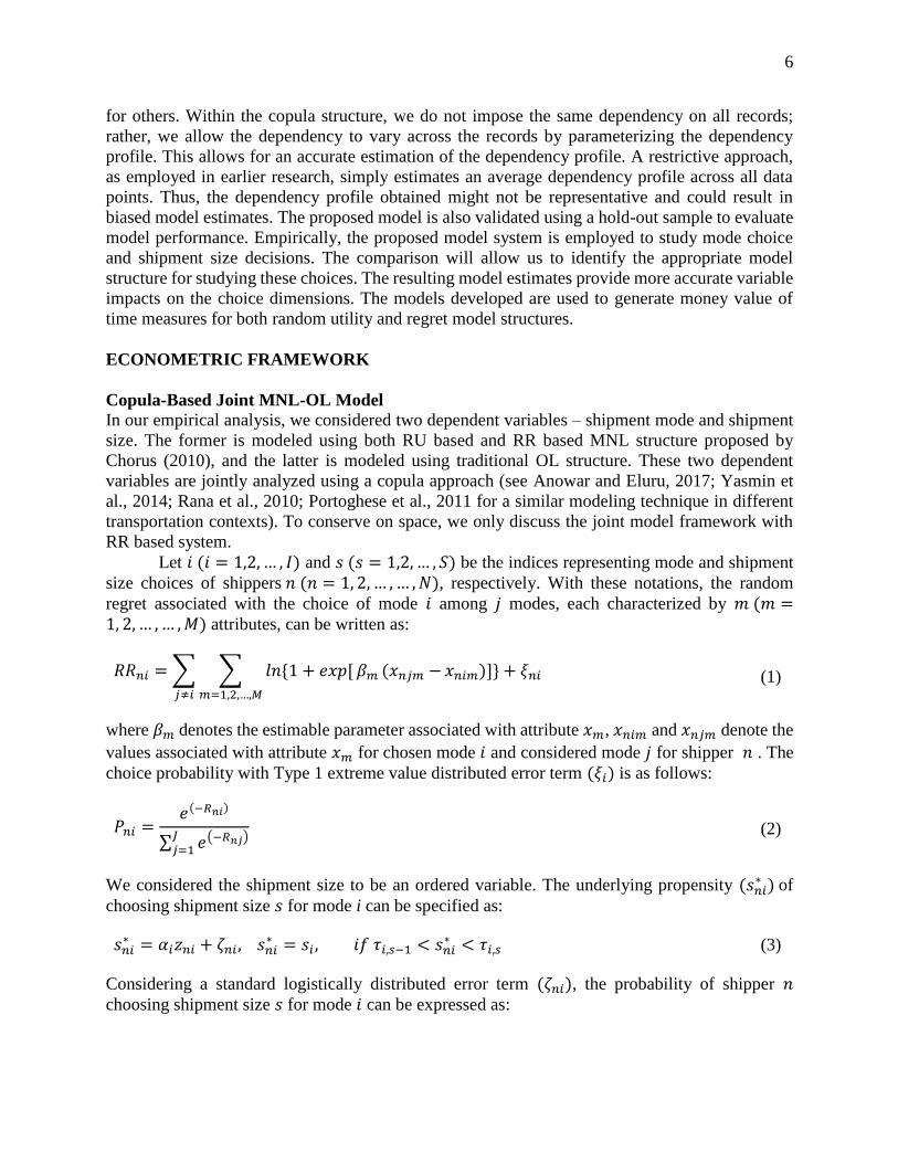
ECONOMETRIC FRAMEWORK
Copula-Based Joint MNL-OL Model
In our empirical analysis, we considered two dependent variables – shipment mode and shipment
size. The former is modeled using both RU based and RR based MNL structure proposed by
Chorus (2010), and the latter is modeled using traditional OL structure. These two dependent
variables are jointly analyzed using a copula approach (see Anowar and Eluru, 2017; Yasmin et
al., 2014; Rana et al., 2010; Portoghese et al., 2011 for a similar modeling technique in different
transportation contexts). To conserve on space, we only discuss the joint model framework with
RR based system.
Let 𝑖 (𝑖 = 1,2, … , 𝐼) and 𝑠 (𝑠 = 1,2, … , 𝑆) be the indices representing mode and shipment
size choices of shippers 𝑛 (𝑛 = 1, 2, … , … , 𝑁), respectively. With these notations, the random
regret associated with the choice of mode 𝑖 among 𝑗 modes, each characterized by 𝑚 (𝑚 =1, 2, … , … , 𝑀) attributes, can be written as:
𝑅𝑅𝑛𝑖 = ∑ ∑ 𝑙𝑛{1 + 𝑒𝑥𝑝 [ 𝛽𝑚
𝑚=1,2,…,𝑀
(𝑥𝑛𝑗𝑚 −
𝑗≠𝑖
𝑥𝑛𝑖𝑚)]} + 𝜉𝑛𝑖 (1)
where 𝛽𝑚 denotes the estimable parameter associated with attribute 𝑥𝑚, 𝑥𝑛𝑖𝑚 and 𝑥𝑛𝑗𝑚 denote the
values associated with attribute 𝑥𝑚 for chosen mode 𝑖 and considered mode 𝑗 for shipper 𝑛 . The
choice probability with Type 1 extreme value distributed error term (𝜉𝑖) is as follows:
𝑃𝑛𝑖 =𝑒(−𝑅𝑛𝑖)
∑ 𝑒(−𝑅𝑛𝑗)𝐽𝑗=1
(2)
We considered the shipment size to be an ordered variable. The underlying propensity (𝑠𝑛𝑖∗ ) of
choosing shipment size 𝑠 for mode i can be specified as:
𝑠𝑛𝑖∗ = 𝛼𝑖𝑧𝑛𝑖 + 𝜁𝑛𝑖 , 𝑠𝑛𝑖
∗ = 𝑠𝑖 , 𝑖𝑓 𝜏𝑖,𝑠−1 < 𝑠𝑛𝑖∗ < 𝜏𝑖,𝑠 (3)
Considering a standard logistically distributed error term (𝜁𝑛𝑖), the probability of shipper 𝑛
choosing shipment size 𝑠 for mode 𝑖 can be expressed as:

7
𝑃𝑛𝑖 = 𝛬𝑖(𝜏𝑖,𝑠 − 𝛼𝑖𝑧𝑛𝑖) − 𝛬𝑖(𝜏𝑖,𝑠−1 − 𝛼𝑖𝑧𝑛𝑖) (4)
where, 𝛬 represents the cumulative density function for standard logistic distribution,
𝜏𝑖,𝑠 (𝜏𝑖,0 = −∞, 𝜏𝑖,𝑆 = +∞) represents the thresholds associated with shipment size 𝑠 for mode 𝑖
with the following ordering condition (−∞ < 𝜏𝑖,1 < 𝜏𝑖,2 < ⋯ < 𝜏𝑖,𝑆−1 < +∞); 𝛼𝑖 are the
estimable parameters, 𝑧𝑛𝑖 are vector of attributes.
The shipment size and mode component may be coupled together through their stochastic
error terms using the copula approach. The joint distribution (of uniform marginal variables) can
be generated by a function 𝐶𝜃𝑛(. , . ) (Sklar, 1973), such that:
𝛬𝜉𝑛𝑖,𝜁𝑛𝑖(𝑈1, 𝑈2) = 𝐶𝜃𝑛
(𝑈1 = 𝛬𝜉𝑛𝑖(𝜉), 𝑈2 = 𝛬𝜁𝑛𝑖
(𝜁)) (5)
where 𝐶𝜃𝑛(. , . ) is a copula function and 𝜃𝑛 the dependence parameter defining the link between
𝜉𝑛𝑖 and 𝜁𝑛𝑖. Level of dependence between shipment mode and size might vary across shippers.
Recognizing that, we parameterize the dependence parameter 𝜃𝑛 as a function of freight
characteristics. The equation is:
𝜃𝑛 = 𝑓(𝛾𝑖𝜗𝑛𝑖) (6)
where 𝜗𝑛𝑖 is a column vector of exogenous variables, 𝛾𝑖 is a row vector of unknown parameters
(including a constant) specific to mode 𝑖 and 𝑓 represent the functional form of parameterization.
The parameterization was carefully done for each of the six copula types considering the
permissible limits of the dependency parameters. More specifically, for normal, FGM and Frank
copulas we use the following functional form:
𝜃𝑛 = 𝑓(𝛾𝑖𝜗𝑛𝑖) (7)
While for Clayton we use:
𝜃𝑛 = 𝑒𝑥𝑝(𝛾𝑖𝜗𝑛𝑖) (8)
and for Gumbel and Joe the function is:
𝜃𝑛 = 1 + 𝑒𝑥𝑝(𝛾𝑖𝜗𝑛𝑖) (9)
All the models are estimated by maximizing the log-likelihood function coded in GAUSS matrix
programming language. In our analysis, we employ six different copula structures – Gaussian
copula, Farlie-Gumbel-Morgenstern (FGM) copula, and a set of Archimedean copulas including
Frank, Clayton, Joe and Gumbel copulas (a detailed discussion of these copulas is available in
Bhat and Eluru, 2009). Please note that restricting the copula structure to have no correlation
between the error terms of shipping mode and shipment size choices would result in the
independent copula model.
EMPIRICAL DATA

8
Data Source and Data Preparation
The data for our analysis is drawn from the 2012 US CFS data available at
www.census.gov/econ/cfs/pums.html. This survey is the joint data collection effort of Bureau of
Transportation Statistics (BTS) and U.S. Census Bureau. The survey is conducted every 5 years
since 1993. Although several data sources are available for freight planning purposes, this is the
only freely available source that portray a detailed picture of freight movement at national level.
A total of 4,547,661 shipment records from approximately 60,000 responding businesses and
industries are recorded (including some important freight characteristics) in the Public Use
Microdata (PUM) file of the 2012 CFS. To reduce the data processing and model estimation
burden, a random sample of 15,000 records was carefully drawn from the PUM database ensuring
that the mode share of the extracted sample was the same as the weighted mode share of the
original database. From this sample, 10000 data records were randomly chosen for estimation and
5,000 records were set aside for validation exercise.
Dependent Variable Generation
The 2012 CFS PUM file reports twenty-one modes of transport. In this study, the reported modes
were categorized into five major groups: (1) for-hire truck, (2) private truck, (3) air, (4) parcel
service, and (5) "other mode". Here, for-hire truck mode represents the trucks operated by a non-
governmental business unit to provide transport services to customers under a negotiated rate. On
the other hand, private truck refers to trucks owned and used by an individual business entity for
its own freight movement. Parcel service mainly refers to a combination of modes (on
ground/air/express carrier). Air mode consists of both air and truck, as truck is needed to pick up
and/or deliver the commodity from and/or to a particular place which cannot be accessed by air
mode. The other mode consists of rail, water, pipeline or combination of non-parcel multiple
modes. The weighted mode share by number of shipments in the estimation sample is as follows:
for-hire truck (16.47%), private truck (26.23%), parcel (55.64%), air (1.36%), and other (0.29%).
The reader would note that certain types of shipments can be transported by only a subset of the
modes. For instance, it is very unlikely that a large load of 50 tons is shipped by air or parcel mode
as these modes have capacity restrictions. Therefore, allowing air or parcel mode as an available
option for such shipments affects the accuracy of the model estimates. To account for this issue, a
heuristic approach was adopted to define the mode availability option based on shipment weight
and routed distance (see Keya et al., 2017 for details). After carefully examining the freight
characteristics of the chosen mode, following guidelines have been developed for alternative
availability: for-hire truck and other mode have been considered always available; private truck is
set available when routed distance is less than 413 miles (99 percentile of private truck observed
in the data); air and parcel mode are considered available when shipment weight is less than 914
lb and less than 131 lb respectively (99 percentile observed in the data).
Shipment size is reported as a continuous variable in the CFS data. In our study, we
categorized it into seven groups from very small to very large shipment size based on the observed
frequency distribution of shipment size from the CFS data. We have categorized the shipment size
in such a way that there exists a reasonable share of shipment size in each category for each
shipping mode. These are: (1) category 1 (<=30 lb), (2) category 2 (30-200 lb), (3) category 3
(200-1,000 lb), (4) category 4 (1,000-5,000 lb), (5) category 5 (5,000-30,000 lb), (6) category 6
(30,000-45,000 lb), and (7) category 7 (> 45,000 lb). Table 2 presents the weighted distribution of
shipment sizes across five modes considered by number of shipments. We can see from the table
that across for-hire truck and private truck modes; the shipment sizes are quite evenly distributed

9
with the highest percentage share for 5,001-30,000 lb category for for-hire truck (18.59%) and for
201-1,000 lb category for private truck (19.46%). Therefore, for for-hire and private truck, we
considered all seven of the shipment size categories. It is also evident from the table that air and
parcel modes primarily carry smaller shipments weighing less than 30 lb (59.6% and 78.81%,
respectively). Hence, only two categories of shipment size were assigned to air and parcel mode –
less than or equal to 30 lb and greater than 30 lb. We can also see that the other mode mainly
contains large shipment sizes in categories 6 and 7. Since other mode consists primarily of rail,
this is expected. Based on weight distributions, for other mode, we considered three shipment size
categories (less than or equal to 30 lb (3.06%), 31-5,000 lb (9.17%), and greater than 5,000 lb
(87.78%). Table 3 presents the weighted mode share across the seven shipment size groups. It can
be observed from the table that in general truck modes have the largest share across all shipment
sizes (except when shipment size is less than 200 lb). On the other hand, air and parcel mode
mainly carry smaller shipment size (less than 200 lb). It is also clear from the table that other mode,
which is dominated by rail, transports larger shipment size. The distribution clearly shows how by
mode, shipment size varies substantially highlighting the potential interconnectedness.
Independent Variable Generation
While the CFS data contains important freight attributes, level of service (LOS) variables, such as
shipment time and shipment cost, are not available in the data. Therefore, we augmented the data
with a host of secondary data sources. First, LOS variables were generated for each mode based
on the origin and destination locations, routed distance and the shipment weight reported in the
data. We generated shipping time for for-hire and private truck considering three different travel
speed bands based on trip distance. In this procedure, we also considered the required break times
for the truck drivers according to the service regulations, suggested by Federal Motor Carrier
Safety Administration (FMCSA). Based on the share of shipping speed from FedEx 2015 annual
report, we generated the shipping time by parcel mode- express overnight (1day), express deferred
(3 days) and ground service (5days). Shipping time of air and “other mode” (considering rail, as
rail contains major share within other mode) was calculated based on the average speed obtained
from different sources. For shipping cost by parcel mode we developed pricing functions
considering shipping distance and shipment weight and using shipping cost information available
from FedEx. We also considered the shipping speed in calculation of shipping cost by parcel mode
based on the share of shipping speed from FedEx 2015 annual report. Shipping cost for for-hire
truck, private truck and “other mode” (mainly rail) was calculated based on the 2007 average
freight revenue information obtained from the National Transportation Statistics (NTS) website
with appropriate regional and temporal correction factors. The shipping cost per pound for air was
estimated based on cost documentation obtained from a U.S. based cargo company- Southwest
Cargo Company. For more details on level of service generations see Keya et al, 2017. Second, a
number of O-D attributes were compiled utilizing different sources which include National
Transportation Atlas Database (NTAD) 2012, National Bridge Inventory (NBI) data, National
Highway Freight Network (NHFN) data, Highway Performance Monitoring System (HPMS) data,
and Freight Analysis Framework – version 4 (FAF4) network data. The transportation network
attributes generated are: roadway length per functional classification (interstate highway, freeway
and expressway, principal arterial, minor arterial, major and minor collector), railway length,
number of airports, number of seaports, number of intermodal facilities, number of bridges, truck
annual average daily traffic (AADT), length of tolled road, length of truck route, and length of
intermodal connectors. Several CFS zonal level variables (both at origin and destination) have also

10
been generated including population density, number of employees and number of establishments
by North American Industry Classification System (NAICS) (manufacturing, mining, retail trade,
warehouse and storage, company and enterprise, wholesale, information), income categories based
on mean income of an area (low (< $50,000), medium ($50,000-$80,000) and high (>$80,000)),
number of warehouses and super centers, major industry type in an area (based on the majority of
existing industries in an area), percentage of population below poverty level, and annual average
temperature (www.currentresults.com/Weather/US/average-annual-state-temperatures.php) (cold
if the average annual temperature is less than or equal to 60oF; warm if the temperature is greater
than 60oF). To generate the zonal level variables, at first we collected the county level data. Then,
we aggregated these information from the counties within each CFS area to obtain the CFS area
level data.
Descriptive Statistics
Table 4 of descriptive analysis of the estimation sample reveals that the majority of the shipments
are domestic – transported within the US (95.8%). Moreover, the shipment shares of both
temperature controlled products and hazardous materials are very low (4.7% each) compared to
other commodity types. We also found that most of the shipments are originating and terminating
in non-mega regions1 (36.1% and 33.9%, respectively). The most commonly shipped commodity
types by frequency of shipment in 2012 were electronics (20.2%), metals and machinery (18.8%),
and wood, paper and textiles (17.9%). The least transported commodity type was stone and non-
metallic minerals (2.1%) and raw food (2.6%). The percentage share of shipment by value is the
highest for shipment value less than $300 (44.5%). The mean shipping cost is the highest ($276.53)
for air mode, with the lowest mean shipping time (1.30 hours). On the other hand, shipping cost is
the lowest for other modes ($13.71) and mean shipping time is the highest for parcel mode (98.84
hours).
EMPIRICAL ANALYSIS
Model Fit A series of models were estimated in the current study. First, we developed independent discrete
choice models of mode and shipment size choice. For mode choice analysis, both RU based as
well as RR based MNL models were estimated while for shipment size we estimated traditional
OL models for each mode. The log-likelihood values of the independent models can be
appropriately summed up to obtain the independent copula model log-likelihood. These models
were estimated to establish a benchmark for model performance evaluation. Second, we estimated
a copula-based joint mode and shipment size choice model considering both decision rules for the
mode choice decision. In our study, we considered six different copula structures: (1) Gaussian,
(2) FGM, (3) Clayton, (4) Gumbel, (5) Frank, and (6) Joe. We also estimated models allowing
different dependency structures (for example Frank copula for the first three mode types, and Joe
copula for parcel mode). Third, rather than imposing a single dependency parameter across the
dataset, we allow for the copula dependency to vary as a function of exogenous variables. Please
1 The entire USA is divided into eleven megaregions which are expected to share common economic growth, natural
resources and environmental system, topography, and transportation system. These eleven megaregions are: Arizona
Sun Corridor, Cascadia, Florida, Front Range, Great Lakes, Gulf Coast, Northeast, Northern California, Piedmont
Atlantic, Southern California, and Texas Triangle. The remainder of the USA has been considered as non-mega region
(http://www.america2050.org/content/megaregions.html).

11
note that we did not estimate any dependency parameter for “other” mode since it had too few
observations for model estimation. Finally, to determine the most suitable copula model (including
the independent copula model), a comparison exercise was undertaken.
Since the alternative copula models are non-nested, we compared their performance using
Bayesian Information Criterion (BIC) and Akaike Information Criterion (AIC). The BIC value for
a given empirical model can be calculated as: [– 2 (𝐿𝐿) + 𝐾 𝑙𝑛 (𝑄)], where 𝐿𝐿 is the log-
likelihood value at convergence, 𝐾 is the number of parameters and 𝑄 is the number of
observations. While, AIC value is calculated using the following equation for a given empirical
model: [2 𝐾 − 2 𝑙𝑛 (𝐿𝐿)], where K is the number of parameters and LL is the log likelihood at
convergence. The model with the lowest BIC and AIC value is the preferred model. The BIC and
AIC values obtained are presented in Table 5. We can see from the table that the combination of
Frank-Frank-Frank-Joe-Independent for RRM based MNL-OL copula provided the best data fit.
The BIC (number of parameters) values for the RRM based MNL-OL Frank-Frank-Frank-Joe-
Independent copula model and independent model are 25762.57 (94) and 26473.42 (99),
respectively. From the RU regime as well, a similar combination of copulas (Frank-Frank-Frank-
Joe-Independent) provided the best data fit (25765.36 (93)). Also, the AIC (no. of parameters)
values for the RRM based and RU based MNL-OL Frank–Frank-Frank-Joe-Independent copula
model are 25084.80(94) and 25094.80(93) respectively. The BIC and AIC values indicate that the
random regret based copula model outperformed its random utility counterpart. The copula model
BIC and AIC comparisons confirms the importance of accommodating dependence between mode
type and shipment size choice dimensions in the analysis of freight mode choice. In addition, we
found that the RRM based copula model (Frank-Frank-Frank-Joe-Independent) with
parameterization provided the best data fit amongst all the copulas (BIC value: 25713.41 (98) and
AIC value: 25006.80(98)). Therefore, in the subsequent sections, we will only discuss about the
results for this model. In our analysis, variable selection was guided by a 90 percent significance
level and variable impact expectations from past research.
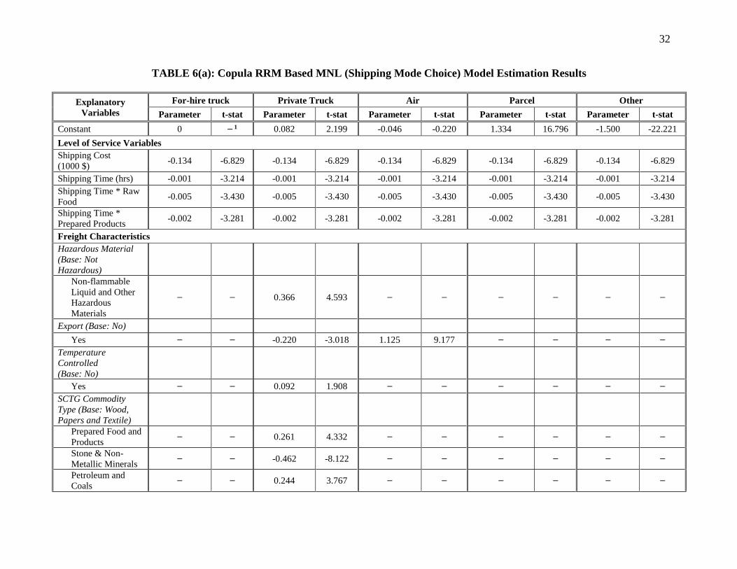
Mode Choice Component Table 6(a) represents the results of the RR based mode choice component. A positive (negative)
sign for the coefficients indicates that an increase (decrease) in the corresponding attribute
increases (decreases) the regret associated with not participating in the alternative and contributes
to an increase (decrease) in the probability for participating in the alternative. In the following
section, the estimation results are discussed by variable groups.
Level of Service Variables
In our empirical analysis, shipment time and cost variables have negative coefficients (-001 per
hour and -0.134 per $1000 respectively) indicating that regret is higher if the competitor mode has
lower travel time or lower shipment cost (see Boeri and Masiero, 2014 for similar results). In our
model, we also tested for several first order interactions of travel time with commodity types; only
two interactions were significant. The signs of the coefficients of the interaction terms of shipping
time with raw food and prepared products are found to be intuitive. Relative to other commodities,
shipping of these two commodities are more time sensitive as indicated by worsening regret with
increase in travel time. The magnitude of sensitivity is larger for raw food commodity. This result
is reasonable because raw food products are perishable and require timely delivery.
Freight Characteristics

12
The effects of the freight attributes provide interesting results. Both non-flammable liquid and
other hazardous materials, and temperature controlled products are more likely to be shipped by
private truck. These type of shipments require special handling and safety precautions which can
be accommodated by private truck operators. In addition, temperature controlled products can be
delivered to its destination without any transfer time (as required for other modes). The value of
the coefficient for export trade by air mode is 1.125, which implies that air is the preferred mode
for transporting export shipments. It is expected, as shipping overseas is more convenient by air
mode (see Wang et al., 2013 for similar result). However, the coefficient for export trade by private
truck (-0.220) indicates that, it is less likely that private truck would be chosen for export purposes
as private trucks are more likely to be used for shorter shipping distances. Private truck is preferred
for commodities such as prepared food and products, petroleum and coal, and furniture and other
miscellaneous commodities. Private trucks are more likely to be used to carry small quantities of
refined petroleum to the gasoline distribution locations, such as gas stations within shorter
distances. On the other hand, private truck is less preferred for transporting stone and non-metallic
minerals and electronic products. Air mode is preferred for transporting electronic products which
are lightweight, costly and require special care to prevent any damage due to shock while
transporting. Similar finding is reported by Pouraabdollahi et al. (2013a). In terms of shipment
value, for shipments valued under $5000, private truck is more likely to be chosen. Regret
gradually decreases for higher value merchandise (see Sayed and Razavi, 2000; Norojono and
Young, 2003; Arunotayanun and Polak, 2011; Moschovou and Giannopoulos, 2012 for similar
findings).
Transportation Network and O-D Attributes
Private truck is less preferred when the density of railways or number of intermodal facilities at
destination zone increases. The possibility of choosing air mode decreases when density of railway
at origin increases (coefficient value: -0.88) or when the percentage of population living below
poverty level is high at origin (coefficient value: -4.006). Air mode is typically expensive and
hence, shippers in the impoverished regions are less likely to ship/receive products by this mode.
Higher population density is a proxy for higher demand for service. Hence, with increasing
population density at destination CFS zone, the probability of choosing air and parcel mode
increases. If shipment’s originating zone has higher highway density or increased number of
warehouse and supercenters parcel mode is also more likely to be chosen. The result is expected
because parcel mode requires greater accessibility through roadway network. Moreover,
warehouses are generally situated in locations with better highway accessibility, allowing for faster
access by parcel mode. However, parcel mode is less preferred when the density of wholesale
industry at origin increases (coefficient value: -0.091); possibly because wholesale industries
generally ship bulk loads and for bulk loads, parcel is not a convenient mode option.
Shipment Size Component The results of ordered logit models for each mode type are presented in Table 6(b). A positive
(negative) coefficient increases (decreases) the shipper’s propensity for choosing a larger (smaller)
shipment size category. The results are discussed by variable groups in the following section.
Please note that the threshold variables do not have any substantive interpretation.
Freight Characteristics

13
The coefficient (0.946) of non-flammable liquid and other hazardous materials indicates that, these
products are more likely to be shipped in larger volume using for-hire trucks. Trucks can be
specially equipped and operated to carry hazardous materials to ensure safe transportation of such
commodities. As expected, shipment size of commodities requiring temperature control
(coefficient value: -0.853) is likely to be smaller for parcels as it may not be able to offer the special
handling care required for these commodities. Commodities, such as raw food, prepared products,
stone and non-metallic minerals, and petroleum and coals, are likely to be shipped in large amounts
by for-hire and private trucks. Both for-hire and private trucks offer unhindered movement of these
commodities without needing any transfers. On the other hand, chemicals, furniture and other
products might be shipped in smaller quantities when using private truck as a mode of
transportation. Also, electronics tend to be shipped in smaller amounts by for-hire truck, private
truck, air and parcel modes. Parcel mode may have weight restrictions for shipping; hence,
shipment size for furniture, and metals and machinery are likely to be on the smaller side.
However, for prepared products, the shipment sizes are likely to be on larger side. Shipment value
and its size are negatively correlated for all modes.
Transportation Network and O-D Attributes
Several transportation networks and O-D attributes were considered in the shipment size models.
For for-hire truck, density of employees in mining industry at origin increased the propensity for
larger shipments. This possibly reflects the nature of industry in the region. In addition, density of
bridges at destination, cold climate at origin (average annual temperature ≤600F), and increased
routed distance reduces the propensity for large shipments using for-hire trucks. For private truck,
density of highways in the destination zone (coefficient value: 0.617) increases the propensity for
larger shipments since increased roadway coverage facilitates movement of goods in large
quantity. On the other hand, density of management companies and enterprises at destination
decreases the propensity for large shipments, as this type of establishments normally attracts
commodities with smaller weight including office supplies and electronics. For parcel mode, the
propensity of large shipment increases when mean zonal income at origin is less than $50,000.
However, increased density of wholesale industries at destination (coefficient value: -0.094) or
increased number of seaports at origin (coefficients value: -0.001) reduces the propensity for large
shipments by parcel mode. Wholesale industries potentially generate bulk weight that is less
convenient to be transported by parcel mode. Shipping large amount of freight through seaports is
cost effective.
Copula Parameters
The last panel of Table 6(b) presents the copula parameters estimated. The statistically significant
dependency parameters imply the existence of unobserved factors strongly influencing the mode
and shipment size choice decision simultaneously. Further, the results clearly highlight how the
dependence varies across the dataset. The Frank copula is associated with for-hire truck, private
truck, and air modes while Joe copula is associated with parcel mode. For the “other” mode
alternative, dependency could not be captured due to the small sample size. The Frank copula
provides symmetric dependency; i.e. the positive copula parameter specifies that the dependency
caused by the common unobserved factors for the specific mode is positive, and a negative copula
specifies that the dependency is negative. In our case, the constant parameter in Frank is negative
indicating that the common unobserved factors that increase the probability of choosing the mode
are likely to reduce the probability that larger shipment size is chosen. The Joe copula is only

14
associated with positive dependency and proposes a stronger right tail dependency. The positive
sign of Joe copula associated with parcel mode implies that the common unobserved factors that
increase the propensity of choosing parcel mode also increase the propensity of choosing a larger
shipment size. Several freight characteristics influence the dependency across the mode and
shipment size categories. The variables include raw food, stone and non-metallic minerals,
shipment value less than $300 and shipment value from $300 to $1000 (for-hire truck); metals and
machinery (private truck); and export trade type (parcel). The parameter values provide
customized dependency values across the dataset. The reader would note that accounting for the
flexible specification for common unobserved factors enhances model fit. At the same time, it is
important to recognize that ignoring for the presence of these common unobserved factors is likely
to result in biased and/or inconsistent estimates for all other parameters. Hence, the copula model
offers a twofold benefit: (1) improve model fit and (2) allows for enhanced parameter estimation
of the data under consideration.
Model Validation
To evaluate the performance of the estimated models, we also performed a validation exercise.
Specifically, we employed the final parameters obtained from the models to compute the predictive
log-likelihood (LL) and BIC values for four models: (1) RRM based MNL-OL Copula (Frank-
Frank-Frank-Joe-Independent) with parameterization, (2) RUM based MNL-OL Copula (Frank-
Frank-Frank-Joe-Independent) with parameterization, (3) RRM based MNL-OL Independent
Copula, and (4) RUM based MNL-OL Independent Copula. The results are reported in Table 7.
The overall predictive log-likelihood and BIC values clearly indicate that RR based MNL-OL
copula (Frank-Frank-Frank-Joe) with parameterization performs better than other models. Further,
to illustrate the performance, we generate predicted LL values for several sub-samples including
freight characteristics such as flammable liquid, commodity type (such as raw food, prepared
products, chemicals). Except for a few instances, the RRM based MNL-OL copula model offers
improved fit in the majority of the cases. Overall, the validation results also confirm the value of
considering dependency across mode choice and shipment size. A prediction exercise has been
conducted to compare actual and predicted mode and shipment size share. From Figure 2, we can
clearly observe that the actual and predicted mode share are almost similar indicating a satisfactory
predictive ability of our model. The predicted shipment size share has been provided in Table 8
and the results are quite reasonable highlighting the appropriateness of the joint model.
Value of Time (VOT)
We also have estimated the value of time (VOT). In the random regret minimization approach,
the value of time (VOT) is calculated using the following equation (Chorus, 2012):
VOT = ∑ −βt/(1+1/exp [βt(TTj−TTi)]))j≠i
∑ −βc/(1+1/exp [βc(TCj−TCi)]))j≠i (10)
Where, βt and βc are the estimated coefficients of shipping time and shipping cost respectively. In
the RRM based approach, the shipping time and shipping cost of both the chosen alternative and
the competitor alternatives enter into the VOT equation. Figure 3 represents the value of time
analysis across different modes, where the blue plane with a single value represents VOT obtained
from RUM model and the colored plane with varying values represents VOT values obtained from
RRM model. From the figure, we can observe that the VOT obtained from random utility model
in not sensitive to any change in the attributes. However, random regret formulation based VOT

15
changes across the mode and is affected by the change in attribute levels. The results from VOT
analysis highlight that while RUM and RRM based analysis provide similar ranges of VOT, the
inherent variation allowed in RRM models enhances data fit.
In our analysis, we also calculated the VOT per ton using the weighted average shipment
weight across all modes (4.93 ton). Based on the data used to generate Figure 3, the VOT per ton
for RRM based model results in different range of values. For for-hire truck and private truck the
VOT per ton value ranges between 1.50 to 1.52; for air this value ranges between 1.48 to 1.49; for
parcel VOT per ton ranges between 1.56 and 1.65; and for other mode this value ranges between
1.50 to 1.57. The value of VOT per ton for the RUM based analysis is obtained as 1.50 (same for
all modes). The range of VOT per ton values are reasonable and are similar to values reported in
earlier literature. For example, Fowkes et al. (1991) and Kurri et al. (2000) found the values as
€1.18 ($1.33) per ton and €1.53 ($1.73) per ton respectively, whereas de Jong et al. (2004) found
a comparatively higher value of €4.7 ($5.36) per ton.
CONCLUSION
In our study, a joint model system is developed in the form of an unordered choice model for mode
and an ordered choice model for shipment size. We adopt a closed form copula-based model
structure for capturing the impact of common unobserved factors affecting these two choices. We
explore both the random utility (RU) based multinomial logit and the random regret (RR)
minimization based multinomial logit (MNL) within a copula-based model. The RU and RR MNL
structure are explored for several copula-based structures including Gaussian, Farlie-Gumbel-
Morgenstern (FGM), Clayton, Gumbel, Frank and Joe. Finally, we consider six different copula
structures while allowing for different copula structures within the same model (as opposed to a
single copula form for all dimensions). For all the copula models, a more flexible approach that
allows for exogenous variables to influence dependency structure is also estimated. The models
are estimated based on the data from 2012 Commodity Flow Survey data. The estimated results
obtained from this study clearly indicates the importance of accommodating dependencies between
shipment mode and shipment size choice decisions. Of the copula models, RR based MNL-OL
Frank-Frank-Frank-Joe copula model with parameterization offered the best fit. The estimated
coefficients exhibited plausible interpretations too. The validation exercise performed to evaluate
the model fit for overall sample and sub-samples based on freight characteristics suggests that RR
based MNL-OL copula (Frank-Frank-Frank-Joe-Independent) model with parameterization
significantly outperforms other models.
Certain drawbacks of this study need to be acknowledged. PUM CFS data does not contain
exact geo-coded locations of origin and destination of freight movement. Advanced approaches to
augment the data set with this information will improve the calculation of LOS variables and
alternative availability matrices. Any information of trip chaining or intermediate modes used
sequentially in a particular shipping trip from one origin to destination is also not available in the
dataset. Availability of such information in future, will enhance the model estimation results.
Additionally, evidence of shipper level reliability, shipment frequency, shipping time delay,
ownership of the vehicle fleet by the shipping firms will enhance the model results. In the future,
accommodating more detailed land use attributes will provide the policy makers more interesting
insights.
In terms of econometric methodology, two possible challenges can be fruitful avenues for
future research. First, to accommodate the inherent discretization of the shipment size variable we
developed the ordered logit model that provides additional flexibility by allowing for a non-linear

16
specification (as opposed to linear model). However, the approach can result in loss of information
as we convert the continuous value to a discrete variable. In scenarios where the loss of information
is likely to be a challenge, it might be useful to consider increasing the number of alternatives in
modeling shipment size and estimating an advanced version of the ordered logit (see Rahman et
al., 2019 for an example). Second, the dependency of copula model does not accommodate for
random taste variations attribute impacts. Therefore, accommodating random taste variations
within a copula based structure may be an avenue for future research.

17
REFERENCES
Abdelwahab, W.M. and Sargious, M. (1990). Freight rate structure and optimal shipment size in
freight. Logistics and Transportation Review, 26(3), p.271.
Abdelwahab, W., & Sargious, M. (1992). Modelling the demand for freight transport: A new
approach. Journal of Transport Economics and Policy, 49-70.
Abdelwahab, W. M. (1998). Elasticities of mode choice probabilities and market elasticities of
demand: Evidence from a simultaneous mode choice/shipment-size freight transport model.
Transportation Research Part E: Logistics and Transportation Review, 34(4), 257-266.
Abdelwahab, W., & Sayed, T. (1999). Freight mode choice models using artificial neural
networks. Civil Engineering Systems, 16(4), 267-286.
Abate, M., & de Jong, G. (2014). The optimal shipment size and truck size choice–The allocation
of trucks across hauls. Transportation Research Part A: Policy and Practice, 59, 262-277.
Anderson, W. P., Chatterjee, L., & Lakshmanan, T. (2003). E‐commerce, transportation, and
economic geography. Growth and Change, 34(4), 415-432.
Anowar, S., & Eluru, N. (2017). Univariate or Multivariate Analysis for Better Prediction
Accuracy? A Case Study of Heterogeneity in Vehicle Ownership. Forthcoming
Transportmetrica A: Transport Science.
Arunotayanun, K., & Polak, J. W. (2011). Taste heterogeneity and market segmentation in freight
shippers’ mode choice behaviour. Transportation Research Part E: Logistics and
Transportation Review, 47(2), 138-148.
Arentze, T., & Timmermans, H. (2007). Parametric action decision trees: Incorporating continuous
attribute variables into rule-based models of discrete choice. Transportation Research Part
B: Methodological, 41(7), 772-83.
Ben-Akiva, M. E., & Lerman, S. R. (1985). Discrete choice analysis: Theory and application to
travel demand. MIT press.
Bhat, C. R., & Eluru, N. (2009). A copula-based approach to accommodate residential self-
selection effects in travel behavior modeling. Transportation Research Part B:
Methodological, 43(7), 749-765.
Boeri, M., & Masiero, L. (2014). Regret minimisation and utility maximisation in a freight
transport context. Transportmetrica A: Transport Science, 10(6), 548-560.
Cavalcante, R., & Roorda, M. J. (2010). A disaggregate urban shipment size/vehicle-type choice
model. In Transportation Research Board 89th Annual Meeting, Washington, D. C., 2010.
Chakour, V., & Eluru, N. (2016). Examining the influence of stop level infrastructure and built
environment on bus ridership in Montreal. Journal of Transport Geography, 51, 205-217.
Chorus, C. G., Arentze, T. A., & Timmermans, H. J. P. (2008). A random regret-minimization
model of travel choice. Transportation Research Part B: Methodological, 42(1),1-18.
Chorus, C. G. (2010). A new model of random regret minimization. EJTIR, 10 (2), 2010.
Combes, F. (2012). Empirical evaluation of economic order quantity model for choice of shipment
size in freight transport. Transportation Research Record: Journal of the Transportation
Research Board (2269), 92-98.
Current Results. Weather and science facts. The average annual temperature for each US state.
https://www.currentresults.com/Weather/US/average-annual-state-temperatures.php.
Accessed March 8, 2018.
De Jong, G., Kroes, E., Plasmeijer, R., Sanders, P., & Warffemius, P. (2004). New values of time
and reliability in freight transport in The Netherlands. Paper presented at the European
Transport Conference, Strasbourg.
18
De Jong, G., & Ben-Akiva, M. (2007). A micro-simulation model of shipment size and transport
chain choice. Transportation Research Part B: Methodological, 41(9), 950-965.
De Jong, G., & Johnson, D. (2009). Discrete mode and discrete or continuous shipment size choice
in freight transport in Sweden. Paper presented at the European transport conference,
Noordwijkerhout, The Netherlands.
Freight Shipments in America. U.S. Department of Transportation. Bureau of Transportation
Statistics, 2004.
https://www.rita.dot.gov/bts/sites/rita.dot.gov.bts/files/publications/freight_shipments_in_a
merica/index.html. Accessed online on March 8, 2018.
Fowkes, A., Nash, C., & Tweddle, G. (1991). Investigating the market for inter-modal freight
technologies. Transportation Research Part A: General, 25(4), 161-172.
Habibi, S. (2010). A discrete choice model of transport chain and shipment size on Swedish
commodity flow survey 2004/2005.
Hall, R. W. (1985). Dependence between shipment size and mode in freight transportation.
Transportation Science, 19(4), 436-444.
Holguín-Veras, J. (2002). Revealed preference analysis of commercial vehicle choice process.
Journal of Transportation Engineering, 128(4), 336-346.
Holguín-Veras, J., Xu, N., De Jong, G., & Maurer, H. (2011). An experimental economics
investigation of shipper-carrier interactions in the choice of mode and shipment size in freight
transport. Networks and Spatial Economics, 11(3), 509-532.
Irannezhad, E., Prato, C. G., Hickman, M., & Mohaymany, A. S. (2017). Copula-based joint
discrete-continuous model of road vehicle type and shipment size. Transportation Research
Record: Journal of the Transportation Research Board (2610), 87-96.
Jiang, F., Johnson, P., & Calzada, C. (1999). Freight demand characteristics and mode choice: An
analysis of the results of modeling with disaggregate revealed preference data. Journal of
Transportation and Statistics, 2(2), 149-158.
Kahneman, D., & Tversky, A. (1979). Prospect theory: An analysis of decision under risk.
Econometrica. Journal of the Econometric Society, 263-91.
Keya, N., Anowar, S., & Eluru, N. (2017). Estimating a freight mode choice model: A case study
of commodity flow survey 2012. Presented at Transportation Research Board 96th Annual
Meeting, Washington, D.C., 2017.
Keya, N., Anowar, S., & Eluru, N. Freight Mode Choice: A Regret Minimization and Utility
Maximization Based Hybrid Model. Presented at the Transportation Research Board 97th
Annual Meeting, Washington, D.C (No. 18-06118).
Kivetz, R., Netzer, O., & Srinivasan, V. (2004). Alternative models for capturing the compromise
effect. Journal of Marketing Research, 41(3), 237-57.
Kurri, J., Sirkiä, A., & Mikola, J. (2000). Value of time in freight transport in Finland.
Transportation Research Record: Journal of the Transportation Research Board (1725), 26-
30.
Leong, W., & Hensher, D. A. (2015). Contrasts of relative advantage maximisation with random
utility maximisation and regret minimisation. Journal of Transport Economics and Policy
(JTEP), 49 (1), 167-86.
McFadden, D. (1974). The measurement of urban travel demand. Journal of Public Economics,
3(4), 303-28.
McFadden, D., and K. Train (2000). Mixed MNL models for discrete response. Journal of applied
Econometrics, 15 (5), 447-470.

19
Megaregions. America 2050. http://www.america2050.org/content/megaregions.html. Accessed
online May 19, 2018.
Mokhtarian, P. L. (2004). A conceptual analysis of the transportation impacts of B2C e-commerce.
Transportation, 31(3), 257-284.
Moschovou, T., & Giannopoulos, G. (2012). Modeling freight mode choice in Greece. Procedia-
Social and Behavioral Sciences, 48, 597-611.
Norojono, O., & Young, W. (2003). A stated preference freight mode choice model.
Transportation Planning and Technology, 26(2), 1-1.
Pourabdollahi, Z., Karimi, B., & Mohammadian, A. (2013a). Joint model of freight mode and
shipment size choice. Transportation Research Record: Journal of the Transportation
Research Board 2378), 84-91.
Pourabdollahi, Z., Javanmardi, M., Karimi, B., Mohammadian, A., & Kawamura, K. (2013b).
Mode and Shipment Size Choice Models in the FAME Simulation Framework. In
Transportation Research Board 92nd Annual Meeting, Washington, D.C., 2013.
Portoghese, A., Spissu, E., Bhat, C. R., Eluru, N., & Meloni, I. (2011). A copula-based joint model
of commute mode choice and number of non-work stops during the commute. International
Journal of Transport Economics/Rivista internazionale di economia dei trasporti, 337-362.
Rahman, M., Yasmin, S., & Eluru, N. (2019). Evaluating the Impact of a Newly Added Commuter
Rail System on Bus Ridership: A Grouped Ordered Logit Model Approach forthcoming
Transportmetrica A: Transport Science , 1-24.
Rana, T., Sikder, S., & Pinjari, A. (2010). Copula-based method for addressing endogeneity in
models of severity of traffic crash injuries: application to two-vehicle crashes. Transportation
Research Record: Journal of the Transportation Research Board (2147), 75-87.
Sklar, A. (1973). Random variables, joint distribution functions, and copulas. Kybernetika, 9(6),
449-460.
Sayed, T., & Razavi, A. (2000). Comparison of neural and conventional approaches to mode
choice analysis. Journal of Computing in Civil Engineering, 14(1), 23-30.
Stinson, M., Pourabdollahi, Z., Livshits, V., Jeon, K., Nippani, S., & Zhu, H. (2017). A joint model
of mode and shipment size choice using the first generation of Commodity Flow Survey
Public Use Microdata. International Journal of Transportation Science and Technology, 6(4),
330-343.
Swait, J. (2001). A non-compensatory choice model incorporating attribute cutoffs.
Transportation Research Part B: Methodological, 35(10), 903-928.
Train, K. E. (2009). Discrete choice methods with simulation. Cambridge University Press.
Tversky, A., & Kahneman, D. (1992). Advances in prospect theory: Cumulative representation of
uncertainty. Journal of Risk and Uncertainty, 5(4), 297-323.
Wang, Y., Ding, C., Liu, C., & Xie, B. (2013). An analysis of Interstate freight mode choice
between truck and rail: A case study of Maryland, United States. Procedia-Social and
Behavioral Sciences, 96, 1239-1249.
Windisch, E., De Jong, G., Van Nes, R., & Hoogendoorn, S. (2010). A disaggregate freight
transport model of transport chain and shipment size choice. In ETC 2010: European
Transport Conference, Glasgow, UK, 11-13 October 2010, Association for European
Transport (AET).
Yasmin, S., Eluru, N., Pinjari, A. R., & Tay, R. (2014). Examining driver injury severity in two
vehicle crashes–A copula based approach. Accident Analysis & Prevention, 66, 120-
135.Zhang, R. and Zhu, L. (2018). Threshold incorporating freight choice modeling for

20
hinterland leg transportation chain of export containers. Transportation Research Part A:
Policy and Practice.

21
FIGURE 1: Frequency Distribution of Shipment Size (lbs)
0
200
400
600
800
1000
1200
0
20
40
60
80
250
125
0
700
0
185
00
285
00
385
00
Fre
quen
cy
Shipment Size (lbs)

22
FIGURE 2: Actual vs. Predicted Mode Share
0.00
10.00
20.00
30.00
40.00
50.00
60.00
For-hire
Truck
Private
Truck
Air Parcel Other
Per
centa
ge
Shar
e
Shipping Mode
Actual
Predicted

23
(a) For-Hire Truck (b) Private Truck (c) Air
(d) Parcel (e) Other Mode
FIGURE 3: VOT for Different Shipping Modes

24
TABLE 1: Previous Literature on Joint Modeling of Freight Mode Choice and Shipment Size
Study Study
Area
Data
Type1 Methodology2 Decision
Variable
Modes
Considered3
Independent Variables Considered
Level of
Service
Measures
Freight
Characteristics
Network
and O-D
Attributes
Other
Characteristics
Hall (1985) USA − 4
Cost equations
for alternative
modes
Mode,
shipment
size
Truck, parcel Cost, time − Distance −
Abdelwahab
and Sargious
(1992)
USA RP
Switching
simultaneous
equations
(binary probit
for mode choice
and linear
regression for
shipment size)
Mode,
shipment
size
Truck, rail Cost, time
Shipment size,
commodity
density, value,
commodity type,
hazardous,
temperature
controlled
Destination
territory
Loss and
damage
percentage,
reliability
Abdelwahab
(1998) USA RP
Switching
simultaneous
equations
(binary probit
for mode and
linear
regression for
shipment size)
Mode,
shipment
size
Rail, truck Freight charges,
transit time
Commodity
category
Origin-
destination
territory
−
Holguin-
Veras (2002)
Guatemala
City,
Guatemala
RP
Heteroscedastic
extreme value
model (HEV),
MNL
Mode,
shipment
size
Truck Unit cost Commodity
category Distance
Economic
activities
de Jong and
Ben-Akiva
(2007)
Sweden,
Norway RP
MNL for mode
and shipment
size choice, NL
model, mixed
MNL
Mode,
shipment
size,
transportat
ion chain
Truck, rail,
air, water Cost, time
Commodity
category,
shipment
value/weight ratio
−
Company size,
access to rail
track and piers
de Jong and
Johnson
(2009)
Sweden RP
MNL, two step
model (mode
discrete, size
continuous)
Mode,
shipment
size
Truck, rail,
air, water Cost, time
Commodity
category,
shipment
value/weight ratio
− Company size

25
Cavalcante
and Roorda
(2010)
Toronto,
Canada RP
Discrete-
continuous
model
Mode,
shipment
size
Passenger
car, single
unit truck,
pick up/van
and truck
with 1 trailer
Operating cost
Commodity
category, value to
weight ratio, time
sensitivity of
commodity
Distance Fleet size
Habibi (2010) Sweden RP
MNL (for mode
and shipment
size choice)
Mode,
shipment
size,
transport
chain
Truck, rail,
combination
of truck-rail-
sea
Cost, time
Value to weight
ratio, commodity
category
−
No. of
employees in
firm, season
Windisch et
al. (2010) Sweden RP
MNL (for mode
and shipment
size choice) ,
NL (to find
correlation
between mode
and shipment
size choice)
Mode,
shipment
size
Truck/lorry,
railway,
ferry, cargo
vessel, air
Cost Commodity
characteristics −
Time of the
year, proximity
of rail/sea pier
Holguin-
Veras et al.
(2011)
USA SP
Game Theory –
cooperative
game between
shippers and
carriers to
maximize
profit. Set two
experimental
set-up where in
one shippers
decide the
shipment size
and in other
carriers decide
the shipment
size.
Mode,
shipment
size
Truck, van,
road-rail Cost
Shipment size, no.
of shipment − −
Combes
(2012) France RP
Economic
Order
Quantity Model
Mode,
shipment
size
Truck, rail,
combined
transport,
inland
− − Distance
No. of
intervening
agents, no. of
trips, shipment
operation type,

26
waterway,
sea, air
rate of
commodity
flow
Pourabdollahi
et al. (2013a) USA RP
Copula-based
joint MNL-
MNL
Mode,
shipment
size
Truck, rail,
air, parcel Cost
Commodity
category,
commodity
characteristics,
value, trade type
Distance No. of
employees
Pourabdollahi
et al. (2013b) USA SP
MNL for mode
and shipment
size choice,
Freight Activity
Bases Modeling
Framework
(FAME) for
simulation
Mode,
shipment
size
Truck, rail,
air, parcel Cost
Commodity
category,
commodity
characteristics,
value, shipment
size
Distance No. of
employees
Abate and de
Jong (2014) Denmark RP
MNL, Mixed
MNL, Dubin-
McFadden
method
Truck
size,
shipment
size
Truck Shipping cost,
fuel cost Weight
Distance,
shipment
demand at
origin
Carrying
capacity, fleet
size, age of
vehicle, hire
vehicle or not
Irannezhad et
al. (2017)
Mashhad,
Iran RP
Copula based
joint hybrid
RU-RR MNL
and log-linear
regression
Mode,
shipment
size
Truck, van,
heavy truck,
trailers
Hire rate of
vehicle
Commodity
category Distance
Time of day,
external trip
Stinson et. al.
(2017)
Arizona,
USA RP NL
Mode,
shipment
size
Truck, rail,
air, parcel Cost, time
Commodity
category, export − −
1 Data Type: RP = Revealed Preference, SP = Stated Preference 2 Methodology: MNL = Multinomial Logit Model, NL = Nested Logit 3 Mode: When the study specifies particular modes 4 − = not available

27
TABLE 2: Weighted Shipment Size Distribution (%) Across Modes
Mode
Shipment Size
Total Categories 1 2 3 4 5 6 7
Weight
Range
(lb)
<= 30 31-200 201-1,000 1,001-5,000 5,001-30,000 30,001-45,000 > 45,000
For-hire truck 11.05% 10.38% 17.66% 15.33% 18.59% 14.27% 12.71% 100.00
Private truck 17.30% 18.41% 19.46% 16.15% 13.88% 7.36% 7.44% 100.00
Air 59.60% 18.30% 15.00% 4.70% 2.30% - - 100.00
Parcel 78.81% 21.19% - - - - - 100.00
Other 3.06% 2.50% 2.22% 4.44% 9.44% 13.33% 65.00% 100.00
Average weight (lb) 7.87 77.63 488.11 2377.40 14721.61 38625.86 153730.75 -

28
TABLE 3: Weighted Modal Split (%) Across Shipment Size (lbs)
Shipment Size (lbs) Shipping Mode
Total For-Hire Truck Private Truck Air Parcel Other
<= 30 3.59% 9.00% 1.55% 85.84% 0.02% 100.00
31-200 9.68% 25.28% 1.34% 63.65% 0.06% 100.00
201-1,000 35.45% 61.95% 2.60% 0.00% 0.00% 100.00
1,001-5,000 37.68% 61.21% 0.95% 0.00% 0.16% 100.00
5,001-30,000 43.28% 55.82% 0.45% 0.00% 0.45% 100.00
30,001-45,000 54.55% 44.52% 0.00% 0.00% 0.93% 100.00
> 45,000 48.32% 47.03% 0.00% 0.00% 4.65% 100.00

29
Table 4: Summary Statistics of Exogenous Variables
Variables Sample Characteristics
Categorical Variables Percentage
Export
Yes 4.2
No 95.8
Temperature Controlled
Yes 4.7
No 95.3
Hazardous Materials
Flammable Liquids 2.1
Non-flammable Liquid and Other Hazardous Material 2.6
Non Hazardous Materials 95.3
SCTG Commodity Type
Raw Food 2.6
Prepared Products 5.6
Stone and Non-Metallic Minerals 2.1
Petroleum and Coal 3.7
Chemical Products 12.8
Wood, papers and Textiles 18.1
Metals and Machinery 18.7
Electronics 20.2
Furniture and Others 16.2
Shipment Value
Value < $300 44.5
$300 ≤ Value ≤ $1,000 20.2
$1,000 < Value ≤ $5,000 18.2
Value > $5,000 17.1
Continuous Variables Mean
Shipping Cost ($)
Hire Truck 37.33
Private Truck 23.10
Air 276.53
Parcel 42.6

30
Other 13.71
Shipping Time (hour)
Hire Truck 17.83
Private Truck 1.78
Air 1.30
Parcel 98.84
Other 23.23

31
TABLE 5: Comparison of Different Copula Models
MNL
Decision
Rule
Copula LL at
Constants
LL at
Convergence
No. of
Parameters
No. of
Observation
Rho-
square
Adjusted
Rho-square BIC AIC
RRM Frank-Frank-Frank-
Joe-Independent -15732.83 -12448.40 94 10000 0.2088 0.2028 25762.57 25084.80
RUM Frank-Frank-Frank-
Joe-Independent -15732.83 -12454.40 93 10000 0.2084 0.2025 25765.36 25094.80
RRM Frank2 -15732.83 -12450.10 94 10000 0.2087 0.2027 25765.97 25088.20
RUM Frank -15732.83 -12456.20 93 10000 0.2083 0.2024 25768.96 25098.40
RUM FGM -15732.83 -12656.40 95 10000 0.1955 0.1895 26187.78 25502.80
RRM FGM -15732.83 -12655.60 96 10000 0.1956 0.1895 26195.39 25503.20
RRM Normal -15732.83 -12741.10 94 10000 0.1902 0.1842 26347.97 25670.20
RUM Normal -15732.83 -12809.50 86 10000 0.1858 0.1803 26411.09 25791.00
RUM Clayton -15732.83 -12787.10 93 10000 0.1872 0.1813 26430.76 25760.20
RUM Gumbel -15732.83 -12788.70 93 10000 0.1871 0.1812 26433.96 25763.40
RRM Clayton -15732.83 -12786.50 94 10000 0.1873 0.1813 26438.77 25761.00
RRM Joe -15732.83 -12788.10 94 10000 0.1872 0.1812 26441.97 25764.20
RRM Gumbel -15732.83 -12788.20 94 10000 0.1872 0.1812 26442.17 25764.40
RUM Joe -15732.83 -12788.50 94 10000 0.1871 0.1812 26442.77 25765.00
RRM Independent -15732.83 -12780.80 99 10000 0.1876 0.1813 26473.42 25759.60
RUM Independent -15732.83 -12782.40 99 10000 0.1875 0.1812 26476.62 25762.80
Parameterization
RRM Frank-Frank-Frank-
Joe-Independent -15732.83 -12405.40 98 10000 0.2115 0.2053 25713.41 25006.80
RRM Frank -15732.83 -12413.70 97 10000 0.2110 0.2048 25720.80 25021.40
RUM Frank-Frank-Frank-
Joe-Independent -15732.83 -12409.10 98 10000 0.2113 0.2050 25720.81 25014.20
2 Please note that the copula parameter for “Other” mode was set to 0 with FGM copula to ensure independence between “Other” mode and its
corresponding shipping size.
32
TABLE 6(a): Copula RRM Based MNL (Shipping Mode Choice) Model Estimation Results
Explanatory
Variables
For-hire truck Private Truck Air Parcel Other
Parameter t-stat Parameter t-stat Parameter t-stat Parameter t-stat Parameter t-stat
Constant 0 − 1 0.082 2.199 -0.046 -0.220 1.334 16.796 -1.500 -22.221
Level of Service Variables
Shipping Cost
(1000 $) -0.134 -6.829 -0.134 -6.829 -0.134 -6.829 -0.134 -6.829 -0.134 -6.829
Shipping Time (hrs) -0.001 -3.214 -0.001 -3.214 -0.001 -3.214 -0.001 -3.214 -0.001 -3.214
Shipping Time * Raw
Food -0.005 -3.430 -0.005 -3.430 -0.005 -3.430 -0.005 -3.430 -0.005 -3.430
Shipping Time *
Prepared Products -0.002 -3.281 -0.002 -3.281 -0.002 -3.281 -0.002 -3.281 -0.002 -3.281
Freight Characteristics
Hazardous Material
(Base: Not
Hazardous)
Non-flammable
Liquid and Other
Hazardous
Materials
− − 0.366 4.593 − − − − − −
Export (Base: No)
Yes − − -0.220 -3.018 1.125 9.177 − − − −
Temperature
Controlled
(Base: No)
Yes − − 0.092 1.908 − − − − − −
SCTG Commodity
Type (Base: Wood,
Papers and Textile)
Prepared Food and
Products − − 0.261 4.332 − − − − − −
Stone & Non-
Metallic Minerals − − -0.462 -8.122 − − − − − −
Petroleum and
Coals − − 0.244 3.767 − − − − − −

33
Explanatory
Variables
For-hire truck Private Truck Air Parcel Other
Parameter t-stat Parameter t-stat Parameter t-stat Parameter t-stat Parameter t-stat
Electronics − − -0.171 -4.287 0.267 3.163 − − − −
Furniture and
Others − − 0.110 3.144 − − − − − −
Shipment Value ($)
(Base: Value >5000 )
Value ≤ 300 − − 0.899 17.399 − − − − − −
300 < Value ≤
1000 − − 0.745 14.071 − − − − − −
1000 < Value ≤
5000 − − 0.435 9.717 − − − − − −
Transportation Network and O-D Attributes
Origin Highway
Density (mi/mi2) − − − − − − 0.500 4.142 − −
Density of Railway at
Origin (mi/mi2) − − − − -0.088 -2.855 − − −
Density of Railway at
Destination (mi/mi2) − − -0.020 -2.112 − − − − − −
Destination
Population Density
(1000 pop/mi2) − − − − 0.200 2.661 0.100 3.195 −
No. of Inter-Modal
Facility at Destination − − -0.001 -1.743 − − − − − −
No. of Warehouse and
Super Center at Origin − − − − − − 0.001 2.784 − −
Density of Whole Sale
Industry at Origin (per
mi2) − − − − − − -0.091 -4.386 − −
Percentage of
Population below
Poverty Level at
Origin
− − − − -4.006 -3.808 − − − −
1 − = variable insignificant at 90 percent confidence level

34
TABLE 6(b): Copula OL (Shipment Size) Model Estimation Results
Explanatory
Variables
For-hire truck Private Truck Air Parcel Other
Parameter t-stat Parameter t-stat Parameter t-stat Parameter t-stat Parameter t-stat
Thresholds
Threshold 1 -6.279 -28.075 -5.789 -39.179 -3.823 -8.563 -0.706 -4.665 -5.624 -2.841
Threshold 2 -4.796 -24.398 -4.235 -31.818 − 1 − − − -2.979 -3.171
Threshold 3 -3.029 -17.646 -2.704 -22.587 − − − − − −
Threshold 4 -1.780 -11.045 -1.656 -15.220 − − − − − −
Threshold 5 -0.442 -2.728 -0.641 -6.201 − − − − − −
Threshold 6 0.850 4.767 -0.028 -0.258 − − − − − −
Freight Characteristics
Hazardous Material
(Base: Not
Hazardous)
Non-flammable
Liquid and Other
Hazardous
Material
0.946 2.647 − − − − − − − −
Temperature
Controlled
(Base: No)
Yes − − − − − − -0.853 -2.883 − −
SCTG Commodity
Type (Base: Wood,
Papers and Textile)
Raw Food 0.505 2.024 0.309 2.741 − − − − − −
Prepared Food and
Products 0.853 4.875 0.276 2.654 − − 0.554 2.011 − −
Stone & Non-
Metallic Minerals 3.127 9.884 4.443 21.490 − − − − − −
Petroleum and
Coals 1.675 6.126 0.317 2.757 − − − − − −
Chemicals − − -0.167 -1.899 − − − − − −

35
Explanatory
Variables
For-hire truck Private Truck Air Parcel Other
Parameter t-stat Parameter t-stat Parameter t-stat Parameter t-stat Parameter t-stat
Metals and
Machinery − − − − − − -0.407 -3.887 − −
Electronics -1.107 -8.001 -0.376 -2.859 -0.639 -2.226 -1.027 -10.189 − −
Furniture and
Others − − -0.349 -3.676 − − -0.406 -3.818 − −
Shipment Value ($)
(Base:Value >5000 )
Value ≤ 300 -3.678 -11.895 -4.344 -31.332 -1.585 -3.740 -2.484 -17.023 -5.210 -2.131
300 < Value ≤
1000 -2.929 -13.233 -3.185 -25.294 -1.169 -2.819 -0.874 -6.129 -3.393 -1.855
1000 < Value ≤
5000 -2.100 -15.030 -1.807 -16.824 -1.136 -2.805 -0.424 -2.939 − −
Transportation Network and O-D Attributes
Mean Household
Income at Origin ($)
(Base: ≥ $50,000 )
< $50,000 − − − − − − 0.346 2.233 − −
Density of Employees
in Mining Industry at
Origin (per mi2)
1.100 3.240 − − − − − − − −
Density of
Management
Company and
Enterprise at
Destination (per mi2)
− − -1.010 -2.959 − − − − − −
Density of Wholesale
Industries at
Destination (per mi2) − − − − − − -0.094 -2.561 − −
Density of Highway at
Destination (mi/mi2) − − 0.617 2.867 − − − − − −
Density of Bridges at
Destination (per mi2) -0.314 -1.896 − − − − − − − −
Origin Avg.
Temperature
(Base: Warm; > 600 F)

36
Explanatory
Variables
For-hire truck Private Truck Air Parcel Other
Parameter t-stat Parameter t-stat Parameter t-stat Parameter t-stat Parameter t-stat
Cold; <= 600 F -0.353 -3.425 − − − − − − − −
No. of seaports at
Origin − − − − − − -0.001 -3.499 − −
Routed Distance
Between O-D (miles) -0.001 -8.086 − − − − − − − −
Copula Parameters
Copula Frank Frank Frank Joe
Correlation
Parameters -1.862 -4.047 -18.615 -8.804 -27.518 -2.580 1.351 5.652 0 −
Raw Food 3.864 3.734 − − − − − − − −
Stone & Non-Metallic
Minerals 13.362 6.866 − − − − − − − −
Metals and Machinery − − 8.773 4.236 − − − − − −
Shipment Value
≤ $300 -6.079 -3.823 − − − − − − − −
$300 < Shipment
Value ≤ $1000 -3.090 -3.391 − − − − − − − −
Export − − − − − − -0.8539 -3.420 − −
No. of Parameters 98
Log-likelihood at
constants -15732.83
Log-likelihood at
Convergence -12405.40
Rho-square 0.2115
Adjusted Rho-square 0.2053 1 − = variable insignificant at 90 percent confidence level

37
TABLE 7: Prediction Comparison (Validation Sample)
Summary statistics
RRM based MNL-OL Copula
with Parametrization
(Frank-Frank-Frank-Joe-
Independent)
RUM based MNL-OL Copula
with Parameterization
(Frank-Frank-Frank-Joe-
Independent)
RRM based MNL-OL
Independent Copula
RUM based MNL-OL
Independent Copula
No. of parameters 98 98 99 99
Log-likelihood at constants -7790.63 -7790.63 -7790.63 -7790.63
Predictive log-likelihood -6189.38 -6197.95 -6364.32 -6378.69
Rho-square 0.2055 0.2044 0.1831 0.1812
Adjusted Rho-square 0.1930 0.1919 0.1704 0.1685
BIC 13099.55 13116.68 13456.78 13485.53
Predictive Log-likelihood at Variable Specific Level
Freight Characteristics
RRM based MNL-OL Copula
(Frank-Frank-Frank-Joe-
Independent)
RUM based MNL-OL Copula
(Frank-Frank-Frank-Joe-
Independent)
RRM based MNL-OL
Independent Copula
RUM based MNL-OL
Independent Copula
Flammable liquid -149.64 -150.43 -149.46 -149.79
Non-flammable liquid and other
hazardous material -231.23 -231.26 -239.23 -239.76
Temperature controlled products -380.78 -381.10 -391.23 -392.90
Export -250.12 -248.85 -247.11 -252.69
Raw food -205.08 -205.26 -209.01 -208.57
Prepared food and products -395.25 -395.44 -410.33 -410.26
Stone and non-metallic minerals -203.48 -203.41 -202.61 -202.57
Petroleum and coals -297.80 -298.43 -302.32 -302.18
Chemicals -849.81 -852.97 -884.40 -889.21
Metals and machinery -1345.29 -1347.29 -1382.86 -1384.44
Electronics -921.78 -920.83 -948.91 -955.81
Furniture and others -910.42 -913.14 -938.63 -940.68

38
TABLE 8: Actual vs. Predicted Shipment Size Share (Validation Sample)
Shipment Size (lbs) For-hire Truck Private Truck Air Parcel Other Mode
Actual Predicted Actual Predicted Actual Predicted Actual Predicted Actual Predicted
<= 30 10.97 10.31 16.98 15.29 62.56 66.28 79.41 71.62 3.85 4.96
31-200 9.08 11.48 19.04 19.73
37.44 33.72 20.59 28.38
9.23 10.60 201-1,000 18.16 19.08 20.20 22.95
1,001-5,000 15.76 17.12 17.64 16.36
5,001-30,000 18.79 16.81 11.62 11.08
86.92 84.44 30,001-45,000 12.99 11.57 6.76 5.47
> 45,000 14.25 13.63 7.75 9.12
Total 100.00 100.00 100.00 100.00 100.00 100.00 100.00 100.00 100.00 100.00

39
APPENDIX
TABLE A(i): Copula RUM Based MNL (Shipping Mode Choice) Model Estimation Results
Explanatory
Variables
For-hire truck Private Truck Air Parcel Other
Parameter t-stat Parameter t-stat Parameter t-stat Parameter t-stat Parameter t-stat
Constant 0 − 1 0.200 2.220 -0.943 -2.177 2.700 21.721 -4.579 -19.087
Level of Service Variables
Shipping Cost
(1000 $) -0.287 -6.952 -0.287 -6.952 -0.287 -6.952 -0.287 -6.952 -0.287 -6.952
Shipping Time (hrs) -0.002 -3.130 -0.002 -3.130 -0.002 -3.130 -0.002 -3.130 -0.002 -3.130
Travel Time * Raw
Food -1.269 -3.276 -1.269 -3.276 -1.269 -3.276 -1.269 -3.276 -1.269 -3.276
Travel Time *
Prepared Products -0.583 -3.169 -0.583 -3.169 -0.583 -3.169 -0.583 -3.169 -0.583 -3.169
Freight Characteristics
Hazardous Material
(Base: Not
Hazardous)
Non-flammable
Liquid and Other
Hazardous
Materials
− − 0.866 4.880 − − − − − −
Export (Base: No)
Yes − − -0.568 -2.912 2.338 11.088 − − − −
Temperature
Controlled
(Base: No)
Yes − − 0.227 1.944 − − − − − −
SCTG Commodity
Type (Base: Wood,
Papers and Textile)
Prepared Food and
Products − − 0.626 4.506 − − − − − −
Stone & Non-
Metallic Minerals − − -1.231 -7.624 − − − − − −
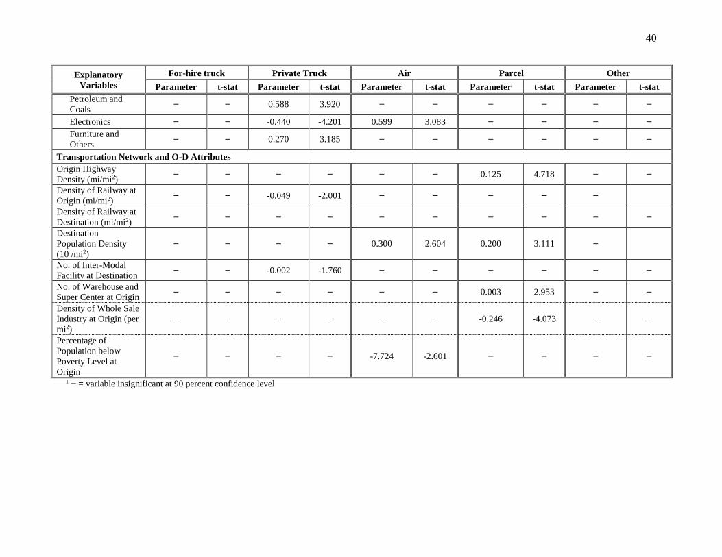
40
Explanatory
Variables
For-hire truck Private Truck Air Parcel Other
Parameter t-stat Parameter t-stat Parameter t-stat Parameter t-stat Parameter t-stat
Petroleum and
Coals − − 0.588 3.920 − − − − − −
Electronics − − -0.440 -4.201 0.599 3.083 − − − −
Furniture and
Others − − 0.270 3.185 − − − − − −
Transportation Network and O-D Attributes
Origin Highway
Density (mi/mi2) − − − − − − 0.125 4.718 − −
Density of Railway at
Origin (mi/mi2) − − -0.049 -2.001 − − − − −
Density of Railway at
Destination (mi/mi2) − − − − − − − − − −
Destination
Population Density
(10 /mi2) − − − − 0.300 2.604 0.200 3.111 −
No. of Inter-Modal
Facility at Destination − − -0.002 -1.760 − − − − − −
No. of Warehouse and
Super Center at Origin − − − − − − 0.003 2.953 − −
Density of Whole Sale
Industry at Origin (per
mi2) − − − − − − -0.246 -4.073 − −
Percentage of
Population below
Poverty Level at
Origin
− − − − -7.724 -2.601 − − − −
1 − = variable insignificant at 90 percent confidence level

41
TABLE A(ii): Copula OL (Shipment Size) Model Estimation Results
Explanatory
Variables
For-hire truck Private Truck Air Parcel Other
Parameter t-stat Parameter t-stat Parameter t-stat Parameter t-stat Parameter t-stat
Thresholds
Threshold 1 -6.283 -28.205 -5.790 -39.591 -3.896 -8.943 -0.705 -4.635 -5.631 -2.838
Threshold 2 -4.799 -24.534 -4.235 -32.314 − 1 − − − -2.982 -3.166
Threshold 3 -3.030 -17.773 -2.704 -23.065 − − − − − −
Threshold 4 -1.782 -11.143 -1.656 -15.689 − − − − − −
Threshold 5 -0.445 -2.765 -0.641 -6.495 − − − − − −
Threshold 6 0.847 4.784 -0.027 -0.261 − − − − − −
Freight Characteristics
Hazardous Material
(Base: Not
Hazardous)
Non-flammable
Liquid and Other
Hazardous
Material
0.951 2.662 − − − − − − − −
Temperature
Controlled
(Base: No)
Yes − − − − − − -0.854 -2.883 − −
SCTG Commodity
Type (Base: Wood,
Papers and Textile)
Raw Food 0.516 2.065 0.309 2.759 − − − − − −
Prepared Food and
Products 0.856 4.890 -0.275 -2.660 − − 0.553 1.999 − −
Stone & Non-
Metallic Minerals 3.131 9.910 4.447 21.648 − − − − − −
Petroleum and
Coals 1.674 6.124 0.318 2.788 − − − − − −
Chemicals − − -0.169 -1.926 − − − − − −

42
Explanatory
Variables
For-hire truck Private Truck Air Parcel Other
Parameter t-stat Parameter t-stat Parameter t-stat Parameter t-stat Parameter t-stat
Metals and
Machinery − − − − − − -0.409 -3.892 − −
Electronics -1.104 -7.976 -0.378 -2.874 -0.628 -2.226 -1.032 -10.191 − −
Furniture and
Others -0.349 -3.691 − − -0.406 -3.808 − −
Shipment Value ($)
(Base:Value >5000 )
Value ≤ 300 -3.692 -12.028 -4.348 -31.358 -1.546 -3.714 -2.489 -17.048 -5.206 -2.127
300 < Value ≤
1000 -2.934 -13.292 -3.187 -25.322 -1.166 -2.847 -0.874 -6.109 -3.390 -1.848
1000 < Value ≤
5000 -2.097 -14.993 -1.808 -16.871 -1.131 -2.812 -0.423 -2.918 − −
Transportation Network and O-D Attributes
Mean Household
Income at Origin ($)
(Base: ≥ $50,000 )
< $50,000 − − − − − − 0.347 2.235 − −
Density of Employees
in Mining Industry at
Origin (per mi2)
1.108 3.260 − − − − − − − −
Density of
Management
Company and
Enterprise at
Destination (per mi2)
− − -1.028 -3.026 − − − − − −
Density of Wholesale
Industries at
Destination (per mi2) − − − − − − -0.097 -2.632 − −
Density of Highway at
Destination (mi/mi2) − − 0.062 2.926 − − − − − −
Density of Bridges at
Destination (per mi2) -0.320 -1.963 − − − − − − − −
Origin Avg.
Temperature
(Base: Warm; > 600 F)
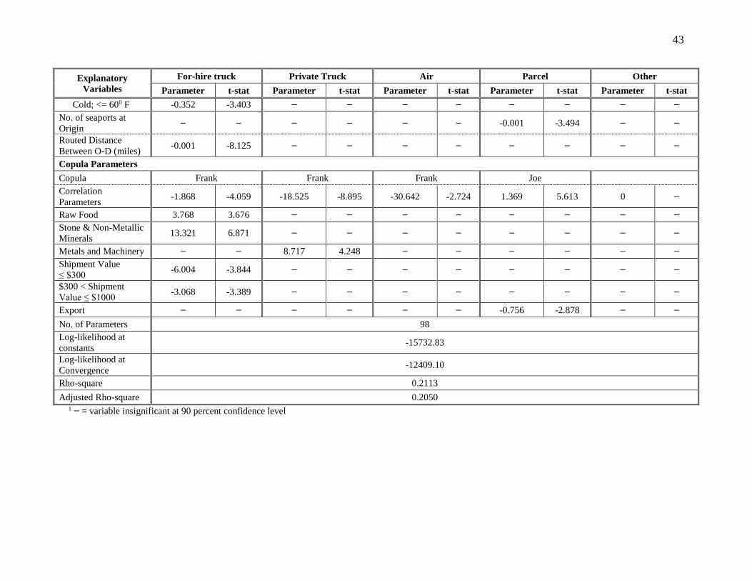
43
Explanatory
Variables
For-hire truck Private Truck Air Parcel Other
Parameter t-stat Parameter t-stat Parameter t-stat Parameter t-stat Parameter t-stat
Cold; <= 600 F -0.352 -3.403 − − − − − − − −
No. of seaports at
Origin − − − − − − -0.001 -3.494 − −
Routed Distance
Between O-D (miles) -0.001 -8.125 − − − − − − − −
Copula Parameters
Copula Frank Frank Frank Joe
Correlation
Parameters -1.868 -4.059 -18.525 -8.895 -30.642 -2.724 1.369 5.613 0 −
Raw Food 3.768 3.676 − − − − − − − −
Stone & Non-Metallic
Minerals 13.321 6.871 − − − − − − − −
Metals and Machinery − − 8.717 4.248 − − − − − −
Shipment Value
≤ $300 -6.004 -3.844 − − − − − − − −
$300 < Shipment
Value ≤ $1000 -3.068 -3.389 − − − − − − − −
Export − − − − − − -0.756 -2.878 − −
No. of Parameters 98
Log-likelihood at
constants -15732.83
Log-likelihood at
Convergence -12409.10
Rho-square 0.2113
Adjusted Rho-square 0.2050 1 − = variable insignificant at 90 percent confidence level