Pattern Recognition 61 (2017) 524–536

Contents lists available at ScienceDirect

Pattern Recognition

http://d0031-32

n CorrE-m

ymc@co

journal homepage: www.elsevier.com/locate/pr

Joint sparse principal component analysis

Shuangyan Yi a, Zhihui Lai b, Zhenyu He a,n, Yiu-ming Cheung c,d, Yang Liu c,d

a School of Computer Science, Harbin Institute of Technology Shenzhen Graduate School, Chinab The College of Computer Science and Software Engineering, Shenzhen University, Chinac Department of Computer Science, Hong Kong Baptist University, Hong Kongd The Institute of Research and Continuing Education, Hong Kong Baptist University, Hong Kong

a r t i c l e i n f o

Article history:Received 16 January 2016Received in revised form21 August 2016Accepted 22 August 2016Available online 24 August 2016

Keywords:Dimensionality reductionJoint sparseℓ2,1-norm

x.doi.org/10.1016/j.patcog.2016.08.02503/& 2016 Elsevier Ltd. All rights reserved.

esponding author.ail addresses: lai_zhi_hui@163.com (Z. Lai), zymp.hkbu.edu.hk (Y.-m. Cheung), csygliu@com

a b s t r a c t

Principal component analysis (PCA) is widely used in dimensionality reduction. A lot of variants of PCAhave been proposed to improve the robustness of the algorithm. However, the existing methods eithercannot select the useful features consistently or is still sensitive to outliers, which will depress theirperformance of classification accuracy. In this paper, a novel approach called joint sparse principalcomponent analysis (JSPCA) is proposed to jointly select useful features and enhance robustness tooutliers. In detail, JSPCA relaxes the orthogonal constraint of transformation matrix to make it have morefreedom to jointly select useful features for low-dimensional representation. JSPCA imposes joint sparseconstraints on its objective function, i.e., ℓ2,1-norm is imposed on both the loss term and the regular-ization term, to improve the algorithmic robustness. A simple yet effective optimization solution ispresented and the theoretical analyses of JSPCA are provided. The experimental results on eight data setsdemonstrate that the proposed approach is feasible and effective.

& 2016 Elsevier Ltd. All rights reserved.

1. Introduction

Dimensionality reduction is an important issue in data classi-fication. It aims to learn a transformation matrix to project thehigh-dimensional data into a low-dimensional subspace so thatthe data can be effectively classified in the low-dimensional sub-space. There are many methods for dimensionality reduction [1–5]and the classical methods are principal component analysis (PCA)[6–9] and linear discriminant analysis (LDA) [10–12]. PCA is anunsupervised method, which projects data information into anorthogonal linear space. LDA is a supervised method, which ex-tracts discriminative data information by maximizing the inter-class scatter matrix and at the same time minimizing the intra-class scatter matrix [13,14].

It is well known that PCA is an unsupervised method and theunsupervised methods are important in the practical applications[15] since labeled data are expensive to obtain [16]. However, theoriginal PCA is sensitive to outliers since its covariance matrix isderived from ℓ2-norm and ℓ2-norm is sensitive to outliers[7,17,18]. Thus, PCA fails to deal with the outliers that often appearin data sets in real-world applications. In terms of this problem,many variants of PCA [18,19,16] have been proposed to reduce the

he@hitsz.edu.cn (Z. He),p.hkbu.edu.hk (Y. Liu).

effect of outliers. One of the main strategies is to impose ℓ1-normon loss term [20,18,21,22,19]. In detail, PCA based on ℓ1-normmaximization [18] uses a greedy strategy to solve the optimizationproblem and easy to get stuck in a local solution. Robust principalcomponent analysis with non-greedy ℓ1-norm maximization(RPCA) [19] is proposed to obtain a much better solution than thatin [18]. Recently, ℓ2,1-norm has caused wide research interests[16,23,24]. Rotational invariant ℓ1-norm PCA [23] imposesℓ2,1-norm on loss term [16]. Optimal mean robust principal com-ponent analysis (OMRPCA) [16] based ℓ2,1-norm is proposed tolearn the optimal transformation matrix and optimal mean si-multaneously, which imposes ℓ2,1-norm on loss term.

Although the variants of PCA method mentioned above are ableto reduce the effect of outliers to some extent, one major dis-advantage of them is that each new feature in low-dimensionalsubspace is the linear combination of all the original features inhigh-dimensional space. Therefore, it is usually not good forclassification due to the redundant features. Besides, it is oftendifficult to interpret the new features. Actually, the interpretationof the new features is very important especially when they havephysical meanings in many applications such as gene representa-tion and face recognition. To facilitate interpretation, sparseprincipal component analysis (SPCA) [25] is proposed. However,SPCA has no ability to jointly select the useful features because theℓ1-norm is imposed on each transformation vector and ℓ1-normcannot select the consistent features. Moreover, SPCA still suffersfrom the effect of outliers because the ℓ2-norm is imposed on loss

S. Yi et al. / Pattern Recognition 61 (2017) 524–536 525

term.In this paper, we propose joint sparse principal component

analysis (JSPCA), which integrates feature selection into subspacelearning to exclude the redundant features. Specifically, JSPCAimposes joint ℓ2,1-norms on both loss term and regularizationterm. In this way, our method can discard the useless features onone hand and reduce the effect of outliers on the other hand. Themain contributions are described as follows:

(1) JSPCA relaxes the orthogonal constraint of transformationmatrix and introduces another transformation matrix to togetherrecover the original data from the subspace spanned by the se-lected features, which makes JSPCA have more freedom to jointlyselect useful features for low-dimensional representation.

(2) Unlike PCA and its existing extensions, JSPCA uses jointsparse constraints on the objective function, i.e., ℓ2,1-norm is im-posed on the loss term and the transformation matrix, to do fea-ture selection and learn the optimal transformation matrixsimultaneously.

(3) A simple yet effective optimal solution of JSPCA is provided.Furthermore, a series of theoretical analyses including con-vergence analysis, essence of JSPCA, and computational complex-ity are provided to validate the feasibility and effectiveness ofJSPCA.

The remainder of this paper is organized as follows. In Section2, we review some existing dimensionality reduction methods. InSection 3, we present the JSPCA model with an effective solution.In Section 4, we give the analyses of JSPCA in theory. In Section 5,we perform experiments and provide the observations. Finally,conclusion is drawn in Section 6.

2. Related work

In this section, we first give the basic notations and then reviewseveral variants of PCA. Suppose the given data matrix is

= [ … ] ∈ ×X x x R, , nm n

1 , where m denotes the original image spacedimensionality and n denotes the number of training samples.Without loss of generality, { } =xj j

n1 is assumed to have zero mean.

The problem of linear dimensionality reduction is to project thedata from the high-dimensional original space into a low-dimen-sional subspace. That is, we need to find a transformation matrix

= [ … ] ∈ ×A a a a R, , , dm d

1 2 with ⪡d m, where each transformationvector ak is with m loadings ( = … )k d1, 2, , . Then, the transformeddata denoted by Y can be shown as follows:

Fig. 1. Motivations of JSPCA. (a) Illustration of two transformation matrices got by JSPCmeans the non-zero loading. JSPCA can tell us that the third and the seventh features areshows more robustness to outliers than PCA.

= ∈ ( )×Y A X R . 1T d n

Notations: For the matrix A, we denote the (i,j)-th element by aij,the i-th row by Ai. In this paper, we denote = ∑ =A Ai

m i2,1 1 2

,

where Ai2means the ℓ2-norm of vector Ai and =A A Ai i T i

2.

The traditional PCA [6] based on ℓ2-norm aims to project thehigh-dimensional data onto the low-dimensional linear subspacespanned by the leading eigenvectors of the data covariance matrix.RPCA [19] based on ℓ1-norm aims to be robust to outliers by im-posing ℓ1-norm on the projected data. OMRPCA [16] based onℓ2,1-norm aims to remove optimal mean automatically and en-hance the robustness to outliers by imposing ℓ2,1-norm on the lossterm.

All of the above methods focus on operating different normssuch as ℓ2-norm, ℓ1-norm, and ℓ2,1-norm on the loss term. Al-though the above methods can get a prominent performance inmany cases, one common disadvantage of the above methods isthat each new feature is the linear combination of all the originalfeatures. To this end, the regularization term imposed by differentnorms is proposed to solve this problem. For example, based onPCA, SPCA [25] is proposed to learn a sparse projection matrix,where each new feature is the linear combination of some originalfeatures. Based on spectral regression [26], sparse subspacelearning (SSL) [27] is proposed for learning a sparse projectionmatrix, which first regress the low-dimensional projection dataand then solve the projection matrix. However, both SPCA and SSLstill cannot exclude the redundant features. Furthermore, based ongraph embedding [28], joint feature selection and subspacelearning (JFSSL) [2] is proposed to integrate the ability of featureselection into subspace learning. Although JFSSL has the ability offeature selection, it is sensitive to outliers.

3. Joint sparse principal component analysis

In this section, we first present the motivation of this work.Then, we give the objective function of the proposed method. Fi-nally, an iterative optimal solution is given for the proposed ob-jective function.

3.1. Motivation of JSPCA

As the previous statement, SPCA attempts to interpret the se-lection of features. Intuitively, we use the right subfigure in Fig. 1

A and SPCA, in which the white block means the zero loading and the gray blockthe useless features while SPCA cannot. (b) On a data set with some outliers, JSPCA

S. Yi et al. / Pattern Recognition 61 (2017) 524–536526

(a) to illustrate the learned transformation matrix by SPCA. Notethat each row of the transformation matrix corresponds to anoriginal feature while each column corresponds to a dimension-ality of the subspace. For one fixed dimensionality of the subspace,the feature with zero loading is not selected. For example, the firstfour features are not selected on the second dimensionality butthey are selected on the remaining subspace dimensionality. Be-sides, the eighth feature is not selected on the third dimensionalitybut it is selected on the remaining subspace dimensionality; thesixth feature is not selected on the sixth dimensionality but it isselected on the remaining subspace dimensionality. Since thefeature loadings across all the subspace dimensionality cannot beignorable, it still cannot tell us that which features are reallyuseless as a whole. That is, the useless feature cannot be jointlyexcluded by SPCA. Inspired by SPCA, we aim to learn a transfor-mation matrix with row-sparsity, which is shown in the left sub-figure in Fig. 1(a). In this way, the learned transformation matrixcan tell us that the third and seventh features are useless. This isthe reason that why we add ℓ2,1-norm on the transformationmatrix.

On the other hand, considering the largely appearing of outliersin real-world applications, we utilize ℓ2,1-norm on loss term toenhance the robustness to outliers. In order to test the robustnessto outliers of JSPCA, 200 points near a straight line are generatedwith 20 outliers. Then, we apply PCA and JSPCA to this data set,respectively. From Fig. 1(b), we can see that PCA is significantlyaffected while JSPCA is affected much less. This is the reason thatwhy we add ℓ2,1-norm on loss term.

3.2. Objective function of JSPCA

Considering the outliers appearing in data sets and the con-sistent selection of features, we propose the following optimiza-tion formulation:

λ( ) = − +( )

J Q P X PQ X Qarg min , arg min ,2Q P Q P

T

, ,2,1 2,1

where transformation matrix ∈ ×Q Rm d is first used to project thedata matrix X onto a low-dimensional subspace and anothertransformation matrix ∈ ×P Rm d is then used to recover the datamatrix X. Here, we relax the orthogonal constraint of transfor-mation matrix Q, introduce another transformation matrix P andadd joint ℓ2,1-norms on both loss term and regularization term. Inthis way, JSPCA can have more freedom to learn a low-dimensionalsubspace that approximates to high-dimensional data in a flexibleway. The loss term −X PQ XT

2,1is not squared and hence it en-

hances the robustness to outliers. The penalty term Q 2,1 pena-lizes all m regression coefficients corresponding to a single featureas a whole and hence our method is able to jointly select features.On the other hand, the regularization term Q 2,1 is convex and canbe easily optimized. λ ≥ 0, as a regularization parameter, is used tobalance the loss term and regularization term.

Directly solving Eq. (2) is difficult as both loss term and reg-ularization term are non-smooth [1]. Using some mathematicaltechniques for Eq. (2), we have,

( )

λ

λ

λ

λ

λ

− +

= (( − ) ( − )) + ( )

= (( − ) ( − )) + ( )

= (( ( − )) ( − )) + (( ) )

= ( − ) +3

X PQ X Q

X PQ X D X PQ X Q D Q

X PQ X D D X PQ X Q D D Q

D X PQ X D X PQ X D Q D Q

D X PQ X D Q

arg min

arg min 2tr 2 tr

arg min tr tr

arg min tr tr

arg min .

Q P

T

Q P

T T T T

Q P

T T T T T T

Q P

T T T T

Q P

TF F

,2,1 2,1

,1 2

,1 1 2 2

,1 1 2 2

,1

2

22

Hence, Eq. (2) becomes,

λ( ) = ( − ) +( )

J Q P D X PQ X D Qarg min , arg min ,4Q P Q P

TF F, ,

12

22

where

=( − )

( − )⋱ ( )

⎡

⎣

⎢⎢⎢⎢⎢⎢

⎤

⎦

⎥⎥⎥⎥⎥⎥

D

X PQ X

X PQ X

1

2

1

2

,

5

T

T

1

12

22

and

=

⋱ ( )

⎡

⎣

⎢⎢⎢⎢⎢⎢

⎤

⎦

⎥⎥⎥⎥⎥⎥

D

Q

Q

1

2

1

2

,

6

2

12

22

are two ×m m diagonal matrices. Note that ( − )X PQ XT i

( = … )i m1, 2, , means the i-th row of matrix −X PQ XT , and Qi

( = … )i m1, 2, , means the i-th row of matrix Q. When

( − ) =X PQ X 0T i2

, we let =ζ( − ) +

D ii

X PQ X1

1

2 T i2

(ζ is a very small

constant). Similarly, when =Q 0i2

, we let =ζ+

D ii

Q2

1

2 i2

. In this

way, the smaller the D ii2 is, the more important the i-th feature is.

Moreover, we can see that if ( − )X PQ XT i2and Qi

2are small, D1

and D2 are large and thus the minimization ofλ(( − ) ( − )) + ( )X PQ X D X PQ X Q D Q2tr 2 trT T T T

1 2 in Eq. (3) tends to force

( − )X PQ XT i2and Qi

2to be a very small value. After several

iterations, some ( − )X PQ XT i2and ( = … )Q i m1, 2, ,i

2may be

close to zero and thus we obtain a joint sparse Q and a small re-construction loss.

Next, let = ¯D P P1 , and = ¯−D Q Q1

1. Then, the formulation in

Eq. (4) can be rewritten as,

λ− ¯ ¯ + ¯( )¯ ¯

D X PQ D X D D Qarg min .7Q P

T

F F,1 1

2

2 12

In order to reduce the feature redundancy, we impose the ortho-

gonal constraint ¯ ¯ = ×P P IT d d for Eq. (7). Then, we have,

( )

λ( ¯ ¯) = − ¯ ¯ + ¯

¯ ¯ =

¯ ¯ ¯ ¯

× 8

J Q P D X PQ D X D D Q

P P I

arg min , arg min ,

s.t. ,

Q P Q P

T

F F

T d d

, ,1 1

2

2 12

where ¯ ∈ ×Q Rm d is first used to project the weighted data matrix

D X1 and ¯ ∈ ×P Rm d is then used to recover it.

3.3. The optimal solution

The solution of Eq. (8) is divided into the below two steps:Step 1: Given P̄ , there exists an optimal matrix ⊥̄P such that

[ ¯ ¯ ]⊥P P, is ×m m column orthogonal matrix. Then, optimizationproblem in Eq. (8) becomes,

λ− ¯ ¯ + ¯( )¯

D X PQ D X D D Qarg min .9Q

T

F F1 1

2

2 12

The first part of Eq. (9) can be rewritten as,

S. Yi et al. / Pattern Recognition 61 (2017) 524–536 527

− ¯ ¯ = − ¯ ¯

= [ ¯ ¯ ] − ¯ ¯ [ ¯ ¯ ]

= ¯ − ¯ ¯ ¯

+ ¯ − ¯ ¯ ¯

= ¯ − ¯ + ¯( )

⊥ ⊥

⊥ ⊥

⊥

D X PQ D X X D X D QP

X D P P X D QP P P

X D P X D QP P

X D P X D QP P

X D P X D Q X D P

, ,

. 10

T

FT T T

F

T T T

F

T T T

F

T T T

F

T TF

TF

1 1

2

1 1

2

1 1

2

1 1

2

1 1

2

1 12

12

Since P̄ is fixed, and ⊥̄X D PT

F12is a constant, optimization pro-

blem in Eq. (8) becomes the following optimization problem:

λ¯ − ¯ + ¯( )¯

X D P X D Q D D Qarg min .11Q

T TF F1 12

2 12

By the derivative of Eq. (11) with respect to Q̄ to be 0, we get,

λ¯ = ( + ) ¯ ( )−Q D D D D XX D D XX D P. 12T T1 2 1 1 1

11 1

Hence,

λ= ( + ) ¯ ( )−Q D XX XX D P. 13T T2

11

Step 2: Given Q̄ to compute P̄ , optimization problem in Eq. (8)becomes,

− ¯ ¯ ¯ ¯ =( )¯

×D X PQ D X P P Iarg min , s.t. .

14P

T

F

T I1 1

2 d d

The first part of Eq. (14) can be rewritten as,

− ¯ ¯

= (( − ¯ ¯ ) ( − ¯ ¯ ))

= (( − ¯ ¯ )( − ¯ ¯ ))

= ( − ¯ ¯ − ¯ ¯

+ ¯ ¯ ¯ ¯ )

= ( + ¯ ¯ ) − ( ¯ ¯) ( )

D X PQ D X

D X PQ D X D X PQ D X

X D X D QP D X PQ D X

X D X X D PQ D X X D QP D X

X D QP PQ D X

X D X X D QQ D X Q D XX D P

tr

tr

tr

tr 2tr . 15

T

FT T T

T T T T

T T T T T

T T T

T T T T T

1 1

2

1 1 1 1

1 1 1 1

1 1 1 1 1

1 1

1 1 1 1 1

Since Q̄ is given, Eq. (14) becomes,

( ¯ ¯) ¯ ¯ =( )¯

×Q D XX D P P P Iarg min tr , s.t. .16P

T T T d d1 1

On the other hand, optimization problem in Eq. (14) is equal to,

− ¯ ¯ ¯ ¯ =( )¯

×X D X D QP P P Iarg min , s.t. .17P

T T T

F

T d d1 1

2

The update of P̄ of minimizing Eq. (17) with the constraint of¯ ¯ = ×P P I

T d d means that P̄ is orthogonal in the columns. In order tocompute P̄ , we introduce the following lemma [25].

Lemma 1. Let ×Zn m and ×Vn d be two matrices. Consider the con-strained minimization problem,

− =( )

×Z VP s t P P Iarg min , . . .18P

T T d d2

Suppose the SVD of Z VT is EDUT , then the optimal solution is =P EUT .

According to Lemma 1, we have =Z V DT1

¯XX D QT1 . Let the

SVD of ¯ =D XX D Q EDUT T1 1 , we have,

¯ = ( )P EU . 19T

Thus,

= ( )−

P D EU . 20T1

1

In fact, before we compute Q̄ in Eq. (12), we need to compute theinput of matrix P̄ , D1 and D2, which cannot be obtained directly.Therefore, we need to compute them in the designed iterativealgorithm. Once P̄ , Q̄ , D1 and D2 are obtained, we can obtain P andQ according to Eqs. (20) and (13). According to the obtained P andQ, we get the new D1 and D2. Iterating the above procedures willgive the local optimal solutions of the algorithm. Algorithm 1 givesthe details.

4. Discussion and analysis

In this section, we will further give the theoretical analysis ofthe proposed method, which includes convergence analysis, es-sence of the optimization algorithm, connection to weighted PCAand computational complexity analysis.

4.1. Convergence analysis

Before giving the proof of convergence of the proposed optimalalgorithm, we need to give the following lemma [29].

Lemma 2. For any nonzero vectors ∈p q R, c , the following resultholds:

− ≤ −( )

pp

qq

q

q2 2.

21222

22

22

2

Based on Lemma 2, we give the following proposed theorem.

Theorem 1. Given all the variables in Eq. (2) except for P, Q, theoptimal problem in Eq. (2) will monotonically decrease the objectivefunction value in each iteration and converge to the local optimumsolution.

Proof. For simplicity, we denote the objective function in Eq. (2)as ( ) = ( )J Q P J Q P D D, , , ,1 2 , suppose for the −t 1-th iteration, weobtain ( − )P t 1 , ( − )Q t 1 , ( − )D t

11 and ( − )D t

21 . From Eq. (13), we can find that,

( ) ≤ ( ) ( )( ) ( − ) ( − ) ( − ) ( − ) ( − ) ( − ) ( − )J Q P D D J Q P D D, , , , , , . 22t t t t t t t t11

12

1 1 11

12

1

Since the SVD gives the optimal ( )P t that further decreases theobjective value, we have,

( ) ≤ ( ) ( )( ) ( ) ( − ) ( − ) ( − ) ( − ) ( − ) ( − )J Q P D D J Q P D D, , , , , , . 23t t t t t t t t1

12

1 1 11

12

1

Once the optimal ( )P t and ( )Q t are obtained, we have,

λ

λ

(( − ) ( − )) + ( )

≤ (( − ) ( − ))

+ ( ) ( )

( ) ( ) ( − ) ( ) ( ) ( ) ( − ) ( )

( − ) ( − ) ( − ) ( − ) ( − )

( − ) ( − ) ( − )

X P Q X D X P Q X Q D Q

X P Q X D X P Q X

Q D Q

tr tr

tr

tr . 24

t t T T t t t T t T t t

t t T T t t t T

t T t t

11

21

1 11

1 1 1

12

1 1

That is,

∑ ∑

∑ ∑

λ

λ

−

−+

≤−

−+

( )

=

( ) ( )

( − ) ( − )=

( )

( − )

=

( − ) ( − )

( − ) ( − )=

( − )

( − )

⎛

⎝⎜⎜⎜

⎞

⎠⎟⎟⎟

⎛

⎝⎜⎜⎜

⎞

⎠⎟⎟⎟

⎛

⎝⎜⎜⎜

⎞

⎠⎟⎟⎟

⎛

⎝⎜⎜⎜

⎞

⎠⎟⎟⎟

X P Q X

X P Q X

Q

Q

X P Q X

X P Q X

Q

Q

tr tr

tr tr .

25

i

mi

ti

t T

it

it T

i

mi

t

it

i

mi

ti

t T

it

it T

i

mi

t

it

1

2

2

1 12

1

2

2

12

1

1 12

2

1 12

1

12

2

12

On one hand, according to Lemma 2, we have,

Inp

12

e3

Fig. 2. Visualization of some original data sets and their corresponding corruptions, where the original images from four data sets are shown in the first row and thecorresponding corrupted images are shown in the second row. Specifically, each image of AR and Yale data sets is corrupted by 10�10 block occlusions while ORL andCOIL20 data sets are corrupted by 10% salt & pepper noises.

S. Yi et al. / Pattern Recognition 61 (2017) 524–536528

− −−

−

≤ − −−

− ( )

( ) ( )( ) ( )

( − ) ( − )

( − ) ( − )( − ) ( − )

( − ) ( − )

X P Q XX P Q X

X P Q X

X P Q XX P Q X

X P Q X.

26

it

it T i

ti

t T

it

it T

it

it T i

ti

t T

it

it T

22

2

1 12

1 12

1 12

2

1 12

Using the matrix calculus for Eq. (26), we have the formulation asfollows:

∑

∑

− −−

−

≤ − −−

−( )

=

( ) ( )( ) ( )

( − ) ( − )

=

( − ) ( − )( − ) ( − )

( − ) ( − )

⎛

⎝⎜⎜⎜

⎞

⎠⎟⎟⎟

⎛

⎝⎜⎜⎜

⎞

⎠⎟⎟⎟

X P Q XX P Q X

X P Q X

X P Q XX P Q X

X P Q X.

27

i

m

it

it T i

ti

t T

it

it T

i

m

it

it T i

ti

t T

it

it T

12

2

2

1 12

1

1 12

1 12

2

1 12

On the other hand, according to Lemma 2, we have,

− ≤ −( )

( )( )

( − )( − )

( − )

( − )Q

Q

QQ

Q

Q,

28i

t it

it i

t it

it2

2

2

12

12

12

2

12

Similarly, using the matrix calculus for Eq. (28), we have the for-mulation as follows:

∑ ∑− ≤ −

( )=

( )( )

( − )=

( − )( − )

( − )

⎛

⎝⎜⎜⎜

⎞

⎠⎟⎟⎟

⎛

⎝⎜⎜⎜

⎞

⎠⎟⎟⎟Q

Q

QQ

Q

Q.

29i

m

it i

t

it

i

m

it i

t

it

12

2

2

12 1

12

12

2

12

By combining Eqs. (25) and (27) with Eq. (29), we have,

λ

λ

( ) = − +

≤ − +

= ( ) ( )

( ) ( ) ( − ) ( − ) ( ) ( ) ( )

( − ) ( − ) ( − )

( − ) ( − ) ( − ) ( − )

J Q P D D X P Q X Q

X P Q X Q

J Q P D D

, , ,

, , , . 30

t t t t t t T t

t t T t

t t t t

11

21

21 21

1 121

121

1 11

12

1

That is,

( ) = ( ) ≤ ( )

= ( ) ( )

( ) ( ) ( ) ( ) ( ) ( ) ( − ) ( − ) ( − ) ( − )

( − ) ( − )

J Q P J Q P D D J Q P D D

J Q P

, , , , , , ,

, . 31

t t t t t t t t t t

t t

1 21 1

11

21

1 1

Table 1Classification performance (average classification accuracy with standard deviation) on

Data sets Baseline PCA RPCA OM

ORL/3 0.745070.0314 0.743270.0288 0.801670.0201 0.8ORL/5 0.850070.0281 0.863070.0265 0.863570.0321 0.8ORL/7 0.923370.0292 0.904270.0297 0.935670.0245 0.9

AR/8 0.721870.0105 0.701770.0101 0.726270.0135 0.7AR/13 0.733370.0088 0.742370.0197 0.739670.0153 0.7AR/18 0.873370.0112 0.850770.0117 0.850870.0091 0.8

Yale/22 0.698470.0118 0.718870.0026 0.687370.0050 0.7Yale/27 0.745770.0048 0.761570.0102 0.734270.0086 0.7Yale/32 0.783170.0149 0.826670.1068 0.752070.0164 0.7

Therefore, the optimization problem in Eq. (2) can converge to thelocal optimum solution. □

Algorithm 1. JSPCA algorithm

the fa

RPCA

070771073507

308742376127

172765277807

ut: Training sample set X, parameter λ, and dimensionalityd.

: Initialize = ×D Im m1 , = ×D Im m

2 and random ¯ ×P

m d.: while not converge do2.1: Compute Q̄ according to Eq. (12)2.2: Compute Q according to Eq. (13)2.3: Compute P̄ according to Eq. (19)2.4: Compute P according to Eq. (20)2.5: Compute D1 according to Eq. (5)2.6: Compute D2 according to Eq. (6)nd while: Normalize each column vectors of Q to be identity vectors.tput: Transformation matrix Q.

Ou

4.2. Essence of JSPCA

4.2.1. The intrinsic relationship between P and QIn order to explore the essence of P and Q in Eq. (2), we need to

explore the essence of P̄ and Q̄ in Eq. (8).Substituting Eq. (12) into Eq. (16), we get the following opti-

mization problem:

λ( ¯ ( + )

¯) ¯ ¯ = ( )

¯

−

×

P D XX D D D D D XX D D

XX D P P P I

arg min tr

, s.t. . 32

P

T T T

T T d d

1 1 1 2 1 1 11

1

1

It is clear that the optimal solution P̄ is the standard eigende-composition of the following eigen equation:

λ Σ( + ) ¯ = ¯ ( )−D XX D D D D D XX D D XX D P P , 33T T T1 1 1 2 1 1 1

11 1

where Σ is the eigenvalue matrix. Therefore, P̄ contains the ei-genvectors corresponding to the larger eigenvalues of Eq. (33).If P̄ contains all the eigenvectors of Eq. (33), since Eqs. (12)and (33) can be rewritten as Σ¯ = ¯D XX D Q PT

1 1 . Furthermore,

cial data sets with different training samples.

SPCA SSL JSPCA

0.0148 0.764170.0289 0.730070.0268 0.809570.01760.0224 0.864070.0227 0.869070.0201 0.905070.02360.0257 0.919870.0211 0.921770.0173 0.939270.0241

0.0063 0.760870.0152 0.763670.0215 0.770070.01220.0138 0.809070.0267 0.816970.0075 0.820670.01520.0056 0.868270.0200 0.874570.0089 0.878070.0172

0.0078 0.656070.0313 0.751870.0187 0.770070.00860.0114 0.708170.0222 0.773670.0103 0.813570.00850.0130 0.736070.0702 0.795870.0130 0.8455 70.1085

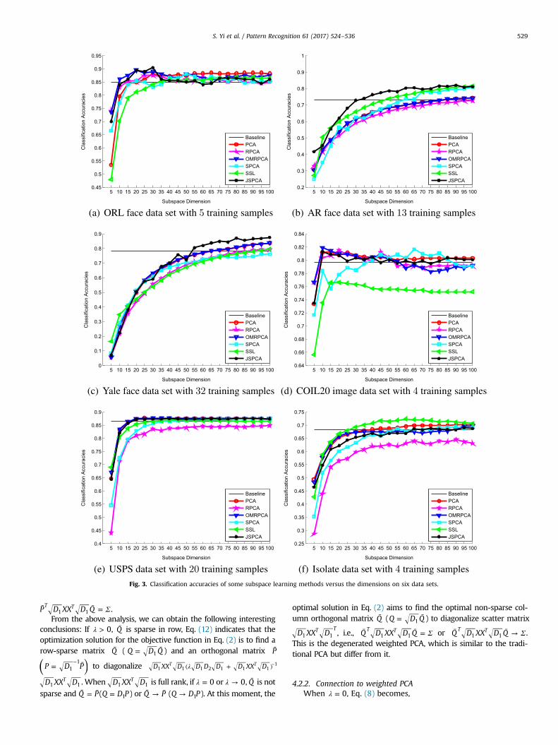
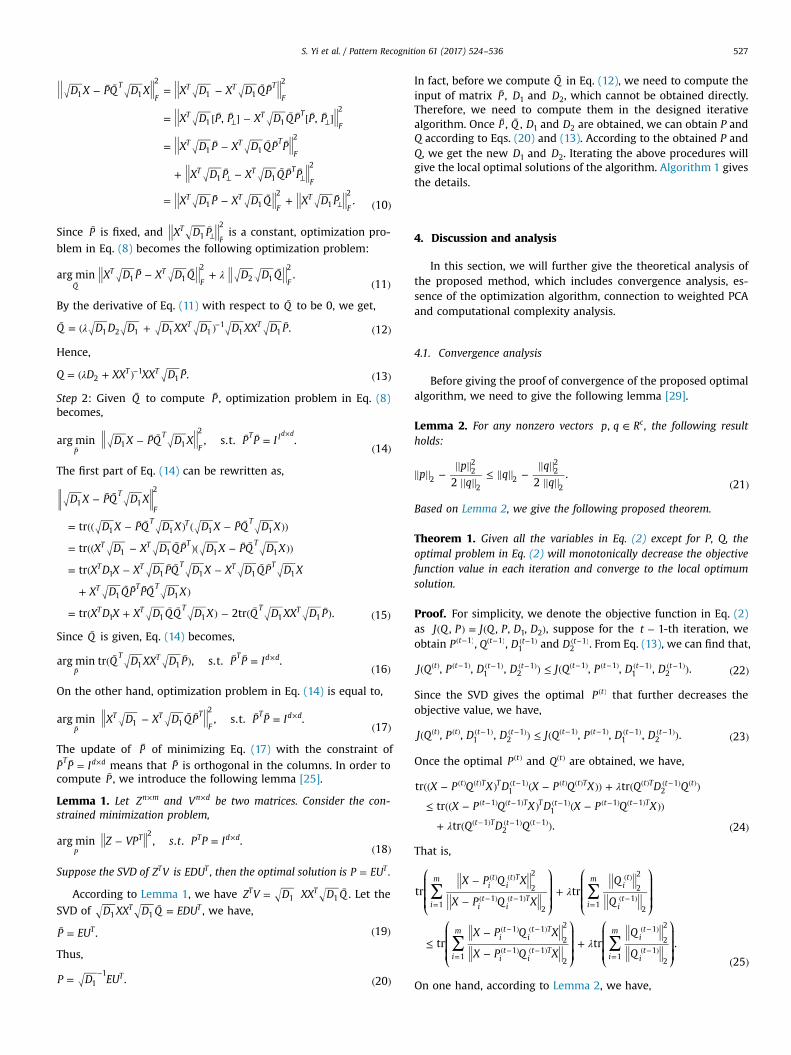
Fig. 3. Classification accuracies of some subspace learning methods versus the dimensions on six data sets.

S. Yi et al. / Pattern Recognition 61 (2017) 524–536 529

Σ¯ ¯ =P D XX D QT T

1 1 .From the above analysis, we can obtain the following interesting

conclusions: If λ > 0, Q̄ is sparse in row, Eq. (12) indicates that theoptimization solution for the objective function in Eq. (2) is to find arow-sparse matrix Q̄ ( = ¯Q D Q1 ) and an orthogonal matrix P̄

( )= ¯−P D P1

1to diagonalize λ( + )−D XX D D D D D XX DT T

1 1 1 2 1 1 11

D XX DT1 1 . When D XX DT

1 1 is full rank, if λ = 0 or λ → 0, Q̄ is not

sparse and ¯ = ¯Q P( =Q D P1 ) or ¯ → ¯Q P ( →Q D P1 ). At this moment, the

optimal solution in Eq. (2) aims to find the optimal non-sparse col-umn orthogonal matrix Q̄ ( = ¯Q D Q1 ) to diagonalize scatter matrix

D XX DT T1 1 , i.e., Σ¯ ¯ =Q D XX D Q

T T1 1 or Σ¯ ¯ →Q D XX D Q

T T1 1 .

This is the degenerated weighted PCA, which is similar to the tradi-tional PCA but differ from it.

4.2.2. Connection to weighted PCAWhen λ = 0, Eq. (8) becomes,

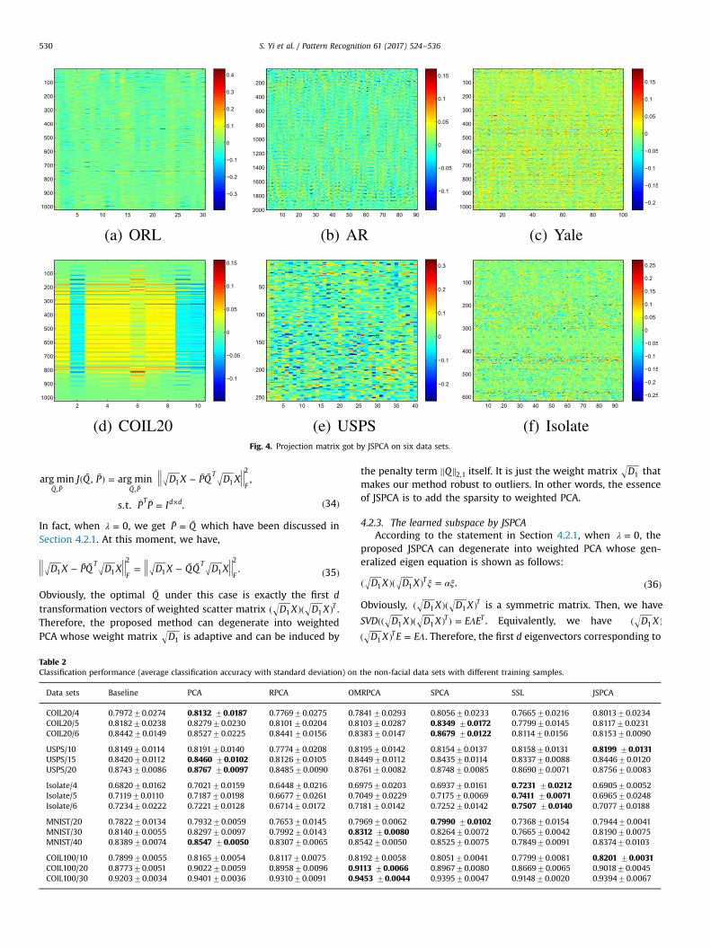
Fig. 4. Projection matrix got by JSPCA on six data sets.

S. Yi et al. / Pattern Recognition 61 (2017) 524–536530

( ¯ ¯) = − ¯ ¯

¯ ¯ = ( )

¯ ¯ ¯ ¯

×

J Q P D X PQ D X

P P I

arg min , arg min ,

s.t. . 34

Q P Q P

T

F

T d d

, ,1 1

2

In fact, when λ = 0, we get ¯ = ¯P Q which have been discussed inSection 4.2.1. At this moment, we have,

− ¯ ¯ = − ¯ ¯( )D X PQ D X D X QQ D X . 35

T

F

T

F1 1

2

1 1

2

Obviously, the optimal Q̄ under this case is exactly the first dtransformation vectors of weighted scatter matrix ( )( )D X D X T

1 1 .Therefore, the proposed method can degenerate into weightedPCA whose weight matrix D1 is adaptive and can be induced by

Table 2Classification performance (average classification accuracy with standard deviation) on

Data sets Baseline PCA RPCA OM

COIL20/4 0.797270.0274 0.8132 70.0187 0.776970.0275 0.7COIL20/5 0.818270.0238 0.827970.0230 0.810170.0204 0.8COIL20/6 0.844270.0149 0.852770.0225 0.844170.0156 0.8

USPS/10 0.814970.0114 0.819170.0140 0.777470.0208 0.8USPS/15 0.842070.0112 0.8460 70.0102 0.812670.0105 0.8USPS/20 0.874370.0086 0.8767 70.0097 0.848570.0090 0.8

Isolate/4 0.682070.0162 0.702170.0159 0.644870.0216 0.6Isolate/5 0.711970.0110 0.718770.0198 0.667770.0261 0.7Isolate/6 0.723470.0222 0.722170.0128 0.671470.0172 0.7

MNIST/20 0.782270.0134 0.793270.0059 0.765370.0145 0.7MNIST/30 0.814070.0055 0.829770.0097 0.799270.0143 0.8MNIST/40 0.838970.0074 0.8547 70.0050 0.830770.0065 0.8

COIL100/10 0.789970.0055 0.816570.0054 0.811770.0075 0.8COIL100/20 0.877370.0051 0.902270.0059 0.895870.0096 0.9COIL100/30 0.920370.0034 0.940170.0036 0.931070.0091 0.9

the penalty term Q 2,1 itself. It is just the weight matrix D1 thatmakes our method robust to outliers. In other words, the essenceof JSPCA is to add the sparsity to weighted PCA.

4.2.3. The learned subspace by JSPCAAccording to the statement in Section 4.2.1, when λ = 0, the

proposed JSPCA can degenerate into weighted PCA whose gen-eralized eigen equation is shown as follows:

ξ αξ( )( ) = ( )D X D X . 36T1 1

Obviously, ( )( )D X D X T1 1 is a symmetric matrix. Then, we have

Λ(( )( ) ) =SVD D X D X E ET T1 1 . Equivalently, we have ( )D X1

Λ( ) =D X E ET1 . Therefore, the first d eigenvectors corresponding to

the non-facial data sets with different training samples.

RPCA SPCA SSL JSPCA

84170.0293 0.805670.0233 0.766570.0216 0.801370.023410370.0287 0.8349 70.0172 0.779970.0145 0.811770.023138370.0147 0.8679 70.0122 0.811470.0156 0.815370.0090

19570.0142 0.815470.0137 0.815870.0131 0.8199 70.013144970.0112 0.843570.0114 0.833770.0088 0.844670.012076170.0082 0.874870.0085 0.869070.0071 0.875670.0083

97570.0203 0.693770.0161 0.7231 70.0212 0.690570.005204970.0229 0.717570.0069 0.7411 70.0071 0.696570.024818170.0142 0.725270.0142 0.7507 70.0140 0.707770.0188

96970.0062 0.7990 70.0102 0.736870.0154 0.794470.0041312 70.0080 0.826470.0072 0.766570.0042 0.819070.007554270.0050 0.852570.0075 0.784970.0091 0.837470.0103

19270.0058 0.805170.0041 0.779970.0081 0.8201 70.0031113 70.0066 0.896770.0080 0.866970.0065 0.901870.0045453 70.0044 0.939570.0047 0.914870.0020 0.939470.0067

Table 3Classification performance (average classification accuracy with standard deviation) on eight corrupted data sets with different training samples.

Data sets PCA RPCA OMRPCA SPCA SSL JSPCA

ORL/5 0.840070.0200 0.820070.0199 0.845070.0128 0.840070.0209 0.688070.0261 0.8600 70.0145AR/13 0.614770.0063 0.595570.0195 0.614770.0088 0.672470.0067 0.686370.0173 0.6904 70.0192Yale/32 0.694570.0288 0.659470.0291 0.694570.0168 0.706270.0200 0.282570.0268 0.7204 70.0112COIL20/4 0.736870.0116 0.746370.0191 0.736070.0198 0.739070.0109 0.659470.0168 0.7507 70.0092USPS/20 0.852570.0104 0.795670.0197 0.8528 70.0197 0.848270.0117 0.804970.0103 0.845470.0147Isolate/4 0.6599 70.0134 0.577170.0238 0.659970.0182 0.655270.0309 0.617670.0185 0.646370.0179MNIST/40 0.840170.0074 0.779370.0114 0.8416 70.0091 0.840770.0077 0.739870.0181 0.808470.0075COIL100/10 0.665270.0102 0.655870.0055 0.676670.0093 0.688570.0087 0.527470.0125 0.7976 70.0093

Fig. 5. Classification accuracies of some subspace learning methods versus the dimensions on six corrupted data sets.

S. Yi et al. / Pattern Recognition 61 (2017) 524–536 531

S. Yi et al. / Pattern Recognition 61 (2017) 524–536532

the increasing ordered eigenvalues of the eigenfunction of Eq. (36)are exactly the first d columns of E. Φ = { }span E is the subspacespanned by eigenvectors of the generalized eigenfunction (36) ofweighted PCA.

In the following, we discuss the relationship between Q got byJSPCA and the eigenvectors of Eq. (36).

Substituting Eq. (19) into Eq. (13), we have,

λ= ( + ) ( )−Q D XX XX D EU . 37T T T2

11

Note that when λ → 0 and XXT is full rank, we have →Q D EUT1 .

Denote our sparse subspace as Ω. Then, Ω = { } →span Q spanΦ{ } = { } =D E span E1 . When =D I1 , Eq. (36) becomes ξ αξ=XXT ,

which is the eigen equation of traditional PCA. The D1 in JSPCA isnot usually I.

4.3. Computational complexity analysis

The main computational complexity of JSPCA have two steps ineach iteration, the first step is to compute λ= ( + ) ¯−Q D XX XX D PT T

21

1

with ( )O m3 . The second step is to compute the SVD of¯ =D XX D Q EDUT T

1 1 , whose computational complexity is also

( )O m3 at most. Therefore, the computational complexity of oneiteration will be up to ( )O m3 . If the algorithm needs t iteration steps,then the total computational complexity is in the order of ( )O tm3 .

5. Experiments

To evaluate JSPCA, we compare it with the traditional PCA andits variants including PCA [6], RPCA [19], OMRPCA [16], SPCA [25],and SSL [27]. In order to compare the dimensionality reductionperformance of different methods objectively and persuasively, wetest these methods on each data set using the nearest neighbor(NN) classifier to obtain the classification accuracy.

Additionally, in order to test the robustness to outliers of JSPCA,we simulate the following two levels of corruptions:

(1) Block occlusions: The block occlusions are randomly addedto different locations in each image with block size of 10�10.

(2) Random pixel corruptions: The pixels are randomly chosenfrom each image and corrupted by salt & pepper noises. The rate ofcorrupted pixels is 10%.

Our experiments are divided into two groups: One is the ex-periments on the original data sets; the other is the experimentson the corrupted data sets. The so-called corrupted data sets areconstructed in this way: we add the block occlusions on AR andYale (Extended Yale B) data sets; we add random pixel corruptions

Fig. 6. Parameter selecti

on ORL, COIL20, USPS, Isolate, MNIST, and COIL100 data sets. Fig. 2shows some original images in the first row and the correspondingcorrupted images in the second row.

5.1. Data sets

The ORL face data set, including frontal views of faces withdifferent facial expressions and lighting conditions, contains 40individuals and each individual contains 10 face images. Here, weresize each image to 56�46 pixels.

The AR face data set [30,31], including frontal views of faceswith different facial expressions, lighting conditions and occlu-sions (glasses and scarf), contains 120 individuals in which eachindividual contains 26 images. Here, we resize each image to50�40 pixels.

The Yale face data set [32,33] contains 2414 frontal face imagesof 38 individuals [32] under different lighting conditions. Eachindividual contains about 64 images and half of the images arecorrupted by shadows or reflection. Here, each image is croppedand resized to 50�40 pixels.

The COIL20 image data set [34] contains 20 individuals inwhich each individual contains 72 images and each image is takenat pose intervals of 5°. Here, each image is converted to a gray-scale image of 32�32 pixels.

The USPS data set [35] contains totally 9298 digit images from0 to 9, each of which is of size 16�16 pixels, with 256 gray levelsper pixel.

The used Isolate data set [36] contains totally 150 speakerswho spoke the name of each letter of the alphabet twice. Thespeakers are grouped into sets of 30 speakers each and are re-ferred to as Isolate1 through isolate5. Here, we refer Isolate1 asthe used Isolate data set where the dimensionality is 617 andsize is 1560.

The used MNIST data set (http://www.cad.zju.edu.cn/home/dengcai/Data/MLData.html) contains totally 4000 digit imagesfrom 0 to 9, each of which is of size 28�28 pixels, with 784 graylevels per pixel.

The COIL100 data set (http://www.cad.zju.edu.cn/home/dengcai/Data/MLData.html) contains 100 individuals in which eachindividual contains 72 images and each image is taken at poseintervals of 5°. Here, each image is converted to a gray-scale imageof 32�32 pixels.

5.2. Experiments on the original data sets

5.2.1. Experiments on the facial data setsOn the ORL data set, we randomly select 3, 5, and 7 samples

on on six data sets.

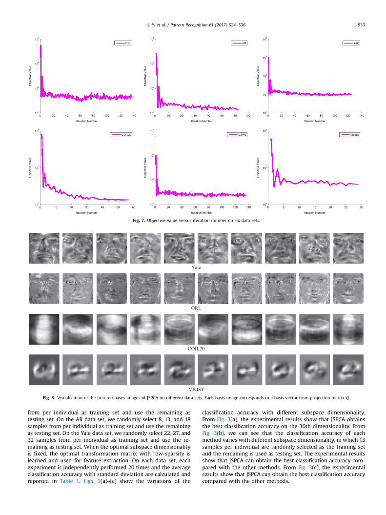
Fig. 7. Objective value versus iteration number on six data sets.

Fig. 8. Visualization of the first ten bases images of JSPCA on different data sets. Each basis image corresponds to a basis vector from projection matrix Q.

S. Yi et al. / Pattern Recognition 61 (2017) 524–536 533

from per individual as training set and use the remaining astesting set. On the AR data set, we randomly select 8, 13, and 18samples from per individual as training set and use the remainingas testing set. On the Yale data set, we randomly select 22, 27, and32 samples from per individual as training set and use the re-maining as testing set. When the optimal subspace dimensionalityis fixed, the optimal transformation matrix with row-sparsity islearned and used for feature extraction. On each data set, eachexperiment is independently performed 20 times and the averageclassification accuracy with standard deviation are calculated andreported in Table 1. Figs. 3(a)–(c) show the variations of the

classification accuracy with different subspace dimensionality.From Fig. 3(a), the experimental results show that JSPCA obtainsthe best classification accuracy on the 30th dimensionality. FromFig. 3(b), we can see that the classification accuracy of eachmethod varies with different subspace dimensionality, in which 13samples per individual are randomly selected as the training setand the remaining is used as testing set. The experimental resultsshow that JSPCA can obtain the best classification accuracy com-pared with the other methods. From Fig. 3(c), the experimentalresults show that JSPCA can obtain the best classification accuracycompared with the other methods.

Table 4Reconstruction error comparisons of six PCA methods on the training samples ofCOIL20 data set using different dimensions.

Methods 10 20 30 40 50 60

PCA ×1.8442 105 ×1.4265 105 1.2485× 105

1.0937× 105

9.9127

×104

9.1058

×104

RPCA 2.0528 × 105 1.5905 × 105 1.3409× 105

1.2248× 105

1.0911× 105

9.6751

×104

OMRPCA 1.9450 × 105 1.4503 × 105 1.2750× 105

1.1498× 105

1.0348× 105

9.6341

×104

SPCA 4.5913 × 105 4.4378 × 105 4.3226× 105

4.1953× 105

4.1361× 105

4.1428× 105

SSL 4.5851 × 105 4.5392 × 105 4.5264× 105

4.5236× 105

4.5375× 105

4.5386× 105

JSPCA 2.4480 × 105 2.0410 × 105 1.8658× 105

1.8138× 105

1.7298× 105

1.6691× 105

Table 5Reconstruction error comparisons of six PCA methods on the training samples ofAR data set using different dimensions.

Methods 50 60 70 80 90 100

PCA 2.3924 ×106

2.2343 ×106

2.0741 ×106

1.9710 ×105

1.9196 ×106

1.8540 ×106

RPCA 2.5253 ×106

2.4010 ×106

2.2146 ×106

2.1242 ×106

2.1115 ×106

1.9867 ×106

OMRPCA 2.3622 ×106

2.2078 ×106

2.0536 ×106

1.9511 ×106

1.8988 ×106

1.8348 ×106

SPCA 8.6334 ×106

8.3803 ×106

8.1822 ×106

7.9305 ×106

7.7310 ×106

7.4437 ×106

SSL 9.8424 ×106

9.8421 ×106

9.8418 ×106

9.8413 ×106

9.8412 ×106

9.8410 ×106

JSPCA 3.5027 ×106

3.4986 ×106

3.5156 ×106

3.5730 ×106

3.5860 ×106

3.6118 ×106

S. Yi et al. / Pattern Recognition 61 (2017) 524–536534

In fact, it is difficult to get high classification accuracy on thesefacial data sets due to the different variations such as occlusions inAR, illuminations in Yale and pose variations in ORL. However, theexperimental results from Table 1 and Figs. 3(a)–(c) show thatJSPCA can obtain the better classification accuracy than othercompared methods. This is because JSPCA uses the ℓ2,1-norm toconstrain the projection matrix. In this way, the projection matrixwith row-sparsity can indicate the importance degree of the fea-tures. On the other hand, JSPCA uses the ℓ2,1-norm to constrain theloss term, and the loss term can be gradually trending to thesmaller value by D1 (see Eq. (5)). Therefore, JSPCA is robust to thenegative influence of the data set with complicated variations tosome extent. The obtained projection matrix is intuitively dis-played in the first row of Fig. 4.

5.2.2. Experiments on the non-facial data setsOn the COIL20 data set, we randomly select 4, 5, and 6 samples

from per subject as training set and use the remaining as testingset. On the USPS data set, we randomly select 10, 15, and 20samples from per subject as training set and use the remaining astesting set. On the Isolate data set, we randomly select 4, 5, and6 samples from per subject as training set and use the remainingas testing set. When the optimal subspace dimensionality is fixed,the optimal transformation matrix with row-sparsity is learnedand used for feature extraction. Each experiment is independentlyperformed 20 times and the average classification accuracy withstandard deviation are calculated and reported in Table 2. Figs. 3(d)–(f) show the variations of the classification accuracy with dif-ferent subspace dimensionality. From Fig. 3(d), the experimentalresults show that JSPCA obtains the approximated classification

accuracy with the other compared methods. From Fig. 3(e), theexperimental results show that JSPCA obtains the approximatedclassification accuracy with the other compared methods. FromFig. 3(f), the experimental results show that SSL obtains the bestclassification accuracy and JSPCA gets an approximated result toSSL. To sum up, from Table 2 and Figs. 3(d)–(f), we can see that theexperimental results obtained by JSPCA approximate to that ofother compared methods. The obtained projection matrix on somenon-facial data sets are intuitively displayed in the second row ofFig. 4.

5.3. Experiments on the corrupted data sets

Table 3 lists the experimental results with the optimal subspacedimensionality on the eight corrupted data sets where ORL facedata set uses 5 samples per individual as the training set, AR facedata set uses 13 samples per individual as the training set, Yaleface data set uses 32 samples per individual as the training set,COIL20 data set uses 4 samples per subject as the training set,USPS data set uses 20 samples per subject as the training set, andIsolate data set uses 4 samples per subject as the training set. Fig. 5shows the variation of the classification accuracy of each methodversus the different dimensionality on the corrupted data set.Compared with Fig. 3, we can see that JSPCA not only outperformsthe other compared methods on the three original facial data sets,but also outperforms them on the corrupted non-facial data sets.Moreover, JSPCA approximates the OMRPCA and SPCA on thecorrupted non-facial data sets.

Although JSPCA performs well on the corrupted data setscompared to the other methods, JSPCA suffers from the influenceof random corruptions inevitably due to its ability of feature se-lection. Therefore, JSPCA is more robust to the slight complicatedvariations in the original data sets rather than the added randomcorruptions on the original data sets.

5.4. Parameter settings

For the proposed optimization problem in Eq. (9), there are oneparameter, i.e., λ. We first use the grid search method to search theoptimal parameter λ in the scope of [ ]−10 , 106 6 , and then narrowthe search scope to be [ ]0, 6.4 . As can be seen, Fig. 6 shows theinfluence of different settings of λ on six data sets. On ORL data set,the impact is small and the more robust parameter range is[ ]0.05, 0.8 . On AR data set, the best classification performance canbe got when λ = 0.05 and the more robust parameter range is[ ]0, 0.8 . On Yale data set, the best classification performance is gotwhen λ = 0.05 and the more robust parameter range is [ ]0, 0.8 . OnCOIL20 data set, the best classification performance corresponds toλ = 0.2 and the more robust parameter range is [ ]0, 0.4 . On USPSand Isolate data sets, the best classification performance corres-ponds to λ = 0.05. We can see that JSPCA can achieve betterclassification performance over a reasonable range of λ, and isrobust to the different settings of λ as long as the values are in thereasonable range. Overall, the better classification performance isusually achieved when λ is close to 0.05. However, when λ → 0,the classification accuracy will decrease. This indicates that theregularization parameter λ is also important for JSPCA to achieveits best performance.

5.5. Observations

Based on the experimental results shown in the above sub-sections, we have the following observations and analyses:

(1) Sparsity of JSPCA: The regularization term of JSPCA is im-posed by ℓ2,1-norm, which is defined to encourage the rows of the

S. Yi et al. / Pattern Recognition 61 (2017) 524–536 535

projection matrix to be zero. Hence, the projection matrix Q can beused to indicate the significance of the features, which are in-tuitively displayed in Fig. 4. This shows that the regularizationterm of JSPCA imposed by ℓ2,1-norm can exclude the redundantfeatures and improve the classification performance.

(2) Convergence of JSPCA: Theoretical analysis in Section 4.1indicates that JSPCA is convergent. Fig. 7 shows the convergencecurves of JSPCA on six data sets where the max iteration number is140.

(3) Bases images of JSPCA: To further observe JSPCA, we give thebases images of JSPCA on four data sets (see Fig. 8). Specifically, forthe facial data sets, the selected features are those importantfeatures such as eyes, nose, mouth, and facial contour. For thosenon-facial data sets, the selected features are the different con-tours of different subjects.

5.6. Discussion

In this paper, JSPCA is proposed to find representative featuresfrom the original high-dimensional space. The found re-presentative features have been used for classification tasks. Al-though JSPCA outperforms the other PCA methods in most ofclassification experiments, a series of PCA methods includingJSPCA achieve the low classification accuracy overall. This is be-cause these PCA methods do not use class labels to extract dis-criminative features. Any dimensionality reduction method with-out using class labels does not always extract effective features forclassification. In the future, our method would be extended to thesupervised method to solve the skewed/imbalanced classificationproblem.

In order to further rich the proposed method, the found re-presentative features are also used for reconstruction experimentsas shown in Tables 4 and 5.

From these two tables, we can see that JSPCA achieves a betterreconstruction than SPCA and SSL. This is because JSPCA is able toselect the effective features for reconstruction while SPCA and SSLare not. Moreover, JSPCA has a worse reconstruction than PCA,RPCA, and OMRPCA. This is a matter of course because JSPCA in-evitably suffers from the loss of some information.

6. Conclusion

In this paper, JSPCA is designed by relaxing the orthogonalconstraint of transformation matrix Q, introducing another trans-formation matrix P and imposing joint ℓ2,1-norms on both lossterm and regularization term. The proposed method has morefreedom to jointly select the useful features for a low-dimensionalrepresentation and is robust to outliers. A simple yet effective al-gorithm is designed for the optimization problem. A series oftheoretical analyses are discussed which reveal some intrinsicqualities of the proposed method. In essence, JSPCA is theweighted PCA with sparsity. Experiments on eight benchmark datasets show the feasibility and effectiveness of JSPCA compared tothe original PCA and its variants.

Acknowledgments

This study was supported by the Shenzhen Research Council(Grant nos. JSGG20150331152017052, JCYJ20140819154343378,JCYJ20160406161948211), partially by the Faculty Research Grantof Hong Kong Baptist University (HKBU) (Project codes: FRG2/14-15/075 and FRG2/15-16/049), by the Knowledge Transfer Office ofHKBU (Grant no. MPCF-005-2014/2015), by the National Natural

Science Foundation of China (Grant nos. 61272366, 61272203,61503317, 61672444, 61672183) and by the National Science andTechnology Research and Development Program (Grant no.2015BAK36B00).

References

[1] F. Nie, H. Huang, X. Cai, C.H. Ding, Efficient and robust feature selection viajoint l2,1-norms minimization, in: Advances in Neural Information ProcessingSystems, 2010, pp. 1813–1821.

[2] Q. Gu, Z. Li, J. Han, Joint feature selection and subspace learning, in: Interna-tional Joint Conference on Artificial Intelligence, 2011, pp. 1294–1299.

[3] H. Lu, K.N. Plataniotis, A.N. Venetsanopoulos, A survey of multilinear subspacelearning for tensor data, Pattern Recognit. 44 (7) (2011) 1540–1551.

[4] W. Ou, X. You, D. Tao, P. Zhang, Y. Tang, Z. Zhu, Robust face recognition viaocclusion dictionary learning, Pattern Recognit. 47 (4) (2014) 1559–1572.

[5] J. Huang, X. You, Y. Yuan, F. Yang, L. Lin, Rotation invariant iris feature ex-traction using Gaussian Markov random fields with non-separable wavelet,Neurocomputing 73 (4) (2010) 883–894.

[6] M.A. Turk, A.P. Pentland, Face recognition using eigenfaces, in: IEEE ComputerSociety Conference on Computer Vision and Pattern Recognition, 1991, pp.586–591.

[7] F. De La Torre, M.J. Black, A framework for robust subspace learning, Int. J.Comput. Vis. 54 (1–3) (2003) 117–142.

[8] D. Skočaj, A. Leonardis, H. Bischof, Weighted and robust learning of subspacerepresentations, Pattern Recognit. 40 (5) (2007) 1556–1569.

[9] D. Skocaj, A. Leonardis, Weighted and robust incremental method for subspacelearning, in: IEEE International Conference on Computer Vision, 2003, pp.1494–1501.

[10] P.N. Belhumeur, J.P. Hespanha, D. Kriegman, Eigenfaces vs. Fisherfaces: re-cognition using class specific linear projection, IEEE Trans. Pattern Anal. Mach.Intell. 19 (7) (1997) 711–720.

[11] R.A. Fisher, The use of multiple measurements in taxonomic problems, Ann.Eugen. 7 (2) (1936) 179–188.

[12] Z. Lai, W.K. Wong, Z. Jin, J. Yang, Y. Xu, Sparse approximation to the eigen-subspace for discrimination, IEEE Trans. Neural Netw. Learn. Syst. 23 (12)(2012) 1948–1960.

[13] Y. Yang, D. Xu, F. Nie, S. Yan, Y. Zhuang, Image clustering using local dis-criminant models and global integration, IEEE Trans. Image Process. 19 (10)(2010) 2761–2773.

[14] Z. Fan, Y. Xu, D. Zhang, Local linear discriminant analysis framework usingsample neighbors, IEEE Trans. Neural Netw. 22 (7) (2011) 1119–1132.

[15] A.M. Martínez, A.C. Kak, Pca versus lda, IEEE Trans. Pattern Anal. Mach. Intell.23 (2) (2001) 228–233.

[16] F. Nie, J. Yuan, H. Huang, Optimal mean robust principal component analysis,in: Proceedings of the 31st International Conference on Machine Learning,2014, pp. 1062–1070.

[17] F. De la Torre, M.J. Black, Robust principal component analysis for computervision, in: Eighth IEEE International Conference on Computer Vision, 2001, pp.362–369.

[18] N. Kwak, Principal component analysis based on l1-norm maximization, IEEETrans. Pattern Anal. Mach. Intell. 30 (9) (2008) 1672–1680.

[19] F. Nie, H. Huang, C. Ding, D. Luo, H. Wang, Robust principal component ana-lysis with non-greedy l1-norm maximization, in: International Joint Con-ference on Artificial Intelligence, 2011, pp. 1433–1438.

[20] J.P. Brooks, J. Dulá, E.L. Boone, A pure l1-norm principal component analysis,Comput. Stat. Data Anal. 61 (2013) 83–98.

[21] V. Choulakian, L1-norm projection pursuit principal component analysis,Comput. Stat. Data Anal. 50 (6) (2006) 1441–1451.

[22] J. Gao, Robust l1 principal component analysis and its Bayesian variationalinference, Neural Comput. 20 (2) (2008) 555–572.

[23] C. Ding, D. Zhou, X. He, H. Zha, R1-pca: rotational invariant l1-norm principalcomponent analysis for robust subspace factorization, in: Proceedings of the23rd International Conference on Machine learning, 2006, pp. 281–288.

[24] D. Kong, C. Ding, H. Huang, Robust nonnegative matrix factorization using l21-norm, in: Proceedings of the 20th ACM International Conference on In-formation and Knowledge Management, 2011, pp. 673–682.

[25] H. Zou, T. Hastie, R. Tibshirani, Sparse principal component analysis, J. Comput.Graph. Stat. 15 (2) (2006) 265–286.

[26] X. Niyogi, Locality preserving projections, in: Neural Information ProcessingSystems, 2004, pp. 153–160.

[27] D. Cai, X. He, J. Han, Spectral regression: A unified approach for sparse sub-space learning, in: Seventh IEEE International Conference on Data Mining,2007, pp. 73–82.

[28] S. Yan, D. Xu, B. Zhang, H.-J. Zhang, Q. Yang, S. Lin, Graph embedding andextensions: a general framework for dimensionality reduction, IEEE Trans.Pattern Anal. Mach. Intell. 29 (1) (2007) 40–51.

[29] Z. Zheng, Sparse locality preserving embedding, in: 2nd International Con-gress on Image and Signal Processing, 2009, pp. 1–5.

[30] Z. Jiang, Z. Lin, L.S. Davis, Label consistent k-svd: learning a discriminativedictionary for recognition, IEEE Trans. Pattern Anal. Mach. Intell. 35 (11) (2013)2651–2664.

S. Yi et al. / Pattern Recognition 61 (2017) 524–536536

[31] A.M. Martinez, The AR face database, CVC Technical Report 24.[32] L. Zhuang, H. Gao, Z. Lin, Y. Ma, X. Zhang, N. Yu, Non-negative low rank and

sparse graph for semi-supervised learning, in: IEEE Conference on ComputerVision and Pattern Recognition, 2012, pp. 2328–2335.

[33] K.-C. Lee, J. Ho, D. Kriegman, Acquiring linear subspaces for face recognitionunder variable lighting, IEEE Trans. Pattern Anal. Mach. Intell. 27 (5) (2005)684–698.

[34] M. Zheng, J. Bu, C. Chen, C. Wang, L. Zhang, G. Qiu, D. Cai, Graph regularizedsparse coding for image representation, IEEE Trans. Image Process. 20 (5)(2011) 1327–1336.

[35] J.J. Hull, A database for handwritten text recognition research, IEEE Trans.Pattern Anal. Mach. Intell. 16 (5) (1994) 550–554.

[36] C. Hou, F. Nie, D. Yi, Y. Wu, Feature selection via joint embedding learning andsparse regression, in: International Joint Conference on Artificial Intelligence,2011, pp. 1324–1329.

Shuangyan Yi received the M.S. degree in MathematicsDepartment from Harbin Institute of TechnologyShenzhen Graduate School, China. She is currentlypursing the Ph.D. degree in Computer Science andTechnology at Harbin Institute of Technology ShenzhenGraduate School, China. Her current research interestsinclude object tracking, pattern recognition and ma-chine learning.

Zhihui Lai received the B.S degree in Mathematics fromSouth China Normal University, M.S. degree from JinanUniversity, and the Ph.D. degree in Pattern Recognitionand Intelligence System from Nanjing University of Sci-ence and Technology (NUST), China, in 2002, 2007 and2011, respectively. He has been a Research Associate,Postdoctoral Fellow and Research Fellow at The HongKong Polytechnic University since 2010. His research in-terests include face recognition, image processing andcontent-based image retrieval, pattern recognition, com-pressive sense, human vision modelization and applica-tions in the fields of intelligent robot research. He serves

as an Associate Editor on International Journal of Machine

Learning and Cybernetics. For more information, the readers are referred to the websitehttp://www.scholat.com/laizhihui.

Zhenyu He received his Ph.D. degree from the De-partment of Computer Science, Hong Kong BaptistUniversity, Hong Kong, in 2007. He is currently an As-sociated Professor with the School of Computer Scienceand Technology, Harbin Institute of TechnologyShenzhen Graduate School, China. His research inter-ests include sparse representation and its applications,deep learning and its applications, pattern recognition,image processing, and computer vision.

Yiu-ming Cheung is a Full Professor at the Departmentof Computer Science in Hong Kong Baptist University.He received Ph.D. degree at Department of ComputerScience and Engineering from the Chinese University ofHong Kong. His current research interests focus on ar-tificial intelligence, visual computing, and optimization.Prof. Cheung is the Founding and Past Chairman ofComputational Intelligence Chapter of IEEE Hong KongSection. Also, he is now serving as an Associate Editorof IEEE Transactions on Neural Networks and LearningSystems, Knowledge and Information Systems, and In-ternational Journal of Pattern Recognition and Artificial

Intelligence, among others. He is a Senior Member of

IEEE and ACM. More details can be found at http://www.comp.hkbu.edu.hk/�ymc/.

Yang Liu received the B.S. and M.S. degrees in Auto-mation from National University of Defense Technol-ogy, in 2004 and 2007, respectively. He received the Ph.D. degree in Computing from The Hong Kong Poly-technic University in 2011. Between 2011 and 2012, hewas a Postdoctoral Research Associate in the Depart-ment of Statistics at Yale University. Dr. Liu is currentlya Research Assistant Professor in the Department ofComputer Science at Hong Kong Baptist University. Hisresearch interests include cognitive science, machinelearning, applied mathematics, as well as their appli-cations in brain modeling, high-dimensional data

mining, visual content analysis, and music therapy.