Mesh modeling of Angle-ply Laminated CompositePlates for DNS

Joris Wismans

Master external assessment, MT07.31

Supervisors:Prof. S.J. KimProf. Dr. Ir. M.G.D. Geers

Seoul National UniversityDepartement of Mechanical and Aerospace EngineeringAerospace Structures Laboratory

Eindhoven, July, 2007

Abstract

Laminated composite materials find their applications in aerospace engineering and a lot of efforthas been made to understand their mechanical behavior. At microscopic level some importantmechanisms are present, e.g. damage initiation and delamination. With Direct Numerical Simu-lation (DNS) it is possible to understand and visualize the stress-strain response of the compositematerials at microscopic level and macroscopic level.

In this study a mesh model for angle-ply laminated composite plates for DNS is presented. WithDNS the laminated composites are modeled without any homogenization, i.e. the matrix and fibersare modeled separately. Former studies have shown that DNS is a reliable numerical approach,which can be used for predicting elastic properties of composite materials for several cases, likemodeling fiber misalignments and fiber breakage. They also presented simulations of low-velocityimpact experiments with the same mesh model.

To verify the accuracy of the proposed mesh for 〈0,±45, 90〉s and for 〈45,−45〉s composites,virtual experiments are performed to predict the elastic properties. A short review is given onthe theory for angle-ply laminates for determining these properties. Compared with the theory,DNS led to accurate predictions of the elastic behavior of angle-ply laminates without making anyassumptions, like plane stress conditions.

i

Contents

1 Introduction 1

2 Direct Numerical Simulation 3

2.1 Concept . . . . . . . . . . . . . . . . . . . . . . . . . . . . . . . . . . . . . . . . . . 3

2.2 Utilizing DNS . . . . . . . . . . . . . . . . . . . . . . . . . . . . . . . . . . . . . . . 3

3 Mesh Modeling 7

3.1 Architecture . . . . . . . . . . . . . . . . . . . . . . . . . . . . . . . . . . . . . . . . 8

3.2 Mesh . . . . . . . . . . . . . . . . . . . . . . . . . . . . . . . . . . . . . . . . . . . . 8

4 Theory 11

4.1 Stress-strain relations . . . . . . . . . . . . . . . . . . . . . . . . . . . . . . . . . . 11

4.1.1 Unidirectional lamina . . . . . . . . . . . . . . . . . . . . . . . . . . . . . . 11

4.1.2 Angle Lamina . . . . . . . . . . . . . . . . . . . . . . . . . . . . . . . . . . . 12

4.1.3 Angle-ply Laminates . . . . . . . . . . . . . . . . . . . . . . . . . . . . . . . 12

4.2 Elastic properties . . . . . . . . . . . . . . . . . . . . . . . . . . . . . . . . . . . . . 14

4.2.1 Khashaba . . . . . . . . . . . . . . . . . . . . . . . . . . . . . . . . . . . . . 14

4.2.2 McCartney . . . . . . . . . . . . . . . . . . . . . . . . . . . . . . . . . . . . 15

5 Material Characterization 17

5.1 Characterization of < 45,−45 >s laminates . . . . . . . . . . . . . . . . . . . . . . 18

5.1.1 Axial Tensile Test . . . . . . . . . . . . . . . . . . . . . . . . . . . . . . . . 18

iii

5.1.2 Transverse Tensile Test . . . . . . . . . . . . . . . . . . . . . . . . . . . . . 19

5.1.3 Shear test . . . . . . . . . . . . . . . . . . . . . . . . . . . . . . . . . . . . . 19

5.1.4 Results . . . . . . . . . . . . . . . . . . . . . . . . . . . . . . . . . . . . . . 20

5.2 Characterization of < 0,±45,90 >s laminates . . . . . . . . . . . . . . . . . . . . 21

5.2.1 Axial Tensile Test . . . . . . . . . . . . . . . . . . . . . . . . . . . . . . . . 21

5.2.2 Transverse Tensile Test . . . . . . . . . . . . . . . . . . . . . . . . . . . . . 22

5.2.3 Shear test . . . . . . . . . . . . . . . . . . . . . . . . . . . . . . . . . . . . . 22

5.2.4 Results . . . . . . . . . . . . . . . . . . . . . . . . . . . . . . . . . . . . . . 23

6 Conclusions and Recommendations 25

References 27

A Derivation Stress Strain Relation for Angle Lamina 29

B Correction factors 33

iv

Chapter 1

Introduction

Due to the high specific strength, stiffness and damage tolerance at elevated temperatures, MetalMatrix Composites (MMC) are widely applied in aircraft components and space systems. Withthese superior properties engineers are able to reinforce structures with a minimum af weight in-crease. Still determining elastic properties with real experiments are limited the complexity of theexperiments and by the ASTM standards [2].

In this study the properties of Titanium Matrix Composites (TMC) are used, because its rel-atively ease to manufacture and low operating costs [3]. This makes TMCs an attractive materialfor aerospace structures. To investigate the mechanical behavior of structures made out of com-posite materials, reliable values for elastic properties are required. A lot research effort has beenmade to identify these material constants. Several experiments are performed [4–6] and analyticalmethods are proposed [7–9] for both unidirectional and angle-ply laminates. Especially for angle-ply laminates assumptions are made to develop analytical models, like plane stress assumptionand configurations with only one angle, like 〈θ,−θ〉s [7, 10].

Current analysis of composite structures are done one both macroscopic and microscopic level.Homogenized properties are used in the macroscopic analysis and the materials are assumed to becontinuums. However with this approach it is difficult to verify the internal stresses caused by thedifferent properties of the composite constituents. Microscopic analysis have been performed topredict the mechanical behavior using Representative Volume Elements (RVE) [11]. In this casethe constituents are modeled separately with their corresponding elastic properties. However, thismicroscopic approach can not explain the full behavior of laminates, because there is no interac-tion considered between micro-stresses and interlaminar stresses.

In order to analyze the mechanical behavior of composite materials on microscopic and macro-scopic level, Direct Numerical simulation (DNS) is used. DNS is an approach of modeling thewhole composite structure, through modeling the fiber and matrix separately [1]. To fully modelthe composite structure with DNS only 3D elements should be used to prevent any assumption likeplane stress. Because there is no assumption made, one can obtain the distribution of interlaminarstresses and elastics properties. Due to the full modeling of the composite structure, the numberof DOFs increases rapidly, so large computing recourses are needed as well as an efficient parallelFEM analysis program. For this study the FEM program Internet Parallel Structural AnalysisProgram (IPSAP) [12] is used for analysis.

1

Chapter 2

Direct Numerical Simulation

To fully understand the mechanical behavior of composite materials and structures, both micro-scopic and macroscopic stresses should be investigated.Macromechanical approaches are based on the composite material behavior wherein the materialis presumed homogeneous and the effects of the constituent materials are implemented only asaveraged properties of the composite. Micromechanical approaches on the other hand describethe interaction of the constituent materials on a microscopic scale.With DNS the stresses on both levels are determined. The DNS models can be used for severalloading conditions, like determination of the elastic properties or impact analysis. In this studyonly the determination of the elastic properties is performed to verify the accuracy of the proposedmesh for arbitrary angle-ply laminates.

2.1 Concept

The principle of DNS is to discretize the macroscopic composite structures at microscopic level,as presented in Fig. (2.1).This means that for DNS only 3-dimensional elements could be used forthe direct modeling of composite structures at microscopic scale. In this case there ar no artificialassumptions on the structure, so displacements or stresses in the trough thickness direction, likeinterlaminar stresses, can be determined. This can only be achieved by enough discretizationthrough the thickness.In order to work in an efficient way, the total mesh model is made of multiple unit cells. Bytransforming and coupling these unit cells, a macroscopic structure structure is obtained withmicroscopic details.

2.2 Utilizing DNS

To characterize the elastic properties of angle-ply laminated composite plates with virtual exper-iments using DNS, standard computer resources (like a standard PC) aren’t sufficient due to thelarge number of DOFs. To overcome this problem parallel computing is needed in order to performthese virtual experiments.

3

Figure 2.1: The basic concept of DNS on composite materials [13]

In this research the Internet Parallel Structural Analysis Program (IPSAP) is used as the parallelFEM-code, developed by Kim et al. [12]. This program makes use of a domain-wise multifrontalsolver, an efficient direct solver for large-scale parallel FEM analysis. Kim et al. showed that per-formance of IPSAP using this solver is better than that of commercial FEM-codes, like ABAQUSand MSC Nastran. The simulations of the virtual experiments are executed on the Pegasus clustersystem which consist of 400 Intel Xeon 2.2/2.4/2.8 GHZ processors [12].

Since IPSAP is a FEM processing program, pre- and postprocessing should be done with dif-ferent programs. The total processing path is shown in Fig. (2.2).

Figure 2.2: Utilizing DNS

For preprocessing MSC Patran is used for modeling the DNS mesh of angle-ply composites. Theby MSC Patran created Nastran input file is converted to an IPSAP input file [14]. As alreadymentioned IPSAP is used as the FEM processing program and logically the obtained outputcontains the stresses and strains after deformation.For postprocessing the output file is converted to a General Mesh Viewer (GMV) input file. GMVis a program for visualizing the stress and strain fields present in the material, according to thevalues given in the IPSAP output file. The same values are used to determine the stresses andstrains, from which the elastic constants are determined by using Matlab. To determine theeffective elastic constants, the volume averaged quantities are determined according to:

f̄ =1V

∫V

f(x, y, z)dV. (2.1)

4

In equation (2.1) f(x, y, z) represents the elastic constant and V the total volume of the model[13].

5

Chapter 3

Mesh Modeling

In previous studies on composites using FEM analysis, only special cased are considered, namelyunidirectional and cross-ply laminates [1, 15]. The latter of these laminates consist of fibers, whichare orientated perpendicular in different layers to each other. Since no geometric difficulties arisein the case of unidirectional laminates, mesh modeling is relatively easy.Compared with unidirectional and cross-ply composite plates, mesh modeling of arbitrary angle-ply laminated composite plates is more complex. Especially around the corners of the unit cell thegeometry of the matrix becomes complex, since fibers with orientations different from the mainlaminate orientation, coincide in the corners.

Figure 3.1: Architecture for 〈0,±45, 90〉s angle-ply laminates

7

3.1 Architecture

As mentioned before, the most efficient way to use DNS is by using unit cells, which are coupledto form the macroscopic structure. The architecture of the unit cell is fully determined by theorientations of the fibers for an arbitrary volume fraction. An example of an architectural layoutfor 〈0,±45, 90〉 laminate is given in Fig. 3.1.Now the that the layout is determined the dimensions of the unit cell should be chosen in orderto realize a FEM mesh, according to the architecture. Lets first consider the top view of the 0/45layers given in Fig. 3.2.

Figure 3.2: Top-view of 0/45 layers

In this case the length AA′ is set to 1[-]. This is a dimensionless measure, because the final mesh isdepended on the volume fraction (also dimensionless), which determines the fibre radius togetherwith the cell dimensions. If AA′ is defined, it can be shown that BB′ also equals one, becausethe plane BB′ has it’s normal vector parallel to the 45 fibre and in that case has the same crosssection as AA′. Know BB′, the length of CC ′ equals

√2[-] (≈ 1.41[-]). However to couple this

small cell, to create the final unit cell as given in Fig. 3.1 the length of CC ′ should be taken 1.4[-], which introduces a difference in the length BB′ of 1%. To keep the volume fraction of thetotal unit cell equal to the initially chosen value, the fibre radius of the ±45 fibres are modified.By choosing these dimensions of the small cell as discussed above, an unit cell with dimensions of7x7x4 [-] can be created for 〈0,±45, 90〉 angle-ply laminates.

3.2 Mesh

Now that the dimensions of the architecture are determined, the FEM mesh can be modeled. Onepossible approach is to couple the small unit cells, as given in Fig. 3.2, to create the final unitcell as given in Fig. 3.1. Then one has to fill the boundary in order to create a closed unit cell.However, this is very time consuming since filling the boundary, requires multiple new cells.A more straightforward method, is using boolean operations. MSC Patran is capable of executing

8

boolean operations with geometry objects. First the fibers are modeled as octagonal cross sectionsand then a solid geometry is created by extruding the cross section. By applying rotations, thepreferred orientation is assigned to the fibers. When al the fibers are modeled, each with itsorientation, they are subtracted from the matrix and the final matrix geometry is created. Thefinal geometry is shown in Fig. 3.3.

Figure 3.3: The geometry of the matrix (left) and the fibers (right) after boolean operations

As can be seen in Fig. 3.3 each fiber is made of 12 solids each. This provides a proper elementdistribution during mesh modeling of the fibers.

To create a FEM mesh, the geometry model given above should be transformed in to a mesh.It is preferable to use hexahedron elements, because they provide a high accuracy during large de-formations. However mesh modeling of complex geometries, like angle-ply laminates, is a difficulttask. In this case, it is due to the complex geometry of the matrix, which is caused by the differentorientations in each layer. Another important and logical demand, which the mesh of both fiberand matrix should met, is connectivity of all elements at the interface of the matrix and fiber. Forthat reason tetrahedron elements are used in order to fulfill this demand. The main advantageof tetrahedron elements is that they can describe the surfaces of complex geometries accurately,which in this case is desired.A disadvantage of tetrahedron elements is that they can cause locking and overstiffening of themodel during large deformations [16]. As mentioned before this study only concerns deformationsin the elastic regime, which usually are small.The final mesh is created with the automatic mesh generator from MSC Patran. To prevent dis-torted or poor sized elements, the maximum length and aspect ratio of the tetrahedron elementsare used as input for the automatic meshing program. Also the interface between matrix and fibreis specially assigned in order to describe this in an accurate way. The result of meshing is shownin Fig. 3.4.

Figure 3.4: Mesh for 〈0,±45, 90〉 angle-ply laminates

9

Chapter 4

Theory

To validate the proposed mesh, the results of the virtual experiments can be compared with realexperiments or with analytical models based on the volume fractions of the constituents. In thisresearch only analytical models are used for validation, therefore a review is given on the theoryfor angle ply laminated plates.

4.1 Stress-strain relations

4.1.1 Unidirectional lamina

In order to describe the mechanical behavior of the total angle ply laminate, first the stress-strainrelation for an unidirectional lamina is described. The materials used as constituents of the com-posite are assumed to be isotropic materials, which makes the unidirectional lamina orthotropic.Assuming plane stress one can show that the stress-strain relation becomes,

σx

σy

τxy

=

Q11 Q12 0Q12 Q22 00 0 Q66

εx

εy

γxy

, (4.1)

where Qij are the reduced stiffness coefficients, which are related to the elastic properties of thelaminate as

Q11 =E1

1− ν12ν21, Q22 =

E2

1− ν12ν21, Q12 =

ν12E2

1− ν12ν21and Q66 = G12. (4.2)

With this relation one can describe the stress-strain relation for a angle ply lamina. The elasticconstants E1, E2, G12, ν12 and ν21 are given in literature , are determined with experiments ordetermined analytically. In section 4.2 a review is given on the determination of these elasticconstants.

11

4.1.2 Angle Lamina

When fibers are placed at an angle with respect to the longitudinal direction 1, the stress-strainrelation for an angle lamina is given as,

σx

σy

τxy

= T−1QRTR−1

εx

εy

γxy

=

Q11 Q12 Q16

Q12 Q22 Q26

Q16 Q26 Q66

εx

εy

γxy

, (4.3)

where

T =

c2 s2 2css2 c2 −2cs−cs cs c2 − s2

and R =

1 0 00 1 00 0 2

. (4.4)

In equation (4.3) Qij are the components of the transformed reduced stiffness matrix [Q]. Furthershown in equation (4.4) are the transformation matrix [T ], in which c = cos(α) and s = sin(α),and the Reuter matrix [R]. See Appendix (A) for a detailed derivation of this relation.

4.1.3 Angle-ply Laminates

In this study angle-ply laminates are considered. These laminates consist of multiple angle laminastacked on top of each other, each with different fiber orientations. To describe the stress-strain re-lation the classical lamination theory is used. The classical lamination theory invokes the followingassumptions [10]:

• Each lamina is orthotropic.

• Each lamina is homogeneous.

• A line straight and perpendicular to the middle surface remains straight and perpendicularto the middle surface during deformation (γxz = γyz = 0).

• The laminate is thin and is loaded only in its plane (plane stress)(σz = τxz = τyz = 0).

• Displacements are continuous and small throughout the laminate (|u|, |v|, |w| << h, whereh is the lamina thickness).

• Each lamina is elastic.

• No slip occurs between the lamina interfaces.

First the strain in the lamina is considered including the midplane strains ε0i and the midplane

curvature κi. One can derive the following relation for the laminate strain,

εx

εy

γxy

=

ε0

x

ε0y

γ0xy

+ z

κx

κy

κxy

. (4.5)

12

Substituting equation (4.5) in equation (4.3) gives

σx

σy

τxy

=

Q11 Q12 Q16

Q12 Q22 Q26

Q16 Q26 Q66

ε0

x

ε0y

γ0xy

+ z

Q11 Q12 Q16

Q12 Q22 Q26

Q16 Q26 Q66

κx

κy

κxy

. (4.6)

However equation (4.6) only describes the stress-strain relation for a single layer. To verify theaccuracy of the proposed mesh, virtual experiments are performed. Using the results of thesevirtual experiments, the effective elastic constants (Eeff

x , Eeffy ,Geff

xy and νeffxy ) are determined.

Finding analytical values for these effective constants, first the force resultant related to themidplane strains and curvature is considered.

Figure 4.1: Coordinate locations of plies in laminate

Fig. (4.1) gives a schematic cross section representation of a angle-ply laminate with thickness h,consisting of n-layers. By integrating the global stresses in each lamina, the resultant force perunit length in the x− y plane through the laminate thickness is given as

Nx

Ny

Nxy

=

h/2∫−h/2

σx

σy

τxy

dz =n∑

k=1

hk∫hk−1

σx

σy

τxy

k

dz. (4.7)

Substituting equation (4.3) in equation (4.6), considering that the components of the transformedreduced stiffness matrix [Qk] are independent of the z-coordinate gives

Nx

Ny

Nxy

=

A11 A12 A16

A12 A22 A26

A16 A26 A66

ε0x

ε0y

γ0xy

+

B11 B12 B16

B12 B22 B26

B16 B26 B66

κx

κy

κxy

, (4.8)

where

Aij =n∑

k=1

[(Qij)]k(hk − hk−1), i = 1, 2, 6; j = 1, 2, 6. (4.9)

As already mentioned only symmetric laminates are considered, which means that the all thecomponents of the coupling matrix [B] are 0. To determine the effective constants the reducedequation (4.9) is used. Expressions for the elastic constant are given as

13

Eeffx =

1h

{A11A22 −A2

12

A22

}, (4.10)

Eeffy =

1h

{A11A22 −A2

12

A11

}, (4.11)

veffxy =

A12

A22, (4.12)

Geffxy =

1h

A66. (4.13)

4.2 Elastic properties

As was show in equation (4.2) the elastic constants of the unidirectional lamina are unknownsince they are both depended on the properties of fiber and matrix. In order to describe thestress-strain behavior of angle-ply laminates these constants could be determined by experimentsor analytically. Experiments for angle-ply laminates are only conducted for simple configurations,so in this research only analytical values are used.Both Khashaba [17] and McCartney [7] present a set of equations for the elastic properties of anunidirectional lamina. First the theory of Khashaba and after McCartney is presented.

4.2.1 Khashaba

Khashaba et al. [17] uses the rule of mixture, which is well known, to describe the elastic propertiesof the unidirectional lamina depending on the volume fiber fraction Vf . The rule of mixture isused only for the longitudinal modulus E1 and the mayor Poisson’s ratio ν12, which gives

E1 = EfVf + Em(1− Vf ), (4.14)ν12 = νfVf + νm(1− Vf ), (4.15)

where the subscript f and m refer to the elastic constants of the fiber and matrix respectively.For the transverse modulus the Halpin-Tsai equation is used, which is also used in FEM code ofMSC Patran [18].

E2 = Em1 + ξηVf

1− ηVf(4.16)

In equation (4.16) η is defined as η = Ef /Em−1Ef /Em+ξ and ξ = 2 for circular fibers. For the shear modulus

G12 the following expression is used

G12 = Gm

[(1 + Vf )Gf + (1− Vf )Gm

(1− Vf )Gf + (1 + Vf )Gm

]. (4.17)

14

4.2.2 McCartney

The effective elastic properties of angle-ply laminates presented by McCartney et al. [7] aredepended on a correction factor, proportional to λ1, for the mismatch in the axial Poisson’s ratioof matrix and fibre compared with the rule of mixture (4.14). The longitudinal modulus E1 andthe mayor Poison’s ratio ν12 are given by

E1 = EfVf + Em(1− Vf ) + 2λ1(νm − νf )2VfVm, (4.18)

ν12 = νfVf + νm(1− Vf )− λ1

2(νf − νm)

(1

Kf− 1

Km

)VfVm. (4.19)

The transverse modulus E2 is calculated according to

1E2

=ν212

E1+

14

(1

Kt+

1Gt

). (4.20)

Finally an expression for the shear modulus G12 is given, which is based on the concentric cylindermodel

G12 = VfGf12 + VmGm

12 − λ2

(Gf

12 −Gm12

)2VfVm (4.21)

The expressions for λ1, λ2, Kt and Gt are given in Appendix B.

15

Chapter 5

Material Characterization

In this chapter the results of the virtual experiments are given and compared with the analyticalvalues, which are based on the expressions given in Chapter 4. As mentioned before TMCs arecharacterized in this research. For the constituents of these composites, logically an alloy ofTitanium1 is chosen for the matrix material and Silicon Carbide as material for the fibers. Theproperties for both constituents are assumed to be isotropic and are given in the research ofBednaryck [15]. These can be found in table 5.1 and are measured at room temperature.

Table 5.1: Elastic properties of the composite constituentsE[Gpa] ν[-]

Titanium 15-3 14.7 14.6Silicon Carbide 14.2 14.2

The virtual experiments are used to determine the effective properties of the angle ply laminatedcomposite plates. Since the angle ply lamina are considered to be orthotropic, only three ex-periments are required to determine the effective properties. An axial tensile test will be usedto determine the effective axial Young’s modulus, Eeff

1 and the effective Poisson’s ratio νeff12 by

applying a prescribed displacement. For the determination of the effective transverse Young’smodulus, Eeff

2 , an transverse tensile test is executed. At last a shear test is performed to de-termine the effective in−plane shear modulus Geff

12 . All the effective properties are calculatedaccording to volume average quantities, which are given in equation (2.1).

Two different angle ply laminates, both with different volume fraction, are used to show that thisapproach is valid for arbitrarily angle ply laminates. First the effective properties of a < 45,−45 >s

laminate are compared with both McCartney and Kashaba. The volume fraction of this laminateis chosen to be 55%. Hence that this volume fraction is chosen arbitrarily.Since Kashaba only considers cross-ply lamina, the results of the experiments for < 0,±45, 90 >s

are only compared with McCartney who also considers angle-ply laminates. In the case of the< 0,±45, 90 >s laminate the volume fraction is set to 34%.

1Ti 15-3 is an alloy of Titanium containing 15% Vanadium, 3% Chromium, 3% Aluminum and 3% Tin

17

5.1 Characterization of < 45,−45 >s laminates

Since the FEM model is build of tetrahedron elements the deformations should remain small. Forthat reason only small strains are applied to the structures in all experiments. Beneath the appliedstrains the material is assumed to stay within the elastic regime as was shown in [15].

The boundary conditions applied for all the experiments provide that the composite can con-tract free in al directions, so that no constraints are implied.

5.1.1 Axial Tensile Test

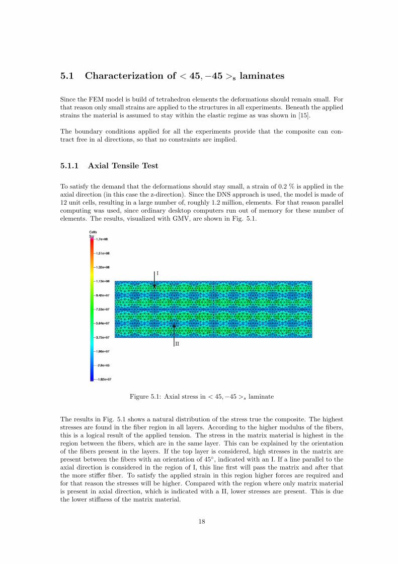
To satisfy the demand that the deformations should stay small, a strain of 0.2 % is applied in theaxial direction (in this case the z-direction). Since the DNS approach is used, the model is made of12 unit cells, resulting in a large number of, roughly 1.2 million, elements. For that reason parallelcomputing was used, since ordinary desktop computers run out of memory for these number ofelements. The results, visualized with GMV, are shown in Fig. 5.1.

Figure 5.1: Axial stress in < 45,−45 >s laminate

The results in Fig. 5.1 shows a natural distribution of the stress true the composite. The higheststresses are found in the fiber region in all layers. According to the higher modulus of the fibers,this is a logical result of the applied tension. The stress in the matrix material is highest in theregion between the fibers, which are in the same layer. This can be explained by the orientationof the fibers present in the layers. If the top layer is considered, high stresses in the matrix arepresent between the fibers with an orientation of 45◦, indicated with an I. If a line parallel to theaxial direction is considered in the region of I, this line first will pass the matrix and after thatthe more stiffer fiber. To satisfy the applied strain in this region higher forces are required andfor that reason the stresses will be higher. Compared with the region where only matrix materialis present in axial direction, which is indicated with a II, lower stresses are present. This is duethe lower stiffness of the matrix material.

18

5.1.2 Transverse Tensile Test

According to the axial tensile test, the applied strain and boundary conditions in this case are thesame, only applied in the transverse direction, namely the x-direction. Also in this case 12 unitcells are coupled to create the final structure. The results of the transverse tensile test are shownin Fig. 5.2.

Figure 5.2: Transverse stress in < 45,−45 >s laminate

As was observed in the case of the axial tensile test, also in this situation the highest stressesare found in the fibers, depicted with a III. The same holds for the stresses in the matrix region(indicated with a IV), where the stresses are the lowest. This is a logical consequence since theorientations of the fibers are only changed within the different layers, but the overall response ofthe composite does not change. The fibers with orientation of 45◦ are not situated in the topand bottom layers but in the middle layers. The opposite holds for the fibers with orientations of−45◦. Therefore the response is similar to the case of axial tension.

5.1.3 Shear test

The boundary conditions of the shear test are chosen differently compared with the boundaryconditions of the previous experiments. This model is also made of 12 unit cells, but is symmetricin the xz-plane. Therefore symmetric boundary conditions are applied in this plane. Further ashear strain of 0.15% is applied to the model. The result of this experiment is presented in Fig.5.3.

Again the stresses in the fiber are the highest in the composite. In this case the fibers are loadedmore in the direction of the fiber orientation. Consequently the stresses in the matrix region Vare lower compared with the case of axial and transverse tensile test. Furthermore the stresses inthe matrix region VI are the lowest in the composite. The same explanation can be given as inthe axial and transverse tensile test.

19

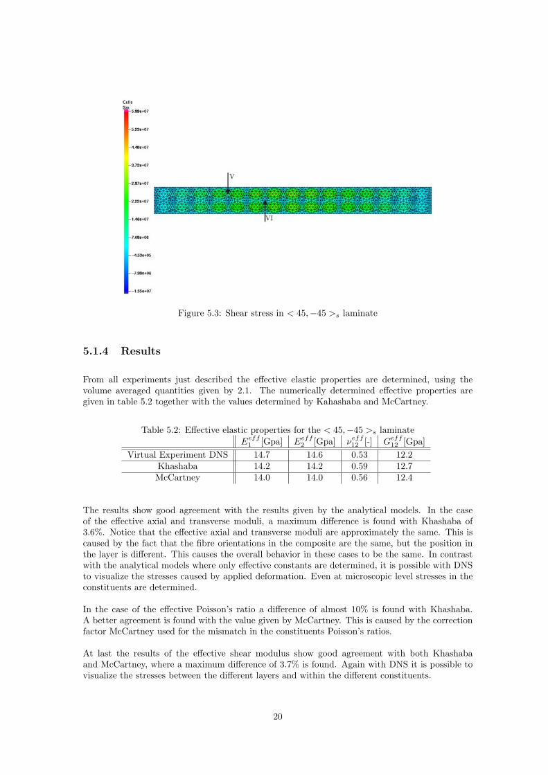
Figure 5.3: Shear stress in < 45,−45 >s laminate

5.1.4 Results

From all experiments just described the effective elastic properties are determined, using thevolume averaged quantities given by 2.1. The numerically determined effective properties aregiven in table 5.2 together with the values determined by Kahashaba and McCartney.

Table 5.2: Effective elastic properties for the < 45,−45 >s laminateEeff

1 [Gpa] Eeff2 [Gpa] νeff

12 [-] Geff12 [Gpa]

Virtual Experiment DNS 14.7 14.6 0.53 12.2Khashaba 14.2 14.2 0.59 12.7McCartney 14.0 14.0 0.56 12.4

The results show good agreement with the results given by the analytical models. In the caseof the effective axial and transverse moduli, a maximum difference is found with Khashaba of3.6%. Notice that the effective axial and transverse moduli are approximately the same. This iscaused by the fact that the fibre orientations in the composite are the same, but the position inthe layer is different. This causes the overall behavior in these cases to be the same. In contrastwith the analytical models where only effective constants are determined, it is possible with DNSto visualize the stresses caused by applied deformation. Even at microscopic level stresses in theconstituents are determined.

In the case of the effective Poisson’s ratio a difference of almost 10% is found with Khashaba.A better agreement is found with the value given by McCartney. This is caused by the correctionfactor McCartney used for the mismatch in the constituents Poisson’s ratios.

At last the results of the effective shear modulus show good agreement with both Khashabaand McCartney, where a maximum difference of 3.7% is found. Again with DNS it is possible tovisualize the stresses between the different layers and within the different constituents.

20

5.2 Characterization of < 0,±45,90 >s laminates

In this section the results of virtual experiments with < 0,±45, 90 >s laminates are presented.The FEM model for this laminate was already shown in Fig. 3.4, and is even more complex thanthe mesh for < 45,−45 >s laminates. This is mostly contributed to the multiple fiber orientationsin the composite. For all the experiments small strains are applied once more, since tetrahedronelements are used.

5.2.1 Axial Tensile Test

The applied strain of 0.2% is chosen, which is the same as in the case of < 45,−45 >s laminates.For this simulations 12 unit cells are coupled, which resulted in a lightly higher number of elementsof roughly 1.3 elements. That means that also for these experiments parallel computing is used.The results of the virtual experiment is presented in Fig. 5.4.

Figure 5.4: Axial stress in < 0,±45, 90 >s laminate

In this case the fibers with 0◦ orientation take most of the stress, because they are loaded intheir direction. Also the higher stiffness contributes to the higher stress concentration. Aroundthe fibers with 0◦ orientation, the stresses are low in the matrix region VII, caused by the lowerstiffness and no presence of fibers in the loading direction. For the stress concentration in thelayers containing the 45◦ and −45◦ the explanation can be given as discussed in section 5.1.1. Sothe high stresses in the matrix region are caused by the presence of fibres in the loading direction.

The highest stressed in the matrix are found in the region IX. This high stress concentrationis caused by the fibers with 90◦ orientation. Since there are fibers present in the loading directionin region IX, a higher force is required to deform the material. This causes the higher stress in thematrix region. For the region indicated with VIII, the stress is lower since in the loading directiononly matrix material is present, which has the smallest stiffness.

21

5.2.2 Transverse Tensile Test

In this case the same boundary conditions are applied to the composite as was shown in the caseof the axial tensile test, only applied in the transverse direction. Also this model contains 12 unitcells and the result of the transverse tensile test is shown in Fig. 5.5.

Figure 5.5: Transverse stress in < 0,±45, 90 >s laminate

The global response of the transverse tensile test is comparable with the response shown in theaxial tensile test. The difference with the axial tensile test is that the position of the fibers haschanged within the composite. The fibers oriented in the loading direction are no longer situatedin the layers on the boundary, but lie in the middle of the structure. Clearly visible is that themaximum stress is present in these fibers. The matrix region X around these fibers take less stress,since in the loading direction only matrix material is present. This could also be seen in the resultsof the axial tensile test.

Fibers oriented perpendicular to the loading direction contribute to a higher stress in the ma-trix region XI, where in the region XII the stresses are lower since in that region only matrixmaterial is present in the loading direction. This was also observed in the case of the axial tensiletest.

5.2.3 Shear test

At last the result for the shear test are shown. Compared with the experiment discussed in section5.1.3, the same boundary conditions are used for this experiment. So the boundary conditionsapplied, provide a symmetry condition. Also for this simulation 12 unit cells are coupled and theresult of the shear test is shown in Fig. 5.6.

The results show that the fibers with 45 and −45 take most of the stress. In comparison with theshear test discussed for the case of the < 45,−45 >s laminate this result is similar, since the fibers

22

Figure 5.6: Shear stress in < 0,±45, 90 >s laminate

are loaded nearly in the direction of their orientation. Consequently the matrix region XV takesless stress, which was also observed in the case of the < 45,−45 >s laminate.

Further presented in this figure is the high stress concentration in the top region XIII, wherethe 0◦ fibers are present. This is natural since the fibers have a higher modulus compared to thesurrounding matrix. In the layer containing the 90 oriented fibers, the stress distribution in thematrix is uniform. Since there is no constraint due to presence of fibers in the loading direction,the matrix deforms uniform in this region XIV.

5.2.4 Results

From the experiments described above, the effective elastic constant are determined using thevolume average quantities as given in equation (2.1). The results of the virtual experiments andthe results derived by McCartney are shown in table 5.3.

Table 5.3: Effective elastic properties for the < 0,±45, 90 >s laminateEeff

1 [Gpa] Eeff2 [Gpa] νeff

12 [-] Geff12 [Gpa]

Virtual Experiment DNS 153.8 153.7 0.26 57.6McCartney 151.9 151.9 0.27 59.8

For both the axial and transverse modulus good agreement is found with McCartney. The max-imum difference for both cases is 1.3%. Also in this case the axial and transverse modulus areroughly equal. This is due the fact that the global response is the same, caused by the same fibreorientations in the composite. The only difference is that the position of the oriented fibers ischanged in the total composite for the different loading cases.

A difference of 5.1% is found for the Poisson’s ratio with McCartney. However, McCartney madeassumptions in his model, so these experiments should describe the Poisson’s ratio more accurately.

23

For the shear modulus good agreement is found with McCartney, only a small difference of 3.6%is found. In contrast with the analytical values described by McCartney, with DNS it is possibleto predict the elastic properties and also visualize the stress concentrations in the total compositeon microscopic level.

24

Chapter 6

Conclusions andRecommendations

In this study an approach for mesh modeling of angle-ply laminated plates is presented. Thisapproach is based on (1) modeling the complex geometry of the fibers and matrix using booleanoperations and (2) using an automatic mesh generator (in this study provided by MSC Patran).This approach was used to create mesh models for < 45,−45 >s and < 0,±45, 90 >s laminatedcomposite plates, both with different volume fractions.

To verify the virtual experiments, the effective elastic constants were determined and comparedwith analytical values given in literature. The results of these virtual experiments showed goodagrement both with Khashaba and McCartney. In contrast with analytical models, with this DNSapproach it was possible to visualize the stresses on microscopic level in the different layers. Fromthese results it could be concluded that the influence of the fibre orientation was the mayor contri-bution in the matrix regions. Fibres orientated at an angle, different from the loading direction,caused higher stresses in the matrix region between these fibers. Also high stresses in the fibersorientated in the loading direction were visualized.

Compared with the analytical models, DNS gives a more accurate description of the elastic con-stants since no assumptions are made. Both Khashaba and McCartney assumed plane stress.Since DNS relies on direct modeling of the microstructure in 3D, naturally no assumptions likeplane-stress are made. Due to this modeling of the full microstructure the number of elementsincreased to 1.3 million. To execute the simulations parallel computing was necessary, and in thisresearch IPSAP was used as FEM program.

25

Recommendations

As presented in this study, the mesh of the complex geometries is based on tetrahedron elements.If larger deformation are involved these elements could cause problems, like overstiffening of thestructure or locking. In order to provide these consequences the mesh should be made out ofhexahedron elements. The automatic mesh generator of MSC PATRAN is not capable of meshingcomplex geometries with hexahedron elements, so a different mesh programm should be used.

As was shown the modeling of the fibers, the cross section was made of an octagonal shape.To describe the interface between the fiber and matrix and global behavior of the composite moreaccurately, a circular cross section should be used to create the geometry of the fibers.

Finally if the both hexahedron and circular cross section are implemented, delamination anddamage initiation could be analyzed under different loading geometries. Since TMCs are loadedunder extreme conditions, this should be investigated in further research.

26

References

[1] J. Kuk Hyun. Direct Numerical Simulation on Micromechanical Behaviors of CompositeMaterials and Strucures. PhD thesis, Seoul National University, 2006.

[2] ASTM. Standards and literature referendes for composite materials. 2nd ed., West Con-shohocken, PA: ASTM, 1990.

[3] S.G. Warrier and R. Y. Lin. Infrared infiltration and properties of scs-6/ti alloy composites.Journal of Materials Science, 31:1821–1828, 1996.

[4] B.A. Bednarcyk and S.M. Arnold. New local failure model with application to the longtitu-dinal tensile behaviour of continuously reinforced titanium composites with local debonding.Composites Science and Technology, 61:705–729, 2001.

[5] R.R. Boyer and H.W. Rosenberg, editors. Ti-15-3 Property Data. Proceedings of Beta Tita-nium Alloys in the 80’s, 1983. Metallurgical Society, Atlanta.

[6] M.P. Thomas and M.R. Winstone. Effect of matrix alloy on longitudinal tensile behaviour offibre reinforced titanium matrix composites. Scripta Materiallia, 37:1855–1862, 1997.

[7] L.N. McCartney and A. Kelly. Effective thermal and elastic properties of < +θ,−θ > lami-nates. Composites Science and Technology, Article in Press, 2006.

[8] T.W. Clyne. A compressibility-based derivation of simple expressions for the transversepoisson’s ratio and shear modulus of an aligned long fibre composite. Journal of MaterialsScience, 9:366–339, 1990.

[9] C.M.Chen and T.Y. Kam. Elastic constants identification of symmetric angle-ply laminatesvia a two-level optimization approach. Composites Science and Technology, Article in Press,2006.

[10] Z. Gurdal. Design and Optimization of Laminated Composite Materials. John Wiley & Sons,New York, 1999.

[11] C.T. Sun and R.S. Vaidya. Prediction of composite properties from a representative volumeelement. Composites Science and Technology, 56:171–179, 1996.

[12] J.H. Kim M Joh S.J. Kim, C.S. Lee and S. Lee. Ipsap: A high-performance parallel finiteelement code for large-scale structural analysis based on domain-wise multifrontal technique.SC’03,Phoenix, Arizona, USA, November 2003.

[13] H.J. Yeo J.H. Kim S.J. Kim, C.S. Lee and J.Y. Cho. Direct numerical simulation of compositestructures. Journal of Composite Materials, 36:2765–2784, 2002.

[14] Internet parallel structure analysis program (ipsap) user’s guide.http://aeroguy.snu.ac.kr/IPSAP/WEB/, February 2006.

27

[15] S.M. Arnold B.A. Bednaryck and B.A. Lerch. Damage and failure prediction for sic/ti-15-3laminates. NASA/TM-2001-211343, December 2001.

[16] T.J.R. Hughes. The finite element method, linear static and dynamic finiti element analysis.Prentice-Hall, Inc., Englewood Cliffs, NJ, 1987.

[17] U.A. Khashaba. In-plane shear properties of cross-ply composite laminates with differentoff-axis angles. Composite Structures, 65:167–177, 2004.

[18] Functional Assignments. MSC PATRAN, 2005.

28

Appendix A

Derivation Stress Strain Relationfor Angle Lamina

The stress-strain relation for an orthotropic unidirectional lamina is given as

σx

σy

τxy

=

Q11 Q12 0Q12 Q22 00 0 Q66

εx

εy

γxy

, (A.1)

where Qij are the reduced stiffness coefficients, which are related to the elastic properties of thelaminate as

Q11 =E1

1− ν12ν21, Q22 =

E2

1− ν12ν21, Q12 =

ν12E2

1− ν12ν21and Q66 = G12. (A.2)

With this relation one can describe the stress-strain relation for an angle lamina.To describe the stress-strain relation for an angle lamina, the stresses and strains should betransformed to their new state. Consider picture (A.1).

The global (x-y) and local (1-2) stresses are related to the angle of the lamina, θ

σx

σy

τxy

= T−1

σ1

σ2

τ12

, (A.3)

where T is called the transformation matrix and is defined as

T =

c2 s2 2css2 c2 −2cs−cs cs c2 − s2

(A.4)

29

Figure A.1: Angle lamina

with c = cos(θ) and s = sin(θ). The relation between the global stress and local strain can bewritten as

σx

σy

τxy

= T−1Q

ε1

ε2

γ12

. (A.5)

To describe the global stress-strain relation, first the relation between the global and local strainsis described.

ε1

ε2

γ12/2

= T

εx

εy

γxy/2

(A.6)

Equation (A.6) can be written as

ε1

ε2

γ12/2

= RTR−1

εx

εy

γxy/2

(A.7)

where R is the Reuter matrix and is defined as

R =

1 0 00 1 00 0 2

. (A.8)

Substituting equation (A.7) in equation (A.5) gives

σx

σy

τxy

= T−1QRTR−1

εx

εy

γxy

. (A.9)

30

Working out the multiplication of the five matrices in equation (A.9) gives

σx

σy

τxy

=

Q11 Q12 Q16

Q12 Q22 Q26

Q16 Q26 Q66

εx

εy

γxy

, (A.10)

where Qij are called the elements of the transformed reduced stiffness matrix Q, where

Q11 = Q11c4 + Q22s

4 + 2(Q12 + 2Q66)s2c2,

Q12 = (Q11 + Q22 − 4Q66)s2c2 + Q12(c4 + s2),Q22 = Q11s

4 + Q22c4 + 2(Q12 + 2Q66)s2c2,

Q16 = (Q11 −Q12 − 2Q66)c3s− (Q22 −Q12 − 2Q66)s3c,

Q26 = (Q11 −Q12 − 2Q66)cs3 − (Q22 −Q12 − 2Q66)c32,

Q66 = (Q11 + Q22 − 2Q12 − 2Q66)s2c2 + Q66(s4 + c4). (A.11)

31

Appendix B

Correction factors

As presented in section 4.2.2 McCartney used correction factors for determining the elastic prop-erties of angle-ply laminates. The correction factor λ1, which is used for calculations of E1 andν12, is given by

1λ1

=12

[1

Gm+

Vf

Km+

Vm

Kf

]. (B.1)

In equation (B.1) Gm is the shear modulus and Km the bulk modulus of the matrix material,where Kf is the bulk modulus of the fibre material.

The correction factor λ2 is used to describe the shear modulus G12, where λ2 is:

1λ2

= Gm(1 + Vf ) + GfVm. (B.2)

To determine the transverse modulus E2 of a single lamina McCartney used the transverse bulkmodulus Kt and the transverse shear modulus Gt, according to,

1Kt

=Vf

Kf+

Vm

Km− λ1

2

(1

Kf− 1

Km

)2

VfVm, (B.3)

Gt = VfGf + VmGm − λ3(Gf −Gm)2VfVm, (B.4)

where,

1λ3

= VmGf + VfGm +KmGm

Km + 2Gm. (B.5)

33