journal of american science, 2012;8(3) ... · journal of american science, 2012;8 ... a main...
TRANSCRIPT
Journal of American Science, 2012;8(3) http://www.americanscience.org
http://www.americanscience.org [email protected] 565
Mathematical Modeling of Tall Buildings and its Foundation under Randomly Fluctuating Wind and Earthquake Ground Motions
Aly El-Kafrawy
Production Engineering and Mechanical Design Dept., Faculty of Engineering,
Port-Said University, Port-Said, Egypt [email protected]
Abstract: In the present paper, a non-dimensional mathematical model for high tower buildings and its foundation under randomly fluctuating wind loads and earthquake ground motions excitations is developed as a nonlinear model to study the system more extensively. The system main equations could be derived using two different derivation methods and linearized in minimal symbolic forms; which facilitate a subsequent numerical simulation in order to investigate the vibration characteristics of whole system. The analysis enables designers to have more insight into the characteristics of high tower buildings of similar configuration but with different geometry and material. The complexity of wind loading with its variations in space and time has been considered. A comprehensive mathematical model of six degrees of freedom is presented and solved for free and forced vibrations. [Aly El-Kafrawy. Mathematical Modeling of Tall Buildings and its Foundation under Randomly Fluctuating Wind and Earthquake Ground Motions. Journal of American Science 2012; 8(3):565-588]. (ISSN: 1545-1003). http://www.americanscience.org. 76 Keywords tall building vibrations, modal analysis, foundation vibrations, power spectral density, random wind excitation, earthquake ground motions Introduction and literature review Large investments have recently been made for the construction of new medium- and high-rise buildings in the world. In many cases performance-based designs have been the preferred method for these buildings. A main consideration in performance-based seismic design is the estimation of the likely development of structural and nonstructural damage limit-states given a hazard level. For this type of buildings efficient modeling techniques are required able to compute the response at different performance states. Certain structures are less vulnerable against vibration impacts whereas certain others are more vulnerable. As we all know that vibration effects are now cannot be neglected, as our day to day life is affected by them. Study of vibration responses of structures has always been a principal concern for design engineers. Therefore, we do put an eye on the vibrations of buildings and its foundations. Uncontrolled vibration causes devastation. Occurrences of Tsunami, earthquake, collapse of structures are few such most common devastating effects of vibration. Thus the study of vibration responses in advance is of immense importance for sustainable and positive effects of vibrations for the well being of humans. Nowadays, the new and emerging concept of seismic structural design, the so-called performance-based design, requires careful consideration of all aspects involved in structural analysis. One of the most important aspects of structural analysis is Soil-Structure Interaction (SSI). Such interaction may alter
the dynamic characteristics of structures and consequently may be beneficial or detrimental to the performance of structures. Soil conditions at a given site may amplify the response of a structure on a soil deposit. Not taking into account these structural response amplifications may lead to an under-designed structure resulting in a premature collapse during an earthquake. Analytical methods of SSI concentrate mainly on single degree of freedom systems and analysis/design of long and important structures such as large bridges and nuclear power plants, and rarely on regular type buildings. Studies which include SSI effects will help to better predict the performance of structures during future ground motions. State of the art knowledge and analytical approaches require, that, the structure-foundation system to be represented by mathematical models that include the influence of the sub-foundation media. A research work of Panagiotou (2008) was conducted at University of California San Diego (UCSD) on the seismic design, experimental response, and computational modeling of medium- and high-rise reinforced concrete wall buildings. Kim (2008) presented an investigation of the effect of vertical ground motion on reinforced concrete structures studied through a combined analytical-experimental research approach. Krier (2009) analyzed several soil-structure interaction problems. Buildings on elastic foundations were studied and comparisons were made between analytical results and the solutions obtained from a Tera Dysac finite element analysis. Gouasmia et al. (2009) studied the

Journal of American Science, 2012;8(3) http://www.americanscience.org
http://www.americanscience.org [email protected] 566
seismic response of an idealized small city composed of five equally spaced, five storey reinforced concrete buildings anchored in a soft soil layer overlaid by a rock half space. These results show response amplification of the buildings in the near field in accordance with the results observed in similar cases. Antonyuk, Timokhin (2007) outlined a mathematical model describing the vibrations of buildings and engineering structures with general-type passive shock-absorbers, rigid bodies, and ideal constraints. Auersch (2008) predicted a practice-oriented environmental building vibrations. A Green’s functions method for layered soils is used to build the dynamic stiffness matrix of the soil area that is covered by the foundation. A simple building model is proposed by adding a building mass to the dynamic stiffness of the soil. Belakroum et al. (2008) studied the numerical prediction of the aerodynamic behaviour of rectangular buildings. Simulations were made for rectangles of different side coefficients and different angles of attack. The finite element method is used to simulate fluid flow considered Newtonian and incompressible. Davoodi, et al. (2008) used the ambient vibration tests to rely on natural excitations, consequently, it was recommended to perform impulsive test for identifying the hidden dynamic characteristics of the building. Kuźniar and Waszczyszyn (2006) applied neural networks for computation of fundamental natural periods of buildings with load-bearing walls. The analysis is based on long-term tests performed on actual buildings. The identification problem was formulated as the relation between structural and soil basement parameters, and the fundamental period of building. Uzdin, et al. (2009) derived equations for the vibrations of a building on the foundations under consideration. Impossibility of use of traditional methods of the linear-spectral theory for analysis of their earthquake resistance is demonstrated. It is established that the systems under consideration do not possess a natural vibration period, and may have ambiguous solutions for forced vibrations. The influence of city traffic-induced vibration on Vilnius Arch-Cathedral Belfry was investigated (Kliukas et al. 2008). Two sources of dynamic excitation were studied. Conventional city traffic was considered to be a natural source of excitation while excitation imposed artificially by moving a heavily loaded truck was considered to be the source of increased risk excitation. Configuration of equipment on springs is simplified for numerical analysis. A simplified approach and associated equations of motion can be developed to evaluate the response of the equipment with vertical and horizontal forcing functions (Turner 2004). Gong (2010) developed a free
vibration analysis method for space mega frames of super tall buildings. The physical model of a mega frame was idealized as a three-dimensional assemblage of stiffened close-thin-walled tubes with continuously distributed mass and stiffness. Yang et al. (2008) analyzed the wave propagation problems caused by the underground moving trains by the 2.5-dimensional finite/infinite element approach. The near field of the half-space, including the tunnel and parts of the soil, was simulated by finite elements, and the far field extending to infinity by infinite elements. Ground-borne vibrations due to subway trains have sometimes reached the level that cannot be tolerated by residents living in adjacent buildings (Shyu et. al. 2002). Also, approaches for predicting vibrations caused by metro trains moving through the tunnel were developed (Gupta et al. 2007), e.g., a semi-analytical pipe-in-pipe model (Forrest and Hunt 2006a,b) and a coupled periodic finite-element–boundary-element model (Clouteau et al. 2005; Degrande et al. 2006b). Clearly, ground-borne vibrations have become an issue of great concern, which will continuously attract the attention of researchers and engineers worldwide. Many research projects on ground-borne vibrations due to subway trains were conducted by field measurement (Vadillo et al. 1996; Degrande et al. 2006a) and empirical or semiempirical prediction models (Kurzweil 1979; Trochides 1991; Melke 1998). These studies provide practical references for solving related problems. However, most of these studies were performed for a specific condition, thereby suffering from the lack of generality. On the other hand, concerning the techniques of simulation, most previous works have been based on the two-dimensional (2D) models (Balendra et al. 1991; Yun et al. 2000; Metrikine and Vrouwenvelder 2000). Prowell (2011) presented an experimental and numerical investigation into the seismic response of modern wind turbines simultaneously subjected to wind, earthquake, and operational excitation. Ulusoy (2011) described a certain class of system identification algorithms with particular emphasis on civil engineering applications. The algorithms originated from system realization theory enabled one to identify finite dimensional, linear, time-invariant models of systems in the state space representation from observed data. Wieser (2011) used OpenSees finite element framework to develop full three dimensional models of four steel moment frame buildings. The incremental dynamic analysis method is employed to evaluate the floor response of inelastic steel moment frame buildings subjected to all three components of a suite of 21 ground motions. Ghafari Oskoei (2011) dealt with the dynamic behavior of tall guyed masts under seismic loads. Zhong (2011)
Journal of American Science, 2012;8(3) http://www.americanscience.org
http://www.americanscience.org [email protected] 567
utilized a ground motion acceleration time-history as an input to an analytic model of a structure and solved the structural response at each time step of the ground motion record. Weng (2010) proposed a forward substructuring approach, the eigenproperties of the partitioned substructures were assembled to recover the eigensolutions and eigensensitivities of the global structure, which were tuned to reproduce the experimental measurements through an optimization process. Sonmez (2010) developed semi- active controllers, which were based on real-time estimation of instantaneous (dominant) frequency and the evolutionary power spectral density by time-frequency analysis of either the excitation or the response of the structure. Time-frequency analyses were performed by either short-time Fourier transform or wavelet transform. Soudkhah (2010) examined the dynamic response of surface foundations on sandy soils under both forced and ground motion disturbance. Yao (2010) used the direct method for modeling the soil and a tall building together and studied energy transferring from soils to buildings during earthquakes, which is critical for the design of earthquake resistant structures and for upgrading existing structures. Ahearn (2010) studied the dynamic effects of wind-induced vibrations on high-mast structures and proposed several retrofits that increase the aerodynamic damping, thereby reducing vibrations. The ground vibration induced by earthquake ground motions is a complicated dynamic problem due to the involvement of a number of factors along the paths of wave propagation, including the load generation mechanism, the geometry and location of tunnel structures, the irregularity of soil layers, etc. Previously, many research projects on ground-borne vibrations due to earthquakes were conducted by field measurement and empirical or semi-empirical prediction models. These studies provide practical reference for solving related problems. However, most of these studies were performed for a specific condition, thereby suffering from the lack of generality. Assumptions 1. The high tower building-foundation equivalent
system moves only in the y*- z* plane. 2. The wind effect is identified as randomly
fluctuating wind loads in horizontal direction. 3. Uy(t), UZ(t) are random ground motions of
earthquake in horizontal and vertical directions y and z.
4. The high tower building and its foundation are assumed as rigid bodies.
5. The soil kind under the foundation is assumed as a sandy clay.
6. The angular velocities ),t( ),t( *1
*o and )t(*
2 are
very small (<<1). 7. The equivalent spring stiffness k k EHH ,, and
vk are linear.
8. The equivalent damping coefficients r r EHH ,, and
vr are linear.
9. The density of building 2 is taken as 0.1 that of
the foundation. 10.The air friction was not considered.
11.The place pressure factor pC can be replaced
through the average load factor of total building.
12.The spectral power density )(S11UU is
independent on the Cartesian Coordinates z, y. 13.The wind velocity distribution along the height of
the building is )H(U)H
z()z(U .
14.The cross spectral power density )(S21UU can
be represented through the coherence spectrum of
the wind velocity )t,z(U 1' and )t,z(U 2
' :
)](S . )(S[)(S)(22112121 UUUU
2
UU2
UU
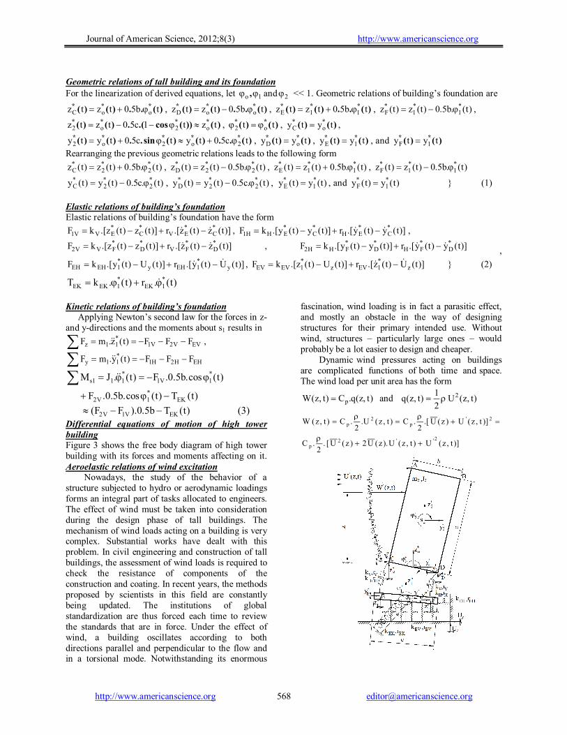
Derivation of system equations using D’alembert’s principle The model of the problem to be considered is schematically shown in Fig. 1. This model describing the vibrations of high-tower building and its foundation with general-type equivalent passive springs and dampers, rigid bodies, and some ideal constraints like linear springs and dampers under the effect of randomly fluctuating wind loads and the excitation of earthquake ground motions. In setting up the equations of motion of the equivalent system in Fig. 1, it should be born in mind that the geometric, elastic, and kinetic relations of both high tower building and its foundation must be derived. Moreover the external excitation of wind loads should be prepared. Foundation differential equations of motion Figure 2 shows the free body diagram of foundation with its accompanied vibrating soil.
Journal of American Science, 2012;8(3) http://www.americanscience.org
http://www.americanscience.org [email protected] 568
Geometric relations of tall building and its foundation For the linearization of derived equations, let and 21o , << 1. Geometric relations of building’s foundation are
)(..)()( *** tb50tztz ooC , )(..)()( *** tb50tztz ooD , )(..)()( *** tb50tztz 11E , )t(.b5.0)t(z)t(z *1
*1
*F ,
)())(cos.(.)()( **** tzt1c50tztz o2o2 , )()( ** tt o2 , )()( ** tyty oC ,
)(..)()(sin..)()( ***** tc50tytc50tyty 2o2o2 , )()( ** tyty oD , )()( ** tyty 1E , and )()( ** tyty 1F
Rearranging the previous geometric relations leads to the following form
)t(.b5.0)t(z)t(z *2
*2
*C , )t(.b5.0)t(z)t(z *
2*2
*D , )t(.b5.0)t(z)t(z *
1*1
*E , )t(.b5.0)t(z)t(z *
1*1
*F
)t(.c5.0)t(y)t(y *2
*2
*C , )t(.c5.0)t(y)t(y *
2*2
*D , )t(y)t(y *
1*E , and )t(y)t(y *
1*F } (1)
Elastic relations of building’s foundation Elastic relations of building’s foundation have the form
)]t(z)t(z.[r)]t(z)t(z.[kF *C
*EV
*C
*EVV1 , )]t(y)t(y.[r)]t(y)t(y.[kF *
C*EH
*C
*EHH1 ,
)]t(z)t(z.[r)]t(z)t(z.[kF *D
*FV
*D
*FVV2 , )]t(y)t(y.[r)]t(y)t(y.[kF *
D*FH
*D
*FHH2
,
)]t(U)t(y.[r)]t(U)t(y.[kF y*1EHy
*1EHEH
, )]t(U)t(z.[r)]t(U)t(z.[kF z*1EVz
*1EVEV
} (2)
)t(.r)t(.kT *1EK
*1EKEK
Kinetic relations of building’s foundation Applying Newton’s second law for the forces in z- and y-directions and the moments about s1 results in
EVV2V1*11z FFF)t(z.mF ,
EHH2H1*11y FFF)t(y.mF
)t(cos.b5.0.F)t(.JM *1V1
*111s
)t(T)t(cos.b5.0.F EK*1V2
(3) )t(Tb5.0).FF( EKV1V2
Differential equations of motion of high tower building Figure 3 shows the free body diagram of high tower building with its forces and moments affecting on it. Aeroelastic relations of wind excitation
Nowadays, the study of the behavior of a structure subjected to hydro or aerodynamic loadings forms an integral part of tasks allocated to engineers. The effect of wind must be taken into consideration during the design phase of tall buildings. The mechanism of wind loads acting on a building is very complex. Substantial works have dealt with this problem. In civil engineering and construction of tall buildings, the assessment of wind loads is required to check the resistance of components of the construction and coating. In recent years, the methods proposed by scientists in this field are constantly being updated. The institutions of global standardization are thus forced each time to review the standards that are in force. Under the effect of wind, a building oscillates according to both directions parallel and perpendicular to the flow and in a torsional mode. Notwithstanding its enormous
fascination, wind loading is in fact a parasitic effect, and mostly an obstacle in the way of designing structures for their primary intended use. Without wind, structures – particularly large ones – would probably be a lot easier to design and cheaper.
Dynamic wind pressures acting on buildings are complicated functions of both time and space. The wind load per unit area has the form
)t,z(q.C)t,z(W p and )t,z( U2
1)t,z(q 2
)]t,z(U)t,z(U).z(U2)z(U[ .2
.C
)]t,z(U)z(U.[2
.C)t,z(U.2
.C)t,z(W
2''2p
2'p
2p

Journal of American Science, 2012;8(3) http://www.americanscience.org
http://www.americanscience.org [email protected] 569
Fig. 1 Equivalent system of tall building and its foundation
Fig. 2 Free body diagram of foundation with its
accompanied vibrated soil
),()(),().(.)(..),( '' tzW zWtzUzU.C zU 2
CtzW p2
p
The total turbulent wind force in y*-direction as a function of time is
c
0
c
0p dz tzUzU.C dz tzWtW ),().(.),()( '' (4)
The total turbulent wind moment as a function of time is
c
0
'*2
*2W dz )t,z(W))].t(sin
2
b)t(cos
2
c(z[)t(M
c
0
' dz )t,z(W).2
cz(
c
0
'p dz )t,z(U).z(U..C ).
2
cz( (5)
Fig. 3 Free body diagram of the high tower building Elastic relations of high tower building
Elastic relations of high tower building have the form
)]t(z)t(z.[r)]t(z)t(z.[kF *E
*CV
*E
*CVV1 , )]t(y)t(y.[r)]t(y)t(y.[kF *
E*CH
*E
*CHH1
)]t(z)t(z.[r)]t(z)t(z.[kF *F
*DV
*F
*DVV2 , )]t(y)t(y.[r)]t(y)t(y.[kF *
F*DH
*F
*DHH2 (6)
Kinetic relations of high tower building Applying Newton’s second law for the forces in z and y-directions and also the moments about s2 results in
V2V1*22z FF)t(z.mF , )t(WFF)t(y.mF H2H1
*22y
)](cos.)(sin..[)(. *** t2
bt
2
cFtJM 22V1222s )](sin.
2)(cos.
2.[ *
2*21 t
bt
cF H
)]t(cos.2
b)t(sin.
2
c.[F *
2*2V2 )t(M)]t(sin.
2
b)t(cos.
2
c.[F W
*2
*2H2 } (7)
The previous equation can be linearized in the following form
]2
c)t(.
2
b.[F)]t(.
2
c
2
b.[FM *
2H1*2V12s )t(M]
2
c)t(.
2
b.[F)]t(.
2
c
2
b.[F W
*2H2
*2V2
Deriving the system’s differential equations of motion

Journal of American Science, 2012;8(3) http://www.americanscience.org
http://www.americanscience.org [email protected] 570
Application of the geometric relations of the foundation Substitute from Eqs. 1 in Eqs. 2 of the elastic relations of foundation free body diagram
)](.5.0)()(.5.0)(.[)](.5.0)()(.5.0)(.[ *2
*2
*1
*1
*2
*2
*1
*11 tbtztbtzrtbtztbtzkF VVV
)]t(c5.0)t(y)t(y.[r)]t(c5.0)t(y)t(y.[kF *2
*2
*1H
*2
*2
*1HH1
)](.5.0)()(.5.0)(.[)](.5.0)()(.5.0)(.[ *2
*2
*1
*1
*2
*2
*1
*12 tbtztbtzrtbtztbtzkF VVV } (8)
)](5.0)()(.[)](5.0)()(.[ *2
*2
*1
*2
*2
*12 tctytyrtctytykF HHH
Application of the elastic relations of the foundation
Substitute from Eqs. 2 of foundation’s elastic relations in Eqs. 3 of its kinetic relations results in
)()(.)(.2)().2()(2)().2()(. *2
*1
*2
*1
*11 tUrtUktzrtzrrtzktzkktzm zEVzEVVVEVVVEV
)().2()(.)(.2)().2()(. *1
*2
*2
*1
*11 tyrrtcktyktykktym HEHHHHEH
} (9)
)(.)(.)(.)(.2 *2
*2 tUrtUktcrtyr yEHyEHHH
)(..5.0)(]..5.0[)(..5.0)(]..5.0[)(. *2
2*1
2*2
2*1
2*11 trbtrbrtkbtkbktJ VVEKVVEK
Application of the geometric relations of the building Substitute from Eqs. 1 of geometric relations in Eqs. 6 of elastic relations of the building
)](.5.0)()(.5.0)(.[)](.5.0)()(.5.0)(.[ *1
*1
*2
*2
*1
*1
*2
*21 tbtztbtzrtbtztbtzkF VVV
)](5.0)()(.[)](5.0)()(.[ *2
*2
*1
*2
*2
*11 tctytyrtctytykF HHH } (10)
)](.5.0)()(.5.0)(.[)](.5.0)()(.5.0)(.[ *1
*1
*2
*2
*1
*1
*2
*22 tbtztbtzrtbtztbtzkF VVV
)]t(c5.0)t(y)t(y.[r)]t(c5.0)t(y)t(y.[kF *2
*2
*1H
*2
*2
*1HH2
Application of the elastic relations of the building Substitute Eqs. 10 of building’s elastic relations in Eqs. 7 of its kinetic relations lead to the following differential equations
)(.)(.)(.)(.)(. ***** tzr2tzr2tzk2tzk2tzm 2V1V2V1V22
)()](.)(.2)(.2)(.)(.2)(.2)(. *2
*2
*1
*2
*2
*1
*22 tWtcrtyrtyrtcktyktyktym HHHHHH } (11)
)()..5.0.5.0()(.)(..5.0)(.)(. *2
22*2
*1
2*1
*22 tkbkctycktkbtycktJ VHHVH
)t(M)t().r.b5.0r.c5.0()t(y.cr)t(.r.b5.0)t(y.cr W*2V
2H
2*2H
*1V
2*1H
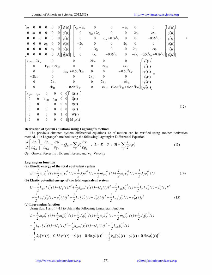
Arranging the differential equations of motion The differential equations of motion of both tall building and its foundation can be summarized in the form
)()(.)(2)().2()(.2)().2()(. *2
*1
*2
*1
*11 tUrtUktzktzkktzrtzrrtzm zEVzEVVVEVVVEV
)(.)(.2)().2()(.)(.2)().2()(. *2
*2
*1
*2
*2
*1
*11 tcktyktykktcrtyrtyrrtym HHHEHHHHEH
)t(U.r)t(Uk yEHyEH
0)(..5.0)()..5.0()(..5.0)(]..5.0[)(. *2
2*1
2*2
2*1
2*11 tkbtkbktrbtrbrtJ VVEKVVEK
0tzk2tzk2tzr2tzr2tzm 2V1V2V1V22 )(.)(.)(.)(.)(. *****
)()(.)(.2)(.2)(.)(.2)(.2)(. *2
*2
*1
*2
*2
*1
*22 tWtcktyktyktcrtyrtyrtym HHHHHH
)()..5.0.5.0()(.)(..5.0)(.)(. *2
22*2
*1
2*1
*22 trbrctycrtrbtycrtJ VHHVH
)()()..5.0.5.0()(.)(..5.0)(. *2
22*2
*1
2*1 tMtkbkctycktkbtyck WVHHVH
Journal of American Science, 2012;8(3) http://www.americanscience.org
http://www.americanscience.org [email protected] 571
)(
)(
)(
)(
)(
)(
)5.05.0(05.00
20020
002002
5.0005.000
20020
002002
)(
)(
)(
)(
)(
)(
00000
00000
00000
00000
00000
00000
*2
*2
*2
*1
*1
*1
222
22
*2
*2
*2
*1
*1
*1
2
2
2
1
1
1
t
ty
tz
t
ty
tz
rbrccrrbcr
crrr
rr
rbrbr
crrrr
rrr
t
ty
tz
t
ty
tz
J
m
m
J
m
m
VHHVH
HHH
VV
VVEK
HHHEH
VVEV
+
)(
)(
)(
)(
)(
)(
)..(.
..
*
*
*
*
*
*
t
ty
tz
t
ty
tz
kb50kc50ck0kb50ck0
ckk200k20
00k200k2
kb5000kb50k00
ckk200k2k0
00k200k2k
2
2
2
1
1
1
V2
H2
HV2
H
HHH
VV
V2
V2
EK
HHHEH
VVEV
)(
)(
)(
)(
)(
)(
tM
tW
t
t
t
t
100000
010000
000000
000000
00rk00
0000rk
W
EHEH
EVEV
(12)
Derivation of system equations using Lagrange’s method
The previous obtained system differential equations 12 of motion can be verified using another derivation method, like Lagrange’s method using the following Lagrangian Differential Equation
i K
iiK
KKK qFQ
L
q
L
dt
d
, L = E – U ,
n
2nnr
2
1 (13)
QK : General forces, Fi : External forces, and i : Velocity
Lagrangian function (a) Kinetic energy of the total equivalent system
)t(J2
1)t(ym
2
1)t(zm
2
1)t(J
2
1)t(ym
2
1)t(zm
2
1E
222222 *22
*22
*22
*11
*11
*11 (14)
(b) Elastic potential energy of the total equivalent system
2*C
*EV
*1EK
2y
*1EH
2z
*1EV )]t(z)t(z[k
2
1)t(k
2
1)]t(U)t(y[k
2
1)]t(U)t(z[k
2
1U
2
2*D
*FH
2*D
*FV
2*C
*EH )]t(y)t(y[k
2
1)]t(z)t(z[k
2
1)]t(y)t(y[k
2
1 (15)
(c) Lagrangian function Using Eqs. 1 and 14-15 to obtain the following Lagrangian function
)t(J2
1)t(ym
2
1)t(zm
2
1)t(J
2
1)t(ym
2
1)t(zm
2
1L
222222 *22
*22
*22
*11
*11
*11
)t(k2
1)]t(U)t(y[k
2
1)]t(U)t(z[k
2
1 2*1EK
2y
*1EH
2z
*1EV
2*2
*2
*1
2*2
*2
*1
*1 )](.5.0)()([
2
1)](.5.0)()(.5.0)([
2
1tctytyktbtztbtzk HV

Journal of American Science, 2012;8(3) http://www.americanscience.org
http://www.americanscience.org [email protected] 572
2*2
*2
*1
2*2
*2
*1
*1 )](.5.0)()([
2
1)](.5.0)()(.5.0)([
2
1tctytyktbtztbtzk HV (16)
Rayleigh’s dissipation function
The Rayleigh’s dissipation function can be derived as
)t(r2
1)]t(U)t(y[r
2
1)]t(U)t(z[r
2
1r
2
1 2*1EK
2y
*1EH
2z
*1EV
61n
266
2*2
*2
*1H
2*2
*2
*1
*1V )]t(.c5.0)t(y)t(y[r
2
1)]t(.b5.0)t(z)t(.b5.0)t(z[r
2
1
2*2
*2
*1
2*2
*2
*1
*1 )](.5.0)()([
2
1)](.5.0)()(.5.0)([
2
1tctytyrtbtztbtzr HV (17)
General external forces
i K
ii
i K
iiK
q
rF
qFQ
, Where **
2221W21 and , y , MF , WF
Deriving the differential equations of motion
(a) Case of )(* tzq 11
)(.)(
**
tzmtz
L
dt
d11
1
, )(.)(.2)()2(
)(*2
*1*
1
tUktzktzkktz
LzEVVVEV
)(.)(.)().()(
***
tUrtzr2tzr2rtz
zEV2V1VEV1
, and 0Q *
1z
Substitute from the equations of case (a) in Eq. 13, the first differential equation of motion can be obtained
)()(.)(2)().2()(.2)().2()(. *2
*1
*2
*1
*11 tUrtUktzktzkktzrtzrrtzm zEVzEVVVEVVVEV
(18)
(b) Case of )(* tyq 12
)t(y.m)t(y
L
dt
d *11*
1
, )t(Uk)t(.ck)t(y.k2)t(y).kk2(
)t(y
LyEH
*2H
*2H
*1EHH*
1
)t(Ur)t(.cr)t(y.r2)t(y).rr2()t(y
yEH*2H
*2H
*1EHH*
1
, and 0Q *
1y
Substitute from the equations of case (b) in Eq. 13, the second differential equation of motion can be obtained
)(.)(.2)().2()(.)(.2)().2()(. *2
*2
*1
*2
*2
*1
*11 tcktyktykktcrtyrtyrrtym HHHEHHHHEH
)t(U.r)t(Uk yEHyEH (19)
(c) Case of )(* tq 13
)t(.J)t(
L
dt
d *11*
1
, )t(.k
2
b)t().k
2
bk(
)t(
L *2V
2*1V
2
EK*1
)t(.r2
b)t().r
2
br(
)t(
*2V
2*1V
2
EK*1
, and 0Q *
1
Substitute from the equations of case (c) in Eq. 13, the third differential equation of motion can be obtained
0)(..5.0)()..5.0()(..5.0)(]..5.0[)(. *2
2*1
2*2
2*1
2*11 tkbtkbktrbtrbrtJ VVEKVVEK (20)
(d) Case of )t(zq *24
)t(z.m)t(z
L
dt
d *22*
2
, )t(z.k2)t(z.k2
)t(z
L *2V
*1V*
2

Journal of American Science, 2012;8(3) http://www.americanscience.org
http://www.americanscience.org [email protected] 573
)t(z.r2)t(z.r2z
*2V
*1V*
2
, and 0Q *
2z
Similarly, the fourth differential equation of motion can be obtained
0)(.2)(.2)(.2)(.2)(. *2
*1
*2
*1
*22 tzktzktzrtzrtzm VVVV
(21)
(e) Case of )t(yq *25
)t(y.m)t(y
L
dt
d *22*
2
, )t(.ck)t(y.k2)t(y.k2
)t(y
L *2H
*2H
*1H*
2
)t(.cr)t(y.r2)t(y.r2)t(y
*2H
*2H
*1H*
2
, and )t(WQ *
2y
Similarly, the fifth differential equation of motion can be obtained
)(.)(.2)(.2.)(.2)(.2)(. *2
*2
*1
*2
*2
*1
*22 tWcktyktykcrtyrtyrtym HHHHHH (22)
(f) Case of *26q
)t(.J)t(
L
dt
d *22*
2
, )t().k
2
bk
2
c()t(y.ck)t(.k
2
b)t(y.ck
)t(
L *2V
2
H
2*2H
*1V
2*1H*
2
)t().r2
cr
2
b()t(y.cr)t(.r
2
b)t(y.cr
)t(
*2H
2
V
2*2H
*1V
2*1H*
1
, and )t(MQ W*
2
Similarly, the sixth differential equation of motion can be obtained
)t().r.b5.0r.c5.0()t(y.cr)t(.r.b5.0)t(y.cr)t(.J *2V
2H
2*2H
*1V
2*1H
*22
)t(M)t().k.b5.0k.c5.0()t(y.ck)t(.k.b5.0)t(y.ck W*2V
2H
2*2H
*1V
2*1H (23)
Equations 18-23 can be written in the following matrix form
*
*
*
*
*
*
*
*
*
*
*
*
)(
)(
2
2
2
1
1
1
2
V2
H2
2
H
2
V2
2
H
2
H
2
H
2
H
2
V
2
V
1
V2
1
V2
EK
1
H
1
H
1
HEH
1
V
1
VEV
2
2
2
1
1
1
y
z
y
z
J2
rbrc
J
cr0
J2
rb
J
cr0
m
cr
m
r200
m
r20
00m
r200
m
r2J2
rb00
J2
rbr200
m
cr
m
r200
m
r2r0
00m
r200
m
r2r
y
z
y
z
100000
010000
001000
000100
000010
000001
+
*
*
*
*
*
*
2
2
2
1
1
1
2
V2
H2
2
H
2
V2
2
H
2
H
2
H
2
H
2
V
2
V
1
V2
1
V2
EK
1
H
1
H
1
HEH
1
V
1
VEV
y
z
y
z
J2
kbkc
J
ck0
J2
kb
J
ck0
m
ck
m
k200
m
k20
00m
k200
m
k2J2
kb00
J2
kbk200
m
ck
m
k200
m
k2k0
00m
k200
m
k2k

Journal of American Science, 2012;8(3) http://www.americanscience.org
http://www.americanscience.org [email protected] 574
)(
)(
)(
)(
)(
)(
tM
tW
t
t
t
t
J
100000
0m
10000
000000
000000
00m
r
m
k00
0000m
r
m
k
W
2
2
1
EH
1
EH
1
EV
1
EV
(24)
Normalization of the system differential equations of motion The system differential equations of motion of the high tower building with its foundation can be presented in a dimensionless form using the following quantities
ooooo
ooo
tt
tt
ty
tyty
z
tztz
tt
y
tyty
z
tztz
***2
2
*2
2
*2
2
*1
1
*1
1
*1
1
)(,)(
)(,)(
)(,)(
)(,)(
)(
,)(
)(,)(
)(,)(
)(
where rad 1 and cm 1 cm, 1 y z ooooo .
Applying the time normalization through the following transformations to , dtd o , where rad/s 1 o
and
d
dz
dt
dzo ,
2
22o2
2
d
zd
dt
zd
, tt 1
o
11
Therefore the differential equations of motion will be written in the following dimensionless form
)(
)(
)(
)(
)(
)(
)(
)(
)(
)(
)(
)(
)(
)(
'
'
'
'
'
'
"
"
"
"
"
"
2
2
2
1
1
1
o2
V2
H2
o2
H
o2
V2
o2
H
o2
H
o2
H
o2
H
o2
V
o2
V
o1
V2
o1
V2
EK
o1
H
o1
H
o1
HEH
o1
V
o1
VEV
2
2
2
1
1
1
y
z
y
z
J2
rbrc
J
cr0
J2
rb
J
cr0
m
cr
m
r200
m
r20
00m
r200
m
r2J2
rb00
J2
rbr200
m
cr
m
r200
m
r2r0
00m
r200
m
r2r
y
z
y
z
100000
010000
001000
000100
000010
000001
Journal of American Science, 2012;8(3) http://www.americanscience.org
http://www.americanscience.org [email protected] 575
)(
)(
)(
)(
)(
)(
2
2
2
1
1
1
2o2
V2
H2
o2o2
oH2o2
V2
o2o2
oH
o2o2
oH2o2
H2o2
H
2o2
V2o2
V
2o1
V2
2o1
V2
EK
o2o1
oH2o1
H2o1
HEH
2o1
V2o1
VEV
y
z
y
z
J2
kbkc
J
yck0
J2
kb
J
yck0
ym
ck
m
k200
m
k20
00m
k200
m
k2J2
kb00
J2
kbk200
ym
ck
m
k200
m
k2k0
00m
k200
m
k2k
)(
)(
)(
)(
)(
)(
W
o2o2
o2o2
oo1
EH
o2o1
EH
oo1
EV
o2o1
EV
M
W
J
100000
0ym
10000
000000
000000
00ym
r
ym
k00
0000zm
r
zm
k
(25)
Analytical solutions using the general modal analysis method Eigen value problem Homogeneous differential equations without damping
0 (t)xK (t)xM****
(26)
Assume that the exponential solutions of Eqs. 26 have the form tie x )t(*x
(27)
Applying the solutions of Eqs. 27 in Eqs. 26 leads to the general eigen value problem
0 e x )K M ( ti**2
or 0 x )I A( 2
Where the matrix A form thehas
J2
kbkc
J
ck0
J2
kb
J
ck0
m
ck
m
k200
m
k20
00m
k200
m
k2J2
kb00
J2
kbk200
m
ck
m
k200
m
k2k0
00m
k200
m
k2k
K.M A
2
V2
H2
2
H
2
V2
2
H
2
H
2
H
2
H
2
V
2
V
1
V2
1
V2
EK
1
H
1
H
1
HEH
1
V
1
VEV
1
**
(28)
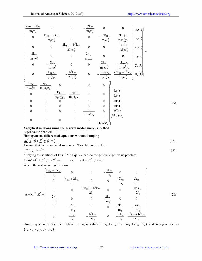
Using equation 3 one can obtain 12 eigen values ),,,,,( 654321 and 6 eigen vectors
),,,,,( 654321 x x x x x x
.
Journal of American Science, 2012;8(3) http://www.americanscience.org
http://www.americanscience.org [email protected] 576
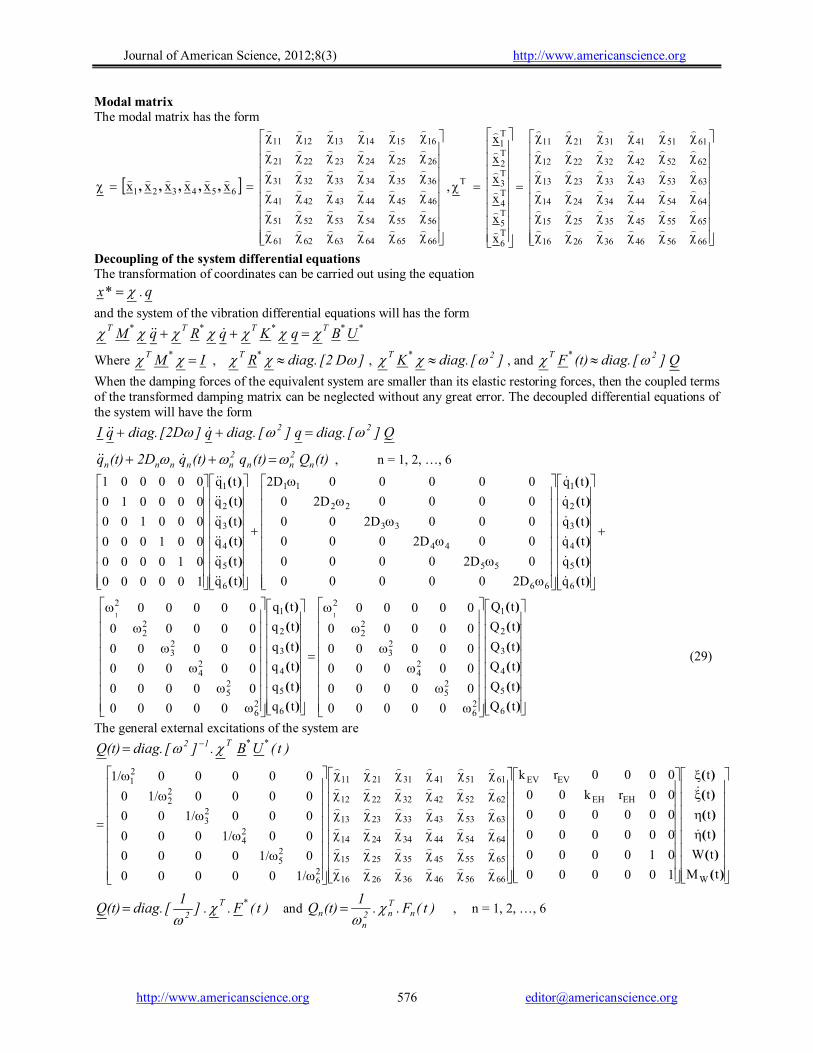
Modal matrix The modal matrix has the form
666564636261
565554535251
464544434241
363534333231
262524232221
161514131211
654321 x x x x x x
,,,,, ,
665646362616
655545352515
645444342414
635343332313
625242322212
615141312111
T6
T5
T4
T3
T2
T1
T
x
x
x
x
x
x
Decoupling of the system differential equations The transformation of coordinates can be carried out using the equation
q . *x
and the system of the vibration differential equations will has the form
UB q K q R q M**T*T*T*T
Where I M*T
, ]D [2 diag. R*T , ][ diag. K 2*T , and Q] [ diag. (t)F 2*T
When the damping forces of the equivalent system are smaller than its elastic restoring forces, then the coupled terms of the transformed damping matrix can be neglected without any great error. The decoupled differential equations of the system will have the form
Q ][ diag. q ][ diag. q] [2D diag. q I 22
(t)Q (t)q (t)q 2D (t)q n2nn
2nnnnn , n = 1, 2, …, 6
tq
tq
tq
tq
tq
tq
2D00000
02D0000
002D000
0002D00
00002D0
000002D
tq
tq
tq
tq
tq
tq
100000
010000
001000
000100
000010
000001
6
5
4
3
2
1
66
55
44
33
22
11
6
5
4
3
2
1
)(
)(
)(
)(
)(
)(
)(
)(
)(
)(
)(
)(
tQ
tQ
tQ
tQ
tQ
tQ
00000
00000
00000
00000
00000
00000
tq
tq
tq
tq
tq
tq
00000
00000
00000
00000
00000
00000
6
5
4
3
2
1
26
25
24
23
22
2
6
5
4
3
2
1
26
25
24
23
22
211
)(
)(
)(
)(
)(
)(
)(
)(
)(
)(
)(
)(
(29)
The general external excitations of the system are
)t(UB .][ diag. (t)Q**T12
)(
)(
)(
)(
)(
)(
tM
tW
t
t
t
t
100000
010000
000000
000000
00rk00
0000rk
1/00000
01/0000
001/000
0001/00
00001/0
000001/
W
EHEH
EVEV
665646362616
655545352515
645444342414
635343332313
625242322212
615141312111
26
25
24
23
22
21
)t(F . . ]1
[ diag. (t)Q*T
2
and )t(F . .
1 (t)Q n
Tn2
n
n
, n = 1, 2, …, 6
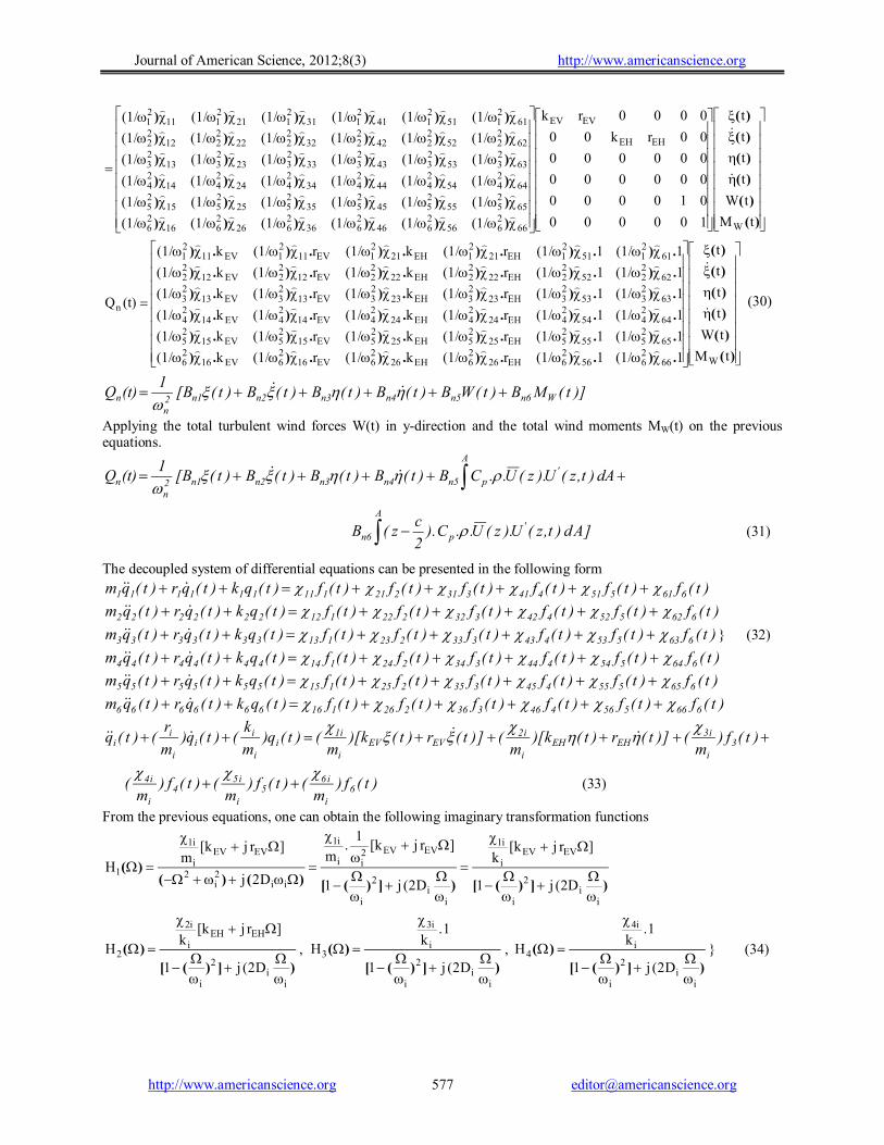
Journal of American Science, 2012;8(3) http://www.americanscience.org
http://www.americanscience.org [email protected] 577
)(
)(
)(
)(
)(
)(
))))))
))))))
))))))
))))))
))))))
))))))
tM
tW
t
t
t
t
100000
010000
000000
000000
00rk00
0000rk
(1/(1/(1/(1/(1/(1/
(1/(1/(1/(1/(1/(1/
(1/(1/(1/(1/(1/(1/
(1/(1/(1/(1/(1/(1/
(1/(1/(1/(1/(1/(1/
(1/(1/(1/(1/(1/(1/
W
EHEH
EVEV
662656
2646
2636
2626
2616
26
652555
2545
2535
2525
2515
25
642454
2444
2434
2424
2414
24
632353
2343
2333
2323
2313
23
622252
2242
2232
2222
2212
22
612151
2141
2131
2121
2111
21
)(
)(
)(
)(
)(
)(
.).).).).).)
.).).).).).)
.).).).).).)
.).).).).).)
.).).).).).)
.).).).).).)
tM
tW
t
t
t
t
1(1/1(1/r(1/k(1/r(1/k(1/
1(1/1(1/r(1/k(1/r(1/k(1/
1(1/1(1/r(1/k(1/r(1/k(1/
1(1/1(1/r(1/k(1/r(1/k(1/
1(1/1(1/r(1/k(1/r(1/k(1/
1(1/1(1/r(1/k(1/r(1/k(1/
(t)Q
W662656
26EH26
26EH26
26EV16
26EV16
26
652555
25EH25
25EH25
25EV15
25EV15
25
642454
24EH24
24EH24
24EV14
24EV14
24
632353
23EH23
23EH23
23EV13
23EV13
23
622252
22EH22
22EH22
22EV12
22EV12
22
612151
21EH21
21EH21
21EV11
21EV11
21
n
(30)
)]t(MB )t(WB )t(B )t(B )t(B )t([B 1
(t)Q Wn6n5n4n3n2n12n
n
Applying the total turbulent wind forces W(t) in y-direction and the total wind moments MW(t) on the previous equations.
dA )t,z(U).z(U..CB )t(B )t(B )t(B )t([B 1
(t)QA
'pn5n4n3n2n12
nn
]Ad )t,z(U).z(U..C ).2
cz(B
A'
pn6 (31)
The decoupled system of differential equations can be presented in the following form
)t(f)t(f)t(f)t(f)t(f)t(f)t(qk)t(qr)t(qm 661551441331221111111111
)t(f)t(f)t(f)t(f)t(f)t(f)t(qk)t(qr)t(qm 662552442332222112222222
)t(f)t(f)t(f)t(f)t(f)t(f)t(qk)t(qr)t(qm 663553443333223113333333 } (32)
)t(f)t(f)t(f)t(f)t(f)t(f)t(qk)t(qr)t(qm 664554444334224114444444
)t(f)t(f)t(f)t(f)t(f)t(f)t(qk)t(qr)t(qm 665555445335225115555555
)t(f)t(f)t(f)t(f)t(f)t(f)t(qk)t(qr)t(qm 666556446336226116666666
)t(f)m
(])t(r )t([k)m
(])t(r )t([k)m
()t(q)m
k()t(q)
m
r()t(q 3
i
i3EHEH
i
i2EVEV
i
i1i
i
ii
i
ii
)t(f)m
()t(f)m
()t(f)m
( 6i
i65
i
i54
i
i4 (33)
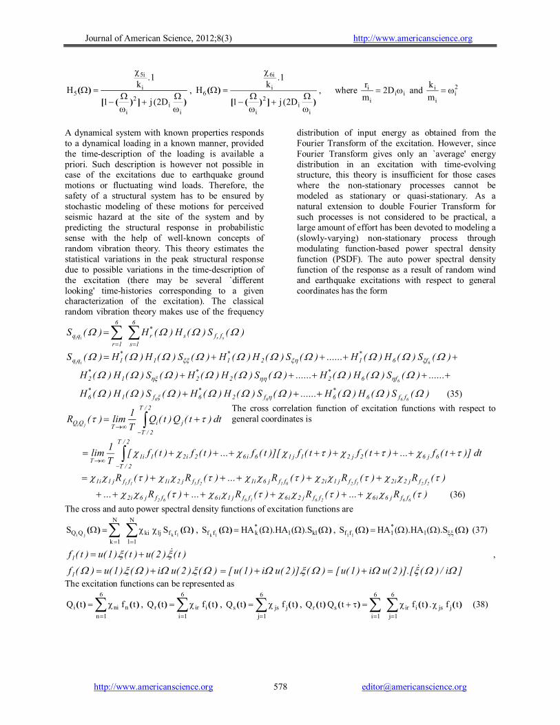
From the previous equations, one can obtain the following imaginary transformation functions
)])([)])([)()()(
ii
2
i
EVEVi
1i
ii
2
i
EVEV2ii
1i
ii2i
2
EVEVi
1i
1
D2( j1
]r j[kk
D2( j1
]r j[k1
.m
D2 j
]r j[km
H
)])([
)(
ii
2
i
EHEHi
2i
2
D2( j1
]r j[kk
H
,
)])([
)(
ii
2
i
i
3i
3
D2( j1
1 .k
H
,
)])([
)(
ii
2
i
i
4i
4
D2( j1
1 .k
H
} (34)
Journal of American Science, 2012;8(3) http://www.americanscience.org
http://www.americanscience.org [email protected] 578
)])([
)(
ii
2
i
i
5i
5
D2( j1
1 .k
H
,
)])([
)(
ii
2
i
i
6i
6
D2( j1
1 .k
H
, where iii
i D2m
r and 2
ii
i
m
k
A dynamical system with known properties responds to a dynamical loading in a known manner, provided the time-description of the loading is available a priori. Such description is however not possible in case of the excitations due to earthquake ground motions or fluctuating wind loads. Therefore, the safety of a structural system has to be ensured by stochastic modeling of these motions for perceived seismic hazard at the site of the system and by predicting the structural response in probabilistic sense with the help of well-known concepts of random vibration theory. This theory estimates the statistical variations in the peak structural response due to possible variations in the time-description of the excitation (there may be several `different looking' time-histories corresponding to a given characterization of the excitation). The classical random vibration theory makes use of the frequency
distribution of input energy as obtained from the Fourier Transform of the excitation. However, since Fourier Transform gives only an `average' energy distribution in an excitation with time-evolving structure, this theory is insufficient for those cases where the non-stationary processes cannot be modeled as stationary or quasi-stationary. As a natural extension to double Fourier Transform for such processes is not considered to be practical, a large amount of effort has been devoted to modeling a (slowly-varying) non-stationary process through modulating function-based power spectral density function (PSDF). The auto power spectral density function of the response as a result of random wind and earthquake excitations with respect to general coordinates has the form
6
1s
ffs*r
6
1r
qq )( S)(H )(H )(Ssrii
)( S)(H )(H......)( S)(H )(H)( S)(H )(H )(S6ii f6
*12
*11
*1qq
......)( S)(H )(H......)( S)(H )(H)( S)(H )(H6f6
*22
*21
*2
)( S)(H )(H......)( S)(H )(H)( S)(H )(H6666 ff6
*6f2
*6f1
*6 (35)
The cross correlation function of excitation functions with respect to general coordinates is
2/T
2/T
6j62j21j16i62i21i1T
dt )]t(f...)t(f)t(f)][t(f...)t(f)t(f[T
1lim
)(R)(R)(R...)(R)(R 2212612111 ffj2i2ffj1i2ffj6i1ffj2i1ffj1i1
)(R...)(R)(R...)(R... 66261662 ffj6i6ffj2i6ffj1i6ffj6i2 (36)
The cross and auto power spectral density functions of excitation functions are
N
1l
ffljki
N
1k
QQ lkjiS S )()( , )()( lkl
*kff ).S().HA(HA S
lk, )()( ).S().HA(HA S l
*1ff l1
(37)
)t().2(u)t().1(u)t(f1 ,
)().2(u i)().1(u)(f1 ]i/)()].[2(u i)1(u[)()].2(u i)1(u[
The excitation functions can be represented as
6
1n
nnii tf tQ )()( ,
6
1i
iirr tf tQ )()( ,
6
1j
jjss tf tQ )()( ,
6
1j
jjsiir
6
1i
sr tf . tf tQ tQ )()()()( (38)
2/T
2/T
jiT
QQ dt )t(Q )t(QT
1lim )(R
ji

Journal of American Science, 2012;8(3) http://www.americanscience.org
http://www.americanscience.org [email protected] 579
)()(
)()(
)()()()(
)()()()(
.
),().(.).(
),().(.
)()(
)()(
.
)(
)(
)(
)(
)(
)(
.)()(
'
')()(
tw6u
tv5u
0
0
t4ut3u
t2ut1u
1
dA tzUzU.C 2
cz
dA tzUzU.C
0
0
trtk
trtk
1
tf
tf
tf
tf
tf
tf
1tQ
T
121
A
p
A
p
EHEH
EVEV
T
121
6
5
4
3
2
1
T
121
1
)(..)()(
tf1
tQT
222
2
, )(..)()(
tf1
tQT
323
3
, )(..)()(
tf1
tQT
424
4
, )(..)()(
tf1
tQT
525
5
, )(..)()(
tf1
tQT
626
6
(39)
The cross correlation function of excitations is
2/T
2/T
srT
QQ dt )t(Q )t(QT
1lim )(R
sr
2/T
2/T
T
)s(2s
T
)r(2r
Tdt )]t(f
1)].[t(f
1[
T
1lim
2/T
2/T
N
1i
N
1j
jijsir2s
2r
Tdt )t(f)t(f
11
T
1lim
2/T
2/T
jiT
N
1i
N
1jjsir2
s2r
dt )t(f)t(fT
1lim
11
2/T
2/T
jiT
N
1i
N
1jjsir2
s2r
dt )t(f)t(fT
1lim
11
)(R.
11
ji ff
N
1i
N
1jjsir2
s2r
)](R.)(R.)(R.)(R.)(R..[11
6656655511 ffs6r6ffs5r6ffs6r5ffs5r5ffs1r12
s2r
)](.)(..)(..)(.[.{ RrRkrRrkRk11
2EVEVEVEVEV
2EVs1r12
s2r
)]}(.)(.)(.)(.[66566555 66566555 ffsrffsrffsrffsr RRRR
The cross power spectral density function of excitation functions has the form
)](.)(..)(..)(.[.{11
)( 221122
SrSkrSrkSkS EVEVEVEVEVEVsr
sr
QQ sr
]})(X.)(X.)(X.)(X.)[(S).z(U..C2
22s6r6
2
21s5r6
2
12s6r5
2
11s5r5uu222
f
)(S.11
)(Sjisr ff
N
1i
N
1jjsir2
s2r
(40)
The differential equations of motion can be written in the form
)t(Q.)t(Q.m
1)t(q
m
k)t(q
m
R)t(q i
2i
'i
ii
i
ii
i
ii
)t(Q.)t(Q.k
1)t(Q.
k
1)t(q.)t(q.D2)t(q i
2i
'i
i
2i
'i
2i
ii
2iiiii with )t(Q.
m
11)t(Q '
ii
2i
i
(41)
The cross power spectral density function of the vibration response with respect to general coordinates is
)().S().H(H )(Ssrsr QQs
*rqq (42)
The cross power spectral density function of the vibration response with respect to original coordinates is
)(.S )(Sjisr qq
n
1j
sjri
n
1i
XX
(43)
Substitute from Eq. 42 in Eq. 46 results in
Journal of American Science, 2012;8(3) http://www.americanscience.org
http://www.americanscience.org [email protected] 580
)().S().H(.H )(Sjisr QQj
*i
n
1j
sjri
n
1i
XX
(44)
Substitute from Eq. 40 in Eq. 44, one can obtain the cross power spectral density function of the response with respect to original coordinates of the form
n
1l
ffljki
n
1k2jj
2ii
j*i
n
1j
sjri
n
1i
XX )(S.).1
.m
1().
1.
m
1).(().H(.H )(S
lksr
(45)
and the auto power spectral density function of the response with respect to original coordinates of the form
6
1s
ffsjri
6
1rjij
*i
6
1j
njni
6
1i
XX )(S.k
1.
k
1).().H(.H )(S
srnn (46)
The power spectral density function of the excitations Correlation function of the excitations The correlation function of the excitations with respect to general coordinates is
2/T
2/T
srT
QQ dt )t(Q )t(QT
1lim )(R
sr (47)
Substitute from Eq. 32 in Eq. 47 results in
2/T
2/T
A'
pr5r4r3r2r12r
TQQ dA )t,z(U).z(U..CB )t(B )t(B )t(B )t([B
1
T
1lim )(R
sr
)t(B )t(B )t([B 1
].Ad )t,z(U).z(U..C ).2
cz(B s3s2s12
s
A'
pr6
dt ]Ad )t,z(U).z(U..C ).2
cz(BdA )t,z(U).z(U..CB )t(B
A'
ps6
A'
ps5s4
2/T
2/T
s4r1s3r1s2r1s1r12s
2r
TQQ )t()t(BB )t()t(BB )t()t(BB )t()t(BB
11
T
1lim )(R
sr
Ad )t,z(U).z(U..C ).2
cz()t(BB dA )t,z(U).z(U..C)t(BB
A'
ps6r1
A'
ps5r1
)t()t(BB )t()t(BB )t()t(BB )t()t(BB s4r2s3r2s2r2s1r2
Ad )t,z(U).z(U..C ).2
cz()t(BB dA )t,z(U).z(U..C)t(BB
A'
ps6r2
A'
ps5r2
)t()t(BB )t()t(BB )t()t(BB )t()t(BB s4r3s3r3s2r3s1r3
Ad )t,z(U).z(U..C ).2
cz()t(BB dA )t,z(U).z(U..C)t(BB
A'
ps6r3
A'
ps5r3
)t()t(BB )t()t(BB )t()t(BB )t()t(BB s4r4s3r4s2r4s1r4
Ad )t,z(U).z(U..C ).2
cz()t(BB dA )t,z(U).z(U..C)t(BB
A'
ps6r4
A'
ps5r4
)t(].dA )t,z(U).z(U..C[BB )t(].dA )t,z(U).z(U..C[BBA
'ps2r5
A'
ps1r5

Journal of American Science, 2012;8(3) http://www.americanscience.org
http://www.americanscience.org [email protected] 581
)t(].dA )t,z(U).z(U..C[BB)t(].dA )t,z(U).z(U..C[BBA
'ps4r5
A'
ps3r5
]dA )t,z(U).z(U..C].[dA )t,z(U).z(U..C[BBA
'p
A'
ps5r5
]Ad )t,z(U).z(U..C ).2
cz(].[dA )t,z(U).z(U..C[BB
A'
p
A'
ps6r5
)t(].Ad )t,z(U).z(U..C ).2
cz([BB )t(].Ad )t,z(U).z(U..C ).
2
cz([BB
A'
ps2r6
A'
ps1r6
tAd tzUzU.C 2
czBB tAd tzUzU.C
2
czBB
A
ps4r6
A
ps3r6 )(].),().(.).([)(].),().(.).([ ''
]dA )t,z(U).z(U..C].[Ad )t,z(U).z(U..C ).2
cz([BB
A'
p
A'
ps5r6
dt ]Ad )t,z(U).z(U..C ).2
cz(].[Ad )t,z(U).z(U..C ).
2
cz([BB
A'
p
A'
ps6r6
)(RBB)(RBB )(RBB )(RBB 11
)(R s4r1s3r1s2r1s1r12s
2r
QQ sr
Ad )(R).z(U..C ).2
cz(BB dA )(R).z(U..CBB
A
Ups6r1
A
Ups5r1 ''
)(RBB )(RBB )(RBB )(RBB s4r2s3r2s2r2s1r2
Ad )(R).z(U..C ).2
cz(BB dA )(R).z(U..CBB
A
Ups6r2
A
Ups5r2 ''
)(R.BB)(RBB )(R.BB )(R.BB s4r3s3r3s2r3s1r3
Ad )(R).z(U..C ).2
cz(BB )dA(R ).z(U..CBB
A
Ups6r3
A
Ups5r3 ''
)(RBB )(RBB )(RBB )(RBB s4r4s3r4s2r4s1r4
Ad )(R).z(U..C ).2
cz(BB dA )(R).z(U..CBB
A
Ups6r4
A
Ups5r4 ''
A
Ups3r5
A
Ups2r5
A
Ups1r5 dA )(R).z(U..CBB dA )(R).z(U..CBB dA )(R).z(U..CBB '''
A
21UU2122
p
A
s5r5
A
Ups4r5 dA.).dA(R).z(U).z(U..CBBdA )(R).z(U..CBB '2
'1
'
Ad )(R).z(U..C ).2
cz(BB dA.).dA(R)
2
cz).(z(U).z(U..CBB
A
Ups1r6
A
21UU22122
p
A
s6r5 '
2
'2
'1
1

Journal of American Science, 2012;8(3) http://www.americanscience.org
http://www.americanscience.org [email protected] 582
Ad )(R).z(U..C ).2
cz(BBAd )(R).z(U..C ).
2
cz(BB
A
Ups3r6
A
Ups2r6 ''
2
'1
'2
1
'
A
21UU12122
p
A
s5r6
A
Ups4r6 dA.).dA(R).2
cz).(z(U).z(U..CBB Ad )(R).z(U..C ).
2
cz([BB
2
'2
'1
1 A
21UU2122
p21
A
s6r6 dA.).dA(R).z(U).z(U..C)2
cz)(
2
cz(BB (48)
Since the wind velocity U(z,t) and the underground excitations (t) ,t )( are uncorrelated, the following correlation
functions must have the values of zero.
0)(R)(R)(R)(R '''' UUUU
and 0)(R)(R)(R)(R '''' UUUU
(49)
The power spectral density function of the excitations The cross power spectral density function of the excitations with respect to general coordinates is
de )(R)}(RF{ )(S i-QQQQQQ srsrsr
(50)
Substitute from Eqs. 48 and 49 in Eq. 50 results in
)(RBB )(RBB )(RBB)(RBB )(RBB )(RBB 11
)(S s2r2s1r2s4r1s3r1s2r1s1r12s
2r
QQ sr
)(R.BB)(RBB )(R.BB )(R.BB )(RBB )(RBB s4r3s3r3s2r3s1r3s4r2s3r2
)(RBB )(RBB )(RBB )(RBB s4r4s3r4s2r4s1r4
A
21UU2122
p
A
s5r5 dA.).dA(R).z(U)z(U..CBB '2
'1
2
'2
'1
1 A
21UU22122
p
A
s6r5 dA.).dA(R)2
cz).(z(U)z(U..CBB
2
'2
'1
1 A
21UU2122
p1
A
s5r6 dA.).dA(R).z(U).z(U..C )2
cz(BB
de dA.).dA(R).z(U).z(U..C)2
cz)(
2
cz(BB i
A
21UU2122
p21
A
s6r6
2
'2
'1
1
SBB SBB SBBSBB SBB SBB 11
S s2r2s1r2s4r1s3r1s2r1s1r12s
2r
QQ sr)()()()()()()(
)(S.BB)(SBB )(S.BB )(S.BB )(SBB )(SBB s4r3s3r3s2r3s1r3s4r2s3r2
)(SBB )(SBB )(SBB )(SBB s4r4s3r4s2r4s1r4
A
21UU2122
p
A
s5r5 dA.).dA(S)z(U)z(U..CBB21
2
21
1 A
21UU22122
p
A
s6r5 dA.).dA(S)2
cz).(z(U)z(U..CBB
Journal of American Science, 2012;8(3) http://www.americanscience.org
http://www.americanscience.org [email protected] 583
2
21
1 A
21UU2122
p1
A
s5r6 dA.).dA(S).z(U).z(U..C )2
cz(BB
2
21
1 A
21UU2122
p21
A
s6r6 dA.).dA(S).z(U).z(U..C)2
cz)(
2
cz(BB (51)
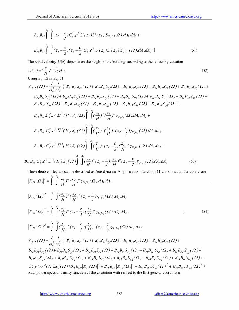
The wind velocity )(zU depends on the height of the building, according to the following equation
)H(U )H
z( )z(U (52)
Using Eq. 52 in Eq. 51
)(SBB )(SBB)(SBB )(SBB )(SBB 11
)(S s1r2s4r1s3r1s2r1s1r12s
2r
QQ sr
)(SBB )(S.BB )(S.BB )(SBB )(SBB )(SBB s3r3s2r3s1r3s4r2s3r2s2r2
)(SBB )(SBB )(SBB )(SBB )(S.BB s4r4s3r4s2r4s1r4s4r3
2
21
1 A
21UU21
A
U222
fs5r5 dA..dA)()H
z()
H
z()(S).H(U..C.BB
2
21
1 A
21UU221
A
U222
fs6r5 dA..dA)()2
cz()
H
z()
H
z()(S).H(U..C.BB
2
21
1 A
21UU2
11
A
U222
fs5r6 dA..dA)()H
z)(
2
cz()
H
z()(S).H(U..C.BB
2
21
1 A
21UU22
11
A
U222
fs6r6 dA..dA)()2
cz()
H
z)(
2
cz()
H
z()(S).H(U..C.BB
(53)
These double integrals can be described as Aerodynamic Amplification Functions (Transformation Functions) are
2
21
1 A
21UU21
A2
11 dA..dA)()H
z()
H
z()(X
,
2
21
1 A
21UU221
A2
12 dA..dA)()2
cz()
H
z()
H
z()(X
2
21
1 A
21UU2
11
A2
21 dA..dA)()H
z)(
2
cz()
H
z()(X
, } (54)
2
21
1 A
21UU22
11
A2
22 dA..dA)()2
cz()
H
z)(
2
cz()
H
z()(X
)(SBB)(SBB )(SBB )(SBB 11
)(S s4r1s3r1s2r1s1r12s
2r
QQ sr
)(S.BB )(S.BB )(SBB )(SBB )(SBB )(SBB s2r3s1r3s4r2s3r2s2r2s1r2
)(SBB )(SBB )(SBB )(SBB )(S.BB)(SBB s4r4s3r4s2r4s1r4s4r3s3r3
])(X.BB)(X.BB)(X.BB)(X.B[B )(S).H(U..C2
22s6r6
2
21s5r6
2
12s6r5
2
11s5r5U222
f
Auto power spectral density function of the excitation with respect to the first general coordinates

Journal of American Science, 2012;8(3) http://www.americanscience.org
http://www.americanscience.org [email protected] 584
)(SBB )(SBB )(SBB 11
)(S 13111211111121
21
QQ 11
)(SBB )(SBB )(SBB 121211121411
)(SBB )(S.BB )(S.BB )(SBB )(SBB 13131213111314121312
)(SBB )(SBB )(SBB )(SBB )(S.BB 14141314121411141413
2
121615
2
111515U222
f )(X.BB)(X.B[B )(S).H(U..C
])(X.BB)(X.BB2
221616
2
211516 (55)
Complex transformation matrix with respect to general coordinates Fourier transformation of the vibration response and excitation has the following form
)(Q . ] 2D i [- ).(q n2n
2nnn
2n
Where )(Q . )(H )(q nnn with ...,6 2, 1,n ,
)](2D[ i ])(-[1
1 )(H
nn
2
n
n
(56)
and its absolute value is ...,6 2, 1,n ,
)](D 2[ ])(-[1
1 )(AHF
2
nn
22
n
Response power spectral density function with respect to general coordinates Cross correlation functions of the response with respect to general coordinates have the form
d e )( S)(H )(H2
1 dt )t(q )t(q
T
1lim )(R i
QQs*r
2/T
2/T
srT
qq srsr (57)
The response power spectral density function with respect to general coordinates is
Cross: )}(RF{ )(Ssrsr qqqq and Auto: )(S .)(H )(S
nn Q
2
nq
Auto power spectral density function for n-eigen form with respect to general coordinates is
)(SBB )(SBB)(SBB )(SBB )(SBB 1
.)(H )(S n1n2n4n1n3n1n2n1n1n12n
2
nqq nn
)(S.BB )(S.BB )(SBB )(SBB )(SBB n2n3n1n3n4n2n3n2n2n2
)(SBB )(SBB )(SBB )(SBB )(S.BB)(SBB n4n4n3n4n2n4n1n4n4n3n3n3
])(X.BB)(X.BB)(X.BB)(X.B[B )(S).H(U..C2
22n6n6
2
21n5n6
2
12n6n5
2
11n5n5U222
f
} (58) Where the mechanical amplification functions (Transformation Functions) are
...,6 2, 1,n ,
)](2D[ i ])(-[1
1 )(H
2
nn
22
n
2
n
(59)
and the Aerodynamic Amplification Functions (Transformation Functions) are shown in Eqs. 54 Response power spectral density function with respect to original coordinates Cross correlation functions of the response with respect to original coordinates have the form
2/T
2/T
srT
XX dt )t(X )t(XT
1lim )(R
sr
2/T
2/T
ji
6
1j
sjri
6
1iT
dt )t(q )t(qT
1lim
Journal of American Science, 2012;8(3) http://www.americanscience.org
http://www.americanscience.org [email protected] 585
)(R dt )t(q )t(qT
1lim
jiqq
6
1j
sjri
6
1i
2/T
2/T
jiT
6
1j
sjri
6
1i
(60)
The response power spectral density function with respect to original coordinates is
Cross: )(S )}(RF{ )(Sjisrsr qq
6
1j
sjri
6
1i
XXXX
and Auto: )(S. )(Snn q
6
1j
njni
6
1i
X
(61)
)(SBB)(SBB )(SBB )(SBB 1
.)(H. )(S n4n1n3n1n2n1n1n14n
2
n
6
1j
njni
6
1i
XX nn
)(S.BB )(S.BB )(SBB )(SBB )(SBB)(SBB n2n3n1n3n4n2n3n2n2n2n1n2
)(SBB )(SBB )(SBB )(SBB )(S.BB)(SBB n4n4n3n4n2n4n1n4n4n3n3n3
])(X.BB)(X.BB)(X.BB)(X.B[B )(S).H(U..C2
22n6n6
2
21n5n6
2
12n6n5
2
11n5n5U222
f
(62)
Mean square value response with respect to original coordinates Mean square value of the random vibration response with respect to original coordinates can be written as
d )(S2
1)0(R
nnnn XXX2X
(63) Conclusions This paper outlines a mathematical model describing the vibrations of high-tower buildings and its foundations with general-type equivalent passive springs and dampers, rigid bodies, and some ideal constraints under the effect of randomly fluctuating wind loads and the excitation of earthquake ground motions. Two derivation methods of the equivalent system’s differential equations have been considered, namely D’alembert’s principle and Lagrange’s method, which verified the acceptability of the developed equations of motion. Following conclusions can be withdrawn :
The mathematical model with 6 degrees of freedom presented in the present paper can be used to investigate the effect of both wind and earthquakes loading.
Analytical solution of the free vibrations of tall building and its foundation using the general modal analysis method has been performed.
Analytical solution of forced vibrations of tall building and its foundation has been developed, through the correlation function (time domain) and the power spectral density function (frequency domain) of system response with respect to general and also original coordinates.
Without wind and earthquakes, structures – particularly large ones – would probably be a lot easier to design and cheaper.
Random vibrations of building’s foundation subjected to seismic excitations of earthquake ground motions and also randomly fluctuating wind pressure fields acting on a building surface are analyzed. Nomenclature Cp Aerodynamic pressure factor (-) E Kinetic energy of the system (J) Ed Soil dynamic modulus of elasticity (kp/m3) F1H, F1V Spring and damping forces at C or E in horizontal and vertical direction (kp) F2H, F2V Spring and damping forces at D or F in horizontal and vertical direction (kp) FEH, FEV Spring and damping forces at s1 in horizontal and vertical direction due to earthquake effect (kp) H(iΩ) imaginary transformation function (-) J1, J2 Mass moment of Inertia of foundation with its accompanied vibrated soil and tall building (kg.s2.m) JF, JS Mass moment of Inertia of foundation and accompanied vibrated soil with it (kg.s2.m) kEH, kEV Linear horizontal and vertical equivalent spring stiffness of earth (kp/m) kEK Rotational equivalent spring stiffness of earth (kp.m/rad) kH, kV Linear horizontal and vertical equivalent spring stiffness of building-foundation connection (kp/m) L Lagrangian function (-) m1, m2 Total mass of foundation with its accompanied vibrated soil (mF+ mS) and tall building (kg) mF, mS Foundation and Vibrating soil mass (kg) MW(t) Total turbulent wind moment as a function of time (kp.m)
Journal of American Science, 2012;8(3) http://www.americanscience.org
http://www.americanscience.org [email protected] 586
Kq General coordinates
and ,y ,z , ,y ,z *2
*2
*1
*1
*1
*2 (m, m, rad, m, m, rad)
)(Rji QQ Cross correlation function of
the excitations (m2)
)(R),(Rsrsr XXqq Cross correlation function of
response with respect to general and original coordinates (m2) Rayleigh’s dissipation function (kp.m/s) rb Vertical embedding damping constant : the damping constant of radiation (kp.s/m3) rEK Rotational equivalent damping coefficient of earth (kp.m.s/rad) rEH, rEV Linear horizontal and vertical equivalent damping coefficient of earth (kp.s/m) rH, rV Linear horizontal, vertical equivalent damping coefficient of building-foundation connection (kp.s/m) rS Damping coefficient of the elastic soil bed (kp.s/m3) s1, s2 Centre of gravity of the foundation and tall building (-)
)(S),(Ssrii qqqq Auto and cross power
spectral density function of response w.r.t. general coordinates (m2.s/rad)
)(S),(Ssrii QQQQ Auto and cross power
spectral density function of excitations (m2.s/rad)
)(S),(Ssrnn XXXX Auto and cross power
spectral density function of response w.r.t. original coordinates (m2.s/rad) t Time (s) TEK Spring and damping torques about s1 in rotational direction (kp.m) U Potential energy of the system (J)
)H(U Average wind velocity along the
building height H (m/s)
)t(U),t(U zy Random displacement excitation
of earthquake in horizontal and vertical direction (m)
)t,z(U Wind speed as a function of space and
time (m/s)
)z(U Constant part of wind speed as a
function of space (m/s)
)t,z(U' Turbulent part of wind speed as a
function of space and time (m/s)
SV Vertical wave velocity (m/s)
)t(W Total turbulent wind force in y*-
direction as a function of time (kp)
)t,z(W Wind load as a function of space and time
(kp)
)z(W Constant part of wind load as a function
of space (kp)
)t,z(W' Turbulent part of wind load as a
function of space and time (kp) x
Amplitude of exponential solution of
motion differential equations (m)
)t(z ),t(y *o
*o Displacement of point O in the
direction of axisz and y *o
*o (m)
)( ),(z ),(y ),( ),(z ),(y 222111
non- dimensional Displacements (-)
)( ),(z ),(y ),( ),(z ),(y '2
'2
'2
'1
'1
'1
non- dimensional velocities (-)
)( ),(z ),(y ),( ),(z ),(y "2
"2
"2
"1
"1
"1
non- dimensional accelerations (-)
)t(z),t(y *1
*1 Displacement of gravity centre s1 of
foundation in *1
*1 z and y - axis (m)
)t(z),t(y *2
*2 Displacement of gravity centre s2 of
high tower building in *2
*2 z and y - axis (m)
)t(z ),t(y *C
*C Displacement of point C in the
direction of axisz and y *C
*C (m)
)t(z ),t(y *C
*C Velocity of point C in the direction
of axisz and y *C
*C (m/s)
)t(z ),t(y *C
*C Acceleration of point C in the
direction of axisz and y *C
*C (m/s2)
)t(z ),t(y *D
*D
Displacement of point D in the
direction of axisz and y *D
*D (m)
)t(z ),t(y *D
*D Velocity of point D in the direction
of axisz and y *D
*D (m/s)
)t(z ),t(y *D
*D Acceleration of point D in the
direction of axisz and y *D
*D (m/s2)
)t(z ),t(y *E
*E Displacement of point E in
the direction of axisz and y *E
*E (m)
)t(z ),t(y *E
*E Velocity of point E in the direction
of axisz and y EE ** (m/s)
)t(z ),t(y *E
*E Acceleration of point E in the direction
of axisz and y *E
*E (m/s2)

Journal of American Science, 2012;8(3) http://www.americanscience.org
http://www.americanscience.org [email protected] 587
)t(z ),t(y *F
*F Displacement of point F in the
direction of axisz and y *F
*F (m)
)t(z ),t(y *F
*F Velocity of point F in the direction of
axisz and y *F
*F (m/s)
)(),( ** tz ty FF Acceleration of point F in the
direction of axisz and y *F
*F (m/s2)
Profile constant (-)
B Specific weight of the high tower
building (kp/m3)
21 and,, Density of air , foundation , and
high tower building respectively (kg/m3) non-dimensional time [-]
)t(*o , )t(*
1 , )t(*2 Angular displacements
about axisx and,x,x *2
*1
*o [rad]
)t(o , )(t1 , )t(2 non - dimensional
angular displacement about
axisx and,x,x *2
*1
*o [-]
References
[1]- Ahearn, E.B.(2010) ; "Reduction of wind-induced vibrations in high-mast light poles." M.S., University of Wyoming, 167 pages; AAT 1491655.
[2]- Antonyuk, E.Ya. and Timokhin, V.V. (2007) ; "Dynamic response of objects with shock-absorbers to seismic loads." International Applied Mechanics, Vol. 43, No. 12.
[3]- Auersch, L. (2008) ; "Dynamic stiffness of foundations on inhomogeneous soils for a realistic prediction of vertical building resonance." J. of Geotechnical and Geoenvironmental Engineering, ASCE.
[4]- Balendra, T., Koh, C.G., and Ho, Y.C. (1991) ; "Dynamic response of buildings due to trains in underground tunnels." Earthquake Eng. Struct. Dyn., 20(3), pp. 275–29.
[5]- Belakroum, R., Mai, T.H., Kadja, M. et al. (2008) ; "Numerical simulation of dynamic wind loads on rectangular tall buildings." Inter. Review of Mechanical Engineering (I. RE. M.E), Vol. 2, N. 6.
[6]- Clouteau, D., Arnst, M., and Al-Hussaini, T.M. et al. (2005) ; "Freefield vibrations due to dynamic loading on a tunnel embedded in a stratified medium." J. Sound Vib., 283(1–2), pp. 173–199.
[7]- Davoodi, M., Mahmud Abadi, M., and Hessan, M. (2008) ; "Modal identification of 1:2 scaled model of a 4-story steel structure by impulse excitation." Seismic Eng. Conf. Commemorating the 1908 Messina and Reggio Calabria Earthquake.
[8]- Degrande, G., Schevenels, M., Chatterjee, P. et al. (2006a) ; "Vibration due to a test train at variable
speeds in a deep bored tunnel embedded in London clay." J. Sound Vib., 293(3–5), pp. 626–644.
[9]- Degrande, G., Clouteau, D., Othman, R. et al. (2006b) ; "A numerical model for ground-borne vibrations from underground railway traffic based on a periodic finite element—Boundary element formulation." J. Sound Vib., 293(3–5), pp. 645–666.
[10]-Forrest, J. A., and Hunt, H. E. M. (2006a) ; "Ground vibration generated by trains in underground tunnels." J. Sound Vib., 294(4–5), pp. 706–736.
[11]-Ghafari Oskoei, S.A. (2011) ; "Earthquake-resistant design procedures for tall guyed telecommunication masts." Ph.D., McGill University (Canada), 235 pages; AAT NR74516.
[12]-Gong, Y. (2010) ; "A New free vibration analysis method for space mega frames of super tall buildings." Materials Science and Engineering 10, 012002 doi:10.1088/1757-899X/10/1/012002.
[13]-Gouasmia, A. and Djeghaba, K. (2009) ; "Direct approach to seismic soil-structure-interaction analysis: Building group case." Inter. Review of Mechanical Engineering (I.RE.M.E.), vol. 3, M. 5.
[14]-Gupta, S., Hussein, M., Degrande, G. et al. (2007) ; "A comparison of two numerical models for the prediction of vibrations from underground railway traffic." Soil Dyn. Earthquake Eng., 27(7), pp. 608–624.
[15]-Kim, S.J. (2008) ; "Seismic assessment of RC structures considering vertical ground motion." University of Illinois at Urbana-Champaign, ISBN: 9781109026320. [16]-Kliukas, R. Jaras, A., and Kacianauskas, R. (2008) ; Investigation of traffic-induced vibration in Vilnius Arch-Cathedral Belfry. Transport 23(4), pp. 323–329.
[17]-Krier, D. (2009) ; "Modeling of integral abutment bridges considering soil-structure interaction effects." The University of Oklahoma, ISBN: 9781109451252.
[18]-Kurzweil, L.G. (1979) ; "Ground-borne noise and vibration from underground rail systems." J. Sound Vib., 66(3), pp. 363–370.
[19]-Kuźniar, K. and Waszczyszyn, Z. (2006) ; "Neural networks and principal component analysis for identification of building natural periods." J. of Computing in Civil Engineering 20, ASCE, pp.431-436.
[20]-Lorenz, H. (1955) ; "Dynamik im Grundbau." Grundbau Taschenbuch, B.I. Berlin., pp. 205.
[21]-Melke, J. (1988) ; "Noise and vibration from underground railway lines : proposals for a prediction procedure." J. Sound Vib., 120(2), pp. 391–406.
[22]-Metrikine, A.V., and Vrouwenvelder, A. C. W. M. (2000) ; "Surface ground vibration due to moving

Journal of American Science, 2012;8(3) http://www.americanscience.org
http://www.americanscience.org [email protected] 588
train in a tunnel: Two-dimensional model." J. Sound Vib., 234(1), pp. 43–66.
[23]-Panagiotou, M.: Seismic design, testing and analysis of reinforced concrete wall buildings. University of California, San Diego, ISBN: 9780549561705, 2008.
[24]-Prowell, I.: An Experimental and Numerical Study of Wind Turbine Seismic Behavior. Ph.D., University of California, San Diego, 309 pages; AAT 3449912, 2011.
[25]-Shyu, R. J., et. al.: The characteristics of structural and ground vibration caused by the TRTS trains. Metro’s Impact on Urban Living, Proc., World Metro Symp., Taipei, Taiwan, 610, 2002.
[26]-Sonmez, E.: Deterministic and stochastic responses of smart variable stiffness and damping systems and smart tuned mass dampers. Ph.D., Rice University, 318 pages; AAT 3421186, 2010.
[27]-Soudkhah, M.: Development of engineering continuum models for seismic soil-foundation interaction. Ph.D., University of Colorado at Boulder, 676 pages; AAT 3433347, 2010.
[28]-Trochides,A.: Ground-borne vibrations in buildings near subways.Appl. Acoustics, 32, 1991, pp.289–296.
[29]-Turner, J.: Vibration isolation: Harmonic and seismic forcing using the Wilson Theta method. ASHRAE Transactions: Symposia, 2004.
[30]-Ulusoy, H.S.: Applications of System Identification in Structural Dynamics: A Realization Approach. Ph.D., University of California, Irvine, 119 pages; AAT 3444318, 2011.
[31]-Uzdin, A.M., Doronin, F.M., Davydova, G.V. et al. (2009) ; "Performance analysis of seismic-insulating kinematic foundations on support elements with negative stiffness." Soil Mechanics and Foundation Engineering, Vol. 46, No. 3.
[32]-Weng, S.: A new substructuring method for model updating of large-scale structures. Ph.D., Hong Kong Polytechnic University (Hong Kong), 319 pages; AAT 3448510, 2010.
[33]-Wieser, J. : Assessment of Floor Accelerations in Yielding Buildings. M.Sc., University of Nevada, Reno, 272 pages; AAT 1494267, 2011.
[34]-Vadillo, E. G., Herreros, J., and Walker, J. G.: Subjective reaction to structurally radiated sound from underground railways: Field studies. J. Sound Vib., 193(1), 1996, pp. 65–74.
[35]-Yang, Y.B. et al.: Soil vibrations caused by underground moving trains. J. of Geotechnical and Geoenvironmental Engineering, ASCE, 2008.
[36]-Yao, M.M.: Earthquake Wave-Soil-Structure Interaction Analysis of Tall Buildings. Ph.D., University of Victoria (Canada), 95 pages; AAT NR74121, 2010.
[37]-Yun, C. B. et al.: Analytical frequency dependent infinite elements for soil- structure interaction analysis in two-dimensional medium. Eng. Struct., 22(3), 2000, pp. 258–271.
[38]-Zhong, P.: Sensitivity of building response to variation in integration time step of response history analysis. M.S., University of California, Irvine, 70 pages; AAT 1490700, 2011.
APPENDIX
FFF V.m , Foundation weight gmW FF . ,
Lorenz, H. (1955) calculated the weight of the accompanied vibrating soil with the foundation using the equation
ton,ba8350AfW 3434FS
)/()/( ].].[.[. gWm SS /
kg.
SF1 mmm , 2SSS
2fFF1 lmJlmJJ .. ,
)]/([
]/)][(/[)(.
FS
FSF
F
SS
F
SF
mm1
2hdmml
2
hd
m
ml
m
m l
Fig. 4 Foundation with its accompanied vibrating
toned sand
SF
S
rA
W h
. , ]/)[( FS l2hdl ,
]12/)ed.[(mJ 22FF , ]/).[( 12ehmJ 22
SS
Vertical embedding damping constant: the damping
constant of radiation is Sdb VEr /
Mass of the high tower: the density of high tower can be assumed as 1/10 of that of the foundation, i.e.
10/12
g.m W, V.m 22222 , ]/).[( 12cbmJ 2222
2/25/12