journal of applicable chemistry · journal of applicable chemistry 2014, 3 (6): ... starting with a...
TRANSCRIPT

2209
Available online at www.joac.info
ISSN: 2278-1862
Journal of Applicable Chemistry 2014, 3 (6): 2209-2311
(International Peer Reviewed Journal)
State-of-Art-Review (SAR-Invited)
Mathematical Neural Network (MaNN) Models
Part VI: Single-layer perceptron [SLP] and Multi-layer perceptron [MLP]
Neural networks in ChEM- Lab
K. RamaKrishna1, V. Anantha Ramam
2, R. Sambasiva Rao
2*
1. Department of Chemistry, Gitam Institute of Science, Gitam University,Visakhapatnam 530 017, INDIA
2. School of Chemistry, Andhra University, Visakhapatnam 530 003, INDIA
Email: [email protected], [email protected]
Accepted on 9th November 2014
(Dedicated with profound respects to V Surya Prakasam, M.Sc. (Hons), A.E.S, former lecturer and Head of Dept. of
physics, S R R & C V R Govt. College, Vijayawada during his birth centenary celebrations)
ABSTRACT Multi-layer perceptron (MLP) NN deals with fully connected feed-forward-supervised NNs in which the flow of data is in the forward direction i.e. from input layer to output layer through hidden ones (IL
HL … OL). Each neuron in a layer is connected to all the other neurons in the succeeding layer. But,
the neurons within the layer are not connected. The data comprises of explanatory variables(x) and
response (y). In general $LP_NN (with $:0-, 1-, 2- and >2-hidden layers) represents I/O (or 0-LP), S(ingle)LP or 1-LP, 2-LP and M(ulti)LP. Starting with a single neuron, the popular ADALINE and
MEDALINE-NNs with illustrative examples like copying, 'AND' 'OR' Boolean gates are described in I/O
category. SLP_NN, the life of today's data driven NN paradigm with extensive applications in industry, research and defense has its origin in mid 1980s. It is the start of a new era of NN research, 25 years after
the death blow to linear-ANNs for their inability to explain even a simple XOR problem.
The imbibing character of SLP and its superiority are demonstrated with numerical and literature reports in classification, function approximation, pattern recognition etc. The new NNs emerged (based on input
type, TFs, accumulation operators) are complex-, quaternion-, fuzzy-, higher-order SLPs, retaining the
basic philosophy of SLP architecture. RBF is also a SLP with Kernel TFs in the hidden layer and recurrent NNs are with partial/complete backward connections. The output of hidden layer of SLP is a
transformed form of input into a new space generated through TFs. The applications of SLP and MLP are
multifold covering nook and corner of every discipline. Only typical select case studies are briefed engulfing chemistry/chemical engineering, medicine/pharmacy/biosciences, electrical/ mechanical/
computer engineering, robotics, forecast of forex and weather prediction/environment/pollution. Multi-
sensor hyphenated instruments generate tensorial data in chemical, environmental, pharmaceutical and
clinical laboratory tasks. Mostly, the same sets of algorithms are used in chemometrics, enviromentrics and medicinometrics (Chem) for tensor data sets (Chem_Tensor abbreviated as CT). The computational
activity is now accepted as laboratory experiments (thus CT-Lab), just the same way of wet and dry labs
of last century.

R. Sambasiva Rao et al Journal of Applicable Chemistry, 2014, 3 (6):2209-2311
2210
www. joac.info
SLP mimics PCA, non-linear PCA, ARMA and polynomials when suitable object function and architecture
are used. The posterior probability and Bayesian estimation are also derived from the output. The
evolution in architecture gave birth to dynamic architectures, Ito/Funahashi model, centroid based/adaptive/self-feed-back/cascade correlation MLPs. The selection/sub-sets of patterns, layer-wise
learning/pseudo-inverse/mixture-of-experts, dynamic learning, AdaBoost, batch-wise training are a few
noteworthy advances in training Ws. The incorporation of a priori-knowledge into MLP is a new
dimension. The modifications of basic back propagation (BP) algorithm used to train MLP_NN are extensive. The first-/second- order optimization methods and nature inspired algorithms like SAA, GA,
PSO, ABC, ACO and differential evolution increased quality of Ws. Inverse NNs based on SLP/MLP for
XOR and function approximation tasks are successfully dealt with. The cognitron, neocognitron, neural gas, spiking nets, complicated NNs mimicking (partial) biological functions, recent intelligent integration
of statistics and NNs (NeuralWorks® Predict) and hybrids with nature-inspired algorithms find a niche in
the annals of data driven information extraction.
Keywords: Multi-Layer Perceptron (MLP), Neural networks, Function approximation, Interpolation, Pattern recognition, Chemistry, Medicinometrics, Pharmaceutics, Technology, Pollution, multiple-classes.
______________________________________________________________________________
Contents Multi-Layer Perceptron (MLP)-NN
1. Introduction
Feed forward
supervised neural networks
2. Z(ero hidden) layer perceptron- ZLP_NN, (or IO_NNs)
McCulloch and Pitts (MP_NN)
ADALINE MADALINE
3. S(ingle hidden) layer perceptron- SLP_NN
Copying operation
with SLP
Function
approximation
4. M(ultiple hidden) layer perceptron MLP_NN
Neural gardening tools
5. Quantum-NN
6. Inverse SLP (Output Input (O/I) mapping)
Methods for
inversion
7. Applications.Inverse_FF_layered (XHL_NNs)
Inverse-XOR using
inverse_SLP

R. Sambasiva Rao et al Journal of Applicable Chemistry, 2014, 3 (6):2209-2311
2211
www. joac.info
Classification of two
categories with
curved boundary
Inversion of NNs for
real life tasks
Iris classification
Character (printed digit) recognition
Handwritten zip code
Drug discovery
Aerospace application using Inversion of
MLP_NN
Output performance of
sonar system
8. Applications.Feed_forward_layered NNs
Metrics
Classification
Automation of
Classification
Function approximation
Automatic Speech
recognition systems
Chemometri
cs
Dietetometrics
Technometrics
Envirometrics
Geometrics
Medicinometrics
Electric (power)
engineering
Robots
Communication
Commerce
9. Architecture Evolution in MLP_NN
Centroid based
MLP_NN

R. Sambasiva Rao et al Journal of Applicable Chemistry, 2014, 3 (6):2209-2311
2212
www. joac.info
Dynamic
architecture-2 (DA2-
)-MLP_NN Training
Combination of MLP_NNs
Deep neural networks
Hybrid methods
10. Activation (Trasfer) functions Evolution in MLP_NN
Higher order
neurons (
Quaternionic
11. Learning Evolution in MLP_NN
12. Training algorithms Evolution in MLP_NNs
13. Universal function approximation theorem
14. A priori knowledge of data structure and/or profiles
15. Emulation of standard statistical results by SLP_NNs
16. Distribution of information in NNs
17. Current state of MLP_NN in research mode (2014)
18. Future scope
Appendices
Appendix-1 An ant
(Artificial neuron -- Accumulation_operator Neuron
Transfer_function
Appendix-2 Salt
(State-of-the-Art-of learning/training)
INTRODUCTION Feed forward supervised neural networks
The neuron popular in connectionist model of the brain is the processing element in artificial neural networks (ANNs). Neural network consists of a bundle of inter connected neurons. Each neuron receives
input signals or patters. They are modulated by connection strengths and are accumulated in the confluence
operation. A transfer (activation) function operates on it resulting in the output. Neural networks are
broadly classified into self-organizing and supervised types based on the data containing only the explanatory (X) factors and X as well as response variables (y). The premise of a supervised NN-model

R. Sambasiva Rao et al Journal of Applicable Chemistry, 2014, 3 (6):2209-2311
2213
www. joac.info
of pattern recognition is the assumption of a (fundamental) relationship between output signals of the phenomenon and the explanatory input factors, although it is not known explicitly many a time. The
objective is to extract it, even if the model is approximate or isomorphous. The number of neurons,
nowadays called processing elements/units (PEs or PUs), in input and output layers are equal to the number of variables in X and y. Thus, the number of measurements/ observations/ patterns in X and Y
space result in matrices of size [NP, dimx] and [NP, dimy]. Each row of the matrix represents a data point
or pattern in NN terminology. The mapping or transformation of input to output is in the forward direction
and thus referred to as feed forward (FF-) NNs.
Modern NN designers opine the prior reports (ADALINE,
MEDALINE, Hopfield, Brain-state-in-
a-box (BSB), Willshaw-Vander-Maliburg approach) before the rebirth
of NNs can be deemed as
classical/historical NNs. Of course,
they gave birth to the present form or their modified versions. Professional
II, a software package incorporated
many of the historical ones for first level user/NN appreciators. In
continuation of our reviewing
architectural details of NNs and their
applications in interdisciplinary research [303-311, 313], the evolution
of MLP_NNs and revolutionary
progress in learning/ optimization methods for bench mark datasets and
real life tasks are described in this
review [1-393].
2. Z(ero hidden) layer perceptron-
ZLP_NN (or I/O NNs)
SAP (simple as possible) is a popular approach in microprocessors and computer technology for pedagogical purposes and finds room in neural
networks too. The simplest possible neural network ever dreamt consists of a single neuron (Fig. 1a). It
can do copying, negating (Table 1) and inverting operations successfully. It can be represented in
the traditional IO_NN using one neuron in each
layer (Fig. 1b).
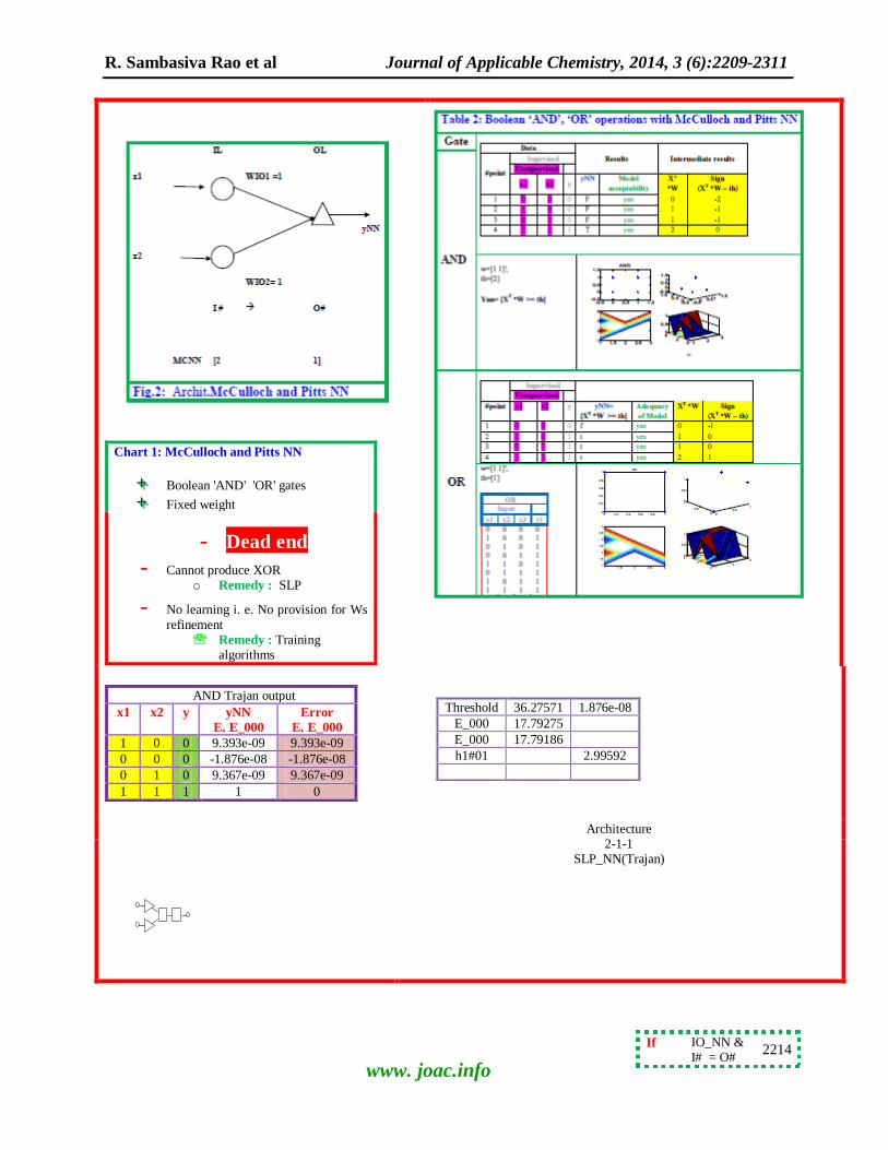
McCulloch and Pitts NN McCulloch-Pitts-neural network with fixed connection weight (i.e. no learning) models/
simulates/explains/mimics/emulates Boolean (and,
or) gates (Table 2, Fig. 2, chart 1). Here, X is the input, W is weight and yNN is output vectors of
NN. The response surface for three dimensional input is 4D- and thus, only numerical values are given.
The simple copying operation of MC neuron is illustrated in (Table A1-9a).
Table 1: Boolean Not operation
Boolean gate Data Weight, threshold
Not Gate
#point X y
1 0 1
2 1 0
w= [-1]
th=[0]
0 * (-1) = 0 ; 0 = threshold (0), hence fires i.e. y = 1
1 * (-1) = -1 ; -1 < threshold, hence does not fire i.e. y = 0
R. Sambasiva Rao et al Journal of Applicable Chemistry, 2014, 3 (6):2209-2311
2214
www. joac.info
Chart 1: McCulloch and Pitts NN
Boolean 'AND' 'OR' gates
Fixed weight
- Dead end
- Cannot produce XOR o Remedy : SLP
- No learning i. e. No provision for Ws
refinement Remedy : Training
algorithms
AND Trajan output
x1 x2 y yNN
E. E_000
Error
E. E_000
1 0 0 9.393e-09 9.393e-09
0 0 0 -1.876e-08 -1.876e-08
0 1 0 9.367e-09 9.367e-09
1 1 1 1 0
Threshold 36.27571 1.876e-08
E_000 17.79275
E_000 17.79186
h1#01 2.99592
Architecture 2-1-1
SLP_NN(Trajan)
If IO_NN & I# = O#

R. Sambasiva Rao et al Journal of Applicable Chemistry, 2014, 3 (6):2209-2311
2215
www. joac.info
Rosenblatt, in 1962 proposed input-output layer neural network (IO_NN) with linear learning rules as an excellent model for human brain. It is
also a simple architecture with parallel computation and efficient learning of
Boolean gates like ‗and‘, ‗or‘ etc. The advances in IO_NNs paved way to calculate eigen values, linear-PCs and dimension reduction of input space. The results of function approximation of tanh (y = tanh(x))
and linear (y =x) I/O mappings with TRAJAN software are given in table 3. Minsky and Papert showed
that this NN failed to classify XOR patterns.
Table 3a: Function approximation of tanh(x) with SLP_NN (1-1-1)
Y yNN Error
E_000 E_001 a2
T. a2 E. a2
-1.8 -0.946806 -0.946806 -2.889e-05
-1.6 -0.9217 -0.9217 4.906e-06
-1.4 -0.8854 -0.8854 2.485e-05
-1.2 -0.8337 -0.8337 2.569e-05
-1 -0.7616 -0.7616 -1.518e-05
-0.8 -0.664 -0.664 -1.022e-05
-0.6 -0.537 -0.537 -5.29e-06
-0.4 -0.379949 -0.379949 -1.114e-06
-0.2 -0.1974 -0.1974 1.652e-06
0 0 0 2.689e-06
0.2 0.1973753 0.1973753 2.262e-06
0.4 0.379949 0.379949 1.065e-06
0.6 0.5370496 0.5370496 -1.744e-07
0.8 0.6640368 0.6640368 -9.787e-07
1 0.7615942 0.7615942 -1.243e-06
1.2 0.8336546 0.8336546 -1.054e-06
1.4 0.8853517 0.8853517 -5.927e-07
1.6 0.9216686 0.9216686 -1.302e-08
1.8 0.946806 0.946806 5.639e-07
2.0 0.9640276 0.9640276 1.1e-06
-2 -1.5 -1 -0.5 0 0.5 1 1.5 2-1
-0.8
-0.6
-0.4
-0.2
0
0.2
0.4
0.6
0.8
1
%
% tanhsim.m 7/8/07
inc = 0.2;
[x]= [-1.8:inc:2]';
y = tanh(x) ;
figure,plot(x,y,'b.'),hold on
z = [x,y];save tanhsim.dat z -ascii
type tanhsim.dat
Table 3b: Function approximation with IO_NN using TRAJAN
(a) y=x ; x = [ 0 :0.1:1]’;
Chart 2: ADALINE
It functions as an adaptive FIR filter
with tapped input. The higher order transfer function can be obtained through z-transform
- Cannot solve XOR, since the
separating hyperplane is non-linear Remedy : SLP
Then Eigen values & PCs
R. Sambasiva Rao et al Journal of Applicable Chemistry, 2014, 3 (6):2209-2311
2216
www. joac.info
0 0 0.1 0.1
0.2 0.2 0.4 0.4 0.6 0.6 0.8 0.8 1 1
IO : [1-1]
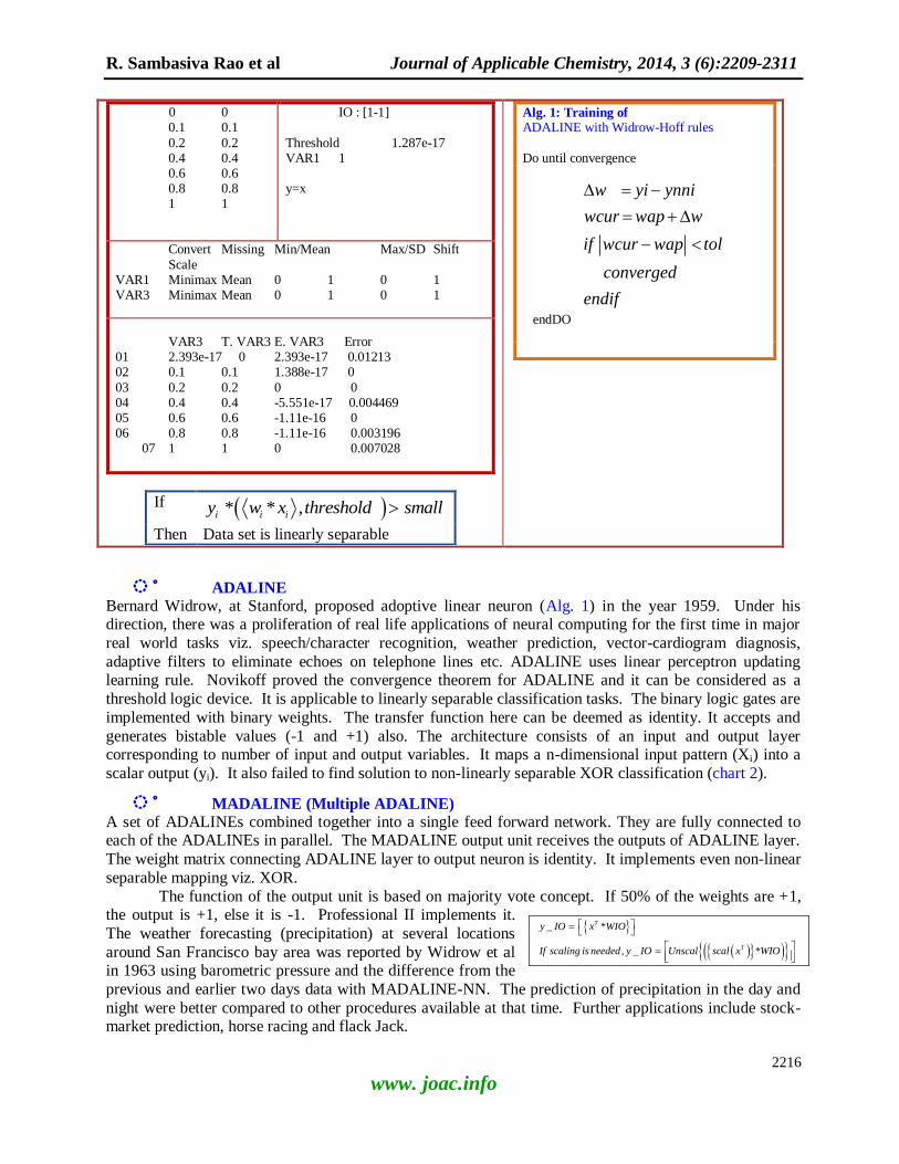
Threshold 1.287e-17 VAR1 1 y=x
Convert Missing Min/Mean Max/SD Shift
Scale VAR1 Minimax Mean 0 1 0 1 VAR3 Minimax Mean 0 1 0 1
VAR3 T. VAR3 E. VAR3 Error 01 2.393e-17 0 2.393e-17 0.01213 02 0.1 0.1 1.388e-17 0
03 0.2 0.2 0 0 04 0.4 0.4 -5.551e-17 0.004469 05 0.6 0.6 -1.11e-16 0 06 0.8 0.8 -1.11e-16 0.003196
07 1 1 0 0.007028
If * * ,i i iy w x threshold small
Then Data set is linearly separable
Alg. 1: Training of ADALINE with Widrow-Hoff rules
Do until convergence
w yi ynni
wcur wap w
if wcur wap tol
converged
endif
endDO
ADALINE Bernard Widrow, at Stanford, proposed adoptive linear neuron (Alg. 1) in the year 1959. Under his direction, there was a proliferation of real life applications of neural computing for the first time in major
real world tasks viz. speech/character recognition, weather prediction, vector-cardiogram diagnosis,
adaptive filters to eliminate echoes on telephone lines etc. ADALINE uses linear perceptron updating learning rule. Novikoff proved the convergence theorem for ADALINE and it can be considered as a
threshold logic device. It is applicable to linearly separable classification tasks. The binary logic gates are
implemented with binary weights. The transfer function here can be deemed as identity. It accepts and
generates bistable values (-1 and +1) also. The architecture consists of an input and output layer corresponding to number of input and output variables. It maps a n-dimensional input pattern (Xi) into a
scalar output (yi). It also failed to find solution to non-linearly separable XOR classification (chart 2).
MADALINE (Multiple ADALINE) A set of ADALINEs combined together into a single feed forward network. They are fully connected to each of the ADALINEs in parallel. The MADALINE output unit receives the outputs of ADALINE layer.
The weight matrix connecting ADALINE layer to output neuron is identity. It implements even non-linear
separable mapping viz. XOR.
The function of the output unit is based on majority vote concept. If 50% of the weights are +1, the output is +1, else it is -1. Professional II implements it.
The weather forecasting (precipitation) at several locations
around San Francisco bay area was reported by Widrow et al in 1963 using barometric pressure and the difference from the
previous and earlier two days data with MADALINE-NN. The prediction of precipitation in the day and
night were better compared to other procedures available at that time. Further applications include stock-market prediction, horse racing and flack Jack.
_ *
, _ *
T
T
y IO x WIO
If scaling is needed y IO Unscal scal x WIO
R. Sambasiva Rao et al Journal of Applicable Chemistry, 2014, 3 (6):2209-2311
2217
www. joac.info
3. S(ingle hidden) layer perceptron (SLP)-NN In 1986, Rumelhardt proposed a single hidden layer perceptron (SLP)-neural network (NN) affecting the
data flow from input, hidden to output layers. The layers are successively connected and there are no feedback or far off direct connections. Each unit in any layer has fan-in connections from all units in the
preceding (immediately below) and fan-out connections to all units in succeeding (immediately above)
layer. The word hidden is used as an end user is not interested in the details of operations in it. The strengths of connections are termed as weights (W) in analogy with synaptic strength in neurobiology. A
simple nonlinear (sigmoid) function is used as TF in the hidden layer. Further, it is neither a rule nor
exception of restricting a single transfer function in a PE and/or in each layer.
The weights (WIH, weight matrix of connections from input to hidden layer, WHO, weight matrix
of connections from hidden to output
layer) are learnt (refined) by back-propagation algorithm, which is
steepest gradient procedure tailor made
for on-line learning. A transformation of input with a non-linear (sigmoid) TF and back-propagation learning algorithm not only successfully implemented XOR gate, but has became a laudable architecture
for a reborn NN paradigm. It has only a little more intelligence in solving pattern recognition task. But,
SLP imbibes a galaxy of hither to available matured mathematical/statistical procedures. This paradigm
opened new vistas in non-collapsing learning of even odd data structures with unknown complex functional relationships. The input to output (I/O) mapping in NNs is affected by choosing architecture
(i.e. number of hidden layers, type of connections between neurons), TFs and training sets [19]. The
advantages of sigmoid TF in hidden layer are faster convergence, lower recognition error, and less sensitivity to learning parameters
Why a linear TF is preferable compared to nonlinear-TF in output layer? When the output layer of FF-MLP_NN uses a non-linear TF (like sigmoid), there arise more local minima
compared when a linear TF is employed. It was reported that re-constructive error surface for a sigmoidal
auto association consists of multiple local values compared to the linear one. When the weight vector of a
neuron reaches saturation area of a sigmoidal PEs, the derivative is zero. The error function for the final layer activation is nearly a flat region around this point. It is well known that the gradient techniques fail
to find the optima of such surfaces. In binary classification [18], the output values are in the range of zero
to one.
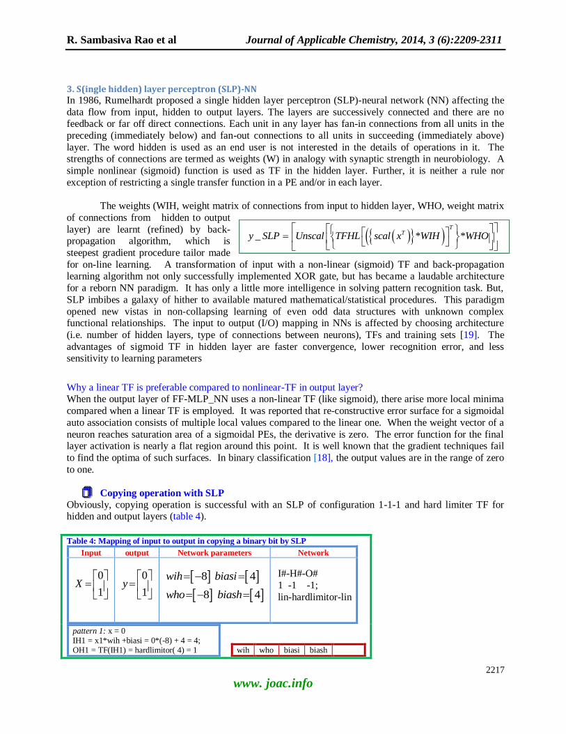
Copying operation with SLP
Obviously, copying operation is successful with an SLP of configuration 1-1-1 and hard limiter TF for hidden and output layers (table 4).
Table 4: Mapping of input to output in copying a binary bit by SLP
Input output Network parameters Network
0
1X
0
1y
8wih 4biasi
8who 4biash
I#-H#-O#
1 -1 -1;
lin-hardlimitor-lin
pattern 1: x = 0 IH1 = x1*wih +biasi = 0*(-8) + 4 = 4; OH1 = TF(IH1) = hardlimitor( 4) = 1
wih who biasi biash
_ * *T
Ty SLP Unscal TFHL scal x WIH WHO

R. Sambasiva Rao et al Journal of Applicable Chemistry, 2014, 3 (6):2209-2311
2218
www. joac.info
IO1 = OH1* who+ biash =1* (-8) +4 = -4;
OO = TFO(IO1) = hardlimitor(-4) =0 y = 0 ; yNN= OO; y-yNN = 0;
pattern 2: x = 1 IH1 = x1*wih +biasi = 1*(-8) + 4 = -4; OH1 = TF(IH1) = hardlimitor( -4) = 0 IO1 = OH1* who+ biash =0* (-8) +4 = 4; OO = TFO(IO1) = hardlimitor( 4) =1
y = 1 ; yNN= OO; y-yNN = 0;
-8 -8 4 4 Global
8 8 -4 -4 Global
-8 -8 0 0 Global
0.8 0.73 0 0 Local
Function approximation_SLP SLP_NN and in general NNs approximate functions, but the practical issue is the number of hidden neurons needed for a viable approximation. The simulated results for approximation of a quadratic
function (y = x2
) are detailed in application of NNs for modeling ozone [308]. The heuristics for function
approximation by NNs are in KB. 1 and function approximation of y = x is given in table 5.
Table 5: function approximation (y = x) by SLP
VAR3 T. VAR3 E. VAR3 Error
01 0.0 -0.031 0 -0.031 0.031 02 0.1 0.09627 0.1 -0.003729 0.003729 03 0.2 0.2225399 0.2 0.02254 0.02254 04 0.4 0.4608925 0.4 0.06089 0.06089 05 0.6 0.6662254 0.6 0.06623 0.06623 06 0.8 0.8302175 0.8 0.03022 0.03022
07 1.0 0.9534527 1 -0.04655 0.04655
Threshold 0.1445435 1.118388
VAR1 2.174794 h1#01 2.343879
lin-logistic-linear 1-1-1 SLP
Convert Missing Min/Mean Max/SD Shift Scale VAR1 Minimax Mean 0 1 0 1 VAR3 Minimax Mean 0 1 0 1
SLP
Polynomials approximated by SLP
- FF_NNs cannot model dynamic systems
Remedy: Recurrent-NNs
KB. 1: Heuristics for function approximation with
NNs
If SLP & TF is ridge function & Continuous almost everywhere &
Locally essentially bounded & Then SLP approximates any continuous
function with uniform norm
If SLP A1 &
TF : NonLinear A2 &
High number of neurons A3 & Then Approximates any function C1 If fn(x) is continuous in a closed
interval [a,b] &
fn(x) has M extrema &
Then SLP with M+1 sigmoid neurons approximates function
If polynomial with odd degree terms
Then TF : logistic sigmoid with null threshold
If polynomial with even degree terms Then TF : Gaussian
If TF is analytical & TF is non-polynomial Then fn approximation with
W as small as possible
If P(x) is a polynomial of degree p & TF has continuous derivatives
upto p+1 order
TF(x) 0 for 0<=I<=r
Then SLP approximates the polynomial & number of hidden neurons = & norm(p(x)-yNN) <=
R. Sambasiva Rao et al Journal of Applicable Chemistry, 2014, 3 (6):2209-2311
2219
www. joac.info
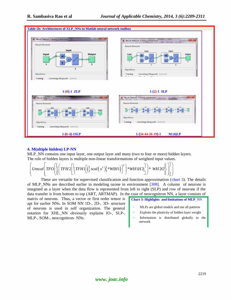
Table 5b: Architectures of XLP_NNs in Matlab neural network toolbox
1-[0]-1 ZLP 1-[2]-1 SLP
1-[6-4]-1SLP 1-[56-44-26-19]-1 M (4)LP
4. M(ultiple hidden) LP-NN
MLP_NN contains one input layer, one output layer and many (two to four or more) hidden layers.
The role of hidden layers is multiple non-linear transformations of weighted input values.
2 1 * 1 * 1 2 * 2T
TUnscal TFO TFH TFH scal x WIH WH H WH O
These are versatile for supervised classification and function approximation (chart 3). The details
of MLP_NNs are described earlier in modeling ozone in environment [308]. A column of neurons is imagined as a layer when the data flow is represented from left to right (SLP) and row of neurons if the
data transfer is from bottom to top (ART, ARTMAP). In the case of neocognitron NN, a layer consists of
matrix of neurons. Thus, a vector or first order tensor is apt for earlier NNs. In SOM NN 1D-, 2D-, 3D- structure
of neurons is used in self organization. The general
notation for XHL_NN obviously explains IO-, SLP-,
MLP-, SOM-, neocognitron- NNs.
Chart 3: Highlights and limitations of MLP_NN
MLPs are global models and use all patterns
Exploits the plasticity of hidden layer weight
Information is distributed globally in the network

R. Sambasiva Rao et al Journal of Applicable Chemistry, 2014, 3 (6):2209-2311
2220
www. joac.info
Neural gardening tools Using minimum error and/or maximum of performance
criteria, an optimum network is arrived. Yet, automatic selection of architecture of NN is still in a state of infancy.
Pruning methods, sensitivity analysis, information content
and data/goal accuracy/precision are instruments in the
hands of NN modeler. Recently, they are referred as neural gardening tools [14]. Karkkainen [18] performed
sensitivity analysis of FF-MLP_NN layer wise, comparing
different weight decay (linear, quadratic and convex) techniques. The object function is sum of Least Mean
Squares (LMS) and squares of Ws connecting. 5 Quantum NN A quantum NN basically works on quantum neuron [304]
and qubits. A Quant_NN exponentially gains speed over
classic neural networks through superposition of values entering and exiting a neuron (chart 4). Georgia Tech and
Oxford University also focus on futuristic systems. The
valid input to Qubit-NN is within the range 0 to 1. The
input neurons convert the numerical value into quantum
states in the range 0 to /2. It is passed through the hidden layer and output layer. The final output gives the
probability of the basic state of neuron. The training is
with quantum modified BP.
6. Inverse SLP (Output Input (O/I) mapping)
The word inverse is obvious as it is upside down of the original. The inversion of a matrix or trigonometric
function is well known. The product of a number/variable and its reciprocal is unity. Thus, the simplest reciprocal operator can also
be considered as an inverse operator. The inverse of a non-singular
square matrix is easily calculable. The product of it and its inverse is an identity matrix of same dimension (A * A
-1 = I). The near
singularity arises as a result of physical or numerical correlation.
Pseudo-inverse circumvents singularity problem by chopping off the dependent rows or columns. It is like
removing cancerous cells from healthy ones in an organ. The natural logarithm (loge) of an exponential (exp) of a number (x) is the number of itself [loge (exp(x)) x]. Similar instances are sin and sin
-1, and
differentiation and integration and so on.
It appears to be trivial even for simple processes like first order kinetics and some of the systems at
equilibrium. The transformation of A to B and back is a popular process in physical sciences. The latter
one B to A is an inverse of the forward process (A B). In biochemistry, physics and molecular biology,
simple mono-phasic to multi-phasic (more steps) processes involving multiple components are investigated with mathematical and experimental rigor. The mapping from output space to input space is
called inverse mapping. It is a locally ill posed problem as there is no unique solution. Further, it is
globally ill posed since there are multiple solution branches. Thus there is no closed form expression for the inverse mapping. Added to it, ill- conditioning increases as the complexity of the system grows. The
realizations for expected results in drug discovery are still a rosy dream of beauty and fragrance but also
with (inseparable) thorns.
- Weights (even in SLP) have no physical meaning
- Static i.e. time or space variation cannot modelled
- Greedy BP training settles in local minimum of
error surface
- Lack of localizability of Sigmoid TF
converges slowly
- Long training time
- Does not guarantee convergence of learning to
desired function
Remedy : RBF-NN
- Cannot account for higher order correlation
Remedy : Higher-order-NNs
- Learns noisy patterns also with increasing
number of hidden neurons
- Cannot handle discontinuities in input data
X $$_NN
Z(ero) 0 IO
S(ingle) 1 SLP
T(wo) 2 M(2)LP
M(ulti) 6 MLP
Chart 4: Advantages of Quantum NN
NN with a small number of neurons
is adequate
Reduction in the number of layers
Greater efficiency
R. Sambasiva Rao et al Journal of Applicable Chemistry, 2014, 3 (6):2209-2311
2221
www. joac.info
The prime objectives of inversion of neural networks are to detect generalization error and obtain
different network inversions for a given output data set. It enables one to explicitly express functional and
constraints on the network inversion. It paves way to probe into similar constrained optimization problems. Further, the relationship between network
inversion and parameters also can be thoroughly
examined for a successfully inverted NN (MLP or
RBF).
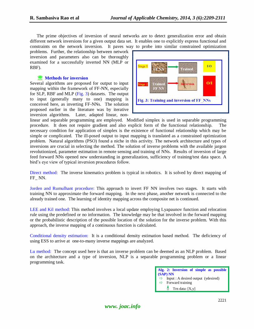
Methods for inversion
Several algorithms are proposed for output to input mapping within the framework of FF-NN, especially
for SLP, RBF and MLP (Fig. 3) datasets. The output
to input (generally many to one) mapping is conceived here, as inverting FF-NNs. The solution
proposed earlier in the literature was by iterative
inversion algorithms. Later, adapted linear, non-
linear and separable programming are employed. Modified simplex is used in separable programming procedure. It does not require gradient and also explicit form of the functional relationship. The
necessary condition for application of simplex is the existence of functional relationship which may be
simple or complicated. The ill-posed output to input mapping is translated as a constrained optimization problem. Natural algorithms (PSO) found a niche in this activity. The network architecture and types of
inversions are crucial in selecting the method. The solution of inverse problems with the available jargon
revolutionized, parameter estimation in remote sensing and training of NNs. Results of inversion of large
feed forward NNs opened new understanding in generalization, sufficiency of training/test data space. A bird‘s eye view of typical inversion procedures follow.
Direct method: The inverse kinematics problem is typical in robotics. It is solved by direct mapping of FF_ NN.
Jorden and Rumulhant procedure: This approach to invert FF NN involves two stages. It starts with training NN to approximate the forward mapping. In the next phase, another network is connected to the
already trained one. The learning of identity mapping across the composite net is continued.
LEE and Kil method: This method involves a local update employing Lyapaunov function and relocation rule using the predefined or no information. The knowledge may be that involved in the forward mapping
or the probabilistic description of the possible location of the solution for the inverse problem. With this
approach, the inverse mapping of a continuous function is calculated.
Conditional density estimation: It is a conditional density estimation based method. The deficiency of
using ESS to arrive at one-to-many inverse mappings are analyzed.
Lu method: The concept used here is that an inverse problem can be deemed as an NLP problem. Based
on the architecture and a type of inversion, NLP is a separable programming problem or a linear
programming task.
Alg. 2: Inversion of simple as possible
(SAP) NN
Input : A desired output (ydesired)
Forward training
Trn data: [X,y]

R. Sambasiva Rao et al Journal of Applicable Chemistry, 2014, 3 (6):2209-2311
2222
www. joac.info
Modified Simplex: Inversion of NLP or RBF is performed and
applied to a separable programming problem.
Inversion of MLP: A set of input patterns which produce a target output pattern are to be found (Alg. 2). The steepest descent
algorithm affects the minimization of the cost function. Inversion
of MLP or RBF is possible with separable programming method.
It is possible to invert NNs including prob_NN with differentiable activation functions.
7. Applications.Inverse_FF_layered (XHL_NNs)
Inverse-XOR using inverse_SLP
A 2D-binary XOR problem consists of two inputs x1 and x2 each with either one or zero. The output is 1
for heterogeneous input (x1+x2 = 1), while it is zero for homogeneous data (x1+x2 = 0 or x1+x2 = 2). The inverse problem is to find out x1 and x2 for a
known value of ytest. It is solved by two
approaches viz. inversion of MLP_NN and inversion of RBF-NN.
Inversion of SLP_NN: A SLP_NN with
architecture 2-2-1 was trained with BP. The inversion of MLP for the output 0.9 (ytest)
was performed with Imin and Imax
procedures by converting I to O mapping of MLP as a constrained NLP. The x1_invMLP,
x2_invMLP (input) obtained are well within
the acceptable limits. The sigmoid function
was approximated over the range -16 to +16 and the approximate LP was solved by
simplex procedure with restricted basis entry
rule. By increasing the number of grid points, errors will further be reduced.
The inversion of NN is performed
with gradient descent algorithm. The distribution of points on hyperplane depends
upon the basin of attraction. Thus, a break appears. In a separate experiment, SLP with bipolar inputs and
tanh TF is trained. The inversion with evolutionary algorithm results in a even distribution of points.
Hypinv is a pedagogical algorithm extracting rules from a trained NN in the form of hyperplane for continuous or binary inputs. Table 6 depicts the rules for XOR obtained by the inversion of NN.
Classification of two categories with curved boundary by inversion of SLP
Model : y = Fn(X; Ws,TF, AccOp)
Trn: (batch wise or point wise)
Estimate Reverse activity ( input vector) corresponding to desired output
Output : X_InvNN
Rule Base: If A1 ^ A2 ^ A3 ^ A4 ^ A5 ^ A6 ^ A7 then x2 where
A1 : −0.233x1 − 0.095x2 − 0.178 < 0 A2 : −0.336x1 + 0.276x2 − 0.305 < 0 A3 : +0.255x1 + 0.183x2 − 0.221 < 0 A4 : +0.038x1 − 0.121x2 − 0.091 < 0 A5 : −0.057x1 − 0.173x2 − 0.128 < 0

R. Sambasiva Rao et al Journal of Applicable Chemistry, 2014, 3 (6):2209-2311
2223
www. joac.info
Training and testing of 1000 samples each for a
two class problem with
points inside circle belonging to one class
and then outside to
another class are modeled
with 2-8-1 SLP_NN. HYPINV extracts the
most influential and
important variables first followed by less
important ones. It
approximates the discriminatory function with network decision boundaries using conjunction of 7 rules (chart 5)
Inversion of NNs for real life tasks
Inverse problems occur in electromagnetic surface design, flight control, vulnerability of large power
stations, snow parameters from passive microwave remote sensing measurements, kinematics, vibration
analysis etc. For that matter of fact, inversion is needed in each and every activity in animate and
inanimate life cycle of the universe in both space and time. Drug discovery and synthesis of materials of desired characteristics are vital inverse tasks. The available data and model are guidelines of retaining
influential variables in I O mapping. The difficulties in inverting each operation of the forward process
are not well explored area. With all these difficulties, still there are encouraging and noteworthy results in this decade.
Iris classification task - Inversion of SLP A SLP_NN of 4-3-2 architecture was trained with BP resulting in correct recognition rates of 100%, 93.3%
and 96.7% for setosa, versicolor and virginica. In this study the training set and test set comprise of 60 and
30 points for each class. The performance of the test data is acceptable as it is an interpolation task. The study of inversion of MLP_NN reported that extrapolation behavior of the system cannot be inferred based
only on test data within the interpolation region.
Character (printed digit) recognition_ inverse_SLP
The printed digits (i.e. integers 0 to 9) together with 540 noised patters are trained with SLP_NN (35-12-4). The input values obtained by NN-inversion for the digit '0', were fed to SLP_NN and the digit was
recognized as zero. But the naked eye could not decipher
some of the patterns.
Handwritten zip code – inverse_SLP From a database of 7291 training and 2007 test hand written
zip code characters (fig. 4), 500 patterns are used to train
SLP (256-30-4) with BP. Each input for NN consists of 16
x 16 pixels for a character. The correct recognition rates for 2007 and 6791 test samples are 78.1% and 82.9%
respectively. It appears that the performance of NN is
commendable. But, a peer inspection whether the test data set covers the entire input space or confined to a narrow
range (like a small patch) in a rectangular grid is important
to understand generalizability of NN model.
A6 : 0.268x1 − 0.108x2 − 0.199 < 0 A7 : 0.031x1 + 0.266x2 − 0.191 < 0. Simplification of extracted rules leads to If x2 > 0.83206 then negative class Else calculate rules
Chart 5: Extracted rules for two class task with curved boundary by inverse_SLP (Courtesy of E.W. Saad, D.C. Wunsch II, Neuralnetw., 20, 2007,78-93)
R. Sambasiva Rao et al Journal of Applicable Chemistry, 2014, 3 (6):2209-2311
2224
www. joac.info
Drug discovery
The experimental and simulated data available in pharmacy and mutagenicity is the start of invoking inverse models. In drug discovery for a best pharmaceutical product, the range of physical, chemical,
toxicological and biological variables are computable with today‘s available state of the art of inversion of
NNs. It iteratively improves the quality of the drug. Although inclusion of a priori knowledge is essential, traditional wisdom further complicates the situation. Inversion of this part is much more difficult at the
moment.
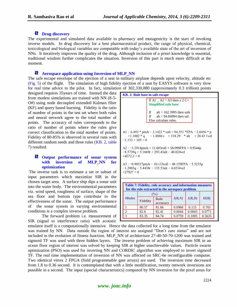
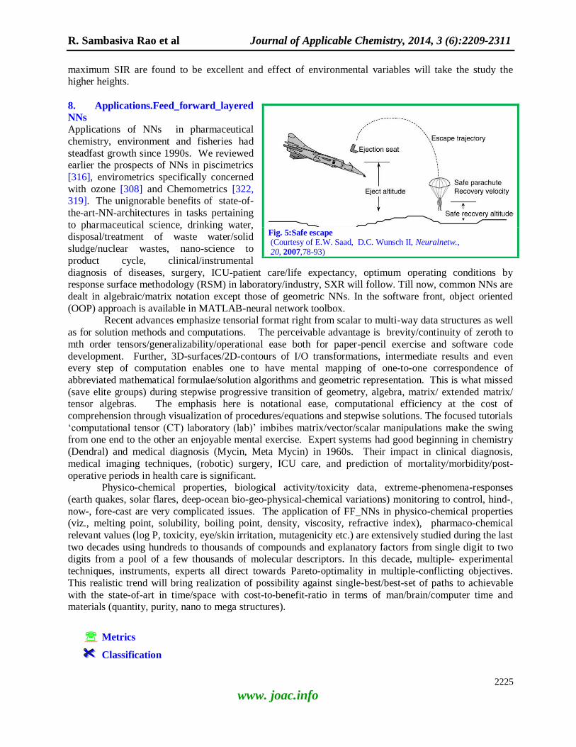
Aerospace application using Inversion of MLP_NN The safe escape envelope of the ejection of a seat in military airplane depends upon velocity, altitude etc
(Fig. 5) of the flight. The simulation of high fidelity ejection of a seat by EASYS software is very slow for real time advice to the pilot. In fact, simulation of 302,330,880 (approximately 0.3 trillion) points
designed requires 35years of time. Instead the data
from modest simulations are trained with NN (8-5-O#) using node decoupled extended Kalman filter
(KF) and query based learning. Fidelity is the ratio
of number of points in the test set where both rules and neural network agree to the total number of
points. The accuracy of rules corresponds to the
ratio of number of points where the rules give
correct classification to the total number of points. Fidelity of 80-85% is observed in several runs with
different random seeds and three rules (KB. 2, table
7) resulted.
Output performance of sonar system
with inversion of MLP_NN for
optimization The inverse task is to estimate a set or subset of
input parameters which maximize SIR in the chosen target area. A surface ship dips a sonar unit
into the water body. The environmental parameters
viz. wind speed, roughness of surface, shape of the sea floor and bottom type contribute to the
effectiveness of the sonar. The output performance
of the sonar system in varying environmental conditions is a complex inverse problem.
The forward problem i.e. measurement of
SIR (signal to interference ratio) with acoustic
emulator itself is a computationally intensive. Hence the data collected for a long time from the emulator was trained by NN. Data outside the region of interest are assigned ―Don‘t care status‖ and are not
included in the evolution of fitness function. MLP_NN of architecture 27-40-50-70-1200 was trained and
sigmoid TF was used with three hidden layers. The inverse problem of achieving maximum SIR in an ocean floor region of interest was solved by keeping SIR at higher unachievable values. Particle swarm
optimization (PSO) was used for inverting NN and CORDIC algorithm was employed to invert sigmoid
TF. The real time implementation of inversion of NN was affected on SRC-6e reconfigurable computer.
Two identical virtex 2 FPGA (field programmable gate arrays) are used. The inversion time decreased from 1.8 to 0.36 second. It is contemplated that with a little modification, twenty network inversions are
possible in a second. The input (special characteristics) computed by NN inversion for the pixel areas for
KB. 2: Rule base in safe escape
If A1 _ A2 ^ A3 then x 2 C+
Simplified rule base If alt > 162.3995 then safe
If alt < 94.84994 then saf. Else calculate rules.
A1 : 6.493 * pitch − 2.1422 * roll + 94.551 *FPA − 2.0456 * p +1.1002 * q − 1.8886 r + 318.29 * alt + 20.43 1vel −1.133 × 10⁵ > 0 A2 : −3.2914pitch + 11.603roll + 58.099FPA + 9.9544p −8.5739q + 5.1669r + 293.43alt − 40.824vel
+4572.2 > 0 A3 : −0.90337pitch − 10.133roll − 48.159FPA − 5.5235p −1.2003q − 5.4438r − 135.53alt − 4.6534vel +27927 < 0
Table 7: Fidelity, rule accuracy and information measures
for the rule extracted in the aerospace problem
#Rules
(%)
I(R,N) I(R,D) H(R) Fidelity
Rule
accuracy
1 80.57 81.66 0.0968 0.115 0.765
2 82.6 82.41 0.0044 0.0043 0.0771
3 83.35 84.74 0.0759 0.1005 0.5635
R. Sambasiva Rao et al Journal of Applicable Chemistry, 2014, 3 (6):2209-2311
2225
www. joac.info
maximum SIR are found to be excellent and effect of environmental variables will take the study the higher heights.
8. Applications.Feed_forward_layered
NNs
Applications of NNs in pharmaceutical
chemistry, environment and fisheries had
steadfast growth since 1990s. We reviewed earlier the prospects of NNs in piscimetrics
[316], envirometrics specifically concerned
with ozone [308] and Chemometrics [322, 319]. The unignorable benefits of state-of-
the-art-NN-architectures in tasks pertaining
to pharmaceutical science, drinking water, disposal/treatment of waste water/solid
sludge/nuclear wastes, nano-science to
product cycle, clinical/instrumental
diagnosis of diseases, surgery, ICU-patient care/life expectancy, optimum operating conditions by response surface methodology (RSM) in laboratory/industry, SXR will follow. Till now, common NNs are
dealt in algebraic/matrix notation except those of geometric NNs. In the software front, object oriented
(OOP) approach is available in MATLAB-neural network toolbox. Recent advances emphasize tensorial format right from scalar to multi-way data structures as well
as for solution methods and computations. The perceivable advantage is brevity/continuity of zeroth to
mth order tensors/generalizability/operational ease both for paper-pencil exercise and software code
development. Further, 3D-surfaces/2D-contours of I/O transformations, intermediate results and even every step of computation enables one to have mental mapping of one-to-one correspondence of
abbreviated mathematical formulae/solution algorithms and geometric representation. This is what missed
(save elite groups) during stepwise progressive transition of geometry, algebra, matrix/ extended matrix/ tensor algebras. The emphasis here is notational ease, computational efficiency at the cost of
comprehension through visualization of procedures/equations and stepwise solutions. The focused tutorials
‗computational tensor (CT) laboratory (lab)‘ imbibes matrix/vector/scalar manipulations make the swing from one end to the other an enjoyable mental exercise. Expert systems had good beginning in chemistry
(Dendral) and medical diagnosis (Mycin, Meta Mycin) in 1960s. Their impact in clinical diagnosis,
medical imaging techniques, (robotic) surgery, ICU care, and prediction of mortality/morbidity/post-
operative periods in health care is significant. Physico-chemical properties, biological activity/toxicity data, extreme-phenomena-responses
(earth quakes, solar flares, deep-ocean bio-geo-physical-chemical variations) monitoring to control, hind-,
now-, fore-cast are very complicated issues. The application of FF_NNs in physico-chemical properties (viz., melting point, solubility, boiling point, density, viscosity, refractive index), pharmaco-chemical
relevant values (log P, toxicity, eye/skin irritation, mutagenicity etc.) are extensively studied during the last
two decades using hundreds to thousands of compounds and explanatory factors from single digit to two digits from a pool of a few thousands of molecular descriptors. In this decade, multiple- experimental
techniques, instruments, experts all direct towards Pareto-optimality in multiple-conflicting objectives.
This realistic trend will bring realization of possibility against single-best/best-set of paths to achievable
with the state-of-art in time/space with cost-to-benefit-ratio in terms of man/brain/computer time and materials (quantity, purity, nano to mega structures).
Metrics
Classification
Fig. 5:Safe escape (Courtesy of E.W. Saad, D.C. Wunsch II, Neuralnetw., 20, 2007,78-93)
R. Sambasiva Rao et al Journal of Applicable Chemistry, 2014, 3 (6):2209-2311
2226
www. joac.info
A singleton cluster analysis is the simplest of the tasks with one class containing a single pattern. Binary classes comprising two clusters of different number of points/data structures/ distributions/ boundary
profile is a well-researched arena for over a century starting with simple Fisher linear discrimination
analysis to today‘s NNs through SVMs. Multiple classes in multiple-dimensions with correlated
features/ missing data/ complicated decision
boundaries drew special attention. Added to it, if
clusters exist in a hierarchical frame, the task becomes still complicated. Further, when a pattern belongs to
more than one class at each hierarchical level of the
tree, the consequence is that the task is NP hard. The sweet flavored and eye catching
adjectives are sometimes just used to uplift the results
like the word ‗state-of-the-art-$$$‘ with relatively simple data sets or comparing with already known
inferior methods over decades. The trust worthy
paradigms viz. computational intelligence, knowledge
based systems emerge only after several evolutions. But, combating with ill-effects, finding solutions for hurdles, incorporating best from the other domains, enhancing synergistic positive features, eliminating
negative aspects and/or limitations and at the same time retaining the best characteristics is a long journey.
In this attempt the basic philosophy of domain is safe guarded respectably.
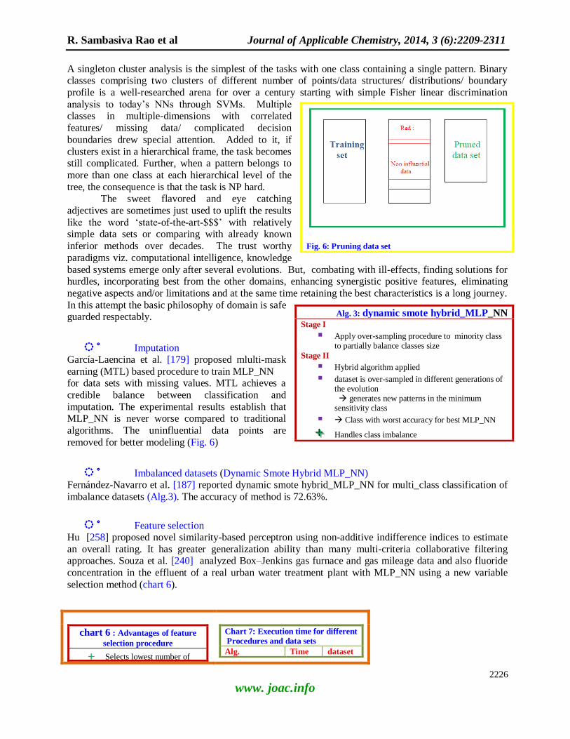
Imputation García-Laencina et al. [179] proposed mlulti-mask
earning (MTL) based procedure to train MLP_NN for data sets with missing values. MTL achieves a
credible balance between classification and
imputation. The experimental results establish that MLP_NN is never worse compared to traditional
algorithms. The uninfluential data points are
removed for better modeling (Fig. 6)
Imbalanced datasets (Dynamic Smote Hybrid MLP_NN)
Fernández-Navarro et al. [187] reported dynamic smote hybrid_MLP_NN for multi_class classification of
imbalance datasets (Alg.3). The accuracy of method is 72.63%.
Feature selection Hu [258] proposed novel similarity-based perceptron using non-additive indifference indices to estimate
an overall rating. It has greater generalization ability than many multi-criteria collaborative filtering approaches. Souza et al. [240] analyzed Box–Jenkins gas furnace and gas mileage data and also fluoride
concentration in the effluent of a real urban water treatment plant with MLP_NN using a new variable
selection method (chart 6).
chart 6 : Advantages of feature
selection procedure
Selects lowest number of
Chart 7: Execution time for different
Procedures and data sets
Alg. Time dataset
Fig. 6: Pruning data set
Alg. 3: dynamic smote hybrid_MLP_NN
Stage I
Apply over-sampling procedure to minority class to partially balance classes size
Stage II
Hybrid algorithm applied
dataset is over-sampled in different generations of the evolution generates new patterns in the minimum sensitivity class
Class with worst accuracy for best MLP_NN
Handles class imbalance
R. Sambasiva Rao et al Journal of Applicable Chemistry, 2014, 3 (6):2209-2311
2227
www. joac.info
variables and variable delays
Trained in one epoch
Low computational cost
Prospects in soft sensor
application
BP Back propagation EANNE Embedded ANN evolver
OBD Optimal Brain Damage OBDG OBD-based ANN
generation alg ReliefF Filter alg
WANNE Wapper ANN evolver
BPT
ReliefF
OBD
OBDG
few sec Iris
45 min. Madelon
WANNE 41 min Iris
70–80 h
Hardware Intel Core Duo 2.50 GHz processor 3 GB RAM
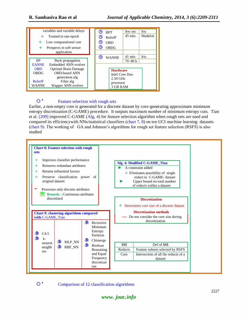
Feature selection with rough sets Earlier, a non-empty core is generated for a discrete dataset by core-generating approximate minimum entropy discretization (C-GAME) procedure. It outputs maximum number of minimum entropy cuts. Tian
et al. [209] improved C-GAME (Alg. 4) for feature selection algorithm when rough sets are used and
compared its efficiencywith NNs/statistical classifiers (chart 7, 8) on ten UCI machine learning datasets
(chart 9). The working of GA and Johnson‘s algorithms for rough set feature selection (RSFS) is also studied
Chart 8: Feature selection with rough
sets
Improves classifier performance
Removes redundant attributes
Retains influential factors
Preserve classification power of
original dataset
- Processes only discrete attributes
Remedy : Continuous attributes discretized
Alg. 4: Modified C-GAME_Tian
A constraint added
Eliminates possibility of single
reduct in C-GAME- dataset Upper bound on total number
of reducts within a dataset
Discretization
Determines core size of a discrete dataset
Discretization methods
Do not consider the core size during discretization
Chart 9: clustering algorithms compared with C-GAME_Tian
C4.5
k-
nearest neighbors
MLP_NN
RBF_NN
Recursive Minimum Entropy Partition
Chimerge
Boolean Reasoning and Equal Frequency
discretization
$$$ Def of $$$
Reducts Feature subsets selected by RSFS
Core Intersection of all the reducts of a
dataset
Comparison of 12 classification algorithms

R. Sambasiva Rao et al Journal of Applicable Chemistry, 2014, 3 (6):2209-2311
2228
www. joac.info
Fernández-Delgado,et al. [255] compared the functioning of 12 classification algorithms on 42 benchmark datasets including linear Direct Kernel
Perceptron (DKP). This procedure coded in C- and
Matlab is extremely efficient and has higher accuracy compared to more than 50% classifiers (chart 10). The
noteworthy feature is analytical closed form expression
is solved and requires only training patterns. The Ws in
the feature space minimize a combination of training error and hyperplane margin.
Bench mark data sets (MLP_NN + Biogeography-Based Optimization) Mirjalili et al. [205] trained MLP_NN with
Biogeography-Based Optimization (BioGeo
Based.Opt.) algorithm for classification (five datasets) as well as function approximation
(six data sets) tasks. A comparison with BP,
extreme learning machine (Extr.Lrn.Mach)
and heuristic algorithms showed that BioGeo Based.Opt. is competitive with
Extr.Lrn.Mach.
Chaos-based signals (MLP_NN + wavelet entropy)
Türk and Ogras [190] analysed 1806 CBDM
(chaos-based digital modulation) signals by
MLP_NN and wavelet entropy method with a classification rate of 98.76% (chart 11).
Classification of macro-invertebrates
Joutsijoki et al. [162] tested 13 algorithms to train MLP_NN for automatic
identification of eight different macroinvertebrates from1350 images (table 8). The
scaled conjugate gradient BP is the best training method for this task.
Hierarchical multi-label classification
In hierarchical multi-label classification, the classes are hierarchically arranged.
Each sample belongs to more than one class simultaneously in the same level as well as in hierarchy. Cerri et al. [220] proposed a new algorithm (Alg.5) and tested with several hierarchical multi-label classification
datasets. The results are better than those for two decision-tree induction methods. For many real life
tasks of this decade, modelling/prediction become a challenge even to arrive at Pareto optimality, leave alone an unique analytical global
optimal solution.
Automation of Classification Although evolutionary methods have been in use for feature selection,
structure design and training weights of NNs, there are only a few reports
on simultaneous evolution of whole classification/ function approximation task. Mostly, exploiting/ taking advantage at the same
Chart 10: Classifier algs.
MLP LDA Random Forest k-NN
RBF SVM Bagging of RPART decision trees
Generalised ART ELM
Adaboost
Chart 11a: Chaos-based
digital modulation
Chaos Shift Keying (CSK)
Chaotic On–Off Keying (COOK)
Differential Chaos Shift Keying (DCSK)
Correlation Delay Shift Keying (CDSK)
Symmetric Chaos Shift Keying (SCSK)
Frequency-Modulated Differential Chaos Shift Keying (FM-DCSK).
Wavelets
Daubechies,
Biorthogonal,
Coiflets,
Symlets wavelet
Chart 11b: Input and
models Input database
In vitro research
settings
Drug chemical
structure
Physico-chemical parameters
Models
MLP_NN (BP)
Neuro_fuzzy_ Mamdani MISO
Tfs : sigma, tanh
Tr : 447 records
Compounds:175
MLP_NN: I#-3-2-O# TF: sigma
Table 8: Comparision
of NNs in identification
of macroinvertebrates
NN %Accuracy
RBF 95.7
Prob 92.8
MLP 95.3
Alg. 5: Hierarchical multi-label
classification
Input For level =1: #levels_of_hierarchy
Trains MLP_NN
Input compute predicted values
End
output

R. Sambasiva Rao et al Journal of Applicable Chemistry, 2014, 3 (6):2209-2311
2229
www. joac.info
time respecting divide-and-conquer strategy has benefited in enhancing accuracy of solutions. Castellani [262] reported embedded approach is better than wrapper method (chart 12, KB.3) for 15 bench mark data
sets from UCI.
Function approximation Guo [11] introduced an adoptive FF-MLP_NN with no user defined parameters for function approximation
and pattern recognition. The number of neurons in each
hidden layer is equal to NP in the training set. It is like strict interpolation popular in RBF (SI-RBF) from the
point of view of number of neurons of the hidden layer.
But, Ws are estimated by matrix inner product and pseudo-inverse, which give exact solution. The
transmission of learning errors only in the forward
direction and layer wise training are the unique features. The procedure is automatic and requires only the desired
accuracy. The results show that it is faster than BP and
other gradient algorithms
Automatic Speech recognition systems
Automatic speech attribute transcription (ASAT) is
a lattice-based speech recognition system. Siniscalchi et al. [261] studied deep_NN with five to seven hidden
layers and each hidden layer containing up to 2048
neurons in classification accuracy task of phonetic
attributes (phonological features) and phonemes. The speaker-independent dataset of Wall Street Journal
corpus resulted in 90% accuracy. In automatic speech
recognition systems, MLP_NN derived acoustic features along with standard short-term spectral-based ones have
excelled in consistent performance. Park et al. [152]
introduced discriminative training approach on large training corpora. If the database is very large, multiple
individual MLPs are trained, each requiring shorter
amount of time, followed by combining the results of the
ensemble system. The test bed for this mega system is Arabic large vocabulary speech recognition. It includes
both conversation test data and news broadcasted.
Mirhassani and Ting [160] studied speech recognition task from utterances of six Malay vowels by 360
children of age between 7 and 12 years. The features are
extracted by fuzzy based discrimination method. It is better than Mel-frequency cepstral coefficient. MLP_NN and HMM are applied for speech recognition
with success. The weights of MLP_NN are trained by GA.
Chemometrics
CO2 absorption data in a packed absorption column: Shahsavand et al. [236] found RBF_NN performs
better than MLP_NN in filtering measurement noise in modeling CO2 absorption data in a packed absorption column. The pilot plant experiment was to separate CO2 from air at different concentrations
and rates of flow of methyl di-ethanolamine and di-ethanol amine (DEA).
KB. 3: Number of feature vs methods If Feature spaces are of small &medium size Then Evolutionary algorithms perform best &
reject redundant features effectively
If Feature correlations are preferable on under
sampled data Then Classical filter-based algorithms
If Large number of irrelevant features present Then Correlation- & saliency-based selection method
Chart 12: Evolutionary approach for whole
classification task
Wrapper approach
NN_structure
Input feature vector
training Ws
Embedded approach
Simultaneous Evolution of whole classifier
Datasets- Bench marks
Thirteen PR
Performance comparison
Methods Two manual
two automatic
Inference
Embedded >> Wrapper
Compactness of solution
Classification
Accuracy
Computational costs
R. Sambasiva Rao et al Journal of Applicable Chemistry, 2014, 3 (6):2209-2311
2230
www. joac.info
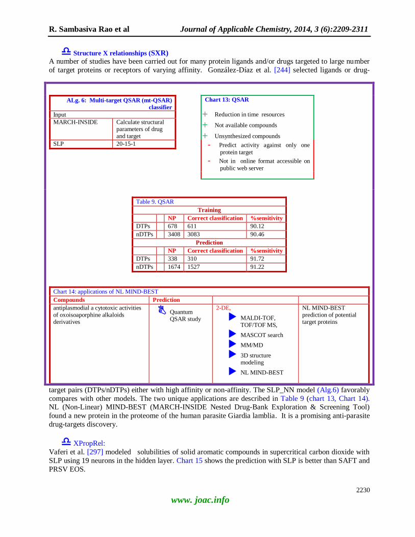
Structure X relationships (SXR) A number of studies have been carried out for many protein ligands and/or drugs targeted to large number
of target proteins or receptors of varying affinity. González-Díaz et al. [244] selected ligands or drug-
target pairs (DTPs/nDTPs) either with high affinity or non-affinity. The SLP_NN model (Alg.6) favorably
compares with other models. The two unique applications are described in Table 9 (chart 13, Chart 14). NL (Non-Linear) MIND-BEST (MARCH-INSIDE Nested Drug-Bank Exploration & Screening Tool)
found a new protein in the proteome of the human parasite Giardia lamblia. It is a promising anti-parasite
drug-targets discovery.
XPropRel:
Vaferi et al. [297] modeled solubilities of solid aromatic compounds in supercritical carbon dioxide with
SLP using 19 neurons in the hidden layer. Chart 15 shows the prediction with SLP is better than SAFT and
PRSV EOS.
ALg. 6: Multi-target QSAR (mt-QSAR)
classifier
Input
MARCH-INSIDE Calculate structural parameters of drug and target
SLP 20-15-1
Chart 13: QSAR
Reduction in time resources
Not available compounds
Unsynthesized compounds
- Predict activity against only one
protein target
- Not in online format accessible on
public web server
Table 9. QSAR
Training
NP Correct classification %sensitivity
DTPs 678 611 90.12
nDTPs 3408 3083 90.46
Prediction
NP Correct classification %sensitivity
DTPs 338 310 91.72
nDTPs 1674 1527 91.22
Chart 14: applications of NL MIND-BEST
Compounds Prediction
antiplasmodial a cytotoxic activities of oxoisoaporphine alkaloids derivatives
Quantum QSAR study
2-DE,
MALDI-TOF, TOF/TOF MS,
MASCOT search
MM/MD
3D structure modeling
NL MIND-BEST
NL MIND-BEST prediction of potential target proteins

R. Sambasiva Rao et al Journal of Applicable Chemistry, 2014, 3 (6):2209-2311
2231
www. joac.info
Solubility in supercritical carbon dioxide Lashkarbolooki et al. [199] developed predictive MLP_NN models for the solid solubilities of aromatic
hydrocarbons, aliphatic carboxylic acids, aromatic acids, heavy aliphatic and aromatic alcohols in the
supercritical carbon dioxide (table 10,11). The NN model is more accurate than Peng–Robinson (PR) and Soave–Redlich–Kwong (SRK) EOSs for the same compound set (chart 16).
Chart 15: solubilities in super critical CO2 by SLP
Experimental data published research reports
Input for
each solute
Temperature
Pressure
Critical properties
Acentric factor
Opt #HL neurons Minimum(.)
Absolute average relative deviation (AARD%)
Mean square error (MSE) Suitable regression coefficient (R2)
Archi-
tecture
I#-19-O#
TrnAlg: BP
Prediction
Method
Parameters
AARD%
SAFT
1 16.15
2 12.32%
3 7.65%
PRSV
EOS
21.10
Prediction of experimental data
AARD% 4.99
MSE 7.08 × 10⁻⁷
R2 0.99699
Table 10: Solubilities
by MLP_NN in
super critical CO2
AARD% 0.98
MSE 2.8 × 10⁻⁵
R2 0.9981
Table 11: Dataset
Tr
627
val 343
test 970
Prediction of percentage of oil, water and air: Roshani et al. [251] applied NN to predict precisely the
water, air and oil (chart 17) from measurements with a nuclear technique in annular multiphase regime.
Here, only one detector and a dual energy gamma-ray source are employed.
Material science
Chemical absorbents: Bastani et al. [196] employed MLP_NN for predicting CO2 loading capacity of chemical absorbents in a broad range of temperature, pressure and concentrations.
Smart materials: In the advanced technical applications, size, weight and performance of smart structures
is crucial. It poses a challenge for positioning actuators and sensors on smart gadgets in vibration controlled devices. The piezoelectric ceramics/ polymers based actuators excite only elastic modes of the
structures without disturbing rigid-body modes.
Piezoelectric actuators: Mehrabian et al. [243] reported an accurate way of arriving at location of
piezoelectric actuators for vibration suppression of flexible structures (chart 18). MLP_NNs along with
surface modeling and a stochastic invasive weed optimization algorithm adequately guided for a solution this complicated goal.
R. Sambasiva Rao et al Journal of Applicable Chemistry, 2014, 3 (6):2209-2311
2232
www. joac.info
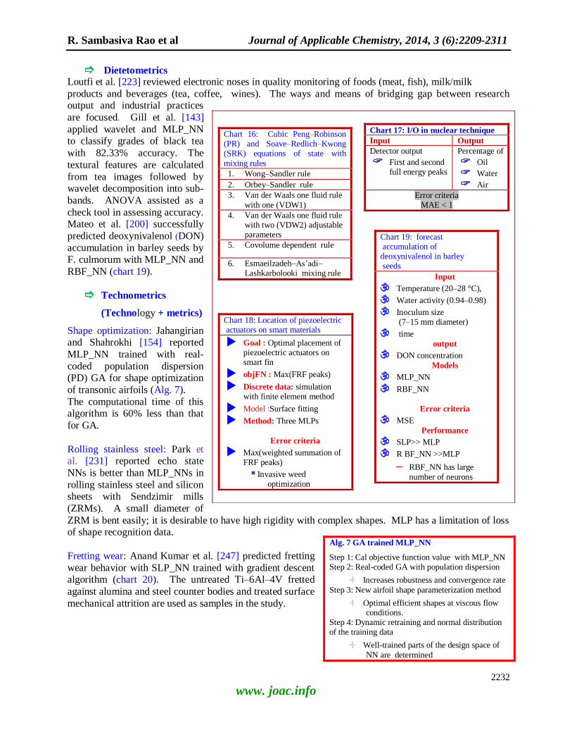
Dietetometrics Loutfi et al. [223] reviewed electronic noses in quality monitoring of foods (meat, fish), milk/milk
products and beverages (tea, coffee, wines). The ways and means of bridging gap between research output and industrial practices
are focused. Gill et al. [143]
applied wavelet and MLP_NN to classify grades of black tea
with 82.33% accuracy. The
textural features are calculated
from tea images followed by wavelet decomposition into sub-
bands. ANOVA assisted as a
check tool in assessing accuracy. Mateo et al. [200] successfully
predicted deoxynivalenol (DON)
accumulation in barley seeds by F. culmorum with MLP_NN and
RBF_NN (chart 19).
Technometrics
(Technology + metrics)
Shape optimization: Jahangirian and Shahrokhi [154] reported
MLP_NN trained with real-
coded population dispersion (PD) GA for shape optimization
of transonic airfoils (Alg. 7).
The computational time of this algorithm is 60% less than that
for GA.
Rolling stainless steel: Park et al. [231] reported echo state
NNs is better than MLP_NNs in
rolling stainless steel and silicon sheets with Sendzimir mills
(ZRMs). A small diameter of
ZRM is bent easily; it is desirable to have high rigidity with complex shapes. MLP has a limitation of loss of shape recognition data.
Fretting wear: Anand Kumar et al. [247] predicted fretting
wear behavior with SLP_NN trained with gradient descent algorithm (chart 20). The untreated Ti–6Al–4V fretted
against alumina and steel counter bodies and treated surface
mechanical attrition are used as samples in the study.
Chart 16: Cubic Peng–Robinson (PR) and Soave–Redlich–Kwong (SRK) equations of state with
mixing rules
1. Wong–Sandler rule
2. Orbey–Sandler rule
3. Van der Waals one fluid rule
with one (VDW1)
4. Van der Waals one fluid rule with two (VDW2) adjustable parameters
5. Covolume dependent rule
6. Esmaeilzadeh–As‘adi–Lashkarbolooki mixing rule
Chart 17: I/O in nuclear technique
Input Output
Detector output
First and second full energy peaks
Percentage of
Oil
Water
Air
Error criteria MAE < 1
Chart 19: forecast accumulation of deoxynivalenol in barley seeds
Input
Temperature (20–28 °C),
Water activity (0.94–0.98)
Inoculum size (7–15 mm diameter)
time
output
DON concentration
Models
MLP_NN
RBF_NN
Error criteria
MSE
Performance
SLP>> MLP
R BF_NN >>MLP
RBF_NN has large
number of neurons
Chart 18: Location of piezoelectric actuators on smart materials
Goal : Optimal placement of piezoelectric actuators on smart fin
objFN : Max(FRF peaks)
Discrete data: simulation with finite element method
Model :Surface fitting
Method: Three MLPs
Error criteria
Max(weighted summation of FRF peaks)
Invasive weed optimization
Alg. 7 GA trained MLP_NN
Step 1: Cal objective function value with MLP_NN Step 2: Real-coded GA with population dispersion
Increases robustness and convergence rate
Step 3: New airfoil shape parameterization method
Optimal efficient shapes at viscous flow conditions.
Step 4: Dynamic retraining and normal distribution of the training data
Well-trained parts of the design space of
NN are determined

R. Sambasiva Rao et al Journal of Applicable Chemistry, 2014, 3 (6):2209-2311
2233
www. joac.info
Chart 20: Prediction of fretting wear with SLP_NN
Input
Normal load
Hardness of counterbody material
Surface
hardness of test material
OutPut
Tangential force
coefficient (TFC)
Fretting wear volume
Wear rate
%Accuracy
TFC 96.6
wear volume 96.1
wear rate 92.2
Alg. 8: MLP-NN + PSO for
liquefaction potential
Mesh_free-local RBF- differential
quadrature procedure Equations of seismic accumulative excess pore pressure are solved
PSO best location of the trench layer found
MLP_NN ( BP)
data training
Output of NN liquefaction potential prediction
Liquefaction potential: Choobbasti et al. [298] reported MLP_NN and PSO models to find minimum
liquefaction potential through calculating optimum positions of trench layer around a pipeline (Alg. 8).
Optimal operation of biodiesel engine (MLP_NN + NSGA-II Pareto): Etghani et al. [135] reported a Pareto optimal solution for the multi-objective performance and emissions of a diesel engine using
biodiesel (Alg. 9).
Oil recovery of reservoirs: Karambeigi et al. [238] reported modeling of chemical flooding (which enhanced oil recovery of reservoirs) using surfactant and polymer via prediction of both recovery factor
(RF) and net present value (NPV) with MLP_NN (Alg.10). Vaferi et al. [239] proposed MLP_NN to
develop data driven automatic recognition of oil reservoir model. The training and testing data is simulated by analytical solutions of popular physical concepts (chart 21).
Alg. 9: Pareto optimal solution
Phase I: MLP_NN
Prediction of break power
Phase II: modified NSGA-II
Multiple-objective-
optimization
ε-elimination algorithm
preserves diversity of MOO
solutions.
Phase III: TOPSIS Best compromise solution.
Output Max( brake power)
Multiple objFn
Min (.)
BSFC
PM
NOx
CO
CO2
Error is always less than 5%
Neuro-simulation of chemical flooding reliable
Inexpensive
Fast
Accurate prediction of both RF and NPV in
one model
Alg. 10 : MLP_NN model for chemical flooding
Trained initial structure of the network
Optimize architecture of the trained network
Architec: I#-8-O#
TrAlg: Bayesian regularization
Optimum structure compared with RBF_NN neural network, quadratic and multi-objective regressions

R. Sambasiva Rao et al Journal of Applicable Chemistry, 2014, 3 (6):2209-2311
2234
www. joac.info
Fault detection in distillation plant: The abnormal operations in a plant develop anomalies with a consequence of crossing the safety limits. An early detection prevents catastrophic events in chemical
process industry as well. Chetouani [279, 296] reported MLP_NN for fault detection using Wald's
sequential probability ratio test (SPRT). The detection of faults before breakdown avoids quality of product, major damage to the machinery
and accidents to humans. The data for
training and testing were generated at
different operating conditions. The other data set is realistic fault
developments in a laboratory scale
distillation plant. The statistics viz. mean, SD of residuals are from
NARMAX.
Fault detection in fan engine of aircraft: Tayarani-Bathaie et al. [256] reported a method to detect and
isolate faults in dual spool turbo fan engine of aircraft using MLP_NN with IIR filter in neurons (Alg. 11).
It is validated with a large number of simulation datasets.
Alg. 11: Fault detection with MLP_NN using IIR filter
Phase I : Model development
Infinite impulse response (IIR) filter is used in HL neurons of SLP Dynamic NN
Train multiple Dynamic_nns using different operating modes of healthy and faulty engine conditions
Fault detection and isolation scheme developed
Phase II : Test with real life task
Cal NN_output
Cal residual between NN_output and measured engine output
Isolate and detect fault in engine operation
Gasoline engines fault detection: In the case of gasoline engines in automotive vehicles, malfunctioning/faulty components are detected based on analysis of ignition patterns of engine. The
learnt/work experience of mechanic and code books to probe into wave form of ignition pattern is a sought
after and many a time successful exercise.
But, the dead end of manual approach is many faulty ignition patterns are very
similar to the naked human senses,
necessitating machine learning approach. Vong and Wong [192] picked up features
in ignition profiles from multi-procedural
protocol. The multi-class_LS_SVM has higher diagnostic accuracy compared to
MLP_NN (Alg. 13)
Process Engineering: Saghatoleslami et al. [235] predicted overall efficiency of sieve tray with 1.21% error using MLP_NN for hydrocarbon system with different compositions (chart 22). Balcilar et al. [208]
made a comparative study of NNs for estimation of drop in pressure and convective heat transfer of R134a.
Rashidi et al. [170] reported a hybrid algorithm (Alg. 12) of MLP_NN with ABC for multi-objective optimization (MOO) of water for regenerative Clausius Rankine cycles (CRC) and R717 for organic
Rankine cycles (ORC) with two feedwater heaters (Chart 23). The results throw light on optimal objective
functions and decision variables of the task.
Chart 21 MLP_NN for oil reservoir detection
HL_neurons :12
TrAlg.: Scaled CG
Minimization
MeanRelErr
MeanSquareErr
Homogenous and dual porosity reservoir models
Outer boundaries
No flow
constant pressure
infinite acting
Single sealing fault
boundaries
Alg. 12: MOO with MLP_NN + ABC
Phase 1: Engineering Equation Solver software Estimation of parameters for second and third pump for different values of the outlet pressures Phase 2: Three MLP_NNs trained with data
of phase 1. Phase 3: For each ojective of multi_object_Fn, one MLP_NN trained
MulObjfns for
estimation of
parameters
Thermal efficiency
Exergy
efficiency
Specific work

R. Sambasiva Rao et al Journal of Applicable Chemistry, 2014, 3 (6):2209-2311
2235
www. joac.info
Envirometrics
(Environ-metrics)
Conventional energy, Pollution
and alternate energy sources: The quantum of energy
(electrical/nuclear/fossil
fuel/petrol (gas)) consumption
per capita is a sign of advancement and level of civic
life. But, during last century,
increasing energy consumption led to release of pollutants
(including greenhouse gases,
solid wastes) with a consequence of perturbation of
eco-system beyond bringing it
back to normalcy. Also, ill
effects on human health, agriculture, natural ecosystems,
and earth temperature are now a
menace and threat for earthly world. To combat with this
monster, alternate sources of energy (solar, hydrogen, wind, methane nodules etc.) are researched and
technology is now available. But cost, time tested-proofs, policies, tech/knowledge transfer and mind set
(most subtle factor) are yet hurdles in implementation all over the globe to at least partially relieve from exceeding local pollution levels. Thus, accurate estimation and forecasting of renewable (conventional,
alternate) energy is vital for policy and decision-making process in energy sector.
Wind power: Wind power and solar panels are
alternate sources of energy and the best part is
they are pollution free. Yeh et al. [211] reported a hybrid forecast NN model for wind power at
Mai Liao Wind Farm, Taiwan. PCA and partial
autocorrelation function select the features in the
experimental data for a five year period (September 2002 to August 2007). MLP_NN
trained with improved PSO excels many other
algorithms in vogue.
Homogeneous charge compression ignition
(HCCI): Janakiraman et al. [127] developed MLP_NN model for Homogeneous charge compression ignition (HCCI) (chart 24). It is a futuristic combustion technology. The combustion behavior during
transient operation involves complicated nonlinear dynamics difficult to develop physics based models.
Renewable energy: Azadeh et al. [282] developed MLP_NN to forecast renewable energy consumption using monthly data between 1996 and 2006 in Iran with environmental and economical explanatory
factors. The results are 99.9% accurate and better than fuzzy regression approaches. This study is vital
guide for policy makers and also useful for regions with no base line data.
Chart 22a: Components
of binary mixture
1 2
Ethanol Water
Acetone Water
Methanol Water
Acetic-acid
Water
Toluene Water
Mibk Water
Aniline Nitrobenzene
Cyclo-hexane
n-heptane
Alg. 13 : Comparision of MLP_NNand multi-
class_LS_SVM in Fault diagnosis of gasoline
engines
wavelet packet transform Features of the ignition pattern extracted
Cal statistics of occurrence of features over the frequency sub bands of the pattern
Classification of engine faults using
Reduction in number of diagnostic trials
Chart 22b: Prediction of
sieve efficiency
Model % of
abs(error)
MLP_NN 1.21
Corr_Garcia -Fair
18.22
Chart 23: Modeling of heat transfer
Set Test Trn Val
I 33 120 30
II 68 300 ---
Err : ±5% ; CV : 5 fold
SLP (5-13-1)
RBF_NN
GenReg_NN ANFIS
Chart 24: Transient HCCI modeling with MLP_NN and
RBF_NN
Input
Net mean effective
pressure
Combustion phasing
Maximum in-
cylinder pressure rise rate
Equivalent air–fuel
ratio
Preprocessing
PCA
Models
MLP_NN, RBF_NN
Highefficiency
Reduced emissions
R. Sambasiva Rao et al Journal of Applicable Chemistry, 2014, 3 (6):2209-2311
2236
www. joac.info
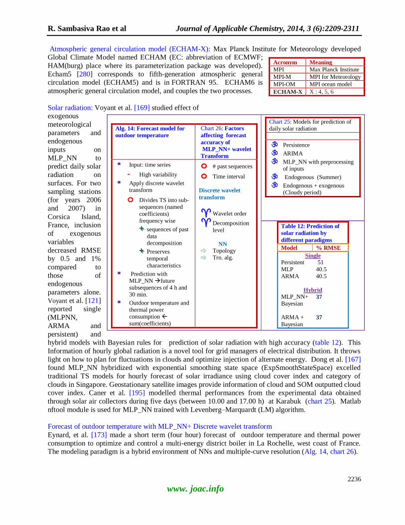
Atmospheric general circulation model (ECHAM-X): Max Planck Institute for Meteorology developed Global Climate Model named ECHAM (EC: abbreviation of ECMWF;
HAM(burg) place where its parameterization package was developed).
Echam5 [280] corresponds to fifth-generation atmospheric general circulation model (ECHAM5) and is in FORTRAN 95. ECHAM6 is
atmospheric general circulation model, and couples the two processes.
Solar radiation: Voyant et al. [169] studied effect of exogenous
meteorological
parameters and endogenous
inputs on
MLP_NN to predict daily solar
radiation on
surfaces. For two
sampling stations (for years 2006
and 2007) in
Corsica Island, France, inclusion
of exogenous
variables
decreased RMSE by 0.5 and 1%
compared to
those of endogenous
parameters alone.
Voyant et al. [121] reported single
(MLPNN,
ARMA and
persistent) and hybrid models with Bayesian rules for prediction of solar radiation with high accuracy (table 12). This
Information of hourly global radiation is a novel tool for grid managers of electrical distribution. It throws
light on how to plan for fluctuations in clouds and optimize injection of alternate energy. Dong et al. [167] found MLP_NN hybridized with exponential smoothing state space (ExpSmoothStateSpace) excelled
traditional TS models for hourly forecast of solar irradiance using cloud cover index and category of
clouds in Singapore. Geostationary satellite images provide information of cloud and SOM outputted cloud cover index. Caner et al. [195] modelled thermal performances from the experimental data obtained
through solar air collectors during five days (between 10.00 and 17.00 h) at Karabuk (chart 25). Matlab
nftool module is used for MLP_NN trained with Levenberg–Marquardt (LM) algorithm.
Forecast of outdoor temperature with MLP_NN+ Discrete wavelet transform
Eynard, et al. [173] made a short term (four hour) forecast of outdoor temperature and thermal power
consumption to optimize and control a multi-energy district boiler in La Rochelle, west coast of France. The modeling paradigm is a hybrid environment of NNs and multiple-curve resolution (Alg. 14, chart 26).
Acronym Meaning
MPI Max Planck Institute
MPI-M MPI for Meteorology
MPI-OM MPI ocean model
ECHAM-X X : 4, 5, 6
Alg. 14: Forecast model for
outdoor temperature
Chart 26: Factors
affecting forecast
accuracy of
MLP_NN+ wavelet
Transform
Input: time series
- High variability
Apply discrete wavelet transform
o Divides TS into sub-sequences (named
coefficients) frequency wise
sequences of past data decomposition
Preserves temporal
characteristics
Prediction with MLP_NN future subsequences of 4 h and 30 min.
Outdoor temperature and thermal power consumption sum(coefficients)
oo # past sequences
oo Time interval
Discrete wavelet
transform
Wavelet order
Decomposition
level
NN
Topology
Trn. alg.
Chart 25: Models for prediction of daily solar radiation
Persistence
ARIMA
MLP_NN with preprocessing of inputs
Endogenous (Summer)
Endogenous + exogenous (Cloudy period)
Table 12: Prediction of
solar radiation by
different paradigms
Model % RMSE
Single Persistent 51
MLP 40.5 ARMA 40.5
Hybrid MLP_NN+ Bayesian
37
ARMA +
Bayesian 37
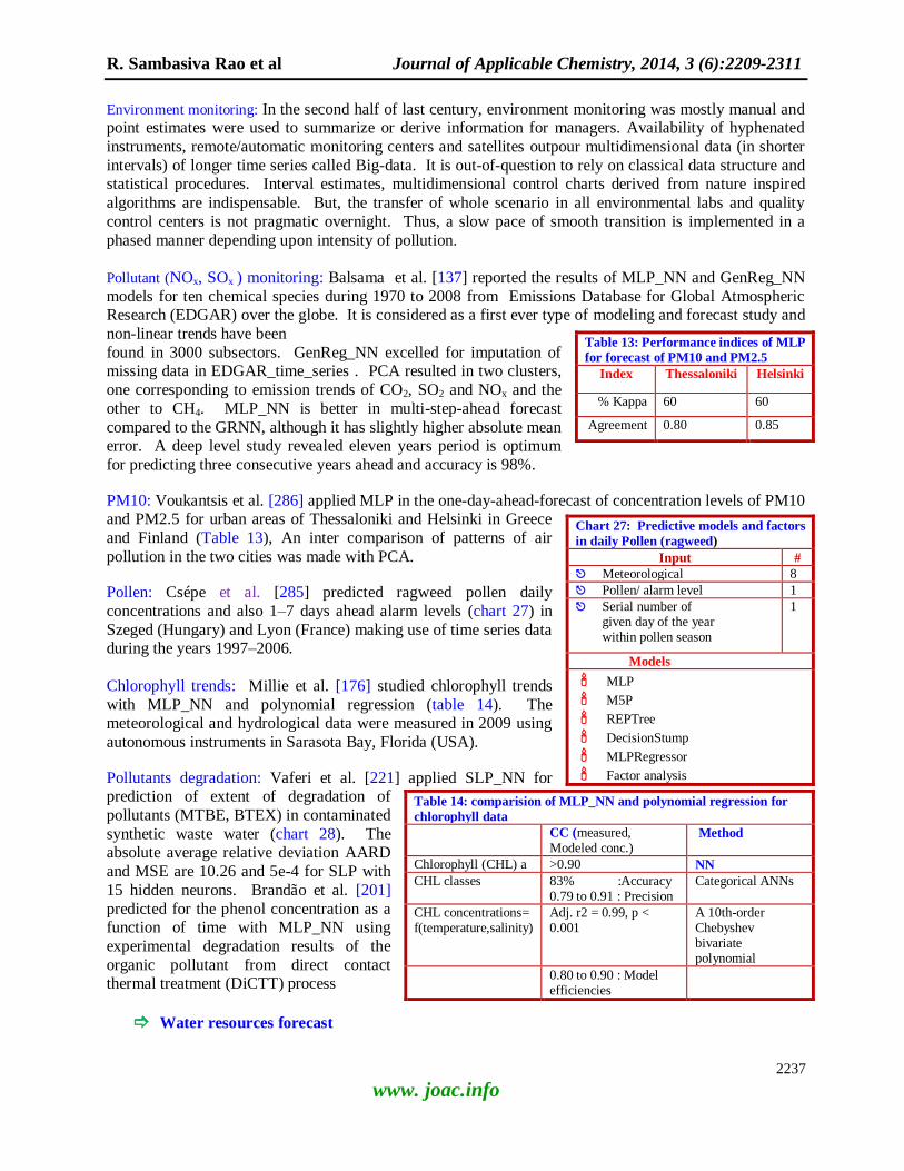
R. Sambasiva Rao et al Journal of Applicable Chemistry, 2014, 3 (6):2209-2311
2237
www. joac.info
Environment monitoring: In the second half of last century, environment monitoring was mostly manual and point estimates were used to summarize or derive information for managers. Availability of hyphenated
instruments, remote/automatic monitoring centers and satellites outpour multidimensional data (in shorter
intervals) of longer time series called Big-data. It is out-of-question to rely on classical data structure and statistical procedures. Interval estimates, multidimensional control charts derived from nature inspired
algorithms are indispensable. But, the transfer of whole scenario in all environmental labs and quality
control centers is not pragmatic overnight. Thus, a slow pace of smooth transition is implemented in a
phased manner depending upon intensity of pollution.
Pollutant (NOx, SOx ) monitoring: Balsama et al. [137] reported the results of MLP_NN and GenReg_NN
models for ten chemical species during 1970 to 2008 from Emissions Database for Global Atmospheric Research (EDGAR) over the globe. It is considered as a first ever type of modeling and forecast study and
non-linear trends have been
found in 3000 subsectors. GenReg_NN excelled for imputation of missing data in EDGAR_time_series . PCA resulted in two clusters,
one corresponding to emission trends of CO2, SO2 and NOx and the
other to CH4. MLP_NN is better in multi-step-ahead forecast
compared to the GRNN, although it has slightly higher absolute mean error. A deep level study revealed eleven years period is optimum
for predicting three consecutive years ahead and accuracy is 98%.
PM10: Voukantsis et al. [286] applied MLP in the one-day-ahead-forecast of concentration levels of PM10 and PM2.5 for urban areas of Thessaloniki and Helsinki in Greece
and Finland (Table 13), An inter comparison of patterns of air
pollution in the two cities was made with PCA.
Pollen: Csépe et al. [285] predicted ragweed pollen daily
concentrations and also 1–7 days ahead alarm levels (chart 27) in
Szeged (Hungary) and Lyon (France) making use of time series data during the years 1997–2006.
Chlorophyll trends: Millie et al. [176] studied chlorophyll trends
with MLP_NN and polynomial regression (table 14). The meteorological and hydrological data were measured in 2009 using
autonomous instruments in Sarasota Bay, Florida (USA).
Pollutants degradation: Vaferi et al. [221] applied SLP_NN for prediction of extent of degradation of
pollutants (MTBE, BTEX) in contaminated
synthetic waste water (chart 28). The absolute average relative deviation AARD
and MSE are 10.26 and 5e-4 for SLP with
15 hidden neurons. Brandão et al. [201]
predicted for the phenol concentration as a function of time with MLP_NN using
experimental degradation results of the
organic pollutant from direct contact thermal treatment (DiCTT) process
Water resources forecast
Table 13: Performance indices of MLP
for forecast of PM10 and PM2.5
Index Thessaloniki Helsinki
% Kappa 60 60
Agreement 0.80 0.85
Chart 27: Predictive models and factors
in daily Pollen (ragweed)
Input #
Meteorological 8
Pollen/ alarm level 1
Serial number of given day of the year within pollen season
1
Models
MLP
M5P
REPTree
DecisionStump
MLPRegressor
Factor analysis
Table 14: comparision of MLP_NN and polynomial regression for
chlorophyll data
CC (measured, Modeled conc.)
Method
Chlorophyll (CHL) a >0.90 NN
CHL classes 83% :Accuracy 0.79 to 0.91 : Precision
Categorical ANNs
CHL concentrations= f(temperature,salinity)
Adj. r2 = 0.99, p < 0.001
A 10th-order Chebyshev bivariate polynomial
0.80 to 0.90 : Model efficiencies
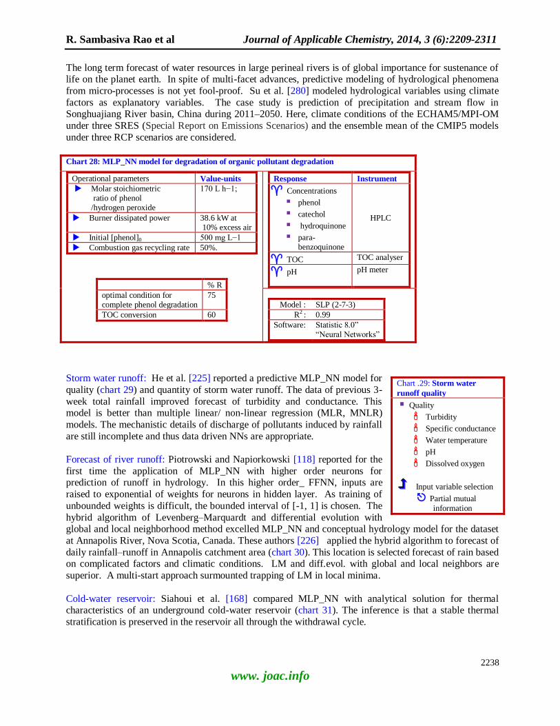
R. Sambasiva Rao et al Journal of Applicable Chemistry, 2014, 3 (6):2209-2311
2238
www. joac.info
The long term forecast of water resources in large perineal rivers is of global importance for sustenance of life on the planet earth. In spite of multi-facet advances, predictive modeling of hydrological phenomena
from micro-processes is not yet fool-proof. Su et al. [280] modeled hydrological variables using climate
factors as explanatory variables. The case study is prediction of precipitation and stream flow in Songhuajiang River basin, China during 2011–2050. Here, climate conditions of the ECHAM5/MPI-OM
under three SRES (Special Report on Emissions Scenarios) and the ensemble mean of the CMIP5 models
under three RCP scenarios are considered.
Chart 28: MLP_NN model for degradation of organic pollutant degradation
Operational parameters Value-units
Molar stoichiometric ratio of phenol /hydrogen peroxide
170 L h−1;
Burner dissipated power
38.6 kW at 10% excess air
Initial [phenol]0 500 mg L−1
Combustion gas recycling rate 50%.
% R
optimal condition for complete phenol degradation
75
TOC conversion 60
Response Instrument
Concentrations
phenol
catechol
hydroquinone
para-benzoquinone
HPLC
TOC TOC analyser
pH
pH meter
Model : SLP (2-7-3)
R2 : 0.99
Software: Statistic 8.0‖ ―Neural Networks‖
Storm water runoff: He et al. [225] reported a predictive MLP_NN model for
quality (chart 29) and quantity of storm water runoff. The data of previous 3-
week total rainfall improved forecast of turbidity and conductance. This model is better than multiple linear/ non-linear regression (MLR, MNLR)
models. The mechanistic details of discharge of pollutants induced by rainfall
are still incomplete and thus data driven NNs are appropriate.
Forecast of river runoff: Piotrowski and Napiorkowski [118] reported for the
first time the application of MLP_NN with higher order neurons for prediction of runoff in hydrology. In this higher order_ FFNN, inputs are
raised to exponential of weights for neurons in hidden layer. As training of
unbounded weights is difficult, the bounded interval of [-1, 1] is chosen. The
hybrid algorithm of Levenberg–Marquardt and differential evolution with global and local neighborhood method excelled MLP_NN and conceptual hydrology model for the dataset
at Annapolis River, Nova Scotia, Canada. These authors [226] applied the hybrid algorithm to forecast of
daily rainfall–runoff in Annapolis catchment area (chart 30). This location is selected forecast of rain based on complicated factors and climatic conditions. LM and diff.evol. with global and local neighbors are
superior. A multi-start approach surmounted trapping of LM in local minima.
Cold-water reservoir: Siahoui et al. [168] compared MLP_NN with analytical solution for thermal characteristics of an underground cold-water reservoir (chart 31). The inference is that a stable thermal
stratification is preserved in the reservoir all through the withdrawal cycle.
Chart .29: Storm water
runoff quality
Quality
Turbidity
Specific conductance
Water temperature
pH
Dissolved oxygen
Input variable selection
Partial mutual
information

R. Sambasiva Rao et al Journal of Applicable Chemistry, 2014, 3 (6):2209-2311
2239
www. joac.info
Prediction of water resources
Rampone [128] applied MLP_NN to predict 3- and 6- months ahead of water resources at karstic aquifers in the Terminio massif (Southern Italy), especially in high stress months of July and August. The rainfall–
discharge relationships are modeled with tenfold CV for the aquifer which supplies water in the Naples
area, Southern Italy. The three-month and six-month-ahead discharge forecast errors are 5 and 10%.
Evapotranspiration: Cobaner [227] compared the performance of grid partition and subtractive clustering
based ANFIS and MLP NNs for evapotranspiration (ET0) data in Los Angeles. FAO-56 Penman–
Monteith equation is used to calculate ET0. A comparative study showed S-ANFIS excels MLP (chart 32) and CIMIS Penman, Hargreaves_Ritchie methods based on RMSE, R
2 and MAD.
Waste water treatment: Bagheri et al. [278] applied MLP_NN and RBF_NN to model data of municipal
wastewater treatment (chart 33) in a sequential batch reactor.
Wastewater treatment plant: Ay and Kisi [228] integrated MLP with k-means and applied in modeling of
COD in the upstream of the municipal wastewater treatment plant at Adapazari province of Turkey. The
Chart 30: Complex factors in runoff and training
algorithms for MLP_NN
Levenberg–Marquardt Alg.
Versus
River flow
characteristics
Differential Evolution (Diff.Evol.) (version 1)
Distributed Diff.Evol. with Explorative–Exploitative Population Self-Adaptive DE
Diff.Evol. with global and local neighbors
Grouping Diff.Evol.
JADE
PSO
Comprehensive learning
Efficient population utilization strategy PSO
Seasonal changes in
runoff Rapid floods Dry summers Severe winters
with snowfall Snow melting Frequent freeze
and thaw
Presence of river ice
Chart 32: Input for evapotranspiration model Input
Sodium chloride
Concentration in feed solution, C
Feed temperature, T
Feed flow-rate, Q
Operating hydrostatic pressure, P Response RO performance index
Optimum operating conditions
Four input variables
Brackish water 6 g/L
30 g/L
Chart 31: Underground cold-water reservoir thermal stratification
Boundary condition of temperature distribution in reservoir
Linearized Analytical soln
Non-linear MLP_NN
Chart 32b: Comparative modeling of evapotranspiration
Input (daily climaticdata)
Solar radiation,
Air temperature,
Relative humidity
Wind speed
Sampling site
Santa Monica, LA, USA
Models
NN
MLP
Empirical
CIMIS Penman, Hargreaves Ritchie
Perforance statistics Root mean square error Mean absolute error Determination coefficient
Inference: S-ANFIS >> [G-ANFIS and MLP]
G-: Grid
S-: Subtractive clustering

R. Sambasiva Rao et al Journal of Applicable Chemistry, 2014, 3 (6):2209-2311
2240
www. joac.info
input variables are daily measured pH, discharge, temperature and TDS. The hybridization of MLP_NN and k-means is superior in terms of RMS, mean absolute error and R in prediction. The results of MLR,
MLP_NN, RBF_NN, subtractive clustering /grid-
partition FIS_NN models are compared.
Automatic detection of bin level and amount of solid
waste: Earlier, many approaches viz. GIS,
Radio-frequency Identification (RFID), or sensor intelligent bins have been proposed for Solid Waste
Management (SWM) system. The key point is to fix
the position of camera to obtain bin image. Islam, et
al. [300] put forward dynamic time warping (DTW) procedure to detect and crop the bin area. The features
of image of bin are calculated with Gabor wavelet
(GW) and inputted to MLP_NN. The output consists of level of bin and amount of waste inside it. The
statistical analysis of classification is performed with
ROC and the achieved accuracy in this study is
98.50%. Hannan et al. [301] proposed MLP_NN to detect automatically the waste bin level of filling ((table 15).). The bin image texture is analyzed with gray
level aura matrix (GLAM) approach.
Crack propagation in pavement ([MLP or RBF] + FiniteEleMeth): Gajewski et al. [150] made sensitivity analysis of non- destructive testing of crack
propagation in pavement bituminous
layered structures with hybridization of FF_NNs (MLP, RBF) with finite element method (chart 34). The outcome is cracking increases with lowering
the bituminous layer (B2) thickness. The cracking of the subgrade layer is
less influenced by asphalt layer (B1) thickness.
Desalination: Khayet et al. [233] compared predictive models for desalination by reverse osmosis (RO) process with RSM and NN models. NN far excelled the sought after
quadratic RSM model.
The maximum RO performance indexes are experimentally attained with optimum operating conditions from Monte Carlo simulations.
Ocean floor: Kajiyama et al. [276] predicted execution time of MC
simulations with MLP_NN. The input data are execution times recorded for different cases of simulation under a variety of environments. The
ultimate goal this pursuit is prediction of execution times for simulations of parallel Monte Carlo (MC)
radiative transfer with applications in ocean color.
Geometrics (Geology + metrics)
MLP_NN + PSO for rock fractal parameters: The determination of fractal dimension of roughness profiles (D) is still a complicated task due to both stochastic and systematic errors which cannot be
Chart 33: Wastewater treatment with MLP_NN
and RBF_NN
Input Output
Influent concentration (IC) Filling time (FT)
Reaction time (RT) Aeration intensity (AI)
SRT MLVSS concentration
Effluent concentrations TSS
TP COD
NH4+-N
Optimum conditions
FT 1 h
RT 6 h
Aeration intensity
0.88 m3/min
SRT 30 days
Removal efficiencies
TSS 86
TP 79
COD 94
NH4+-
nitrogen
93
Inference : MLP_NN > RBF_NN
Table 15: solid waste bin
level detection with gray level
aura matrix
Model %Classification
Class Grade
MLP 98.98 90.19
k-NN 96.91 89.14
Chart 34: Input to [MLP or
RBF] + FiniteEleMeth
Inputs For each layer of creating pavement
Thickness of layers
Load value
Young‘s moduli end
Alg. 15: Hybrid MLP_NN and PSO
for fractal parameters of rocks
Step 0 Simulate large number of fractional
Brownian profiles at varying numerical
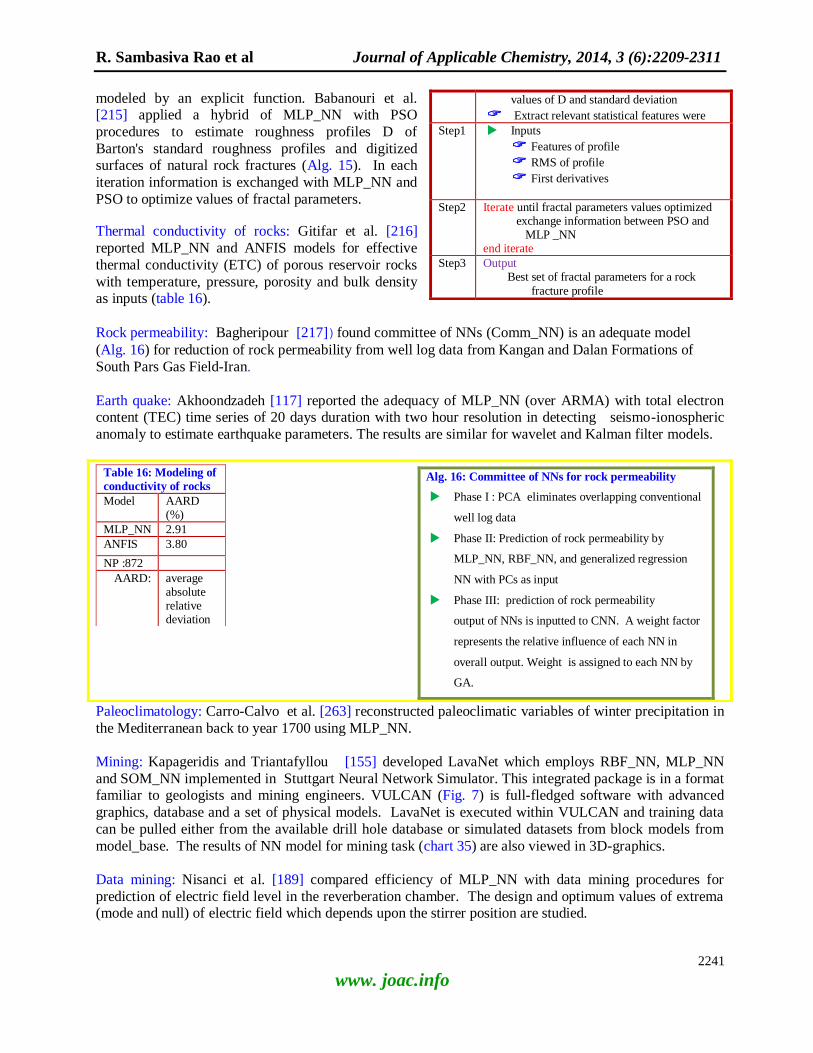
R. Sambasiva Rao et al Journal of Applicable Chemistry, 2014, 3 (6):2209-2311
2241
www. joac.info
modeled by an explicit function. Babanouri et al. [215] applied a hybrid of MLP_NN with PSO
procedures to estimate roughness profiles D of
Barton's standard roughness profiles and digitized surfaces of natural rock fractures (Alg. 15). In each
iteration information is exchanged with MLP_NN and
PSO to optimize values of fractal parameters.
Thermal conductivity of rocks: Gitifar et al. [216]
reported MLP_NN and ANFIS models for effective
thermal conductivity (ETC) of porous reservoir rocks
with temperature, pressure, porosity and bulk density as inputs (table 16).
Rock permeability: Bagheripour [217])found committee of NNs (Comm_NN) is an adequate model
(Alg. 16) for reduction of rock permeability from well log data from Kangan and Dalan Formations of
South Pars Gas Field-Iran.
Earth quake: Akhoondzadeh [117] reported the adequacy of MLP_NN (over ARMA) with total electron content (TEC) time series of 20 days duration with two hour resolution in detecting seismo-ionospheric
anomaly to estimate earthquake parameters. The results are similar for wavelet and Kalman filter models.
Paleoclimatology: Carro-Calvo et al. [263] reconstructed paleoclimatic variables of winter precipitation in
the Mediterranean back to year 1700 using MLP_NN.
Mining: Kapageridis and Triantafyllou [155] developed LavaNet which employs RBF_NN, MLP_NN
and SOM_NN implemented in Stuttgart Neural Network Simulator. This integrated package is in a format familiar to geologists and mining engineers. VULCAN (Fig. 7) is full-fledged software with advanced
graphics, database and a set of physical models. LavaNet is executed within VULCAN and training data
can be pulled either from the available drill hole database or simulated datasets from block models from
model_base. The results of NN model for mining task (chart 35) are also viewed in 3D-graphics.
Data mining: Nisanci et al. [189] compared efficiency of MLP_NN with data mining procedures for
prediction of electric field level in the reverberation chamber. The design and optimum values of extrema (mode and null) of electric field which depends upon the stirrer position are studied.
values of D and standard deviation
Extract relevant statistical features were
Step1 Inputs
Features of profile
RMS of profile
First derivatives
Step2 Iterate until fractal parameters values optimized exchange information between PSO and MLP _NN end iterate
Step3 Output Best set of fractal parameters for a rock
fracture profile
Table 16: Modeling of
conductivity of rocks
Model AARD (%)
MLP_NN 2.91
ANFIS 3.80
NP :872
AARD: average absolute relative deviation
Alg. 16: Committee of NNs for rock permeability
Phase I : PCA eliminates overlapping conventional
well log data
Phase II: Prediction of rock permeability by
MLP_NN, RBF_NN, and generalized regression
NN with PCs as input
Phase III: prediction of rock permeability
output of NNs is inputted to CNN. A weight factor
represents the relative influence of each NN in
overall output. Weight is assigned to each NN by
GA.
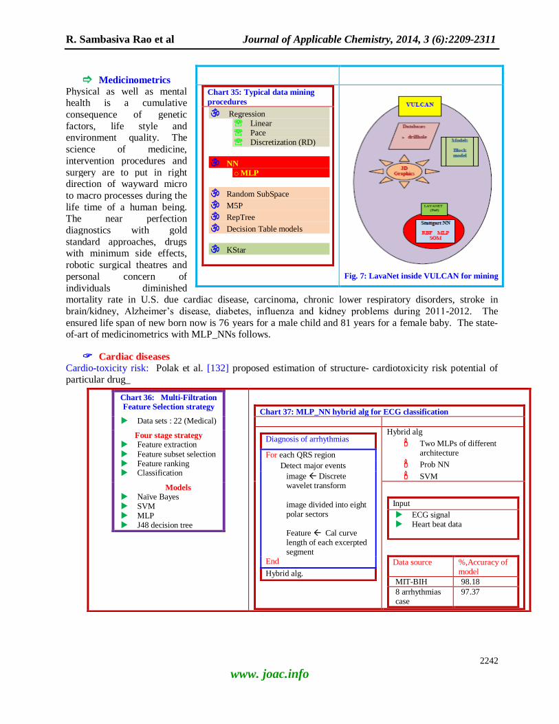
R. Sambasiva Rao et al Journal of Applicable Chemistry, 2014, 3 (6):2209-2311
2242
www. joac.info
Medicinometrics
Physical as well as mental health is a cumulative
consequence of genetic
factors, life style and environment quality. The
science of medicine,
intervention procedures and
surgery are to put in right direction of wayward micro
to macro processes during the
life time of a human being. The near perfection
diagnostics with gold
standard approaches, drugs with minimum side effects,
robotic surgical theatres and
personal concern of
individuals diminished mortality rate in U.S. due cardiac disease, carcinoma, chronic lower respiratory disorders, stroke in
brain/kidney, Alzheimer‘s disease, diabetes, influenza and kidney problems during 2011-2012. The
ensured life span of new born now is 76 years for a male child and 81 years for a female baby. The state-of-art of medicinometrics with MLP_NNs follows.
Cardiac diseases
Cardio-toxicity risk: Polak et al. [132] proposed estimation of structure- cardiotoxicity risk potential of particular drug_
Chart 35: Typical data mining
procedures
Regression Linear Pace Discretization (RD)
NN
o MLP
Random SubSpace
M5P
RepTree
Decision Table models
KStar
Fig. 7: LavaNet inside VULCAN for mining
Chart 36: Multi-Filtration Feature Selection strategy
Data sets : 22 (Medical)
Four stage strategy Feature extraction
Feature subset selection Feature ranking Classification
Models Naïve Bayes SVM MLP J48 decision tree
Chart 37: MLP_NN hybrid alg for ECG classification
Diagnosis of arrhythmias
For each QRS region
Detect major events
image Discrete wavelet transform
image divided into eight polar sectors Feature Cal curve length of each excerpted segment
End
Hybrid alg.
Hybrid alg
Two MLPs of different architecture
Prob NN
SVM
Input
ECG signal Heart beat data
Data source %,Accuracy of model
MIT-BIH 98.18
8 arrhythmias case
97.37
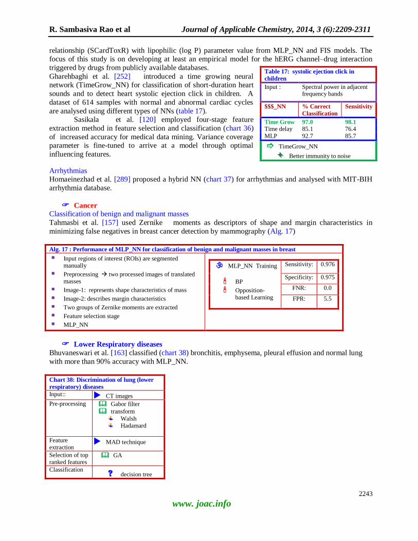
R. Sambasiva Rao et al Journal of Applicable Chemistry, 2014, 3 (6):2209-2311
2243
www. joac.info
relationship (SCardToxR) with lipophilic (log P) parameter value from MLP_NN and FIS models. The focus of this study is on developing at least an empirical model for the hERG channel–drug interaction
triggered by drugs from publicly available databases.
Gharehbaghi et al. [252] introduced a time growing neural network (TimeGrow_NN) for classification of short-duration heart
sounds and to detect heart systolic ejection click in children. A
dataset of 614 samples with normal and abnormal cardiac cycles
are analysed using different types of NNs (table 17). Sasikala et al. [120] employed four-stage feature
extraction method in feature selection and classification (chart 36)
of increased accuracy for medical data mining. Variance coverage parameter is fine-tuned to arrive at a model through optimal
influencing features.
Arrhythmias Homaeinezhad et al. [289] proposed a hybrid NN (chart 37) for arrhythmias and analysed with MIT-BIH
arrhythmia database.
Cancer Classification of benign and malignant masses
Tahmasbi et al. [157] used Zernike moments as descriptors of shape and margin characteristics in
minimizing false negatives in breast cancer detection by mammography (Alg. 17)
Alg. 17 : Performance of MLP_NN for classification of benign and malignant masses in breast
Input regions of interest (ROIs) are segmented manually
Preprocessing two processed images of translated masses
Image-1: represents shape characteristics of mass
Image-2: describes margin characteristics
Two groups of Zernike moments are extracted
Feature selection stage
MLP_NN
MLP_NN Training
BP
Opposition-based Learning
Sensitivity: 0.976
Specificity: 0.975
FNR: 0.0
FPR: 5.5
Lower Respiratory diseases
Bhuvaneswari et al. [163] classified (chart 38) bronchitis, emphysema, pleural effusion and normal lung
with more than 90% accuracy with MLP_NN.
Chart 38: Discrimination of lung (lower
respiratory) diseases
Input:: CT images
Pre-processing Gabor filter
transform
Walsh Hadamard
Feature extraction
MAD technique
Selection of top ranked features
GA
Classification ? decision tree
Table 17: systolic ejection click in
children
Input : Spectral power in adjacent frequency bands
$$$_NN % Correct
Classification
Sensitivity
Time Grow 97.0 98.1 Time delay 85.1 76.4 MLP 92.7 85.7
TimeGrow_NN
Better immunity to noise

R. Sambasiva Rao et al Journal of Applicable Chemistry, 2014, 3 (6):2209-2311
2244
www. joac.info
? KNN
? MLP-NN
CT: Computed tomography
MAD: Mean absolute deviation
Liver transplantation
Child–Pugh–Turcotte score: The subjective and objective clinical parameters (chart 39) determine the
score and are used for liver
transplantation (LT) based on ‗sicker patient first‘. Here
subjective parameters are
influenced by treatment with diuretics or paracentesns for
ascites and lactulose for
encephalopathy. Mayo model was later named as MELD and
predicts three months mortality of
227 in queue for LT (chart 40).
This is taken as priority level to overcome normal waiting pattern
‗sicker patient first‘. It was found
MLP_NN with 18 different liver transplant recipient and donor
variables predicted more
accurately outcomes post-LT compared to MELD and SOFA
scores. Singal et al. [219]
reviewed the state-of-the-art-MLED and opines that it continues to be an acceptable score till a new one
comes into prominence with authority and approval.
Brain and CNS disorders
Resting state network (RSN) from fMRI: Hacker et al. [267] modeled blood oxygen level dependent
(BOLD) correlation maps with specific resting state network (RSN) identities with MLP_NN. The
network outputs more spatially specific RSN maps compared to dual regression and LDA. Further, RSN
topography values in individuals are correct even in the brain regions not represented in the training dataset.
Detection of Alzheimer's disease: Park et al. [148] detected Alzheimer's disease with 95.8% classification accuracy from analysis of 272 Raman spectra of platelets in rat blood with MLP_NN (chart 41). The
features chosen are intensity at 1658 cm− 1 and ratio of intensity of 757 to that at 743 cm− 1
correponding
to amide I mode and cytochrome c.
EEG
Basic emotions and facial expression: The facial/verbal expressions of a human being for a visual/ psychological stimulus (chart 42) are common across the cultures. In fact, they are selected by nature and
are due to their high survival factors. Rahnuma et al. [273] classified EEG signals corresponding to four
emotions (happy, calm, sad and fear) with MLP_NN using inputs of features obtained from kernel density
Chart 39: Liver
allocation score Objective
Severity 1. Serum albumin 2. Serum bilirubin
3. Prothrombin time
Subjective
4. Ascites 5. Encephalopathy
Liver disease
CTP Child–Pugh–Turcotte
HRS Hepatorenal syndrome
LT Liver transplantation
MELD Model for end-stage liver disease
SOFA Sequential organ failure assessment
Chart 40: MELD score
Best predictor of Survival period after transjugular intrahepatic portosystemic shunt Mortality of patents with end-stage liver disease
Survival of patients with alcoholic hepatitis, following variceal hemorrhage, infections in cirrhosis
Post-surgical life span of patients with cirrhosis including liver resection, trauma, and hepato-renal syndrome

R. Sambasiva Rao et al Journal of Applicable Chemistry, 2014, 3 (6):2209-2311
2245
www. joac.info
estimation. EEG of eight healthy subjects from different states in Malasia is recorded and the study is with an objective of probing into effects of depression and stress on mental health. Shams et al. [272] proposed
emotion recognition system (Emot.Recog.) from Electroencephalographic (EEG) signals. The subjects of
this study are ten healthy kids of 5 to 6 years and are shown photographs from Radbound faces database (RaFD) followed by EEG analysis for basic emotions (Chart 43). Majumder et al. [269] used extended
Kohonen_SOM for recognition of six basic emotions in facial expression with data from MMI facial
expression database. The analytical face model with 26 features is integrated within the algorithm. The
comparison of results show superiority of SOM_NN over MLP_NN, RBF_NN etc. (chart 44). Danisman et
al. [291] used MLP in recognition of facial expression. The best and worst feature window position for a set
of face images from GENKI, JAFFE and FERET databases are obtained from exhaustive searches. It
leads to a non-rectangular emotion mask and eliminates irrelevant data. The backward elimination of features further enhances the performance.
Chart 41: Raman spectra for
Alzheimer's detection 278 Raman spectra
Preprocessing
Separate all significants peaks
Find most discriminat peak as a reference feature
Cal cc(most significant peak vs all peaks)
Discard highly correlated peaks
Preliminary classification
Peak value and their ratio of the remaining features
10% cases with most frequently appearing features are picked up
Classification
Chart 44: Facial expression Database
MMI facial expression database
Analytical face model
Eye, lip and eyebrow
feature points
26-Dimensional geometric feature vector
MLP_NN
RBF_NN
Kohonen_SOM Ext.SOM > [mcSVM, MLP, RBF]
Chart 42: Emotions of humans
Basic emotions
Neutral Happy
Sad
Fear Anger
Surprise
Disgust
Complex (Combination of basic) emotions
Shame
Disappointment
Chart 43: Analysis of emotions
in kids with EEG
Feature extraction Time Difference of Arrival
Classification Regul.LS
MLP
Wavelet coefficients
% Correct Classification
User independent 96
User dependent 100
Dermatology Özçift et al. [161] compared MLP, Bayesian network wrapped with GA to diagnose six dermatological
diseases. The most influential features out of 34 in the erythemato-squamous dataset are selected by GA in
the hybrid approach and the accuracy of classification is 99.2% (Table 18). GA was found to be far superior to sequential floating methods.
(Human) Skin color classification
Detection and quantitative measure of skin color is vital in tracking of human body parts, face/ naked
people detection/ recognition, retrieval of a person in multimedia databases and human computer interaction. Razmjooy et al. [249] proposed hybrid MLP_NN and Imperialist competitive algorithm

R. Sambasiva Rao et al Journal of Applicable Chemistry, 2014, 3 (6):2209-2311
2246
www. joac.info
(Imp.Compet.Alg) in solving human skin color classification. The socio-political processes of imperialistic competition of mankind in the real world are the inspiration and it makes searches for
high quality solutions with minimum classification error, while MLP_NN take care of constraints of task.
Clinical analysis (Chemometrics + soft_sensors + Clinical procedures)
Sharma and Tambe [139] compared efficiency of soft sensor (SS) based
MLP_NN, SVR, genetic programming (GP) to predict time-dependent
lipase activity and amount of accumulated polyhydroxyalkanoates. Soft-sensors are software based process monitoring systems which searches and
optimizes both the form (structure) and parameters of NNs. GP_SS are
superior to MLP_NN based on RMS and R (Table 19).
Diagnosis of Collagenous Colitis: Malekian et al. [253] reported screening of
Collagenous Colitis (CC) with MLP_NN using colon tissue images. Chronic watery diarrhea is a symptom of microscopic colitis, but
endoscopic and radiographic tests show normal. The gold standard for a
confirmative diagnosis of CC is measurement of thickness of the sub-
epithelial collagen (SEC) from colon tissue biopsy samples.
Biochemical studies (Biometrics + Chemometrics + soft sensors)
Microarray technology -- DNA-Genes: DNA is one of the most complicated codes in nature and its
tracking is now a sought after venture. Thousands of spots in a micro-array image correspond to different
genes. The segmentation of image is to match gene with pixels. The noise and variation of pixels makes
the task harder. Wang et al. [151] found MLP_NN and Kohonen_NN resulted in superior peak signal-to-noise ratio (PSNR) for cDNA images compared to GenePix®.
Electric (power) engineering Transient stability assessment: Sharifian and Sharifian [210] reported hybridization of MLP_NN with
type-2_fuzzy_NN for transient stability assessment (TSA) in power systems (chart 45). For every
disturbance causing a fault in TSA, many non-linear equations need to be solved requiringhigh cpu time. It leads to delayed actions for signal control rendering the situation alarming. With the hybrid data-driven AI
approach, the accurate estimation of critical clearing time, an index of TSA is done and the system is
scaled up to a large power system.
Household consumption: Azadeh and Faiz [134] made a critical study of annual household electricity
consumption (chart 46) in Iran during the period 1974 to 2003 and found MLP_NN along with
experimental design has superior performance.
Robots Inverse kinematics: Aggarwal et al. [274] reported an inverse kinematic solution for a PUMA 560 robot
with MLP_NN trained with robot's end-effector Cartesian co-ordinates along with corresponding
configurations at joints. The trained NN predicts the behavior more confidently
Table 18: Comparison of
Methods for dermatological
diseases
Method %Accuracy
SVM 98.36
MLP 97.00
Simple Logistics
98.36
Functional Decision Tree
97.81
GA wrapped +
Bayesian Network
Accuracy % 99.20
Misclassification
number
3 out of 366
Table 19: Comparison of efficiency of soft sensor based models
Process Prediction Soft sensor based on
GP SVR MLP_NN
Extracellular production of lipase enzyme Time-dependent lipase activity (U/ml) 0.96 <<0.96 <<0.96
Bacterial production of poly(3-hydroxybutyrate-co-3-hydroxyvalerate) copolymer
Amount of accumulated polyhydroxyalkanoates (% dcw)
0.98 0.98 0.94
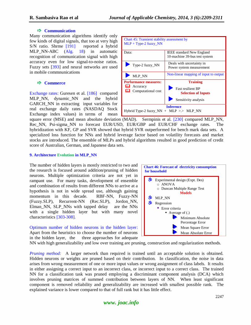
R. Sambasiva Rao et al Journal of Applicable Chemistry, 2014, 3 (6):2209-2311
2247
www. joac.info
Communication
Many communication algorithms identify only
few kinds of digital signals, that too at very high S/N ratio. Shrme [191] reported a hybrid
MLP_NN-ABC (Alg. 18) in automatic
recognition of communication signal with high accuracy even for low signal-to-noise ratios.
Fuzzy sets [393] and neural networks are used
in mobile commnunications
Commerce
Exchange rates: Guresen et al. [186] compared
MLP_NN, dynamic_NN and the hybrid
GARCH_NN in extracting input variables for real exchange daily rates (NASDAQ Stock
Exchange index values) in terms of mean
square error (MSE) and mean absolute deviation (MAD). Sermpinis et al. [230] compared MLP_NN, Rec_NN, Psi-sigma_NN to forecast EUR/USD, EUR/GBP and EUR/CHF exchange rates. The
hybridization with KF, GP and SVR showed that hybrid SVR outperformed for bench mark data sets. A
specialized loss function for NNs and hybrid leverage factor based on volatility forecasts and market
stocks are introduced. The ensemble of MLPs and hybrid algorithms resulted in good prediction of credit score of Australian, German, and Japanese data sets.
9. Architecture Evolution in MLP_NN
The number of hidden layers is mostly restricted to two and the research is focused around addition/pruning of hidden
neurons. Multiple optimization criteria are not yet in
rampant use. For many tasks, development of ensemble and combination of results from different NNs to arrive at a
hypothesis is not in wide spread use, although gaining
momentum in this decade. RBF-NN, Fuzzy-NN (Fuzzy.SLP), Recurrent-NN (Rec.SLP), Jordon_NN,
Elman_NN, SLP_NNs with tapped delay are the NNs
with a single hidden layer but with many novel
characteristics [303-308].
Optimum number of hidden neurons in the hidden layer:
Apart from the heuristics to choose the number of neurons in the hidden layer, the three approaches for adequate
NN with high generalizability and low over training are pruning, construction and regularization methods.
Pruning method: A larger network than required is trained until an acceptable solution is obtained. Hidden neurons or weights are pruned based on their contribution. In classification, the noise in data
arises from wrong measurement of one or more input values or wrong assignment of class labels. It results
in either assigning a correct input to an incorrect class, or incorrect input to a correct class. The trained NN for a classification task was pruned employing a discriminant component analysis (DCA) which
involves pruning matrices of summed contribution between layers of NN. When least significant
component is removed reliability and generalizability are increased with smallest possible rank. The explained variance is lower compared to that of full rank but it has little effect.
Chart 45: Transient stability assessment by MLP + Type-2 fuzzy_NN
Data: IEEE standard New England 10-machine 39-bus test system
Type-2 fuzzy_NN Deals with uncertainty in Power system measurement
MLP_NN Non-linear mapping of input to output
Performance measures:
Accuracy
Computational cost
Training
Fast resilient BP
Selection of Inputs
Sensitivity analysis
Inference Hybrid Type-2 fuzzy_NN + MLP >.> MLP_NN
Chart 46: Forecast of electricity consumption
for household
Experimental design (Expt. Des) o ANOVA o Duncan Multiple Range Test
Models
MLP_NN
Regression
Error criteria Average of (.)
Minimum Absolute
Percentage Error
Mean Square Error
Mean Absolute Error

R. Sambasiva Rao et al Journal of Applicable Chemistry, 2014, 3 (6):2209-2311
2248
www. joac.info
Constructive method: A NN of minimum architecture
(I#-1-O#) i.e. with a single hidden neuron is trained.
Then the neurons are added followed by layers until an adequate model is arrived or convergence criteria are
met.
Combination of methods: Recently constructive and pruning algorithms are implemented together to
automatic selection of FF-NN architecture. An
interesting attempt is in combining pruning, optimal brain surgeon algorithm, quadratic regression
(Quad.Reg.) in subset based training.
MLP with splitting H1 layer into sub units: The hidden
layer of the assembly NN is split into sub-units equal to
the number of output classes. Further, the sub-units are interconnected in a feed forward manner in
addition to direct connections [73].
Centroid based MLP_NN (MLP.centroid.)
Lehatokangas [15] proposed centroid based MLP_NN with two hidden layers (HLs). Here, in the first
hidden (called centroid) layer, inverse principal component analysis (inverse_PCA) is performed. Adaptive centroid vectors, which correspond to kernel centers, are used and the output of each centroid unit becomes
the Euclidean distance between input and centroid vectors. Here, a special transformation of input data is
performed which is akin to radial basis layer of RBF. A sigmoid TF is used in the second HL. Then number of centroids, their co-ordinates and weight vectors (WH1H2 and WH2O) are refined with BP. The
advantage is PCA of X-matrix reduces the number of centroids to a remarkable level. The first step of
algorithm calculates approximate lower bound used as starting point by PCA. In the next phase, the
adequate minimum number of centroids is estimated at a user specified level of accuracy. It results in a compact (less complicated) architecture even for difficult classification tasks. The number of centroid units
was determined empirically.
Dynamic architecture-2 (DA2-)-MLP_NN
The closed form of set equations are solved [6], partially alleviating black box dilemma of NNs. The
number of neurons is fixed to four. The initial
architecture consists of a single layer with connections I --> G1 --> F1, I --> F0 --> F1, I --> H1 --> F1 and
bias to F1. Sine, cosine and linear transfer functions
are used in G1, H1 and F0 respectively. The number of layers is limited by the desired accuracy. The linear
component is calculated in the neuron F0 and sine and
cosine of input are estimated with H and G neurons.
F1 collects the weighted outputs of F0, G1 and H1. If the residual is greater than the convergence limit, an
additional layer is added and the process is repeated.
At each stage the four neurons viz. G, H, F and bias constituting a new layer is added and the five
parameters are calculated.
In this NN, The parameters are estimated with both
non-gradient (bisection, golden search, Brent) and first order gradient (DSC-Powell, Fletcher-Reeves) non-
Alg. 18: MLP_NN +ABC in
communications
Tr.Alg :
Quick prop (QP)
Extended delta-bar-delta (EDBD)
Super self adaptive back
propagation (supersab)
Conjugate gradient (CG)]
Input : Communication signal
Phase I
Cal higher (up to eighth)
order moments
Features cumulants of higher (up to eighth) order moments
MLP_NN as a classifier
Phase II
Selection of the best features with Bees Algorithm (BA)
Output: Discriminated signals
Entire data set is analyzed in one stroke instead of presenting pattern by pattern
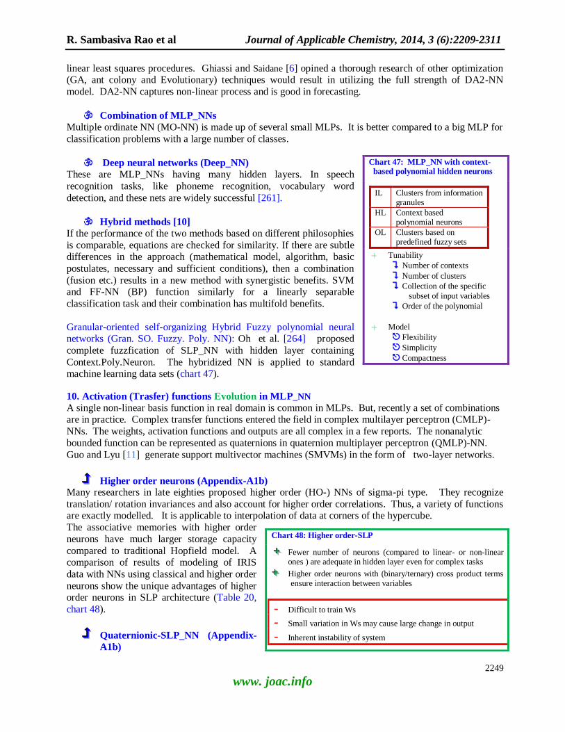
R. Sambasiva Rao et al Journal of Applicable Chemistry, 2014, 3 (6):2209-2311
2249
www. joac.info
linear least squares procedures. Ghiassi and Saidane [6] opined a thorough research of other optimization (GA, ant colony and Evolutionary) techniques would result in utilizing the full strength of DA2-NN
model. DA2-NN captures non-linear process and is good in forecasting.
Combination of MLP_NNs
Multiple ordinate NN (MO-NN) is made up of several small MLPs. It is better compared to a big MLP for
classification problems with a large number of classes.
Deep neural networks (Deep_NN)
These are MLP_NNs having many hidden layers. In speech
recognition tasks, like phoneme recognition, vocabulary word
detection, and these nets are widely successful [261].
Hybrid methods [10]
If the performance of the two methods based on different philosophies
is comparable, equations are checked for similarity. If there are subtle differences in the approach (mathematical model, algorithm, basic
postulates, necessary and sufficient conditions), then a combination
(fusion etc.) results in a new method with synergistic benefits. SVM and FF-NN (BP) function similarly for a linearly separable
classification task and their combination has multifold benefits.
Granular-oriented self-organizing Hybrid Fuzzy polynomial neural networks (Gran. SO. Fuzzy. Poly. NN): Oh et al. [264] proposed
complete fuzzfication of SLP_NN with hidden layer containing
Context.Poly.Neuron. The hybridized NN is applied to standard machine learning data sets (chart 47).
10. Activation (Trasfer) functions Evolution in MLP_NN
A single non-linear basis function in real domain is common in MLPs. But, recently a set of combinations are in practice. Complex transfer functions entered the field in complex multilayer perceptron (CMLP)-
NNs. The weights, activation functions and outputs are all complex in a few reports. The nonanalytic
bounded function can be represented as quaternions in quaternion multiplayer perceptron (QMLP)-NN.
Guo and Lyu [11] generate support multivector machines (SMVMs) in the form of two-layer networks.
Higher order neurons (Appendix-A1b) Many researchers in late eighties proposed higher order (HO-) NNs of sigma-pi type. They recognize
translation/ rotation invariances and also account for higher order correlations. Thus, a variety of functions are exactly modelled. It is applicable to interpolation of data at corners of the hypercube.
The associative memories with higher order
neurons have much larger storage capacity
compared to traditional Hopfield model. A comparison of results of modeling of IRIS
data with NNs using classical and higher order
neurons show the unique advantages of higher order neurons in SLP architecture (Table 20,
chart 48).
Quaternionic-SLP_NN (Appendix-
A1b)
Chart 47: MLP_NN with context- based polynomial hidden neurons
IL Clusters from information granules
HL Context based polynomial neurons
OL Clusters based on predefined fuzzy sets
Tunability
Number of contexts
Number of clusters
Collection of the specific
subset of input variables
Order of the polynomial
Model
Flexibility
Simplicity
Compactness
Chart 48: Higher order-SLP
Fewer number of neurons (compared to linear- or non-linear ones ) are adequate in hidden layer even for complex tasks
Higher order neurons with (binary/ternary) cross product terms ensure interaction between variables
- Difficult to train Ws
- Small variation in Ws may cause large change in output
- Inherent instability of system
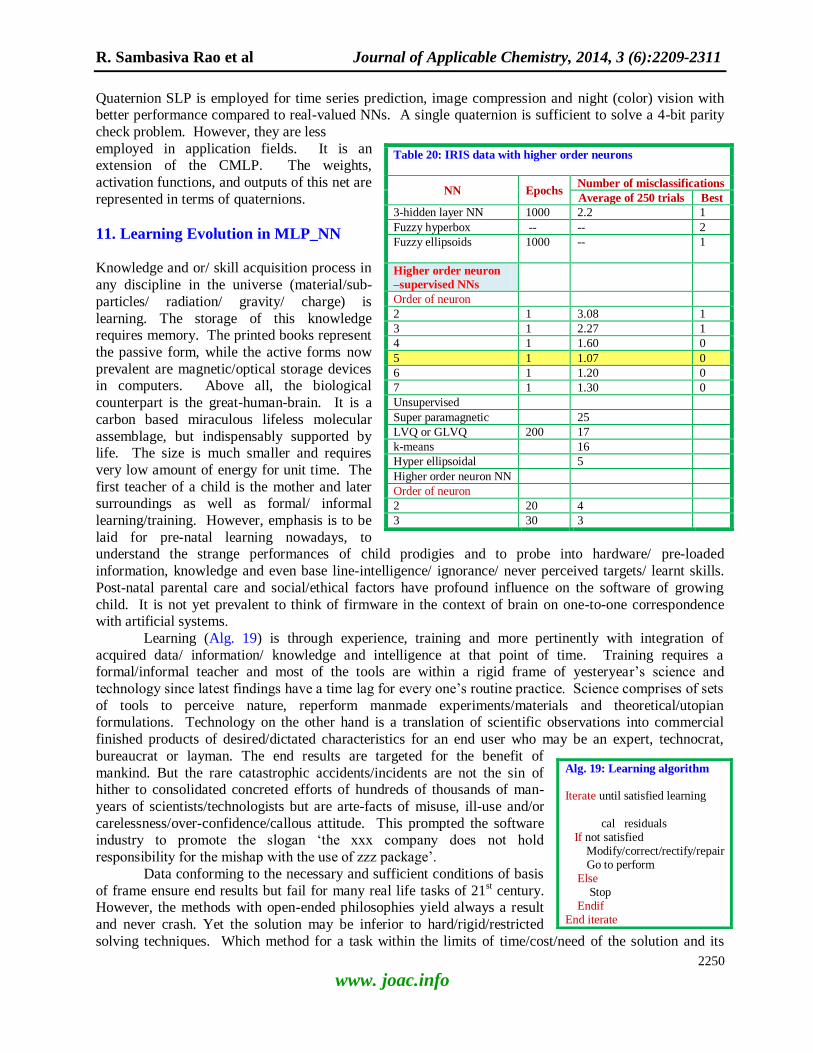
R. Sambasiva Rao et al Journal of Applicable Chemistry, 2014, 3 (6):2209-2311
2250
www. joac.info
Quaternion SLP is employed for time series prediction, image compression and night (color) vision with better performance compared to real-valued NNs. A single quaternion is sufficient to solve a 4-bit parity
check problem. However, they are less
employed in application fields. It is an extension of the CMLP. The weights,
activation functions, and outputs of this net are
represented in terms of quaternions.
11. Learning Evolution in MLP_NN Knowledge and or/ skill acquisition process in
any discipline in the universe (material/sub-
particles/ radiation/ gravity/ charge) is
learning. The storage of this knowledge requires memory. The printed books represent
the passive form, while the active forms now
prevalent are magnetic/optical storage devices in computers. Above all, the biological
counterpart is the great-human-brain. It is a
carbon based miraculous lifeless molecular
assemblage, but indispensably supported by life. The size is much smaller and requires
very low amount of energy for unit time. The
first teacher of a child is the mother and later surroundings as well as formal/ informal
learning/training. However, emphasis is to be
laid for pre-natal learning nowadays, to understand the strange performances of child prodigies and to probe into hardware/ pre-loaded
information, knowledge and even base line-intelligence/ ignorance/ never perceived targets/ learnt skills.
Post-natal parental care and social/ethical factors have profound influence on the software of growing
child. It is not yet prevalent to think of firmware in the context of brain on one-to-one correspondence with artificial systems.
Learning (Alg. 19) is through experience, training and more pertinently with integration of
acquired data/ information/ knowledge and intelligence at that point of time. Training requires a formal/informal teacher and most of the tools are within a rigid frame of yesteryear‘s science and
technology since latest findings have a time lag for every one‘s routine practice. Science comprises of sets
of tools to perceive nature, reperform manmade experiments/materials and theoretical/utopian formulations. Technology on the other hand is a translation of scientific observations into commercial
finished products of desired/dictated characteristics for an end user who may be an expert, technocrat,
bureaucrat or layman. The end results are targeted for the benefit of
mankind. But the rare catastrophic accidents/incidents are not the sin of hither to consolidated concreted efforts of hundreds of thousands of man-
years of scientists/technologists but are arte-facts of misuse, ill-use and/or
carelessness/over-confidence/callous attitude. This prompted the software industry to promote the slogan ‗the xxx company does not hold
responsibility for the mishap with the use of zzz package‘.
Data conforming to the necessary and sufficient conditions of basis
of frame ensure end results but fail for many real life tasks of 21st century.
However, the methods with open-ended philosophies yield always a result
and never crash. Yet the solution may be inferior to hard/rigid/restricted
solving techniques. Which method for a task within the limits of time/cost/need of the solution and its
Table 20: IRIS data with higher order neurons
NN Epochs Number of misclassifications
Average of 250 trials Best
3-hidden layer NN 1000 2.2 1
Fuzzy hyperbox -- -- 2
Fuzzy ellipsoids 1000 -- 1
Higher order neuron
–supervised NNs
Order of neuron
2 1 3.08 1
3 1 2.27 1
4 1 1.60 0
5 1 1.07 0
6 1 1.20 0
7 1 1.30 0
Unsupervised
Super paramagnetic 25
LVQ or GLVQ 200 17
k-means 16
Hyper ellipsoidal 5
Higher order neuron NN
Order of neuron
2 20 4
3 30 3
Alg. 19: Learning algorithm Iterate until satisfied learning
cal residuals If not satisfied Modify/correct/rectify/repair Go to perform Else Stop Endif End iterate

R. Sambasiva Rao et al Journal of Applicable Chemistry, 2014, 3 (6):2209-2311
2251
www. joac.info
utility/ returns is the best remains as a black hole. Self-efforts and self-styled/mimicked ways of doing things open a new world of realizing the truth for the benefit to himself/environment why to the galaxy.
It reminds the efforts of classical artificial intelligence practitioners of nineteen sixties in
developing a generalized problem solver, shaky robots and natural language processor. Many advances occurred over these four decades and the modules of AI-2 now are computational intelligence and nature-
mimicking computational tools with classical/hard mathematical/statistical algorithms for sub-goal
attainment without creeping of their ill effects. Learning specially related to RBF, SOM, ARTx,
ARTMAPx, RecurNNs etc. are detailed earlier [303-308] and Hebb learning is described now in appendix-A2a.
Emergent movements: Long duration memories as well as both positive and negative affections cooperate with each other. The increasing indefiniteness of environment is compensated in animals where the reflux
nerves cannot work efficiently. The experiences are contracted and used. It is suggested that local
reinforcement is responsible for simultaneous pursuit of stability and plasticity
State-of-the-art-of (SA) learning/Training (Salt)
Salt is essential for sustenance of life. Similarly learning and/or training of NNs to the desired accuracy is
the heart of I/O mapping. Just like excess salt is detrimental to health, overtraining/overlearning also models errors in data as information. Thus, an apparently better model for the naked eye of amateur, in
fact, functionally misleads compared to an inadequate model. The latter, of course, can be improved. The
ideal goal is landing on a good model for good_ data. The meta heuristics guide to cross over pits (bad_model for good_ data, good_model for bad_ data, and the worst possible bad_model for bad_ data)
on the way.
12. Training algorithms Evolution in MLP_NNs
Rumelhart proposed backward propagation (BP) as a means of self-learning of feed forward layered
neural networks (FF-MLP_NNs) [111]. In fact, BP is a gradient
based first order optimization method. Many modifications to BP
include delta-bar-delta, extended-delta, cumulative-delta etc. The momentum and learning coefficients also favor speedy
convergence. BPTT is an extension of BP for dynamic (in time)
NNs. Most of the efforts are in the direction of modifying back propagation (BP) algorithm and feasibility studies with the
available galaxy of optimization algorithms to train connecting
weights from input to hidden (WIH) and hidden to output (WHO) layers. These classical training
algorithms are non-self-starting. Therefore, one starts with guess (random numbers between –0.1 to +0.9) W(eight)s. Their optimum magnitudes for a given data set and architecture are obtained by choosing a
learning rule (W or parameter change) and optimization (training) algorithm.
Inter disciplinary research focusses vague/unclear/difficult aspects of grazy borderline/merging
point with unforeseen new directions and benefits of pure science. However, sometimes it is associated
with the menace of starting at lower end methods in one of the component fields especially in weaker of two disciplines coupled. SLP starting with steepest descent method missed the bus of well nurtured tools
of optimizations for over a decade or two. Further, the efforts were mostly to improve back-propagation
algorithm reported in hundreds of publications for many real life (tiny compared mega) tasks.
Almost all optimization methods viz. second order gradient procedures, quasi-Newton methods
(BFGS, Marquardt, CG), pseudo inverse and global stochastic optimization (SAA) and direct (Brent,
bisection) methods, non-gradient/global procedures viz. SAA, simplex have been implemented during the last two decades in refining even a large number of Ws. Kalman filter (KF), Extended KF, Dynamic-EKF
Chart 49: Limitations of BP
--- Slow
--- Trapped in local minima
--- Intractable for large-scale optimization
--- Cannot transform (rotation etc) of
profiles Remedy: Complex_ BP

R. Sambasiva Rao et al Journal of Applicable Chemistry, 2014, 3 (6):2209-2311
2252
www. joac.info
and their extensions are in routine use in training dynamic (in space or time) NNs. During the last ten years, the impact of nature inspired algorithms (E-man) is new phase of MLP research. The application
scientists carry the torch of well-established techniques and thus again a gap of quality of tools between
those practiced and available is also a natural trend. With the necessity of multiple-object functions and complex spacio-temporal systems, nature mimicking algorithms like GA, GP, EA, EP, ACA, PSO etc.
produced astounding results. A chronological survey of
typical improvements in basic BP and remedial measures
for the limitations (chart 49) are in appendix-A2b. RBF_NN trained with BP loses discriminating information
during the initial learning phase. But, it results in compact
representation. A panoramic view of evolution of training algorithm in MLP_NN is briefly discussed (vide infra).
Object function (objFn) The minimization of sum of squares of errors or residuals
(ESS) is the object function in training MLP_NN for fixed architecture. The training in NNs is generally performed
pattern wise like in on-line processing. All patterns are
propagated through NN in epoch. The output of Lth layer
is multiplied with the weights between layers L and L + 1 followed by operation with nonlinear activation function.
Sub set of patterns: A subset of patterns in a training set is selected based on retaining the patterns, which change the
Ws significantly [16]. In other words the data points,
which do not change weights, are not used or deleted in generating the training subset. This method
reduces the computational time and is employed in layer wise training. Layer wise training has higher complexity in terms of operations per iteration per pattern.
Classical training algorithms
Weight decay algorithm: Leung [21, 95] modified the weight decay algorithm of the recursive least
squares (RecurLS) procedure. In the first modification, weight decay remains constant throughout training
i.e. irrespective of epochs. It is more stable with high generalizability. The input perturbation RecurLS leads to robustness in prediction. These on line algorithms are tested for FF_NN.
Back-propagation with Selective training (BP-ST): BP-ST is faster than normal BP and de-emphasizes the over trained
patterns. Thus, it solved the shortcomings viz. slow convergence
towards the end of training, instability to learn the last few
patterns and prevents over training. However, contradictory or overlapping pattern pose a problem. Optimal scaling method
alternates between linear and non-linear optimization
procedures.
Removal of unimportant W from trained NNs: The Hessian
matrix identifies unimportant weights. In an on-line leaning, Hessian matrix is not available since the training patterns are
Eqns. 1: Object function and layer wise
output in MLP_NN
minobjFn ESS
1*
2*
*T
ESSNP
trace ynn y ynn y
1 *L L LY TF Y W
*OL OLyNN Y W
y: Observed response
yNN: NN output or (Calculated y)
OL: Last (i.e. output) layer
Chart 50: Advantages of complex-BP-
training of MLP_NN
Higher speed of convergence compared to real-valued BP
Generalization unchanged
Number of weights and thresholds required for complex_BP are 50% less than those for real-valued BP
Transform geometric figures, e.g. rotation,
similarity transformation and parallel displacement of straight lines, circles, etc

R. Sambasiva Rao et al Journal of Applicable Chemistry, 2014, 3 (6):2209-2311
2253
www. joac.info
stored after training. In this context, a joint learning-pruning algorithm is proposed for FFNNs. The basis is error covariance matrix of recursive least squares approach. It does not require the training set and
hence suitable for on-line training.
Complex BP: The positive features of complex-valued version of BP are described in chart 50. It is used to
train MLP_NN where input and output signals, weights and threshold values are all complex
numbers. The form of refinement approach is that probability for a ―standstill in learning‖ is very much
reduced.
Hybrid BP algorithms
B P + recursive orthogonal least-squares: A hybrid training procedure for type-2 fuzzy logic systems was
proposed. BP fine tunes antecedent and recursive orthogonal least-squares refines consequents. It is applied to
interval singleton, interval type-1 non-singleton, and interval type-2 non-singleton cases. MLP_NN with
geometric mean as accumulation function in neuron and resilent propagation training algorithm performs better
than BP / simple RPROP in accuracy/ CPU time for real life data sets.
BP + GA in Fuzzy_NN: The hybridization of GA with BP in Fuzzy_NN for seismic reservoir task was employed. It was applied to extract rules of optimal drill position in oil field exploration. The mfs of
antecedents and consequents are optimized making use of multi-encoding of GA. The first order predicate
logic based rules are pulled out from trained Fuzzy_NN. A linear combination of cross-entropy cost function with Humpert error function significantly improves BP learning. A few typical reports in
hybridizing BP with PSO, differential evolution, GA etc. are summarized in table 21.
Table 21: Hybridization of BP with nature inspired algorithms (E-man)
BP+$$$ Application Author
Diff.Evol Phase I: search for global initial connection weights & thresholds of BPNN with adaptive differential evolution (Adapt.Diff.Evol) Phase II: BPNN thoroughly searches for the optimal weights and thresholds.
Adapt.Diff.Evol >> [BPNN, ARIMA]
Computer-assisted colonoscopic detection of malignant regions
L Wang & G D Magoulas
GA GA
Initializes network connection weights and
thresholds of BP
PSO
Iterative refinement
Geological hazard risk
M Liu
PSO More accurate than hyperbolic and image models
local and global search
Soil–structure interaction involving a complicated mechanism of load transfer from pile to supporting geologic medium
A. Ismail
PSO o SLP_NN (BP) + ARIMA
o Input parameter Selection
Gansu of China from 2001 to 2006
Daily average wind speed data of Jiuquan and 6-hourly wind speed data of Yumen
C Ren
PSO
Preprocessing
Trend removal
BP
Weights (WIH & WHO) refinement
PSO
#hidden layer neurons
T Kuremoto

R. Sambasiva Rao et al Journal of Applicable Chemistry, 2014, 3 (6):2209-2311
2254
www. joac.info
Learning rates
Random
fuzzy
Accurate learning
Increases probability of escaping from the local minima
Y Chen
SA GA Tongue inspection color distortion
Table 21b: Output of om_ref_JAVATYP.m
Advances in back Propagation
A. Ismail, D.S. Jeng, L.L. Zhang An optimised product-unit neural network with a novel PSO–BP hybrid
training algorithm: Applications to load–deformation analysis of axially
loaded piles
Engineering Applications of Artificial Intelligence, 26, 10, (2013) 2305-2314
A. Sedki, D. Ouazar, E. El Mazoudi Evolving neural network using real coded genetic algorithm for daily
rainfall–runoff forecasting
Expert Systems with Applications, 36, 3, (2009) 4523-4527
Benedikt K. Humpert Improving back propagation with a new error function
Neural Networks, 7, 8, 1994, 1191-1192
C. Zhang, W. Wu, X.H. Chen, Y. Xiong Convergence of BP algorithm for product unit neural networks with
exponential weights
Neurocomputing, 72, 1–3 (2008) 513-520
C.C. Chuang, S.F. Su, C.C. Hsiao The annealing robust back propagation (BP) learning algorithm IEEE Trans. Neural Networks
11 (5) (2000) 1067–1077
Chao Ren, Ning An, Jianzhou Wang, Lian Li, Bin Hu, Duo Shang Optimal parameters selection for BP neural network based on particle
swarm optimization: A case study of wind speed forecasting
Knowledge-Based Systems, 56 (2014) 226-239
D.S. Chen, R.C. Jain A robust back-propagation learning algorithm for function approximation
IEEE Trans. Neural Networks 5(3) (1994) 467–479
El-Sayed A. El-Dahshan, Heba M. Mohsen, Kenneth Revett, Abdel-Badeeh M. Salem Computer-aided diagnosis of human brain tumor through MRI: A survey
and a new algorithm
Expert Systems with
Applications, 41, 11 (2014) 5526-5545
George D Magoulas, Vassilis P Plagianakos, Michael N Vrahatis Neural network-based colonoscopic diagnosis using on-line learning and
differential evolution
Applied Soft Computing, 4, 4, (2004) 369-379
Gerardo M. Méndez, M. de los Angeles Hernandez Hybrid learning for interval type-2 fuzzy logic systems based on orthogonal
least-squares and back-propagation methods
Information Sciences, 179, 13 ( 2009) 2146-2157
Li Zhuo, Jing Zhang, Pei Dong, Yingdi Zhao, Bo Peng An SA–GA–BP neural network-based color correction algorithm for TCM
tongue images
Neurocomputing, 13 (4) (2014) 111-116
Lin Wang, Yi Zeng, Tao Chen Back propagation neural network with adaptive differential evolution
algorithm for time series forecasting
Expert Systems with Applications,
(In Press)

R. Sambasiva Rao et al Journal of Applicable Chemistry, 2014, 3 (6):2209-2311
2255
www. joac.info
Lin Wang, Yi Zeng, Tao Chen Back propagation neural network with adaptive differential evolution
algorithm for time series forecasting
Expert Systems with Applications (In Press)
Md. Shiblee, B. Chandra, P.K. Kalra Learning of geometric mean neuron model using resilient propagation
algorithm
Expert Systems with Applications, 37, 12, (2010) 7449-7455
Ming Liu, Yude He, Jiaxin Wang, Heow Pueh Lee, Yanchun Liang Hybrid intelligent algorithm and its application in geological hazard risk
assessment
Neurocomputing, (In Press)
Muhammad R. Widyanto, Hajime Nobuhara, Kazuhiko Kawamoto, Kaoru Hirota, Benyamin Kusumoputro
Improving recognition and generalization capability of back-propagation NN using a self-organized network inspired by immune algorithm (SONIA)
Applied Soft Computing,
6, 1, (2005) Pages 72-84
Neil Vaughan, Venketesh N. Dubey, Michael Y.K. Wee, Richard Isaacs Parametric model of human body shape and ligaments for patient-specific
epidural simulation
Artificial Intelligence in Medicine, (In Press)
Shane D. Murnion Comparison of back propagation and binary diamond neural networks in the
classification of a Landsat TM image
Computers & Geosciences, 22, 9, (1996) 995- 1001
Sherif Khattab, Rami Melhem, Daniel Mossé, Taieb Znati Honeypot back-propagation for mitigating spoofing distributed Denial-of-
Service attacks
Journal of Parallel and Distributed Computing, 66, 9 (2006) 1152-1164
Shih-Wei Lin, Tsung-Yuan Tseng, Shuo-Yan Chou, Shih-Chieh Chen Simulated-annealing-based approach for simultaneous parameter
optimization and feature selection of back-propagation networks
Expert Systems with Applications,
34, 2, (2008) 1491-1499
Shiwei Yu, Xiufu Guo, Kejun Zhu, Juan Du A neuro-fuzzy GA-BP method of seismic reservoir fuzzy rules extraction
Expert Systems with Applications,
37, 3, (2010) 2037-2042
Takashi Kuremoto, Shinsuke Kimura, Kunikazu Kobayashi, Masanao Obayashi Time series forecasting using a deep belief network with restricted
Boltzmann machines
Neurocomputing, 137 ( 2014) 47-56
Yudong Zhang, Lenan Wu Stock market prediction of S&P 500 via combination of improved BCO
approach and BP neural network
Expert Systems with Applications, 36, 5, (2009) 8849-8854
Yu-Ju Chen, Tsung-Chuan Huang, Rey-Chue Hwang An effective learning of neural network by using RFBP learning algorithm
Information Sciences, 167, 1–4 (2004) 77-86
Zuriani Mustaffa, Yuhanis Yusof, Siti Sakira Kamaruddin Enhanced artificial bee colony for training least squares support vector
machines in commodity price forecasting
Journal of Computational Science,
5, 2 (2014) 196-205
13. Universal function approximation
Mathematically universal approximation theory was proved for any shape, of course restricted to certain class of basis functions (KB. 4). In NN paradigm, mathematical function approximation is proved with
sigmoid and Gaussian TFs [303]. But, recently several other basis functions viz. pseudo Gaussian, raised
cosine, ridge, binary cube, multi-wavelet with ortho normal multi scaling, multivariate functions (those with high input variability), smooth functions, Tickohnov regularization and clustering functions are
considered. The approximation of a continuous function is dense if
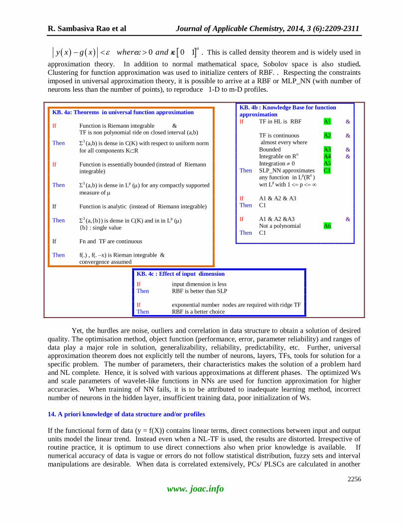
R. Sambasiva Rao et al Journal of Applicable Chemistry, 2014, 3 (6):2209-2311
2256
www. joac.info
y x g x 0 0 1 .n
where and x This is called density theorem and is widely used in
approximation theory. In addition to normal mathematical space, Sobolov space is also studied.
Clustering for function approximation was used to initialize centers of RBF. . Respecting the constraints
imposed in universal approximation theory, it is possible to arrive at a RBF or MLP_NN (with number of
neurons less than the number of points), to reproduce 1-D to m-D profiles.
KB. 4a: Theorems in universal function approximation
If Function is Riemann integrable & TF is non polynomial ride on closed interval (a,b)
Then 3 (a,b) is dense in C(K) with respect to uniform norm
for all components KR
If Function is essentially bounded (instead of Riemann
integrable) Then 3 (a,b) is dense in Lp () for any compactly supported
measure of
If Function is analytic (instead of Riemann integrable)
Then 3 (a,{b}) is dense in C(K) and in in Lp ()
{b} : single value If Fn and TF are continuous Then f(.) , f(. –x) is Rieman integrable & convergence assumed
KB. 4b : Knowledge Base for function
approximation
If TF in HL is RBF A1 &
TF is continuous almost every where
A2 &
Bounded A3 & Integrable on Rn A4 & Integration 0 A5
Then SLP_NN approximates any function in Lp(Rn )
wrt Lp with 1 p
C1
If A1 & A2 & A3 Then C1
If A1 & A2 &A3 & Not a polynomial A6 Then C1
KB. 4c : Effect of input dimension
If input dimension is less Then RBF is better than SLP
If exponential number nodes are required with ridge TF Then RBF is a better choice
Yet, the hurdles are noise, outliers and correlation in data structure to obtain a solution of desired
quality. The optimisation method, object function (performance, error, parameter reliability) and ranges of
data play a major role in solution, generalizability, reliability, predictability, etc. Further, universal approximation theorem does not explicitly tell the number of neurons, layers, TFs, tools for solution for a
specific problem. The number of parameters, their characteristics makes the solution of a problem hard
and NL complete. Hence, it is solved with various approximations at different phases. The optimized Ws and scale parameters of wavelet-like functions in NNs are used for function approximation for higher
accuracies. When training of NN fails, it is to be attributed to inadequate learning method, incorrect
number of neurons in the hidden layer, insufficient training data, poor initialization of Ws.
14. A priori knowledge of data structure and/or profiles
If the functional form of data (y = f(X)) contains linear terms, direct connections between input and output
units model the linear trend. Instead even when a NL-TF is used, the results are distorted. Irrespective of routine practice, it is optimum to use direct connections also when prior knowledge is available. If
numerical accuracy of data is vague or errors do not follow statistical distribution, fuzzy sets and interval
manipulations are desirable. When data is correlated extensively, PCs/ PLSCs are calculated in another

R. Sambasiva Rao et al Journal of Applicable Chemistry, 2014, 3 (6):2209-2311
2257
www. joac.info
NN and used as input for I/O transformation. In the case of time series, if linear trends are established for similar tasks, the residuals of ARMA output are connected to the input layer of MLP_NN. In cases
where the periodicity is known from other studies, FFT is a good choice in pre-processing. The dynamics
in parameter values of model and structural change are taken care in Kalman filter and its clones.
15. Emulation of standard statistical/ mathematical techniques by SLP_NNs
The classification of methods based on data structure are given in the form of if-then-else rules in KB. 5.
FF-NN for linearly equivalent separable classification task is equivalent to support vector machines
(SVM). In the first few epochs, it mimics SVM and then classifies clusters with non-linear separation boundaries. The hardness of the margin in SVM is correlated with the number of epochs of back
propagation algorithm. The knowledge in calculating principal components with IO_NN and SLP_NN are
documented in KB. 6.
KB. 5: Classification method selection based
on data structure Necessary Condition
Number of clusters known
If Number of classes = 2 &
pdf1, pdf2 are Gaussian & cov(c1) = cov(c2) Then Fisher linear discriminant analysis (LDA) If pdf1, pdf2 are Gaussian & cov(c1) ≠ cov(c2) & Then Quadratic Bayesian classifier (QDA)
If Nature of distribution (pdf) is non Gaussian
Then non-parametric (Parzen estimator)
Cov : Covariance
pdf : Probability density function
KB. 6: Output characteristics based
on relative number of input and
hidden neurons in SLP_NN
If SLP_NN &
I# = O# Then Non-linear PCs
If SLP_NN &
I# > H# Then Dimension reduction
If SLP_NN &
H# > >I# Then Mapping into high dimensional space
[Similar to SVM]
If Response output is constant over a certain region
Then Increase number of sigmoid functions
- CPU time increases with H#
Remedy
Hypersphere FAM
R_RBF_NN
Chart 29b: Output of om_ref_JAVATYP.m
Principal component Analysis (PCA) Erkki Oja
A Simplified neuron model as a principal component analyzer J. of Mathematical Biology
15(3) (1982) 267–273
Erkki Oja
Neural Networks, Principal Components and Subspaces
International J. of Neural Systems
1 (1) (1989) 61–68
N. Japkowicz, S.J. Hanson, M.A. Gluck
Non-linear autoassociation is not equivalent to PCA
Neural computation
12 (2000)531-545
om_ref_JAVATYP.m
object module (om_ ) reference (ref_)

R. Sambasiva Rao et al Journal of Applicable Chemistry, 2014, 3 (6):2209-2311
2258
www. joac.info
Journal Author Volume And (JAVATYP) Title Year Pages
matlab function(.m)
Posterior probability
Ito and Srinivasan [7] applied Bayesian decision theory for SLP_NN. A way of obtaining posterior probabilities for classification tasks from the output of SLP_NN are described in the first order logic
format in KB.7.
KB. 7a: Output of SLP and probability
If Number_of_classes = 2 & Number_of _hidden_ neurons of SLP = dimX
Then Output approximates to posterior probability If Number_of_classes = 2 &
d-dimensional space adheres to binomial,
Poisson, multi-nominal state conditional probability distribution
Then d-hidden neurons approximate posterior probability of data set.
If Number_of_classes = 2 &
MLP with small number of hidden neurons & NN trained with Rucket method &
normal state-conditional probability distribution Then Output approximates to a posterior probability Extension : It is applicable to d-dimensional
feature space
If Inner potential of the output unit approximates log ratio & Activation function is logistic
Then Output approximates posterior probability
KB. 7b: Output of SLP and probability
If Log ratio of posterior probabilities linear & d#-1 architecture
Then log (ratio of posterior distribution) = u0 * x + a0 = u01*x1 + … + u0d * xd + u0
If log (ratio of posterior distribution) is quadratic &
d-nonlinear hidden layer neurons & d-linear inputs and direct connections between input-to-output layers
Then NN output cannot estimate state conditional pdfs Remedy If prior knowledge (or
measurement during training) of density p(x) is available
Then probability distribution is
obtained as the product
If Log ratio of posterior probabilities is polynomial of low degree & Sigmoid TF is used
Then SLP approximates posterior probabilities of multiple (two or more) class data
Chart 29b: Output of om_ref_JAVATYP.m
Posteriori probability B.D. Ripley
Statistical aspect of neural networks, in: O.E. Bardorff-Nielsen, et al. (Ed.), Networks and Chaos—Statistical and Probabilistic Aspects
Chapman & Hall, London, 1993, pp. 40–123.
B.D. Ripley Statistical aspect of neural networks, in: O.E. Bardorff-Nielsen, et al.
(Ed.), Networks and Chaos—Statistical and Probabilistic Aspects
Chapman & Hall, London, 1993, pp. 40–123.
M.D. Richard, R.P. Lipmann Neural networkclassifiers estimate Bayesian a posteriori probabilities
Neural Comput. 3 (1991) 461–483
M.D. Ruck, S. Rogers, M. Kabrisky, H. Oxley, B. Sutter The multilayer perceptron as an approximator to a Bayes optimal
discriminant function
IEEE Trans. Neural Networks 1 (1990) 296–298
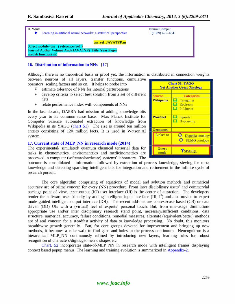
R. Sambasiva Rao et al Journal of Applicable Chemistry, 2014, 3 (6):2209-2311
2259
www. joac.info
H. White Learning in artificial neural networks: a statistical perspective
Neural Comput. 1 (1989) 425–464.
om_ref_JAVATYP.m
object module (om_ ) reference (ref_)
Journal Author Volume And (JAVATYP) Title Year Pages
matlab function(.m)
16. Distribution of information in NNs [17]
Although there is no theoretical basis or proof yet, the information is distributed in connection weights
between neurons of all layers, transfer functions, cumulative
operators, scaling factors and so on. It helps to probe into
estimate tolerance of NNs for internal perturbations
develop criteria to select best solution from a set of different
nets
relate performance index with components of NNs
In the last decade, DAPRA had mission of adding knowledge bits
every year to its common-sense base. Max Planck Institute for Computer Science automated extraction of knowledge from
Wikipedia in its YAGO (chart 51). The size is around ten million
entries consisting of 120 million facts. It is used in Watson AI
system.
17. Current state of MLP_NN in research mode (2014) The experimental/ simulated/ quantum chemical tensorial data for
tasks in chemometrics, enviromentrics and medicinometrics are
processed in computer (software/hardware) systems‘ laboratory. The outcome is consolidated information followed by extraction of process knowledge, sieving for meta
knowledge and detecting sparkling intelligent bits for integration and refinement in the infinite cycle of
research pursuit.
The core algorithm comprising of equations of model and solution methods and numerical
accuracy are of prime concern for every (NN) procedure. From inter disciplinary users‘ and commercial
package point of view, input output (IO) user interface (UI) is the center of attraction. The developers render the software user friendly by adding intelligent input interface (III, I
3) and also novice to expert
mode guided intelligent output interface (IOI). The recent add-ons are context/case based (CB) or data
driven (DD) UIs with a (virtual) feel of experts‘ personal touch. But, from mis-usage diminution/ appropriate use and/or inter disciplinary research stand point, necessary/sufficient conditions, data
structure, numerical accuracy, failure conditions, remedial measures, alternate (equivalent/better) methods
are of real concern for a steadfast activity of data to knowledge processing. No doubt, this monitors
breadthwise growth generally. But, for core groups devoted for improvement and bringing up new methods, it becomes a cake walk to find gaps and holes in the process-continuum. Neocognitron is a
hierarchical MLP_NN continuously refined by introducing new layers, learning rules for robust
recognition of characters/digits/geometric shapes etc. Chart. 52 incorporates state-of-MLP_NN in research mode with intelligent frames displaying
context based popup menus. The learning and training evolution is summarized in Appendix-2.
Chart 51: YAGO
Yet Another Great Ontology
Source Categories
Wikipedia Categories
Redirects
Infoboxes
Wordnet Synsets
Hyponymy
Geonames
Linked to Dbpedia ontology
SUMO ontology
Query
mode ? SPARQL

R. Sambasiva Rao et al Journal of Applicable Chemistry, 2014, 3 (6):2209-2311
2260
www. joac.info
Chart 52: State-of-art-of- FF_MLP_NN in research mode
Intelligent input interface (III, I3)
Number of hidden layers and neurons (#HLn )
#Neurons in HL1
If #HL > 0 &
#HL =1
Then SLP
Default : [1]
dimX
rand_int([1 to NP]
custom[User_chosen] neurons_HL(1):
#HL > 0
#HL > 1
Hidden
Layers
Default
: [1]
0
2
#Neurons in HL2
MLP
If #HL > 1
Default : [1]
dimX
rand_int([1 to NP]
custom[User_chosen] neurons_HL(2):
#HL = 0
IO_NN
If #HL = 0
Then IO_NN
neurons_HL(0): [0]
Transfer functions
TFs _Fnbase
Real
Complex
Quaternion
Real .TFs
Continuous
Discrete
Real . Discrete.
TFs
Hardlimitor
Rectangular
…
Real .continuous.
TFs
Sigmoid
Tanh
Elliot
…
Object functions

R. Sambasiva Rao et al Journal of Applicable Chemistry, 2014, 3 (6):2209-2311
2261
www. joac.info
ObjFn
Single
Multiple Standard
Pareto
ObjFn
Unconstrained
Constrained
…..
Goal
Minimization
Maximization
….
Learning /Training methods
Inhibitory.
Learning.
Ws
Fixed
Variable
No surround
Surround
Excitatory
Fixed
Variable
……..
Learning /training
Ws
Architecture
Both
Winner.
learning.
Ws
Winner-takes-most
Winner-take-all
Winner-kills-looser
…
Loser.
learning.
Ws
Winner-kills-looser
Loser-exits
Achieve
…
Winner-Loser Interaction.
Learning.
Ws
crossover
Mutation
Elite Retention
Avoiding
Looser deficiencies
Elimination
Remedial measures
…..
Silent.
learning.
Ws
Add-if-silent
Ignore-if-silent
Eliminate-if -silent
Learned.
Learning.
Ws
Learned Robustly accepted Retain
Deformed
unlearned
Robustly accepted
Irrelevant Erroneously accepted To be rejected
Training. Ws
Back-propagation
LM
Pseudo inervse
….
18. Future scope
R. Sambasiva Rao et al Journal of Applicable Chemistry, 2014, 3 (6):2209-2311
2262
www. joac.info
Neuron_2020 The set of neurons proposed over last half a century are not even nearer to biological neurons of brain,
although many complex dynamic real life tasks have been predicted with astounding success compared to
statistical/mathematical paradigms. FF-NNs with TF-based neurons excelled in performance in function approximation, classification, parameterization, solution of algebraic/differential equations of multivariate-
multidimensional complex hyper-surfaces. Support vector machine neuron (SVM_neuron) is a new
addition to the list of neurons.
Neuron with glial cell
The small, but neglected influence of glial cells, astrocytes in biological neurons is now a matter concern.
The neuron model incorporating complete effect of biological glial cells and astrocytes is awaited. It is interesting to foresee the gross influence of such smaller and analogous effects in artificial neurons.
Another approach enhancing machine intelligence is using fuzzy logic through computation of words,
sentences and concepts. Early attempts of flying machines attempted to model the bird. This was done because the bird
was the only working model of flight in those days. It was not until Wilbur and Orville Write chose an
alternate model of nature. The first aircraft created was that with first fixed wings. Perhaps modeling AI
programs after nature analogous to modeling airplanes after birds and a much better model than the neural network exists. One had to wait for a fairy tide in future. Alternatively, leaving aside the idea of
mimicking biological neurons with ion channels and complex interactions, a new basic structure with
higher accumulated wisdom will open new vistas in intelligent computation or computational intelligence. This will be at the base level as a building block to explore machine intelligence from another direction.
An integrated form and research mode of TF-based neuron is a comprehensive model accepting
tensorial input and capable of operating with Clifford geometry. Dynamic neuron incorporating feedback
signals with single/multiple delays in distributed/undistributed form paved the way to the state of art modeling of spacio-temporal variations of numerical data, image processing, dynamic scene analysis etc.
A single super-neuron/hyper-neuron along with strengthened weight estimation procedures is a step
forward to realize multi-objective real time/real life tasks in environment, drug discovery and electronic industry including nano-structures in civilian/defense sectors. The miraculous sparkles of computational
thinking of 2020 will enable one to compute nearer if not nearest to the normal healthy human brain.
Acknowledgments: The authors thank editor-in-chief and executive editor for improving the readability of this series of neural network reviews.
I (RSR) bow my head to my first teacher who laid foundation stone of formal learning. I remember
vividly majestic gesture of Sri Subba Rao, for taking pains to induce systematic approach of learning (now
I understand) in fourth and fifth classes at elementary school, Vijayawada in late nineteen fifties. I place on record my profound gratitude to my teachers Smt.Eligebeth, Smt Padmavati, Sri Kesava Rao and Sri
Bhavani who generously infused curiosity and paved way to learn alphabets in general
science/mathematics at C V R (Chunduru Venkata Reddi) GMH (Government municipal high) school, Vijayawada in early sixties. I learnt basics of physics, chemistry, mathematics and languages from learned
lecturers, K Rama Krishna, Moses, Vijaya Kumar, S S S Somayajulu, Mohan, Prajapathi Rao, N Radha
Krishana Murthy, Khasim Peeran, Bhavannarayana, Kedareswara Rao, Raghavachari (Hofined professor), Subrahmanyam, Narasimham and Jamadagni at SRR (Sri Raja Rangayya Appa Rao) & CVR Govt.
college, Vijayawada in late sixties. I feel at heart overwhelming happiness to express my gratitude to Sri
Lakshminarayana garu for sparing time in 1968 amidst his busy schedule for vocal practice of
Rudradhayam in Yajur veda with his reverberating metallic voice.
The wise counseling of Prof. S R Sagi, Prof. L S A Dikshitulu, Prof. Manta Suryanarayana, Prof.
N Venkateswara Rao, Prof. L Rama Chandra Rao, Prof. C Bheema Sankara Rao, Prof.A S R Anjaneyulu in lecture halls and laboratories of Andhra University (1969-1971) widened my vocabulary in chemistry.
My regards to Prof Gandikota Gopala Rao for showering on me the bliss of hearing to him long hours in

R. Sambasiva Rao et al Journal of Applicable Chemistry, 2014, 3 (6):2209-2311
2263
www. joac.info
his office in physical chemistry during mid-seventies. I thank Gandikota Murali Krishna for sparing many reprints in analysis of redox systems.
I am ever indebted to Dr. Lakshmi Kantam (Director), Dr. Sai Prasad, Dr. Narahari Sastry
(Bhatnagar awardee), Dr. Bhanu Prakash, scientists at I I C T for generously permitting online search and downloading of electronic prime journals since 2000.
The print versions of chemical abstracts/journals up to nineteen nineties, CD_ROMs in late
nineties, online services of Science Direct, ACS, RSC etc. with keywords searches in this century and
cover to cover browsing, downloaded papers/focus articles/ state-of-art-(critical)-reviews from e_journals are instrumental to integrate knowledge both breadth and depth wise. The referees and editors of journals
polished the critical perspective of translation of outcome of designed experiments along with
consolidation of literature with ethics to a presentable form.
References
Multi-layer perceptron (MLP)_NN
[1] M. A. Costa, A. de Pa du Braga, B. R. de Menezes, NeuroComput., 2007, 70, 1342-1347.
[2] C. Yu, M.T. Manry, J. Li, P. L. Narasimha, NeuroComput., 2006, 70, 525-535.
[3] E. R. Hruschka, N. F.F. Ebecken, NeuroComput., 2006, 70, 384-397. [4] L. Franco, NeuroComput., 2006, 70, 351-361.
[5] S. K. Oh, W. rycz, Ho-Sung Park, NeuroComput., 2005, 64, 397-431.
[6] M. Ghiassi, H. Saidane, NeuroComput., 2005, 63, 397-413. [7] Y. Ito, C. Srinivasan, NeuroComput., 2005, 63, 209-228.
[8] J. Wang, Z. Tang, R. Wang, NeuroComput., 2004, 57, 485-492.
[9] R. K. Brouwer, NeuroComput., 2004, 57, 345-360. [10] E. Romero, L. Marquez, X. Carreras, NeuroComput., 2004, 57, 313-344.
[11] P. Guo, M. R. Lyu, NeuroComput., 2004, 56, 101-121.
[12] K. P. Ferentinos, Neural Netw., 2005, 18, 934-950.
[13] A. Eleuteri, R. Tagliaferri, L. Milano, Neural Netw., 2005, 18, 1309-1318. [14] J. Gary Polhill, M. K. Weir, Neural Netw., 2001, 14, 1035-1048.
[15] M. Lehtokangas, Neural Netw., 2000, 13, 525-531.
[16] S. D. Hunt, J. R. Deller Jr., Neural Netw., 1995, 8, 6, 931-944. [17] Ali A. Miani, R. D.Williams, Neural Netw., 1994, 7, 5, 783-796.
[18] T. Karkkainen, Neural comput., 2002, 14, 1451-1480.
[19] L. S. Camargo, T. Yoneyama, Neural comput., 2001, 13, 2673-2680. [20] A. W. Savich, M. Moussa, S. Areibi, IEEE Trans. Neural Netw.,2007, 18, 1,240-252.
[21] Chi-Sing Leung, Ah-Chung Tsoi, Lai Wan Chan, IEEE Trans. Neural Netw.,2001, 12(6), 1314-1332.
[22] E. J. Bayro-Corrochano, IEEE Trans. Neural Netw.,2001, 12, 5, 968-986.
[23] J. V. Shah, C. S. Poon, IEEE Trans. Neural Netw.,1999, 10, 1,10-18. [24] M. Banerjee, S. Mitra, S. K. Pal, IEEE Trans. Neural Netw.,1998, 9, 6, 1203.
[25] D. Svozil, V. Kvasnicka, J. Pospichal, Chemometrics and Intelligent Laboratory Systems, 1997, 39,
43-62.
Back propagation [26] B. Widrow, Proc. IEEE, 1990, 78, 9,1415-1442.
[27] X.G. Wang, Z. Tang, H. Tamura, M. Ishii, NeuroComput., 2004, 57, 477-484. [28] X. G. Wang, Z. Tang, H. Tamura, M. Ishii, W.D. Sun, NeuroComput., 2004, 56, 455- 460.
[29] A. Bhaya, E. Kaszkurewicz, Neural Netw., 2004, 17, 65-71.
[30] A. Nikov, S. Stoeva, Neural Netw., 2001, 14, 231-244. [31] S. Stroeve, Neural Netw., 1998, 11, 709-721.
[32] D. McLean, Z. Bandar, J. D. O. Shea, Neural Netw., 1998, 11, 1685-1694.

R. Sambasiva Rao et al Journal of Applicable Chemistry, 2014, 3 (6):2209-2311
2264
www. joac.info
[33] B. K. Humpert, Neural Netw., 1994, 7, 8, 1191-1192. [34] K. Niahiyma, K Suzuki IEEE Trans. Neural Netw., 2001, 12(6), 1265-1277.
[35] C. C. Chuang, S. F. Su, C. C. Hsiao, IEEE Trans. Neural Netw.,2000, 11, 5, 1067-1077
[36] J. S. R Jang, IEEE Trans. Neural Netw.,1992, 3, 5, 714-716. [37] M. Fukumi, S. Omatu, IEEE Trans. Neural Netw., 1992, 3, 5, 535-537.
[38] S. ichiHorikawa, T. Furuhashi, Y. Uchikawa, IEEE Trans. Neural Netw., 1992, 3, 1, 801-806.
[39] R.C.Lacher, S. I. Hruska, D. C.Kuncicky, IEEE trans. Neural netw.,1992, 3, 1, 62-72.
[40] L. Holmstorm, P. Koistinen, IEEE Trans. Neural Netw.,1992, 3, 1, 24-35.
Learning algorithms [41] H. Yang, J. Li, F. Ding, NeuroComput., 2007, 70, 625-632.
[42] J. Hirayama, J. Yoshimoto, S. Ishii, NeuroComput., 2006, 69, 1954-1961.
[43] Y. Nishimori, S. Akaho, NeuroComput., 2005, 67, 106-135. [44] Wako Yoshida, Shin Ishiia, NeuroComput., 2005, 63, 253-269.
[45] B. Ster, NeuroComput., 2004, 57, 215- 238.
[46] V. G. Red‘ko, O. P. Mosalov, D. V. Prokhorov, Neural Netw., 2005, 18, 738-745.
[47] A. V. Robins, S. J. R. McCallum, Neural Netw., 2004, 17, 313-326. [48] H. Miyamoto, J. Morimoto, K. Doya, M. Kawato, Neural Netw., 2004, 17, 299-305.
[49] K. Hara, M. Okada, Neural Netw., 2004, 17, 215-223.
[50] B. J. Jain, F. Wysotzk, Neural Netw., 2004, 17, 143-154. [51] S. Sakamoto, S. Seki, Y. Kobuchi, Neural Netw., 2004, 17, 1101-1107.
[52] T. Kimoto, M. Okada, Neural Netw., 2004, 17, 103-112.
[53] K. Hirasawa, S. ho kim, J. Hu, J. Murata, M. Han, C. jin, Neural Netw., 2001, 14, 1389-1404.
[54] N. Ampazis, S. J. Perantonis, J. G. Taylor, Neural Netw., 2001, 14, 1075-1088. [55] S. Watanabe, Neural Netw., 2001, 14, 1049-1060.
[56] D. Ormoneit, Neural Netw., 1999, 12, 1405-1412.
[57] Y. Liu, X. Yao, Neural Netw., 1999, 12, 1399-1404. [58] K. Yamauchi, M. Oota, N. Ishii, Neural Netw., 1999, 12, 1347-1358.
[59] K. Chena, L. Xu, H. Chi, Neural Netw., 1999, 12, 1229-1252.
[60] J. Zhang, A. J. Morris, Neural Netw., 1998, 11, 1, 65–80. [61] Fu. L. chung, T. lee, Neural Netw., 1996, 7, 3, 539-551.
[62] R. Vitthal, P. Sunthar, Ch. D. Prasad rao, Neural Netw., 1995, 8, 4, 563-569.
[63] H. Yamakawa, Y. OkAbe, Neural Netw., 1995, 8, 3, 363-373.
[64] S. J. Perantonis, D. A. Karras, Neural Netw., 1995, 8, 2, 237-249. [65] W. Bialek, I. N. N. Tishby, Neural Netw., 1994, 7, 9, 1351-1378.
[66] K. Ochiai, N. Toda, S. Usui, Neural Netw., 1994, 7, 5, 797-807.
[67] V. Kasparian, C. Batur, H. Zhang, J. Padovan, Neural Netw., 1994, 7, 4, 661-670. [68] E. Castillo, O. F. Romero, B. G. Berdinas, A. A. Betanzos, Neural comput., 2002, 14, 1429-1449.
[69] M. Ishii, I. Kumazawa, Neural comput., 2001, 13, 2851-2863.
[70] H. Gu, H. Takahashi, Neural comput., 2000, 12, 795-809. [71] H. SchWenk, Y. Bengio, Neural comput., 2000, 12, 1869-188.
[72] A. N. Vazquez, A. R. F. Vidal, Neural comput., 2000, 12, 1429-1447.
[73] A. Goltsev, Neural computati on, 2004, 62, 405-426.
[74] Y. Wang, B. Samson, D. Ellison, L. Natanson, Neural Comput & Applic., 2001, 10, 253-263. [75] B. Apolloni, A. Esposito, D. Malchiodi, C. Orovas, G. Palmas, J. G. Taylor, IEEE Trans. Neural
Netw.,2004, 15, 6.
[76] J. V. Gorp, R. Pintelon, IEEE Trans. Neural Netw.,2000, 11, 2, 402-414. [77] M. L. Wong, K. S. Leung, IEEE Trans. Evolut. Comput., 2004, 8, 4, 378-404.
[78] G. A. Jamieson, K. j. Vicente, Comput. Chem. Eng., 2001, 25 1055-1074.
[79] N.R. Sakthivel, V. Sugumaran, Binoy B. Nair Appl. St Comput., 2012, 12 (1), 196-203.

R. Sambasiva Rao et al Journal of Applicable Chemistry, 2014, 3 (6):2209-2311
2265
www. joac.info
[80] Yoon-Seok Timothy Hong Journal Hydrology, 2012, 468–469, 11-21. [81] Chao Shang, Fan Yang, Dexian Huang, Wenxiang Lyu J. Process Control, 2014, 24 (3), 223-233.
[82] J. Martínez, M. López, J.M. Matías, J. Taboada Math. Comput. Model., 2013 57 (7–8), 1716-1721.
[83] Sanjeev S. Malalur, Michael T. Manry, Praveen Jesudhas NeuroComput., 2014. [84] Michael Georgiopoulos, Cong Li, Taskin Kocak Performance Evaluation,2011, 68 (4), 361-384.
Training methods [85] J. Xua, D. W.C. Hob, NeuroComput., 2006, 70, 544-558.
[86] A. D. Anastasiadis, G. D. Magoulas, M. N. Vrahatis, NeuroComput., 2005, 64, 253-270.
[87] Uro. S. Lotri, NeuroComput., 2004, 62, 179-196. [88] P. Chandra, Y. Singh, NeuroComput., 2004, 61, 429- 437.
[89] O. Giustolisi, NeuroComput., 2004, 56, 285-304.
[90] T. W. S.Chow, Y. Fang, NeuroComput., 2000, 30, 333-337. [91] J. A. Drakopoulos, A. Abdulkader, Neural Netw., 2005, 18, 595-601.
[92] E. M. Callaway, Neural Netw., 2004, 17, 625-632.
[93] L. Ma, K. Khorasani, Neural Netw., 2004, 17, 589-609.
[94] S. Draghici, Neural Netw., 2001, 14, 527-550. [95] Chi-Sing leung, Kwok-Wo wong, Pui-Fai Sum, Lai-Wam Chan, Neural Netw., 2001, 14, 147-174.
[96] K. Hagiwara, T. Hayasaka, N.Toda, S. Usui, K. kuno, Neural Netw., 2001, 14, 1419-1429.
[97] C. dang, Neural Netw., 2000, 13, 801-810. [98] K. M. Adeney, M. J. Korennerg, Neural Netw., 2000, 13, 787-799.
[99] S. J. Perantonis, V. Virvilis, Neural Netw., 2000, 13, 351-364.
[100] G. Zhou, J. Si, Neural Netw., 1999, 12, 79-89.
[101] S.V. Kamarthi, S. Pittner, Neural Netw., 1999, 12, 1285-1299. [102] R. Lengelle, T. denceux, Neural Netw., 1996, 9, 2, 83-87.
[103] M. plutowski, G. Cottrell, H. White, Neural Netw., 1996, 9, 2, 273-294.
[104] S. Ishii, K. Fukumizu, S. Watanabe, Neural Netw., 1996, 9, 1, 25-40. [105] S. D. Hunt, J. R. Deller Jr, Neural Netw., 1995, 8, 6, 931-944.
[106] J. W. Andgary, G. R. Green, Neural Netw., 1995, 8, 1, 31-37.
[107] P. Patrick van der Smagt, Neural Netw., 1994, 7, 1, 1-11. [108] E. Hartman, Neural comput., 2000, 12, 811-829.
[109] Y. Bengio, Neural comput., 2000, 12, 1889-1900.
[110] K. Ahmad, B. L. Vrusias, A. Ledford, Neural Comput & applic., 2001, 10, 56-66.
[111] P. K. H. Phua, D. Ming, IEEE Trans. Neural Netw.,2003, 14, 6, 1460-1468. [112] J. A. K. Suykens, J. Vandewalle, IEEE Trans. Neural Netw.,1999, 10, 4.
[113] L. M. Reyneri, IEEE Trans. Neural Netw.,1999, 10, 4.[114] M. H. Choueiki, C. A. M. Campbell,
IEEE Trans. Neural Netw.,1999, 10, 1, 56-63. [115] A. Savich, M. Moussa, S. Areibi, Microprocessors and Microsystems, 36 (2), 2012, 138-150.
Applications [116] V. Nourani, M. S. Fard, Adv. Eng. Software,2012, 47 (1), 127-146.
[117] M. Akhoondzadeh, Adv. Space Research, 2013, 51 (11), 2048-2057.
[118] A. P. Piotrowski, J. J. Napiorkowski, Adv. Water Resources,2012, 49, 97-113.
[119] M. Hayati, B. Akhlaghi, AEU – Int. J. Electronics Com., 2013, 67 (2), 123-129. [120] S. Sasikala, S. Appavu alias Balamurugan, S. Geetha, Appl. Comput. Informatics,2014 (in press).
[121] C.Voyant, C. Darras, M. Muselli, C. Paoli, M. L. Nivet, P. Poggi, Appl. Energy, 2014, 114, 218-226.
[122] A. Marvuglia, A. Messineo, Appl. Energy, 2012, 98, 574-583. [123] A. R. Tahavvor, M. Yaghoubi, Appl. Math. Model., 2012, 36 (7), 3176-3188.
[124] B. Vahdani, S.H. Iranmanesh, S. M. Mousavi, M. Abdollahzade, Appl. Math. Model., 2012, 36 (10),
4714-4727.

R. Sambasiva Rao et al Journal of Applicable Chemistry, 2014, 3 (6):2209-2311
2266
www. joac.info
[125] D. Ren, Mao. Ye, Appl. Math. Comput., 2012, 218 (9), 5726-5738. [126] E. Kolay, T. Baser, Appl. Soft. Comput., 2014, 18, 223-231.
[127] V. M. Janakiraman, X. Nguyen, D.Assanis, Appl. Soft. Comput.,2013, 13 (5), 2375-2389.
[128] S. Rampone, Appl. Soft. Comput., 2013, 13 (10), 4077-4086. [129] J. Sanz, R. Perera, C. Huerta, Appl. Soft Computing, 2012, 12 (9), 2867-2878.
[130] A. E. Sherme, Appl. Soft. Comput.,2012, 12 (1), 453-461.
[131] N. N. Charniya, S. V. Dudul, Appl. Soft. Comput.,2012, 12 (1), 543-552.
[132] S. Polak, B. Wiśniowska, M. Ahamadi, A. Mendyk, Appl. Soft. Comput., 2011, 11 (2), 2611-2617. [133] A. Wefky, F. Espinosa, A. Prieto, J.J. Garcia, C. Barrios, Appl. Soft. Comput., 2011,11(4), 3580-
3599.
[134] A. Azadeh, Z.S. Faiz, Appl. Soft. Comput., 2011, 11 (1), 614-620. [135] M. M. Etghani, M. H. Shojaeefard, A. Khalkhali, M. Akbari, Appl. Thermal Eng.,2013, 59 (1–2),
309-315.
[136] J. Yang, H. Singh, E. L. Hines, F. Schlaghecken, D. D. Iliescu, M. S. Leeson, N. G. Stocks, Art. Intel. Med.2012, 55 (2), 117-126.
[137] A. P. Balsamà, L. De Biase, G. J. Maenhout, V. Pagliari, Atmospheric Env., 2014,89, 581-592.
[138] J. H. Chen, M. C. Su, C. Yi. Chen, Fu-H. Hsu, C. C. Wu, Automation in Construction,2011, 20 (7),
935-939. [139] S. Sharma, S. S. Tambe, Biochem. Eng. J.,2014, 85, 89-100.
[140] M. F. Abbod, K. Y. Cheng, X. R. Cui, S. J. Huang, Y. Yi Han, J. S. Shieh, Biomed. Signal
Processing Control, 2011, 6 (4), 414-421. [141] E. T. Borroto, C. G. P. Rivas, J. C. V. Chagoyán, N. Castañedo, F. J. Prado-Prado, X. G. Mera, H. G.
Díaz, Bioorganic & Med. Chem.,2012, 20 (20), 6181-6194.
[142] E. V. Suprun, A. A. Saveliev, G. A. Evtugyn, A. V. Lisitsa, T. V. Bulko, V. V. Shumyantseva, A. I.
Archakov, Biosensors Bioelectronics, 2012,33(1), 158-164. [143] G. S. Gill, A. Kumar, R. Agarwal, Biosys. Eng., 2013, 116 (2), 198-204.
[144] M.A. Vazquez-Cruz, R. Luna-Rubio, L.M. C. Medina, I. Torres-Pacheco, R.G. G. Gonzalez, Biosys.
Eng., 2012, 112 (4), 319-327. [145] S. S.K. Kwok, R. K.K. Yuen, Eric W.M. Lee, Build. Env., 2011, 46 (8), 1681-1690.
[146] M. ławryńczuk, Chem. Eng. Sci., 2011, 66 (21), 5253-5267.
[147] A. Abbasi, R. Eslamloueyan, Chemomet. Intel. Lab. Syst., 2014, 132, 39-51. [148] A. Park, S. J. Baek, A. Shen, J. Hu, Chemomet. Intel. Lab. Syst.,2013, 121, 52-56.
[149] A. Ghosh, B. Tudu, P. Tamuly, N. Bhattacharyya, R. Bandyopadhyay, Chemomet. Intel. Lab.
Syst.,2012, 116, 57-66.
[150] J.Gajewski, T.Sadowski, Computational Materials Sci., 2014, 82, 114-117. [151] Z. Wang, B. Zineddin, J.Liang, N.Zeng, Y.Li, M. Du, J. Cao, X. Liu, Comput. Methods Programs in
Biomed.,2013, 111 (1), 189-198.
[152] J. Park, F. Diehl, M.J.F. Gales, M. Tomalin, P.C. Woodland, Comput. Speech & Language 2011, 25 (3), 519-534.
[153] D.Ren, M. Ye, Comput. Elect. Eng., 2011, 37 (6), 1171-1181.
[154] A. Jahangirian, A. Shahrokhi, Comput. & Fluids, 2011, 46 (1), 270-276. [155] I. K. Kapageridis, A.G. Triantafyllou, Comput. & Geosci., 2011, 37 (4), 634-644.
[156] M. Ataş, Y. Yardimci, A. Temizel, Comput. Electronics in Agriculture,2012, 87, 129-141.
[157] A. Tahmasbi, F. Saki, S. B. Shokouhi, Comput. in Biol. Med.,2011, 41 (8), 726-735.
[158] G. Sermpinis, C. Dunis, J. Laws, C. Stasinakis, Decision Support Systems,2012, 54 (1), 316-329. [159] A. Baeza, J. Miranda, J. Guillén, J.A. Corbacho, R. Pérez, Detectors Associated Equipment, 2011,
652(1), 450-453.
[160] S. M. Mirhassani, H. N. Ting, Digital Signal Process.,2014, 31, 102-114. [161] A. Özçift, A. Gülten, Digital Signal Process.,2013, 23 (1), 230-237.
[162] H. Joutsijoki, K. Meissner, M. Gabbouj, S. Kiranyaz, J. Raitoharju, J. Ärje, S. Kärkkäinen, V.
Tirronen, T. Turpeinen, M. Juhola, Ecological Informatics, 2014, 20, 1-12.

R. Sambasiva Rao et al Journal of Applicable Chemistry, 2014, 3 (6):2209-2311
2267
www. joac.info
[163] C. Bhuvaneswari, P. Aruna, D. Loganathan, Egyptian Informatics J.,2014, 15 (2), 69-77. [164] E.A. Zanaty, Egyptian Informatics J.,2012, 13 (3), 177-183.
[165] K. Bacha, S. Souahlia, M. Gossa, Electric Power Systems Res.,2012, 83 (1), 73-79.
[166] A. Keçebaş, İ. Yabanova, Energy Buildings,2012, 50, 339-346. [167] Z. Dong, D. Yang, T. Reindl, W. M. Walsh, Energy Conversion Manag.,2014, 79, 66-73.
[168] H.R. A. Siahoui, A.R. Dehghani, M. Razavi, M.R. Khani, Energy Conversion Manag., 2011, 52 (1),
505-511.
[169] C. Voyant, M. Muselli, C. Paoli, M. L. Nivet, Energy,2011, 36 (1), 348-359. [170] M.M. Rashidi, N. Galanis, F. Nazari, A. Basiri Parsa, L. Shamekhi, Energy, 2011, 36 (9), 5728-
5740.
[171] J. Abdi, B. h. Moshiri, B. Abdulhai, A. K. Sedigh, Eng. Appl. Art. Int., 2012, 25 (5), 1022-1042. [172] I. Z. M. Darus, Ali A. M. Al-Khafaji, Eng. Appl. Art. Int.,2012, 25 (1), 94-106.
[173] J. Eynard, S. Grieu, M. Polit, Eng. Appl. Art. Int., 2011, 24 (3), 501-516.
[174] Z. Gurocak, P. Solanki, S. Alemdag, M. M. Zaman, Eng. Geol., 2012, 145–146, 1-8. [175] X. Li, A. C. Zecchin, H. R. Maier, Env. Model. Softw., 2014, 59, 162-186.
[176] D. F. Millie, G. R. Weckman, W. A. Young II, J. E. Ivey, D. P. Fries, E. Ardjmand, G. L.
Fahnenstiel, Estuarine, Coastal Shelf Sci.,2013, 125, 57-67.
[177] F. P. Prado, X. G. Mera, P. Abeijón, N. Alonso, O. Caamaño, M. Yáñez, T. Gárate, M. Mezo, M. G. Warleta, L. Muiño, F. M. Ubeira, H. G. Díaz, Eur. J. Med. Chem.,2011, 46 (4), 1074-1094.
[178] F. P. Prado, X. G. Mera, M. Escobar, E. S. Sánchez, M. Yañez, P. R. Fernandez, H. G. Díaz, Eur. J.
Med. Chem.,2011, 46 (12), 5838-5851. [179] P. J. G. Laencina, J. L. S. Gómez, A. R. F. Vidal, Expert Syst. Appl.,2013, 40 (4), 1333-1341.
[180] A. P. Piotrowski, P. M. Rowinski, J. J. Napiorkowski, Expert Syst. Appl., 2012, 39 (1), 1354-1361.
[181] M. R. Homaeinezhad, S.A. Atyabi, E. Tavakkoli, H.N. Toosi, A. Ghaffari, R. Ebrahimpour, Expert
Syst. Appl., 2012, 39 (2), 2047-2058. [182] O. Castillo, P. Melin, E. Ramírez, J. Soria, Expert Syst. Appl.,2012, 39 (3), 2947-2955.
[183] N. Kamaruddin, A. Wahab, C. Quek, Expert Syst. Appl.,2012, 39 (5), 5115-5133.
[184] G. Sermpinis, J. Laws, A. Karathanasopoulos, C. L. Dunis, Expert Syst. Appl., 2012, 39 (10), 8865-8877.
[185] M. Bahoura, Y. Simard, Expert Syst. Appl.,2012, 39 (11), 9986-9993.
[186] E. Guresen, G. Kayakutlu, T. U. Daim, Expert Syst. Appl.,2011, 38 (8), 10389-10397. [187] F. F. Navarro, C. H. Martínez, C. G. Alonso, M. T. Jimenez, Expert Syst. Appl.,2011, 38 (10),
12483-12490.
[188] A. F. Abidin, A. Mohamed, H. Shareef, Expert Syst. Appl., 2011, 38 (12), 14969-14975.
[189] M.H. Nisanci, E.U. Küçüksille, Y. Cengiz, A. Orlandi, A. Duffy, Expert Syst. Appl.,2011, 38 (3), 1689-1696.
[190] M. Türk, H. Oğraş, Expert Syst. Appl., 2011, 38 (3), 2557-2565.
[191] A. E. Shrme, Expert Syst. Appl., 2011, 38 (5), 6000-6006. [192] C.M. Vong, P.K. Wong, Expert Syst. Appl., 2011, 38 (7), 8563-8570.
[193] M. M. Mostafa, Expert Syst. Appl., 2011, 38 (7), 8782-8803.
[194] M. Akın, Expert Syst. Appl., 2011, 38 (8), 9207-9210. [195] M. Caner, E. Gedik, A. Keçebaş, Expert Syst. Appl., 2011, 38 (3), 1668-1674.
[196] D. Bastani, M.E. Hamzehie, F. Davardoost, S. Mazinani, A. Poorbashiri, Fluid Phase Equilibria,
2013, 354 (25), 6-11.
[197] A. Z. Hezave, M. Lashkarbolooki, S. Raeissi, Fluid Phase Equilibria, 2012, 314, 128-133. [198] M. Lashkarblooki, A. Z. Hezave, A. M. Al-Ajmi, S. Ayatollahi, Fluid Phase Equilibria, 2012, 326,
15-20.
[199] M. Lashkarbolooki, B. Vaferi, M.R. Rahimpour, Fluid Phase Equilibria, 2011, 308 (1–2), 35-43. [200] F. Mateo, R. Gadea, E. M. Mateo, M. Jiménez, Food Control, 2011, 22 (1), 89-95.
[201] Y. Brandão, J. Teodosio, F. Dias, W. Eustáquio, Moh. Benachour, Fuel,2013, 110, 185-195.
[202] Zhao Bo, IERI Procedia, 2012, 1, 248-253.

R. Sambasiva Rao et al Journal of Applicable Chemistry, 2014, 3 (6):2209-2311
2268
www. joac.info
[203] J. Luengo, F. Herrera, Informat. Sci.,2012, 185 (1), 43-65. [204] P. Sussner, E. L. Esmi, Informat. Sci., 2011, 181 (10), 1929-1950.
[205] S. Mirjalili, S. M. Mirjalili, A. Lewis, Informat. Sci., 2014, 269, 188-209.
[206] M. Balcilar, A.S. Dalkilic, A. Suriyawong, T. Yiamsawas, S. Wongwises, Int. Comm. in Heat Mass Transfer,2012,39(3), 424-431.
[207] M. Balcilar, A.S. Dalkilic, O. Agra, S.O. Atayilmaz, S. Wongwises, Int. Comm. in Heat Mass
Transfer, 2012, 39 (7), 937-944.
[208] M. Balcilar, A.S. Dalkilic, S. Wongwises, Int. Comm. in Heat Mass Transfer, 2011, 38 (1), 75-84. [209] D. Tian, X. jun Zeng, J. Keane, Int. J. Approximate Reasoning,2011, 52 (6), 863-880.
[210] A. Sharifian, S. Sharifian, Int. J. Electrical Power & Energy Systems, 2015, 64, 71-87.
[211] W. C. Yeh, Y. M. Yeh, Po-C. Chang, Y. C. Ke, V. Chung, Int. J. of Electrical Power & Energy Systems,2014, 55, 741-748.
[212] S. Souahlia, K. Bacha, A. Chaari, Int. J. of Electrical Power & Energy Systems,2012, 43(1), 1346-
1353. [213] F. Nakhaei, M.R. Mosavi, A. Sam, Y. Vaghei, Int. J. of Mineral Process., 2012, 110–111, 140-154.
[214] N. Babanouri, S. K. Nasab, S. Sarafrazi, Int. J. of Rock Mechanics Mining Sci., 2013, 60, 66-74.
[215] N. Babanouri, S. K. Nasab, S. Sarafrazi, Int. J. of Rock Mechanics Mining Sci.,2013, 60, 66-74.
[216] V. Gitifar, A. Abbasi, P. Setoodeh, M. Poursadegh, Z. Sahebnazar, A. Alamdari, Int. J. of Thermal Sci.,2014, 83, 45-55.
[217] P. Bagheripour, J. Appl. Geophys.,2014, 104, 142-148.
[218] M. Abedi, G. H. Norouzi, J. Appl. Geophys., 2012, 83, 35-45. [219] A. K. Singal, P. S. Kamath, J. Clinical Experimental Hepatology,2013, 3 (1), 50-60.
[220] R. Cerri, R. C. Barros, A. C.P.L.F. de Carvalho, J. Comput. Syst. Sci.,2014, 80 (1), 39-56.
[221] B. Vaferi, M. Bahmani, P. Keshavarz, D. Mowla, J. Environ. Chem. Eng.,2014, 2 (3), 1252-1260.
[222] M. Arebey, M.A. Hannan, R.A. Begum, H. Basri, J. Environ. Manag.,2012, 104, 9-18. [223] A. Loutfi, S. Coradeschi, G. K. Mani, P. Shankar, J. Bosco B. Rayappan, J. Food Eng., 2015, 144,
103-111.
[224] V. Nourani, A. H. Baghanam, J. Adamowski, O. Kisi,2014, 514, 358-377. [225] J. He, C. Valeo, A. Chu, N. F. Neumann, J. Hydrology, 2011, 400 (1–2), 10-23.
[226] A. P. Piotrowski, J. J. Napiorkowski, J. Hydrology, 2011, 407 (1–4), 12-27.
[227] M. Cobaner, J. Hydrology, 2011 398 (3–4), 292-302. [228] M. Ay, O. Kisi, J. Hydrology,2014 511 (16), 279-289
[229] P. D. Rodríguez, J. C. Cancilla, G. Matute, J. S. Torrecilla, J. Ind. Eng. Chem.,2014., (in press)
[230] G. Sermpinis, C. Stasinakis, C. Dunis, J. Int. Financial Markets, Institutions Money,2014, 30, 21-54.
[231] J. Park, S. Han, J. Kim, J. Iron Steel Res., 2014, 21 (3), 321-327. [232] W.L. Tan, N.M. Nor, M.Z. Abu Bakar, Z. Ahmad, S.A. Sata, J. Loss Prevention in the Process
Industries, 2012, 25 (1), 138-141.
[233] M. Khayet, C. Cojocaru, M. Essalhi, J. Membrane Sci., 2011, 368 (1–2), 202-214. [234] D. Palomba, G. E. Vazquez, M. F. Díaz, J. Molecular Graphics Modelling, 2012, 38, 137-147.
[235] N. Saghatoleslami, G. H. Vatankhah, H. Karimi, S. H. Noie, J. Natural Gas Sci. Eng., 2011, 3 (1),
319-325. [236] A. Shahsavand, F. D. Fard, F. Sotoudeh, J. Natural Gas Sci. Eng., 2011, 3 (3), 518-529.
[237] B. Vaferi, V. Gitifar, P. Darvishi, D. Mowla, J. Petroleum Sci. Eng., 2014, 119, 69-78.
[238] M.S. Karambeigi, R. Zabihi, Z. Hekmat, J. Petroleum Sci. Eng., 2011, 78 (2), 208-219.
[239] B. Vaferi, R. Eslamloueyan, S. Ayatollahi, J. Petroleum Sci. Eng., 2011, 77 (3–4), 254-262. [240] F. A.A. Souza, R. Araújo, T. Matias, J. Mendes, J. Process Control, 2013, 23 (10), 1371-1378.
[241] A. B. Nassif, D. Ho, L. F. Capretz, J. Systems Software, 2013, 86 (1), 144-160.
[242] S. Dehuri, R. Roy, S. B. Cho, A. Ghosh, J. Systems Software, 2012, 85 (6), 1333-1345. [243] A. R. Mehrabian, A. Y. Koma, J. Franklin Institute, 2011, 348 (1), 12-23.

R. Sambasiva Rao et al Journal of Applicable Chemistry, 2014, 3 (6):2209-2311
2269
www. joac.info
[244] H. G. Díaz, F. P. Prado, E. S. Sánchez, M.Haddad, S. M. Chevalley, A. Valentin, J. Q. Leclercq, M. A. Dea-Ayuela, M. T. Gomez-Muños, C. R. Munteanu, J. J. T. Labandeira, X.G. Mera, R. A. Tapia, F. M.
Ubeira, J. Theoretical Biology, 2011, 276 (1), 229-249.
[245] G. Wang, J. Ma, L. Huang, K. Xu, Knowledge-Based Systems, 2012, 26, 61-68. [246] C. F. Tsai, Yu-Hsin Lu, D. C. Yen, Knowledge-Based Systems, 2012, 31, 67-77.
[247] S. A. Kumar, S. G. S. Raman, T.S.N. Sankara Narayanan, R. Gnanamoorthy, Materials &
Design,2013, 49, 992-999.
[248] H. PourAsiabi, H. PourAsiabi, Z. AmirZadeh, M. BabaZadeh, Materials & Design,2012, 35, 782-789.
[249] N. Razmjooy, B. Somayeh Mousavi, F. Soleymani, Mathematical Comput. Model.,2013, 57 (3–4),
848-856. [250] A. Azadeh, Z.S. Faiz, S.M. Asadzadeh, R. Tavakkoli-Moghaddam, Math. Comput. Simul., 2011,
82(4), 666-678.
[251] G.H. Roshani, S.A.H. Feghhi, A. Mahmoudi-Aznaveh, E. Nazemi, A. Adineh-Vand, Measurement,2014, 51, 34-41.
[252] A. Gharehbaghi, T. Dutoit, P.Ask, L. Sörnmo, Medical Eng. & Physics,2014, 36 (4), 477-483.
[253] V. Malekian, R. Amirfattahi, S. Sadri, M.Mokhtari, A. Aghaie, M. Rezaeian, Micron, 2013, 45, 59-
67. [254] A. Armato, L. Fanucci, E.P. Scilingo, D. De Rossi, Microprocessors Microsystems, 2011, 35 (6),
557-567.
[255] M. F. Delgado, E. Cernadas, S. Barro, J. Ribeiro, J. Neves, Neural Networks,2014, 50, 60-71. [256] S. S.T. Bathaie, Z.N. S. Vanini, K. Khorasani, NeuroComput., 2014, 125, 153-165.
[257] B. Ploj, R. Harb, M. Zorman, NeuroComput., 2014, 126, 180-187.
[258] Yi. C. Hu, NeuroComput., 2014, 129, 306-314.
[259] T. Kuremoto, S. Kimura, K. Kobayashi, M.Obayashi, NeuroComput.,2014, 137, 47-56. [260] S. A. Rahim, A. M. Yusof, T. Bräunl, NeuroComput., 2014, 133, 84-94.
[261] S. M. Siniscalchi, D. Yu, Li. Deng, C. H. Lee, NeuroComput., 2013, 106, 148-157.
[262] M. Castellani, NeuroComput., 2013, 99, 214-229. [263] L. C. Calvo, S. S. Sanz, J. Luterbacher, NeuroComput., 2013, 113, 262-268.
[264] S. K. Oh, W. D. Kim, B. J. Park, W. Pedrycz, NeuroComput., 2013, 119, 292-307.
[265] J. F. R. Villegas, D. F. R. Moreno, NeuroComput., 2012, 77 (1), 82-100. [266] X. Wang, X. Gao, Y. Yuan, D. Tao, J. Li, NeuroComput., 2010, 73 (10-12), 2186-2195.
[267] C. D. Hacker, T. O. Laumann, N. P. Szrama, A. Baldassarre, A. Z. Snyder, E.C. Leuthardt, M.
Corbetta, NeuroImage, 2013, 82, 616-633.
[268] W. Kusakunniran, Q. Wu, J. Zhang, H. Li, Pattern Recognition Let., 2012, 33 (7), 882-889. [269] A. Majumder, L. Behera, V. K. Subramanian, Pattern Recognition, 2014, 47 (3), 1282-1293.
[270] M. Szaleniec, Pharmacological Reports, 2012, 64 (4), 761-781.
[271] S. Olyaee, S. Hamedi, Z. Dashtban, Precision Eng. 2012, 36 (3), 379–387. [272] W. K. Shams, A. Wahab, I. Fakhri, Procedia - Social Behavioral Sci., 2013, 97, 54-62.
[273] K. S. Rahnuma, A. Wahab, H. A Majid, B.Crüts, Procedia - Social Behavioral Sci., 2011, 27, 299-
305. [274] L. Aggarwal, K. Aggarwal, R. J. Urbanic, Procedia CIRP, 2014, 17, 812-817.
[275] J. Anderson, K. Mokhtari, A. Kulkarni, Procedia Comput. Sci., 2012, 12, 294-299.
[276] T. Kajiyama, D. D‘Alimonte, Jośe C. Cunha, Procedia Comput. Sci., 2011, 4, 2186-2195.
[277] T. A. Boran Şekeroğlu, Procedia Technology, 2012, 1, 449-452. [278] M. Bagheri, S.A. Mirbagheri, M. Ehteshami, Z. Bagheri, Process Safety Environ. Protection, 2014
(in press)
[279] Y. Chetouani, Process Safety Environ. Protection,2014, 92 (3), 206-214. [280] B. Su, X. Zeng, J. Zhai, Y. Wang, X. Li, Quaternary International, 2014,(in press).
[281] M. Rumbayan, A. Abudureyimu, K. Nagasaka, Renewable Sustainable Energy, 2012, 16 (3), 1437-
1449.

R. Sambasiva Rao et al Journal of Applicable Chemistry, 2014, 3 (6):2209-2311
2270
www. joac.info
[282] A. Azadeh, R. Babazadeh, S.M. Asadzadeh, Renewable Sustainable Energy Reviews, 2013, 27, 605-612.
[283] A. Paniagua-Tineo, S. Salcedo-Sanz, C. C. Mateo, E.G. O. García, M.A. Cony, E. H.Martín,
Renewable Energy, 2011, 36 (11), 3054-3060. [284] A. Azadeh, M. Sheikhalishahi, S.M. Asadzadeh, Renewable Energy, 2011, 36 (12), 3394-3401.
[285] Z. Csépe, L. Makra, D. Voukantsis, I. Matyasovszky, G. Tusnády, K. Karatzas, M. Thibaudon, Sci.
of The Total Environ, 2014, 476–477, 542-552.
[286] D. Voukantsis, K. Karatzas, J. Kukkonen, T. Räsänen, A. Karppinen, M. Kolehmainen, Sci. of The Total Environ., 2011, 409 (7), 1266-1276.
[287] J. Amani, R. Moeini, Scientia Iranica,2012, 19 (2), 242-248.
[288] A.R. Kazemi, F. Sobhanmanesh, Scientia Iranica, 2011, 18 (6), 1443-1449. [289] M.R. Homaeinezhad, E. Tavakkoli, S.A. Atyabi, A. Ghaffari, R. Ebrahimpour, Scientia Iranica,
2011, 18 (3), 423-431.
[290] D. Gao, F. Liu, Ji. Wang, Sensors Actuators B: Chemical, 2012, 161 (1), 578-586. [291] T. Danisman, I. M. Bilasco, J. Martinet, C.Djeraba, Signal Process., 2013, 93 (6), 1547-1556.
[292] A. A. Kulaksız, R. Akkaya, Solar Energy, 2012, 86 (9), 2366-2375.
[293] S. Ikbal, H. Misra, H. Hermansky, M. M. Doss, Speech Communication, 2012 54 (7), 867-880.
[294] M. J. Diamantopoulou, Sustainable Computing: Informatics Syst.,2012, 2 (4), 190-197. [295] Mu. C. Su, S. C. Lai, S. C. Lin, L. Fu. You, Swarm Evolutionary Computation,2012, 6, 39-46.
[296] Y. Chetouani, Systems Eng. Procedia,2011, 1, 473-480.
[297] B. Vaferi, M. Karimi, M. Azizi, H. Esmaeili, The J. Supercritical Fluids, 2013, 77, 44-51. [298] A. J. Choobbasti, H. Tavakoli, S. S. Kutanaei, Tunnelling Underground Space Tech.,2014, 40, 192-
202.
[299] S. Mahdevari, S. R. Torabi, Tunnelling Underground Space Technology, 2012, 28, 218-228.
[300] Md. S. Islam, M.A. Hannan, H. Basri, A. Hussain, M. Arebey, Waste Manag.,2014, 34 (2), 281-290. [301] M.A. Hannan, M. Arebey, R.A. Begum, H.Basri, Waste Manag.,2012, 32 (12), 2229-2238.
[302] D.J.C. MacKay, Neural Comput. 1992, 4, 448–472.
Speciometrics, Kinetometrics, Chemometrics and Piscimetrics
[303] K. RamaKrishna, V. Anantha Ramam, R. Sambasiva Rao, J. Applicable Chem., 2014, 3, 5, 1807-
1893.
[304] K. RamaKrishna, V. Anantha Ramam, R. Sambasiva Rao, J. Applicable Chem., 2014, 3, 4, 1337-
1422. [305] K. RamaKrishna, V. Anantha Ramam, R. Sambasiva Rao, J. Applicable Chem., 2014, 3, 3, 919-989.
[306] K. RamaKrishna, V. Anantha Ramam, R. Sambasiva Rao, J. Applicable Chem., 2014, 3, 2, 834-884.
[307] K. RamaKrishna, R. Sambasiva Rao, J. Applicable Chem., 2014, 3, 2, 449-492.
[308] K. RamaKrishna, Ch.V. Kameswara Rao, V. Anantha Ramam, R. Sambasiva Rao, J. Applicable Chem., 2014, 3, 1, 006-029.
[309] K. RamaKrishna, G. Ram kumar, R Sambasiva Rao, J. Applicable Chem., 2013, 2, 6, 1413-1458.
[310] K. RamaKrishna, Ch.V. Kameswara Rao, R Sambasiva Rao, J. Applicable Chem., 2013, 2, 5, 1007-1034.
[311] K. RamaKrishna, Ch.V. Kameswara Rao, R. Sambasiva Rao, J. Applicable Chem., 2013, 2 (4): 698-
713. [312] M.V. Subba Rao, V Ananta Ramam, V. Muralidhara Rao, R. Sambasiva Rao, Research J. Science
and Tech., 2013, 5, 4, 412-420.
[313] K. Viswanath, R. Sambasiva Rao, Ch. V. Kameswara Rao, K Rama Krishna, B Rama Krishna, G. E.
G. Santhosh, Journal Applicable Chemistry, 2012, 1, 1, 109-124. [314] K. RamaKrishna, Ch. V. Kameswara Rao, V. Ananta Ramam, R. Sambasiva Rao, M. V. Subba Rao,
Indian Journal Chemistry, 2012, 51A, 571-579.

R. Sambasiva Rao et al Journal of Applicable Chemistry, 2014, 3 (6):2209-2311
2271
www. joac.info
[315] M. V. Subba Rao, V. Ananta Ramam, V. Muralidhara Rao, R. Sambasiva Rao, Asian J Chem., 2010, 22, 5937-5950.
[316] I. Suryanarayana, A. Braibanti, R. Sambasiva Rao, V. Ananta Ramam, D. Sudarsan, G. Nageswara
Rao, Fisheries Research, 2008, 92, 115-139. [317] I. Suryanarayana,
V. Ananta Ramam
, K. M. M. Krishna Prasad, R. Sambasiva Rao, Ind. J. Chem.,
2008, 47A, 199-206.
[318] V. Ananta Ramam, V. V. Panakala Rao, K. Rama Krishna, R. Sambasiva Rao, Ind. J. Chem, 2006,
45A, 100-105. [319] R. Sambasiva Rao, G. Nageswara Rao, Computer applications in Chemistry, Himalya Publisher,
New Delhi (India), 2005.
[320] A. Braibanti, R. Sambasiva Rao, G. Nageswara Rao, V. Ananta Ramam, S.V.V. Satyanarayana Rao, Ann. Chim. Rome, 2002, 92, 689-704.
[321] A. Braibanti, G. Nageswara Rao, S. B. Jonnalagadda, D. Sudarsan, R. Sambasiva Rao, Ann.
Chim.(Rome), 2001, 91, 29-39. [322] L. H Abdel Rehman, K. Sambasiva Rao, G. Nageswara Rao, R. Sambasiva Rao, J. Ind. Council.
Chemists, 2001, 17, 33-50.
[323] V. V. Panakala Rao, V. Ananta Raman, G. Nageswara Rao, R. Sambasiva Rao, Proc National
Seminar on Environmental Geology and Waste Management, 2000, Andhra University. [324] A. Braibanti, R. Sambasiva Rao, G Priyabrinda, G. Nageswara Rao, Ann. Chim., 1989, 89, 193-209.
[325] A. Braibanti, E. Fisicaro, C. Compari, A. Ghiozzi, R. Sambasiva Rao, G. Nageswara Rao, Reactive
and Functional polymers, 1998, 36, 3, 245-249. [326] E. Fisicaro, A. Braibanti, R. Sambasiva Rao, C. Compari, A Ghiozzi, G. Nageswara Rao, Talanta,
1998, 45, 6, 1267-79.
[327] A. Braibanti, R. Sambasiva Rao, G. Nageswara Rao, N. Satyanarayana, Talanta, 1998, 47, 109-120.
[328] G. Nageswara Rao, V. Ananta Ramam, S. Satyanarayana Rao, R. Sambasiva Rao, J. Ind. Chem. Soc., 1998, 75, 236-47.
[329] K. Sambasiva Rao, R. Sambasiva Rao, J. Korean Phys. Soc., 1998, 32, S1850-S1851.
[330] G. Priyabrinda, G. Nageswara Rao, R. Sambasiva Rao, J. T R Chem., 1997, 4, 2, 29-42. [331] V. Anantha Ramam, G. Nageswara Rao, S. V. Rama Sastri, R. Sambasiva Rao, Ind. J Chem., 1997,
36A, 964-969.
[332] G. Nageswara Rao, V. Anantha Ramam, R. Sambasiva Rao, Bull. Soc. Kinet. Ind., 1997, 19, 2, 1-6. [333] A. Braibanti, R. Sambasiva Rao, G. Nageswara Rao, N. Satyanarayna, J. Ind. Council. Chem., 1997,
12, 27-40.
[334] A. Braibanti, K Sambasiva Rao, Ch. S. V Prasad, R. Sambasiva Rao, Samyak J.Chem., 1997, 1(1),
17-21. [335] V. Ananta Ramam, D. Subrahmanyam, S.V.V. Satyanarayna Rao, R. Sambasiva Rao, J. Teaching
and Research in Chem., 1997, 4, 20-28.
[336] S.V.V. Satyanarayana Rao, J. S. V. M. Lingeswara Rao, A. Ravindra Babu, D. Murali Krishna, R. Sambasiva Rao, J. Ind. Chem. Soc., 1996, 73, 9-19.
[337] G. Nageswara Rao, R. Sambasiva Rao, J. Teaching & Research in Chem., 1995, 2, 15-28.
[338] A. Ravindra Babu, J.S.V.M Lingeswara Rao, D. Murali Krishna, R. Sambasiva Rao, Anal. Chim. Acta., 1995, 306, 297-300.
[339] A. Braibanti, R. Sambasiva Rao, A. Ravindra Babu, G. Nageswara Rao, Ann. Chim. Rome, 1995, 85,
17-29.
[340] J. S. V. M. Lingeswara Rao, N. Satyanarayana, D. Muralikrishna, G. Nageswara Rao, R. Sambasiva Rao, Chem. & Edu., 1994, 26-33.
[341] M.W. Pandit, R. Sambasiva Rao, S.V.V. Satyanarayana, G. Nageswara Rao, D. Murali Krishna,
Bull.Pure & Appl.Sci., 1994, 13G, 41-49. [342] A. Braibanti, E. Fisicaro, F. Dallavalle, J. D. Lamb, J. L. Oscarson, R. Sambasiva Rao, J. Phys.
Chem., 1994, 98, 626-634.
[343] R. Sambasiva Rao, J. Chem. Sci., 1993, 14, 23-44.

R. Sambasiva Rao et al Journal of Applicable Chemistry, 2014, 3 (6):2209-2311
2272
www. joac.info
[344] A. Ravindra Babu, D. Murali Krishna, R. Sambasiva Rao, Talanta, 1993, 40, 1873-1882. [345] A. Ravindra Babu, D. Murali Krishna, R. Sambasiva Rao, Ind. J. Chem., 1993, 32A, 1064-1071.
[346] V. Hari babu, A. Ravindrababu, G. NageswaraRao, K. V. Ramana, R. Sambasiva Rao, Bull.Pure &
Appl.Sci., 1993, 12C, 31-43. [347] G. Nageswara Rao, R. Sambasiva Rao, Ind. Council Chemists, 1992, VIII, 12-28.
[348] A. Ravindra Babu, R. Sambasiva Rao, J. Chem.& Eng. Data, 1992, 37, 526-531.
[349] G. Nageswara Rao, S. V. V. Satyanarayana Rao, A. Ravindra Babu, R. Sambasiva Rao, Asian J.
Chem., 1992, 4, 99. [350] G. Nageswara Rao, K.V. Ramana, R. Sambasiva Rao, J. Ind. Chem. Soc., 1991, 68, 34.
[351] G. Nageswara Rao, S.V.V. Satyanarayana, R. Sambasiva Rao, Ind. J. Chem. Sci., 1990, 4, 73-112.
[352] N. Padmaja, M. Sarat Chandra Babu, G. Nageswara Rao, R. Sambasiva Rao, K.V. Ramana, Polyhedron, 1990, 20, 2497.
[353] S. V. V. Satyanarayana Rao, A. Ravindra babu, G. Nageswara Rao, A. Satynarayana, R. Sambasiva
Rao, Acta Cien. Indica, 1989, 15, 321. [354] G. Nageswara Rao, V. M. Ch. Vinaya Kumari, K.V. Ramana, R. Sambasiva Rao, Ind. J. Chem.,
1989, 28A, 709-712.
[355] S. V. V. Satyanarayana Rao, A. Ravindra babu, G. Nageswara Rao, A. Satynarayana, R. Sambasiva
Rao, Ind. J. Chem, 1989, 28A, 292-297. [356] K. V. Bapanaiah, A. Ravindra Babu, G. Nageswara Rao, R. Sambasiva Rao, J. Ind. Council
Chemists, 1988, 4, 79-83.
[357] C. Rambabu, R. Sambasiva Rao, P. V. Krishna Rao, Acta Ciencia Indica, 1988, 14, 43-50. [358] G. Nageswara Rao, S. V. V. Satyanarayna Rao, A. Ravindra Babu,R. Sambasiva Rao, J. Ind.Council
Chemists, 1988, 4, 77-92.
[359] S. V. V. Satyanarayana Rao, G. Nageswara Rao, A. Ravindra Babu, R. Sambasiva Rao,
J.Chem.Science., 1987, 13, 1-31. [360] C.Rambabu, R. Sambasiva Rao A. Satyanarayana, P. V. Krishna Rao, Proc. Nat.Acad.Sci. India,
1987, 57(A) III, 292-298.
[361] C. Rambabu, P. V. Krishna Rao, A. Satyanarayna, R. Sambasiva Rao, Chem.Anal.(Warsaw), 1987, 32, 51-64.
[362] G. Nageswara Rao, K. V. Ramana, R. Sambasiva Rao, Ind. J. Chem., 1987, 26A, 849-852.
[363] P. V. Krishna Rao, A. Satyanarayana, R. Sambasiva Rao, Proc. Nat. Acad.Sci. India, 1987, 57(A) III, 293-298.
[364] C. Rambabu, R. Sambasiva Rao, A. Satyanarayana, P. V. Krishna Rao, Ind. J. Chem., 1987, 26A,
1073-1075.
[365] C. Rambabu, R. Sambasiva Rao, A. Satyanarayana, P. V. Krishna Rao, Chimica Acta Turcica, 1986, 14, 183-197.
[366] C. Rambabu, R. Sambasiva Rao, A. Satyanarayana, P. V. Krishna Rao, Chimica.Acta Turcica, 1986,
14, 75-86. [367] P. V. Krishna Rao, S. Appa Rao, R. Sambasiva Rao, A. Satyanarayana, Chem. Anal. (Warsaw),
1986, 31, 21-28.
[368] C. Kamala Sastry, K. M. M. Krishna Prasad, A. Satyanarayana, R. Sambasiva Rao, Proc. summer. Computer. simul. conf. 1986, 348-353.
[369] C. Rambabu, R. Sambasiva Rao, A. Satyanarayana, P. V. Krishna Rao, Ind. J. Chem., 1985, 24A,
1079-1081.
[370] K. M. M. Krishna Prasad, C. Kamala Sastry, A. Satyanarayana, R. Sambasiva Rao, Bull. Pure and App. Sci., 1985, 4, 13-37.
[371] K. M. M. Krishna Prasad, R. Sambasiva Rao, C. Kamala Sastry, A. Satyanarayana, Proc. Summer
Simulation Conference, 1985, 359-364. [372] R. Sambasiva Rao, A. Satyanarayana, P.V. Krishna Rao, Proc. Summer Simulation Conference,
1984, 563-568.
[373] C. Rambabu, R. Sambasiva Rao, P.V. Krishna Rao, Curr. Sci., 1984, 53, 527-528.

R. Sambasiva Rao et al Journal of Applicable Chemistry, 2014, 3 (6):2209-2311
2273
www. joac.info
[374] P.V. Krishna Rao, R. Sambasiva Rao, A. Satyanarayana, Data for Science and Technology, 1983, 237-240.
[375] K. V. Bapanaiah, R. Sambasiva Rao, Ind. Chem. J., 1980, 7, 22-23.
[376] P.V. Krishna Rao, Ch. Rambabu, R. Sambasiva Rao, Nat. Acad. Sci. Letters, 1980, 3, 150-152. [377] P.V. Krishna Rao, Ch. Rambabu, A. Satyanarayana, R. Sambasiva Rao, Chem. anal. (Warsaw),
1979, 24, 755-760.
[378] P.V. Krishna Rao, R. Sambasiva Rao, Ch. Rambabu, Nat. Acad. Sci. Letters, 1979, 2, 55-57.
[379] P.V. Krishna Rao, R. Sambasiva Rao, Acta Ciencia Indica, 1979, 5, 205-208. [380] P.V. Krishna Rao, R. Sambasiva Rao, Ch. Rambabu, Ind. Chem. J., 1978 April,.1-2.
[381] P.V. Krishna Rao, R. Sambasiva Rao, A. Satyanarayana, Ind. J. Chem., 1978, 16A, 909-910.
[382] C. Rambabu, R. Sambasiva Rao, P.V. Krishna Rao, Chem. Anal. (Warsaw), 1978, 23, 257-260. [383] P.V. Krishna Rao, R. Sambasiva Rao, Ch. Rambabu, Curr. Sci., 1978, 47, 542-543.
[384] P.V. Krishna Rao, R. Sambasiva Rao, Ch. Rambabu, Acta.Ciencia Indica, 1978, 4, 13-15.
[385] P.V. Krishna Rao, R. Sambasiva Rao, Ind. Chem. J., 1977, September,1-2. [386] P.V. Krishna Rao, R. Sambasiva Rao, J. Inorg. Nucl. Chem., 1977, 39, 708.
[387] K.V.Bapanaiah, R. Sambasiva Rao, Science Reporter, 1975, 12, 315.
[388] P.V. Krishna Rao, R. Sambasiva Rao, Curr. Sci., 1975, 44, 551.
[389] P.V. Krishna Rao, R. Sambasiva Rao, Mikrochim. Acta (Wien), 1975, 237. [390] R. Sambasiva Rao, G. Bala Bhaskara Rao, P.V. Krishna Rao, Chem. Anal. (Warsaw), 1974, 19, 927.
[391] P.V.K. Rao, G.B. Bhaskara Rao and R. Sambasiva Rao, Z Anal. Chem., 1973, 260, 367.
[392] P.V. Krishna Rao, G. Bala Bhaskara Rao, R. Sambasiva Rao, Anal. Chim. Acta, 1973, 65, 227. [393] Rupenaguntla Naga Satish Chandra, 2003, Master‘s thesis, University of Miami, USA, (b) R.N.
Satish, D. Sarkar, IEEE International Conference on Communications, 2004, 7, 4082 – 4086.
Appendix A1. An Ant
Artificial Neuron (An)-
(Accumulation_operator Neuron Transfer_function) (Ant)
An artificial neuron is a processing unit or system transforming a set of inputs into single or tensor of
outputs. The input data first undergoes accumulation/confluence operation in the neuron.
Then transfer function operates outputting the result
(Fig. A1-1). Now, this is simply referred as neuron in computational intelligence paradigm. Although
processing unit is in usage as a synonym, the signature
of neuron imparts stimulus to reach the ultimate target of artificial brain. Although, the basic structure of
neuron remained same over half a century, the
complexity increased depending upon data type,
dimension of input tensor, confluence operators and/or TFs. The number of distinct neurons in vogue
is around two dozen and classified under different
heads for comprehension. The broad categories are static, adaptive and dynamic. The concerted efforts
especially during the last quarter century in increasing
the potency of artificial neurons in adapting to sure to work operators, functions and data structures are
from mathematical sciences. The improvements achieved in noisy, imprecise, indefinite and conflicting data are dealt with fuzzy operators/membership functions, tensor/Clifford (geometric) product, stochastic
functions, chaotic equations, dynamic/distributed time delay feedback etc. The result is a large number of
neurons, consequently subsets of NNs.
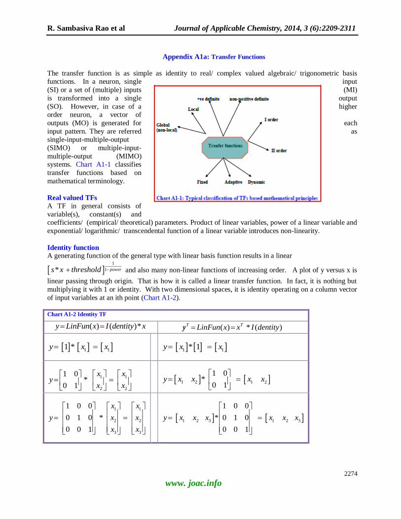
R. Sambasiva Rao et al Journal of Applicable Chemistry, 2014, 3 (6):2209-2311
2274
www. joac.info
Appendix A1a: Transfer Functions
The transfer function is as simple as identity to real/ complex valued algebraic/ trigonometric basis functions. In a neuron, single input
(SI) or a set of (multiple) inputs (MI)
is transformed into a single output
(SO). However, in case of a higher order neuron, a vector of
outputs (MO) is generated for each
input pattern. They are referred as single-input-multiple-output
(SIMO) or multiple-input-
multiple-output (MIMO) systems. Chart A1-1 classifies
transfer functions based on
mathematical terminology.
Real valued TFs A TF in general consists of
variable(s), constant(s) and coefficients/ (empirical/ theoretical) parameters. Product of linear variables, power of a linear variable and
exponential/ logarithmic/ transcendental function of a linear variable introduces non-linearity.
Identity function A generating function of the general type with linear basis function results in a linear
1
1* powers x threshold and also many non-linear functions of increasing order. A plot of y versus x is
linear passing through origin. That is how it is called a linear transfer function. In fact, it is nothing but
multiplying it with 1 or identity. With two dimensional spaces, it is identity operating on a column vector
of input variables at an ith point (Chart A1-2).
Chart A1-2 Identity TF
( ) ( )*y LinFun x I dentity x ( ) * ( )T Ty LinFun x x I dentity
1 11 *y x x
1 1* 1y x x
1 1
2 2
1 0*
0 1
x xy
x x
1 2 1 2
1 0*
0 1y x x x x
1 1
2 2
3 3
1 0 0
0 1 0 *
0 0 1
x x
y x x
x x
1 2 3 1 2 3
1 0 0
* 0 1 0
0 0 1
y x x x x x x

R. Sambasiva Rao et al Journal of Applicable Chemistry, 2014, 3 (6):2209-2311
2275
www. joac.info
If input space is one dimensional steepness parameter (s) = 1 power = 0 threshold = 0
& & &
Then
1
1 0( ) 1* 0 1*y LinFun x x x x
Thus, the simplest TF is identity. A few other simple TFs in 1D-input space are '-I', reciprocal, square root,
power operator etc.
Stuck function
A function outputting the same value (a constant, zero or one) is called a stuck function and practically
serves no purpose expect that it is an obstacle. The erroneous logic in software (Table A1-1) or malfunction in hardware/electronic devices is the reason behind it.
A numerical example with 'and' and 'or' relational operators are used to produce an output of one
and zero respectively, irrespective of the input is negative, positive integer/floating point value or even zero. A real number is +ve, -ve or zero only. The antecedent is always satisfied irrespective of the
condition and thus, output is stuck at 1. The 'and' clause is never be true and thus the output is always
zero. If there is no input to a system, obviously, there is no output. In other words, it is like absolute
silence.
Table A1-1 Stuck functions
Stuck at
Ex
Input output
1
Unconditional assignment y=1 -111 1
Antecedent never
saatisfied for a numeric value
and function [y] = om_stuck1and(x)
if x ==0 & x < 0 & x >0 y=0; else y = 1; end
0 1
or function [y] = om_stuck1(x) if x ==0 | x < 0 | x >0
y = 1; else y = 0; end
99 1
0
Unconditional assignment function [y] = om_stuck0(x) y=0;
-111 0
Antesedent is saatisfied always for a numeric
value
or function [y] = om_stuckor0(x) if x ==0 | x < 0 | x >0 y = 0 else y = 1; end
0 0
Antesedent is saatisfied
always for a numeric value
or function [y] = om_stuckor1(x)
if x ==0 | x < 0 | x >0 y = 1; else y = 0; end
99 0

R. Sambasiva Rao et al Journal of Applicable Chemistry, 2014, 3 (6):2209-2311
2276
www. joac.info
Threshold/bias/offset function It uses algebraic relational operator ('<', '>=') to output two integer (binary/bipolar) values, multiple
discrete/continuous values. The two valued function is referred as Hardlimitor
Symmetric Hardlimitor: The mathematical form of hardlimitor is depicted in Table A1-2. A matlab program (m file) implementing the expression as it is using a ‘ For‘ loop and if-then-else rule is given. A
concise form in tensor notation is also presented. Hardlimitor: The response is zero or one. It is used in electronics, classification to decipher whether it belongs to a
category or not.
Table A1-2: TF.Hardlimitor
Hardlimitor 0, 0
1
If x y
else y
x bi bip ---------------
-3 0 -1 -2 0 -1 -1 0 -1 0 1 1 1 1 1 2 1 1 3 1 1
Bipolar 0, 1
1
If x y
else y
%
% om_hardlimitor_binary.m (R S Rao 6/11/09, 5/4/99) % function [y_hardlimitor_binary, y_hardlimitor_bipolar, df,Name] = om_hardlimitor(x,fig) if nargin == 0 clean x = xgrid(-3,4,1);fig = 1;
end y_hardlimitor_binary = (x >= 0) ; y_hardlimitor_bipolar = 2*(x >= 0)-1 ;
-4 -2 0 2 40
0.2
0.4
0.6
0.8
1
-4 -2 0 2 4-1
-0.5
0
0.5
1
0.2
0.4
0.6
0.8
10 20 30 40
10
20
30
40
x1 (a)
x2
Fig.
0.1
0.2
0.3
0.4
0.5
0.6
0.70.80.9
-50
5
-50
50
0.5
1
(b)
-4 -2 0 2 40
0.2
0.4
0.6
0.8
1
Resp
x1 (c)-4 -2 0 2 40
0.2
0.4
0.6
0.8
1
Resp
x2 (d)
Step function: The step- and multiple step functions which are used as TFs in NNs are summarized in table A1-3.
Table A1-3: TF.Step function
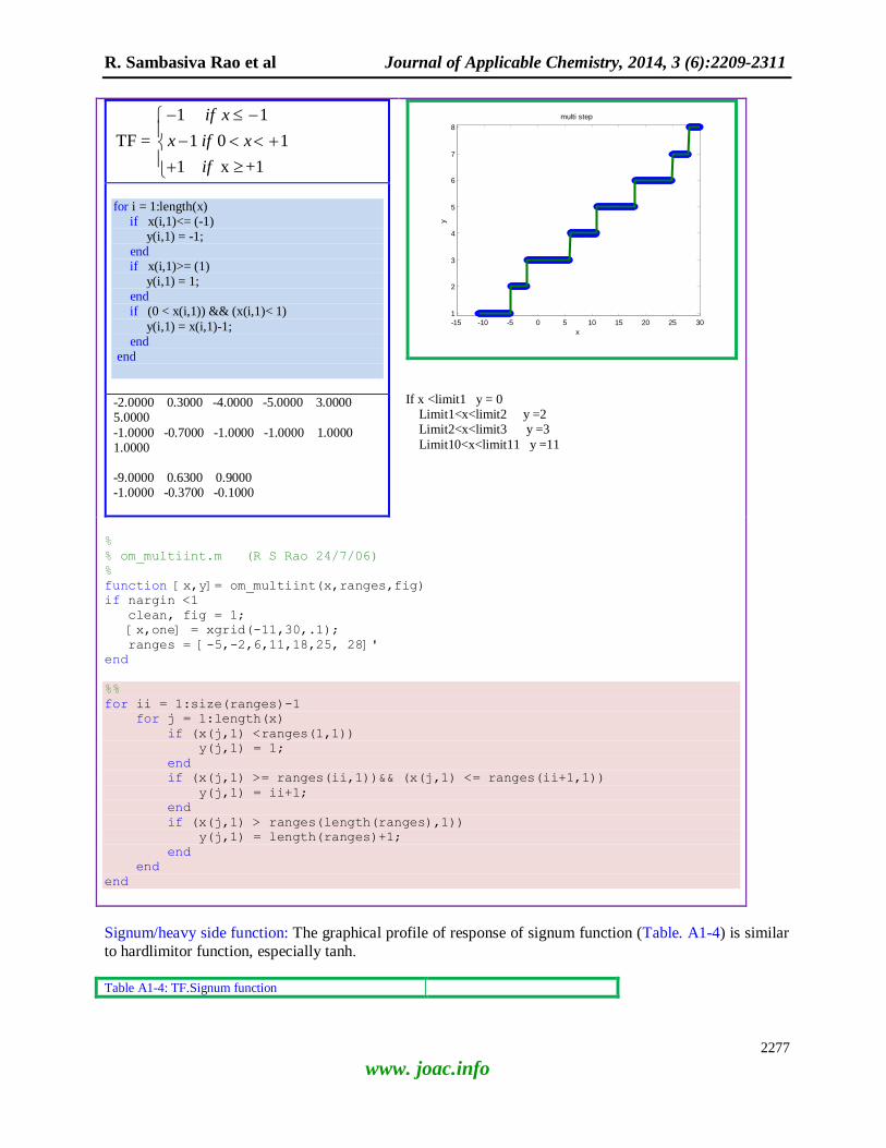
R. Sambasiva Rao et al Journal of Applicable Chemistry, 2014, 3 (6):2209-2311
2277
www. joac.info
1 1
TF = 1 0 1
1 x +1
if x
x if x
if
for i = 1:length(x) if x(i,1)<= (-1) y(i,1) = -1; end if x(i,1)>= (1) y(i,1) = 1; end if (0 < x(i,1)) && (x(i,1)< 1)
y(i,1) = x(i,1)-1; end end
-2.0000 0.3000 -4.0000 -5.0000 3.0000 5.0000
-1.0000 -0.7000 -1.0000 -1.0000 1.0000 1.0000 -9.0000 0.6300 0.9000 -1.0000 -0.3700 -0.1000
If x <limit1 y = 0 Limit1<x<limit2 y =2 Limit2<x<limit3 y =3
Limit10<x<limit11 y =11
%
% om_multiint.m (R S Rao 24/7/06)
%
function [x,y]= om_multiint(x,ranges,fig)
if nargin <1
clean, fig = 1;
[x,one] = xgrid(-11,30,.1);
ranges = [-5,-2,6,11,18,25, 28]'
end
%%
for ii = 1:size(ranges)-1
for j = 1:length(x)
if (x(j,1) <ranges(1,1))
y(j,1) = 1;
end
if (x(j,1) >= ranges(ii,1))&& (x(j,1) <= ranges(ii+1,1))
y(j,1) = ii+1;
end
if (x(j,1) > ranges(length(ranges),1))
y(j,1) = length(ranges)+1;
end
end
end
Signum/heavy side function: The graphical profile of response of signum function (Table. A1-4) is similar
to hardlimitor function, especially tanh.
Table A1-4: TF.Signum function
-15 -10 -5 0 5 10 15 20 25 30
1
2
3
4
5
6
7
8
multi step
x
y

R. Sambasiva Rao et al Journal of Applicable Chemistry, 2014, 3 (6):2209-2311
2278
www. joac.info
0
( ) 1
0
( ) 0
( ) 1
If x
then sign x
elseif x
sign x
else sign x
endif
y = sign(x);
Rectangular basis function: The output is a binary value depending upon whether the input is within or
outside a real interval (a to b) (Table A1-5).
Table A1-5: TF. Rectangular basisfunction
1tan ( )
0
if a x brec ular x
else
%
% om_rectangular.m (R S Rao 24/7/06)
%
function [rectangular]= om_rectangular(x,a,b,fig)
for i = 1:length(x)
if (le(a,x(i,1)) && x(i,1)<=b)
rectangular(i,1) = 1;
else
rectangular(i,1) = 0;
end
end
Linear generating function
Typical Linear functions include pure linear, linear_saturated, linear_saturated _symmetric ones. The profiles are straight lines and planes in 2D- input spaces (Table A1-6, Fig. A1-2). The input neurons of a
layered NN always have an identity TF, but popularly referred as linear one. In fact, in SLP_NN,
-6 -4 -2 0 2 4 6
-1
-0.8
-0.6
-0.4
-0.2
0
0.2
0.4
0.6
0.8
1
Signum Fn
x
y
-4 -3 -2 -1 0 1 2 3 4-0.5
0
0.5
1
1.5Rectangular TF
x
y

R. Sambasiva Rao et al Journal of Applicable Chemistry, 2014, 3 (6):2209-2311
2279
www. joac.info
MLP_NN, ART_NN, the input layer simply transmits the values as they are. In other words, the output of the input neuron is same as the input signal. In the case of function approximation problems, the output
neuron also has the same role. For classification tasks, the hard limiter TF is used to produce a binary
discrete classification label.
Table A1-6: TF.Linear functions
Linear $$$ Formula
Intelligent expression#
MATLAB code
Pure 1 0
TF = 1 0 1
1 x +1
if x
x if x
if
max(0,min(1,x))
linpure = x;
Positive
0TF =
0 0
x if x
if x
max(0,x)
linpos = max(0,x);
Saturating
Linsat =
max(0,min(1,x));
Saturating
symmetric
1 1
TF = 1 1
1 x +1
if x
x if x
if
max(-
1,min(1,x))
Linsatsym =
max(-1,min(1,x));
#:NMATLAB manual
Fig. A1-2: x-y plots, 3D-surfaces and 2D-contours for linear TF functions
linpure
-4 -3 -2 -1 0 1 2 3 4-4
-3
-2
-1
0
1
2
3
4
-5
0
5
10 20 30 40
10
20
30
40
x1 (a)
x2
Fig.
-6-4
-2
-2
0
0
2
2
46
-50
5
-50
5-10
0
10
(b)
-4 -2 0 2 4-10
-5
0
5
10
Resp
x1 (c)-4 -2 0 2 4
-10
-5
0
5
10
Resp
x2 (d)
Linpos

R. Sambasiva Rao et al Journal of Applicable Chemistry, 2014, 3 (6):2209-2311
2280
www. joac.info
-4 -3 -2 -1 0 1 2 3 40
0.5
1
1.5
2
2.5
3
3.5
4
0
1
2
3
10 20 30 40
10
20
30
40
x1 (a)
x2
Fig.
0.5
0.5
1
1
1.5
1.5
2
2
2.5
2.5
3
3
3.5
3.5
-50
5
-50
50
2
4
(b)
-4 -2 0 2 40
1
2
3
4
Resp
x1 (c)-4 -2 0 2 40
1
2
3
4
Resp
x2 (d)
linsat
-4 -3 -2 -1 0 1 2 3 40
0.1
0.2
0.3
0.4
0.5
0.6
0.7
0.8
0.9
1
0.2
0.4
0.6
0.8
10 20 30 40
10
20
30
40
x1 (a)
x2
Fig.
0.10.20.30.40.50.6
0.7
0.8
0.9
-50
5
-50
50
0.5
1
(b)
-4 -2 0 2 40
0.2
0.4
0.6
0.8
1R
esp
x1 (c)-4 -2 0 2 40
0.2
0.4
0.6
0.8
1
Resp
x2 (d) linsatsym
-4 -3 -2 -1 0 1 2 3 4-1
-0.8
-0.6
-0.4
-0.2
0
0.2
0.4
0.6
0.8
1
-1
-0.5
0
0.5
10 20 30 40
10
20
30
40
x1 (a)
x2
Fig.
-0.8
-0.8
-0.6
-0.6
-0.4
-0.4-0.2
0
0
0.2
0.4
0.6
0.8
-5
0
5
-5
0
5-1
0
1
(b)
-4 -2 0 2 4-1
-0.5
0
0.5
1
Resp
x1 (c)
-4 -2 0 2 4-1
-0.5
0
0.5
1
Resp
x2 (d)
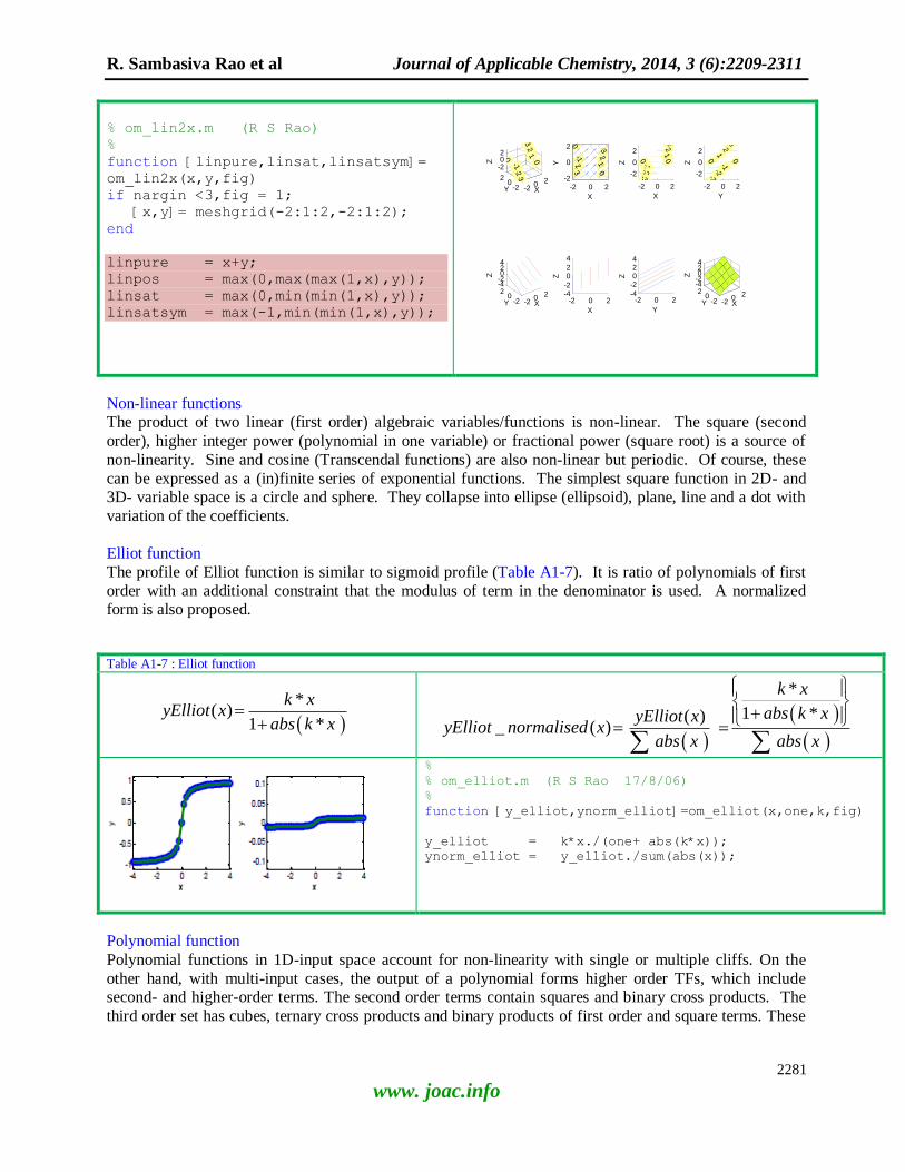
R. Sambasiva Rao et al Journal of Applicable Chemistry, 2014, 3 (6):2209-2311
2281
www. joac.info
% om_lin2x.m (R S Rao)
%
function [linpure,linsat,linsatsym]=
om_lin2x(x,y,fig)
if nargin <3,fig = 1;
[x,y]= meshgrid(-2:1:2,-2:1:2);
end
linpure = x+y;
linpos = max(0,max(max(1,x),y));
linsat = max(0,min(min(1,x),y));
linsatsym = max(-1,min(min(1,x),y));
Non-linear functions The product of two linear (first order) algebraic variables/functions is non-linear. The square (second
order), higher integer power (polynomial in one variable) or fractional power (square root) is a source of
non-linearity. Sine and cosine (Transcendal functions) are also non-linear but periodic. Of course, these
can be expressed as a (in)finite series of exponential functions. The simplest square function in 2D- and 3D- variable space is a circle and sphere. They collapse into ellipse (ellipsoid), plane, line and a dot with
variation of the coefficients.
Elliot function
The profile of Elliot function is similar to sigmoid profile (Table A1-7). It is ratio of polynomials of first
order with an additional constraint that the modulus of term in the denominator is used. A normalized form is also proposed.
Table A1-7 : Elliot function
*
( )1 *
k xyElliot x
abs k x
*
1 *( )_ ( )
k x
abs k xyElliot xyElliot normalised x
abs x abs x
%
% om_elliot.m (R S Rao 17/8/06)
%
function [y_elliot,ynorm_elliot]=om_elliot(x,one,k,fig)
y_elliot = k*x./(one+ abs(k*x));
ynorm_elliot = y_elliot./sum(abs(x));
Polynomial function
Polynomial functions in 1D-input space account for non-linearity with single or multiple cliffs. On the
other hand, with multi-input cases, the output of a polynomial forms higher order TFs, which include second- and higher-order terms. The second order terms contain squares and binary cross products. The
third order set has cubes, ternary cross products and binary products of first order and square terms. These
-20 2
-20
2
-202
-3-2
-1
00
12
Z
3
XY
-3-2
-1
0
0
12
3
X
Y
-2 0 2-2
0
2
-2 0 2
-2
0
2
32
100
Z -1-2
-3
X
-2 0 2
-2
0
2
32
10 0
Z -1-2
-3Y
-20 2
-20
2-4-2024
XY
Z
-20 2
-20
2-4-2024
XY
Z
-2 0 2-4-2
02
4
X
Z
-2 0 2-4
-2024
Y
Z

R. Sambasiva Rao et al Journal of Applicable Chemistry, 2014, 3 (6):2209-2311
2282
www. joac.info
higher order functions and Clifford geometric entities are the prospecting TFs of this decade. There are still only scanty reports in many application fields.
Exponential function Softmax is normallized exponential
function. The combination of
simplest exponential functions viz.
exp(x) and exp(-x) generate sinh, cosh, and the sought after tanh. The
range of tanh is -1 to +1, producing a
symmetric profile around zero. The popular RBF is also an exponential
function with (-x2) as an argument. The range of output is 0 to 1 as x moves from to (Table A1-9a).
The bipolar output is readily transformable into bipolar sigmoid.
Softmax function (table A1-8)
The range of softmax is 0 to 1.
Sigmoid function
It is a non-decreasing or monotonously increasing smooth function bounded between real values of 0 and
1. Analytical derivatives (gradient and Hessian) exist (chart A1-3). The universal function approximation
theorem was proved for MLP_NN with sigmoid TF, the consequence being any non-linear function can be approximated for any desired accuracy. The formulae and object module (om) of matlab functions are
given in table A1-9. Sigmoid TF produces linearly independent internal representation [23].
Sigmoid on hardware
Armato et al. [254] proposed calculation of low-error approximation of sigmoid and subsequently
hyperbolic tangent (tanh) function using piece wise linear procedure. The minimum number of precision bits for convergence for MLP_NN is arrived. This approach resulted in smaller absolute as well as mean
relative errors compared to state-of-art-methods. The digital implementation of sigmoid function has
favorable score in terms of lower complexity and error. Sigmoid and tanh are used in TFs in artificial
neurons. Thus, it plays a crucial role in hardware implementation of mathematical neurons (man). VHDL approximation of Taylor series of sigmoid is with an error of 0.005 in the entire range (Chart A1-4).
Another method using CORDIC algorithm calculates hyperbolic sine and cosine functions. Tanh
calculated as the ratio of sinh to cosh is used to obtain sigmoid. Two segments (0 to 2 and 2 to 4) are used. When an accurate result is desired more CORDIC rotations are used. The error in this method also
remains around 0.005.
Chart A1-4: Hardware computation of sigmoid function
x SG(x)
Tanh(x) g(TF)
SG Tanh
If x 0 -1 0 0
If x 1 1 0 0
If x 0 0 0 -- ---
TF_SG
- Shape restriction of profile
Remedy : Higher order TF
m-SG Generalized RBF
Expert opinions –
(use with caution)
If TF is bipolar sigmoid function (tanh) [ -1 to +1] Then convergence speed increases
Table A1-8 : Softmax function
exp( )max
exp( )
xysoft
x
% % om_softmax.m (R S Rao 5/4/99) % function [ysoftmax,Name]= om_softmax(x,one) expn = exp(x);
ysoftmax = expn./ sum(expn,1); Name = ‗TF_SoftMax‘;

R. Sambasiva Rao et al Journal of Applicable Chemistry, 2014, 3 (6):2209-2311
2283
www. joac.info
If K,D, L paramters are also refined along with W in BP
Then NN approximates a nonlin function more closely
Chart A1-3 : Sigmoid function and its first (gradient) and second (Hessian) derivatives
TF = ( )
(TF) = =d TF
gdx
2
2
(g( )) ( )(TF) = = =
d TF d TFH
dx dx
1
( )1 exp * 4
SG xx s b
s*SG * (1-SG) 2s *SG * (1-SG) *(2-SG)
1 exptanh( )
1 exp
xx
x
1 tanh * 1 tanh
2
tanh* 1 tanh * 1 tanh
2
par_SG : [s,threshold] ; ySG = SG(x;par_SG) = SG(x)
Table A1-9a: sigmoid TF
% % om_sg.m (R S Rao 5/4/99) % function [sg,dsg,d2sg,name] = om_sg(x,s,threshold,one) sg = one./(one + exp(-x*s + threshold *one)); dsg = sg.* (one-sg); d2sg = sg.* (one-sg).* (one - 2*sg);
name = 'Sigmoid';
% % om_tanh.m (R S Rao 8/8/10, 5/4/99) % function [tanhx,dtanhx] = om_tanh(x,one,t) tanhx = (exp(x/t) - exp(-x/t))./(exp(x/t)+ exp(-x/t)); dtanhx = (one+tanhx).*(one-tanhx)/2;
The multiplication two vectors by the rules of extended matrix notation ( i.e. element wise multiplication)
is used (table A1-9b).
Table A1-9b: Sigmoid function in two dimensions
-4 -2 0 2 4
0
0.5
1
x
y
-4 -2 0 2 4
-1
-0.5
0
0.5
1
sigmoid(x) tanh(x)
x
y

R. Sambasiva Rao et al Journal of Applicable Chemistry, 2014, 3 (6):2209-2311
2284
www. joac.info
%
% dem_sg2x.m 18/10/03 (12:00 hrs)
%
function [sg2sum] = om_sg2xT(xx,yy,steep,threshold,fig)
if nargin<4, clean,fig = 1;
[xx,yy]= meshgrid(-3:0.5:3,-3:0.5:3);
threshold = 0;steep = 1e4,A = 1;
end
[r,c]= size(xx); one = ones(r,c);
[sg1,dsg,d2sg,name] = om_sg(xx,steep,threshold,one); % Table A1-9a (om_sg.m) [sg2,dsg,d2sg,name] = om_sg(yy,steep,threshold,one);
surf(xx,yy, sg1.*sg2)
By changing the threshold and steepness parameters, sigmoid emulates hard limiter, linear functions etc.
(table A1-10).
Table A1-10: sigmoid function emulating hardlimitor, straight line
-4
-2
0
2
4
-4
-2
0
2
40
0.2
0.4
0.6
0.8
1

R. Sambasiva Rao et al Journal of Applicable Chemistry, 2014, 3 (6):2209-2311
2285
www. joac.info
Threshold: [ 1e-4 1 -1 -100 100]'
Slope = 1
Steepness : [1e-4 1 -1 -1e2 1e2]
Threshold = 0
%
% dem_sgk.m (R S Rao 12/05/05 ; R Naga Satish 30/07/2001)
%
clean
[x] = [-4:.1:4]';
[r,c]=size(x); one = ones(r,c);
format short g
%
% Threshold
%
k = 1;
thz = [ 1e-4 1 -1 -1e2 1e2 ]';
[rth,cth]=size(thz);
for i = 1:rth
th = thz(i,1);
[t2] = om_sg(x,k,th,one);
T3(:,i)= t2;
end
plot2d(x,T3)
plot2d(x,T3(:,1),T3(:,2),T3(:,3),T3(:,4),T3(:,5))
%
% steepness
%
kz = [ 1e-4 1 -1 -1e2 1e2 ]';
[rk,ck]=size(kz);
for i = 1:rk
k = kz(i,1);
[t2] = om_sg(x,k,0,one);
T4(:,i)= t2;
end
plot2d(x,T4)
plot2d(x,T4(:,1),T4(:,2),T4(:,3),T4(:,4),T4(:,5))
Table A1-11 shows the effect of variation of power in extended-sigmoid function profiles.
Table A1-11: Effect of power parameter on sigmoid function profiles
-4 -3 -2 -1 0 1 2 3 4
0
0.2
0.4
0.6
0.8
1
Treshold variation
x
y
-4 -3 -2 -1 0 1 2 3 4
0
0.2
0.4
0.6
0.8
1
steepness variation
x
y
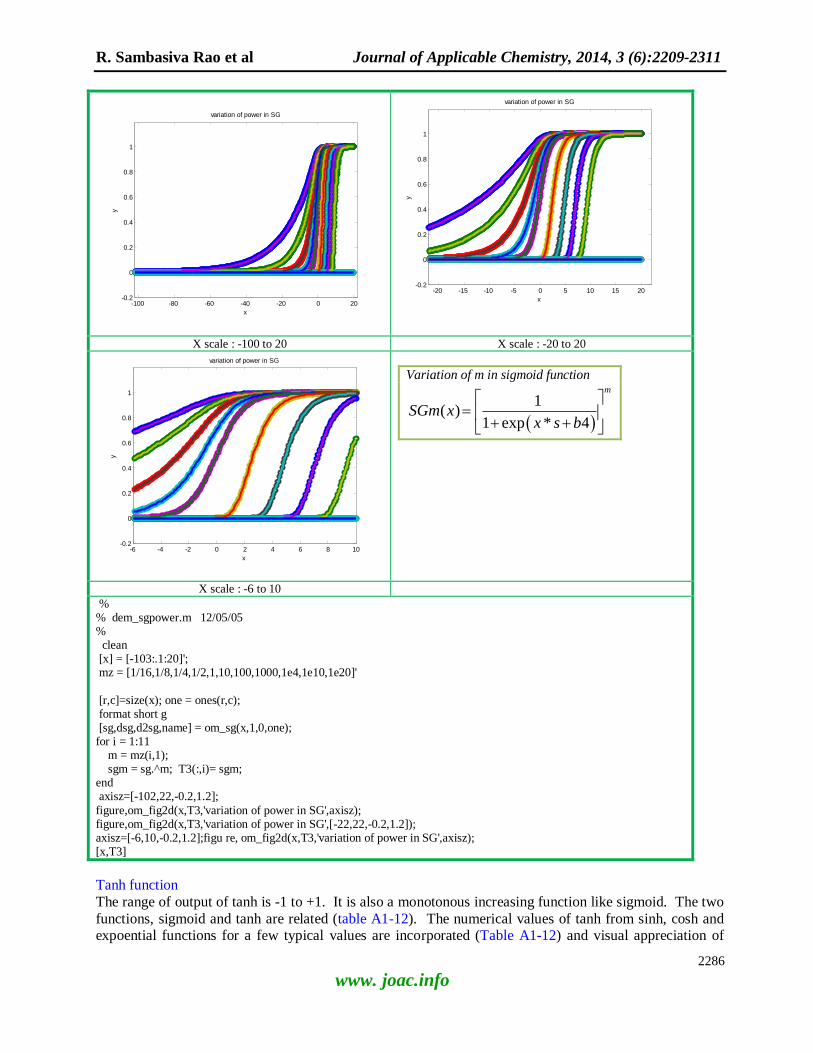
R. Sambasiva Rao et al Journal of Applicable Chemistry, 2014, 3 (6):2209-2311
2286
www. joac.info
X scale : -100 to 20 X scale : -20 to 20
Variation of m in sigmoid function
1
( )1 exp * 4
m
SGm xx s b
X scale : -6 to 10
% % dem_sgpower.m 12/05/05 % clean [x] = [-103:.1:20]'; mz = [1/16,1/8,1/4,1/2,1,10,100,1000,1e4,1e10,1e20]'
[r,c]=size(x); one = ones(r,c); format short g [sg,dsg,d2sg,name] = om_sg(x,1,0,one); for i = 1:11 m = mz(i,1); sgm = sg.^m; T3(:,i)= sgm; end axisz=[-102,22,-0.2,1.2];
figure,om_fig2d(x,T3,'variation of power in SG',axisz); figure,om_fig2d(x,T3,'variation of power in SG',[-22,22,-0.2,1.2]); axisz=[-6,10,-0.2,1.2];figu re, om_fig2d(x,T3,'variation of power in SG',axisz); [x,T3]
Tanh function
The range of output of tanh is -1 to +1. It is also a monotonous increasing function like sigmoid. The two
functions, sigmoid and tanh are related (table A1-12). The numerical values of tanh from sinh, cosh and expoential functions for a few typical values are incorporated (Table A1-12) and visual appreciation of
-100 -80 -60 -40 -20 0 20-0.2
0
0.2
0.4
0.6
0.8
1
variation of power in SG
x
y
-20 -15 -10 -5 0 5 10 15 20-0.2
0
0.2
0.4
0.6
0.8
1
variation of power in SG
x
y
-6 -4 -2 0 2 4 6 8 10-0.2
0
0.2
0.4
0.6
0.8
1
variation of power in SG
x
y
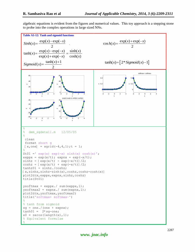
R. Sambasiva Rao et al Journal of Applicable Chemistry, 2014, 3 (6):2209-2311
2287
www. joac.info
algebraic equations is evident from the figures and numerical values. This toy approach is a stepping stone to probe into the complex operations in large sized NNs.
Table A1-12: Tanh and sigmoid functions
exp( ) exp( )( )
2
x xSinh x
.
exp( ) exp( )cos ( )
2
x xh x
exp( ) exp( ) sinh( )tanh( )
exp( ) exp( ) cosh( )
x x xx
x x x
tanh( ) 1( )
2
xSigmoid x
tanh( ) 2* ( ) 1x Sigmoid x
%
% dem_sgdetail.m 12/05/05
%
clean
format short g
[x,one] = xgrid(-4,4,1);t = 1;
%
St01 =' exp(x) exp(-x) sinh(x) cosh(x)';
exppx = exp(x/t); expnx = exp(-x/t);
sinhz = [exp(x/t) - exp(-x/t)]/2;
coshz = [exp(x/t) + exp(-x/t)]/2;
tanhz01 = sinhz./coshz;
[x,sinhz,sinhz-sinh(x),coshz,coshz-cosh(x)]
plot2d(x,exppx,expnx,sinhz,coshz)
title(St01)
ysoftmax = exppx./ sum(exppx,1);
ysoftmax2 = expnx./ sum(expnx,1);
plot2d(x,ysoftmax,ysoftmax2)
title('softmax+ softmax-')
%
% tanh from sigmoid
sg = one./(one + expnx);
tanh01 = 2*sg-one;
x0 = zeros(length(x),1);
% Equivalent formulae
%
-4 -2 0 2 40
20
40
60
x
y
-4 -2 0 2 40
20
40
60
x
y
-4 -2 0 2 4-40
-20
0
20
40
x
y
-4 -2 0 2 40
10
20
30 exp(x) exp(-x) sinh(x) cosh(x)
x
y
-4 -2 0 2 4
0
0.2
0.4
x
y
-4 -2 0 2 4
0
0.2
0.4
softmax+ softmax-
x
y
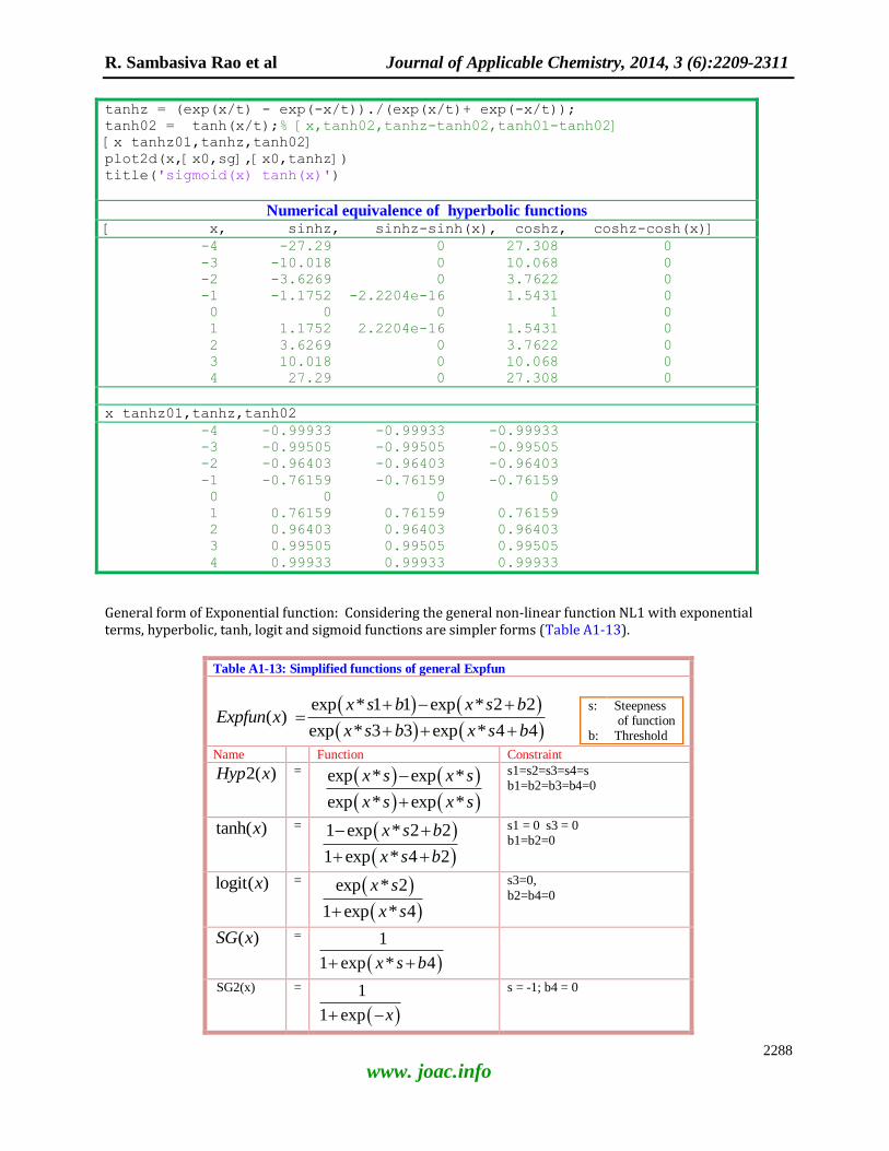
R. Sambasiva Rao et al Journal of Applicable Chemistry, 2014, 3 (6):2209-2311
2288
www. joac.info
tanhz = (exp(x/t) - exp(-x/t))./(exp(x/t)+ exp(-x/t));
tanh02 = tanh(x/t);% [x,tanh02,tanhz-tanh02,tanh01-tanh02]
[x tanhz01,tanhz,tanh02]
plot2d(x,[x0,sg],[x0,tanhz])
title('sigmoid(x) tanh(x)')
Numerical equivalence of hyperbolic functions [ x, sinhz, sinhz-sinh(x), coshz, coshz-cosh(x)]
-4 -27.29 0 27.308 0
-3 -10.018 0 10.068 0
-2 -3.6269 0 3.7622 0
-1 -1.1752 -2.2204e-16 1.5431 0
0 0 0 1 0
1 1.1752 2.2204e-16 1.5431 0
2 3.6269 0 3.7622 0
3 10.018 0 10.068 0
4 27.29 0 27.308 0
x tanhz01,tanhz,tanh02
-4 -0.99933 -0.99933 -0.99933
-3 -0.99505 -0.99505 -0.99505
-2 -0.96403 -0.96403 -0.96403
-1 -0.76159 -0.76159 -0.76159
0 0 0 0
1 0.76159 0.76159 0.76159
2 0.96403 0.96403 0.96403
3 0.99505 0.99505 0.99505
4 0.99933 0.99933 0.99933
General form of Exponential function: Considering the general non-linear function NL1 with exponential terms, hyperbolic, tanh, logit and sigmoid functions are simpler forms (Table A1-13).
Table A1-13: Simplified functions of general Expfun
exp * 1 1 exp * 2 2( )
exp * 3 3 exp * 4 4
x s b x s bExpfun x
x s b x s b
s: Steepness of function
b: Threshold
Name Function Constraint
2( )Hyp x =
exp * exp *
exp * exp *
x s x s
x s x s
s1=s2=s3=s4=s b1=b2=b3=b4=0
tanh( )x =
1 exp * 2 2
1 exp * 4 2
x s b
x s b
s1 = 0 s3 = 0 b1=b2=0
logit( )x =
exp * 2
1 exp * 4
x s
x s
s3=0,
b2=b4=0
( )SG x =
1
1 exp * 4x s b
SG2(x) =
1
1 exp x
s = -1; b4 = 0
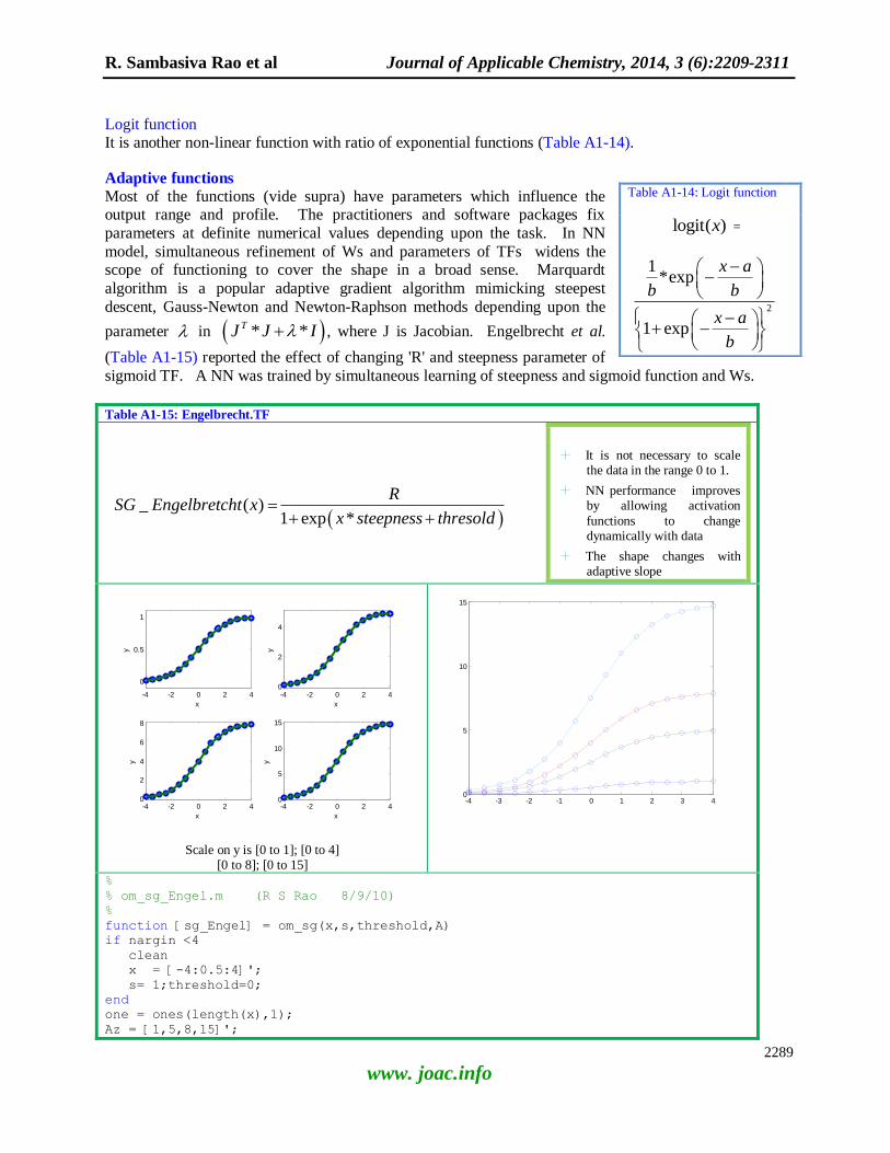
R. Sambasiva Rao et al Journal of Applicable Chemistry, 2014, 3 (6):2209-2311
2289
www. joac.info
Logit function It is another non-linear function with ratio of exponential functions (Table A1-14).
Adaptive functions
Most of the functions (vide supra) have parameters which influence the output range and profile. The practitioners and software packages fix
parameters at definite numerical values depending upon the task. In NN
model, simultaneous refinement of Ws and parameters of TFs widens the scope of functioning to cover the shape in a broad sense. Marquardt
algorithm is a popular adaptive gradient algorithm mimicking steepest
descent, Gauss-Newton and Newton-Raphson methods depending upon the
parameter in * *TJ J I , where J is Jacobian. Engelbrecht et al.
(Table A1-15) reported the effect of changing 'R' and steepness parameter of
sigmoid TF. A NN was trained by simultaneous learning of steepness and sigmoid function and Ws.
Table A1-15: Engelbrecht.TF
_ ( )
1 exp *
RSG Engelbretcht x
x steepness thresold
It is not necessary to scale the data in the range 0 to 1.
NN performance improves by allowing activation
functions to change dynamically with data
The shape changes with adaptive slope
Scale on y is [0 to 1]; [0 to 4]
[0 to 8]; [0 to 15]
%
% om_sg_Engel.m (R S Rao 8/9/10)
%
function [sg_Engel] = om_sg(x,s,threshold,A)
if nargin <4
clean
x = [-4:0.5:4]';
s= 1;threshold=0;
end
one = ones(length(x),1);
Az = [1,5,8,15]';
Table A1-14: Logit function
logit( )x =
2
1*exp
1 exp
x a
b b
x a
b
-4 -2 0 2 4
0
0.5
1
x
y
-4 -2 0 2 40
2
4
x
y
-4 -2 0 2 40
2
4
6
8
x
y
-4 -2 0 2 40
5
10
15
x
y
-4 -3 -2 -1 0 1 2 3 40
5
10
15

R. Sambasiva Rao et al Journal of Applicable Chemistry, 2014, 3 (6):2209-2311
2290
www. joac.info
for i = 1:length(Az)
A = Az(i,1);
sg_Engel(:,i) = (A*one)./(one + exp(-x*s + threshold *one));
end
[x,sg_Engel]
plot2d(x,sg_Engel(:,1), sg_Engel(:,2), sg_Engel(:,3), sg_Engel(:,4))
figure, plot (x,sg_Engel,x,sg_Engel,'bo')
Wavelet function Wavelet functions played a typical role as TFs to model filtering tasks, which are not easily modeled by
local exponential and polynomial functions. Table A1-16 describes x-y plot and 3D-surface for a two variable
triangular functions.
Table A1-16: Triangular.TF
% % om_triangular.m (R S Rao 7/7/06, 5/4/99) % function [f] = om_trianular(x,y,fig) % if nargin <1
-4
-2
0
2
4
-4
-2
0
2
40
1
2
3
4
5
-4 -3 -2 -1 0 1 2 3 4
0
0.2
0.4
0.6
0.8
1
x
y
-202 4
-2024
2
4
0.511.522.5
333.
5
3.54
4
Z
4.5 4.5
XY
0.511.522.5
3
3
3.5
3.5
4
4
4.5
4.5
5
5
X
Y
-4 -2 0 2 4-5
0
5
-4 -2 0 2 4
2
4
4.5 4.54 4
3.5 3.53
32.5Z
21.5
10.5
X
-4 -2 0 2 4
2
4
4.54.5 4
4 3.53.5 3
32.5Z
21.5
10.5
Y
-4-2024
-4-20240
5
XY
Z
-4-2024
-4-20240
5
XY
Z
-4 -2 0 2 40
5
X
Z
-4 -2 0 2 40
5
Y
Z
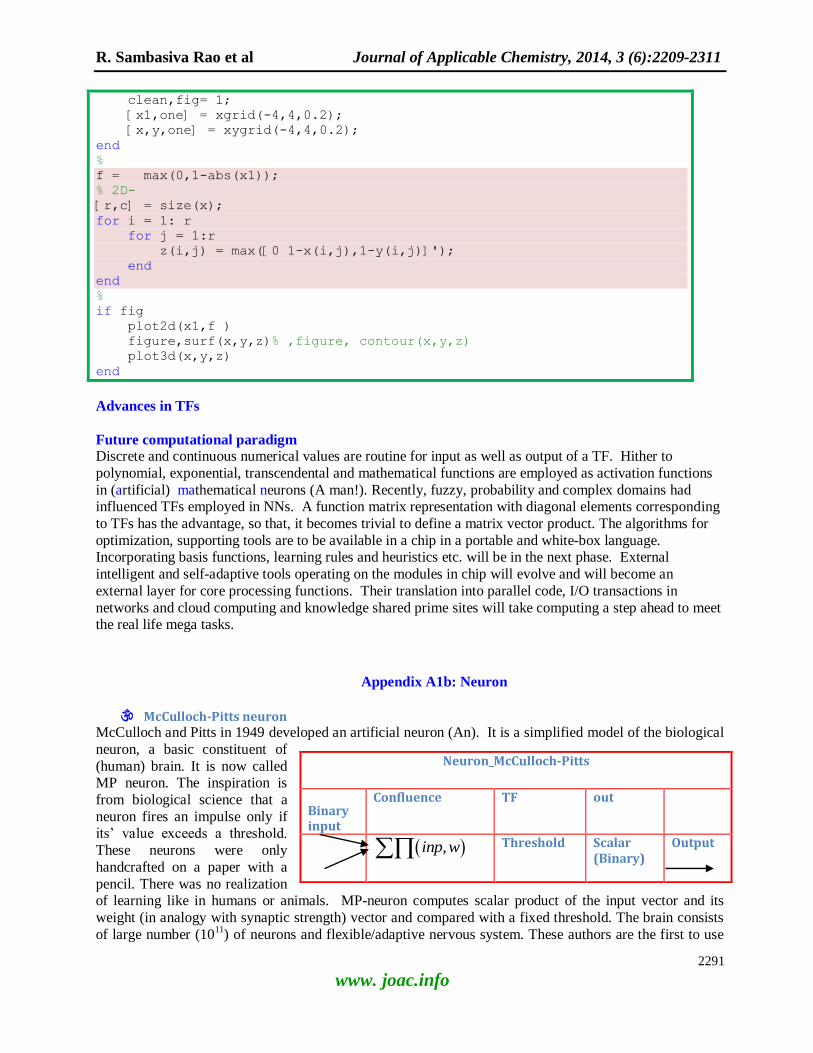
R. Sambasiva Rao et al Journal of Applicable Chemistry, 2014, 3 (6):2209-2311
2291
www. joac.info
clean,fig= 1; [x1,one] = xgrid(-4,4,0.2); [x,y,one] = xygrid(-4,4,0.2); end % f = max(0,1-abs(x1)); % 2D- [r,c] = size(x); for i = 1: r for j = 1:r z(i,j) = max([0 1-x(i,j),1-y(i,j)]'); end end % if fig plot2d(x1,f ) figure,surf(x,y,z)% ,figure, contour(x,y,z) plot3d(x,y,z) end
Advances in TFs
Future computational paradigm Discrete and continuous numerical values are routine for input as well as output of a TF. Hither to
polynomial, exponential, transcendental and mathematical functions are employed as activation functions
in (artificial) mathematical neurons (A man!). Recently, fuzzy, probability and complex domains had influenced TFs employed in NNs. A function matrix representation with diagonal elements corresponding
to TFs has the advantage, so that, it becomes trivial to define a matrix vector product. The algorithms for
optimization, supporting tools are to be available in a chip in a portable and white-box language. Incorporating basis functions, learning rules and heuristics etc. will be in the next phase. External
intelligent and self-adaptive tools operating on the modules in chip will evolve and will become an
external layer for core processing functions. Their translation into parallel code, I/O transactions in
networks and cloud computing and knowledge shared prime sites will take computing a step ahead to meet the real life mega tasks.
Appendix A1b: Neuron
McCulloch-Pitts neuron McCulloch and Pitts in 1949 developed an artificial neuron (An). It is a simplified model of the biological
neuron, a basic constituent of
(human) brain. It is now called MP neuron. The inspiration is
from biological science that a
neuron fires an impulse only if its‘ value exceeds a threshold.
These neurons were only
handcrafted on a paper with a
pencil. There was no realization of learning like in humans or animals. MP-neuron computes scalar product of the input vector and its
weight (in analogy with synaptic strength) vector and compared with a fixed threshold. The brain consists
of large number (1011
) of neurons and flexible/adaptive nervous system. These authors are the first to use
Neuron_McCulloch-Pitts
Binary input
Confluence TF out
,inp w Threshold Scalar
(Binary) Output

R. Sambasiva Rao et al Journal of Applicable Chemistry, 2014, 3 (6):2209-2311
2292
www. joac.info
the phrase 'Neural network'. Using these neurons, McCulloch and Pitts neural network explained Boolean gates ('AND', 'OR', 'NOT'). Table A1.17 details copying operation with this NN. But, MP-NN is too
simple a model to explain miraculous and sparkling endeavors of human brain in wakeup, sleep and dream
states, leave alone at mind and conscious levels.
Table A1-17 Copying operation with a neuron
Artificial neuron
Operation
of TF Result Example
Input Output
Input output
I(dentity) Copying 1 1
-1 1
-I Inversion 1 -1
-1 1
Formulae: one = unit column vector; inp = input vector to neuron; OI: output of input x = inpT*one;
OI = TF(x);
Ex 1: copying: inp = 1; TF = eye(1); one = [1]; x = inpT*one = [1]*[1] = 1; OI = TF(x) = I(x) = I(1) = 1;
Ex 2:Negation : inp = 1; TF = -I; x = inpT*one = [1]*[1] = 1; OI = TF(x) = -I(x) = -I(1) = -1;
McCulloch and Pitts neuron
First mathematical model of a biological neuron
Emulates binary 'and, or, not' gates
- Fixed threshold
- Fixed weights
- Hard-wired logic devices that were setup manually
- No ability to learn
Remedy : Hebb's learning rule
*Tynn TF X W
( )
* * *
*
T T T
T
If TF is linear Identity
ThenTF X W I X W X W
If threshold is included
Then ynn X W threshold
Outstar and instar type neurons
Stephen Grossberg used the analogy of inwardly radiating star to describe the connections between
neurons or a neuron and networks. If a neuron in the web (net) of other neurons receives a large number of
inputs, then it is termed as instar (Fig. A1-3a). Ideally, an instar neuron is not expected to have any
connections going out of it. The net input to an instar type neuron is XT * W. On the other hand, a neuron
sending many outputs to other destinations is called an outstar (Fig. A1-3b). A neuron of MISO in
input/output or hidden layer (SLP, MLP) is an 'instar' type. On the other hand, SIMO, 2IMO prevalent in
higher order neurons (Fig. A1-3e, f) are predominantly outstar. The neurons in the hidden layers, higher order neurons or those in robots are MIMO
category. Hecht-Nielson counter propagation
(CP) NN behaves both as instar and outstar.
Bias (Threshold) neuron The output of a bias neuron is always one.
Neuron_Bias
a0 Confl TF out output
0,a I I a0
TF(.)

R. Sambasiva Rao et al Journal of Applicable Chemistry, 2014, 3 (6):2209-2311
2293
www. joac.info
There is no input to this neuron. It can be deemed as NISO (No input single output) system with the output is stuck at one. It is used to include a constant (intercept) in a linear model. Threshold, so called
bias, can be understood as a weight coefficient of the connection formally added neuron j, where xj = 1
Modified neuron
The net signal i.e. weighted input calculated as the dot product (XT*W) is passed through a transfer (TF)
/activation function (AF) whereby capability of neuron in I/O mapping improves substantially. The TF can be as simple as identity, linear or non-linear.
Fig. A1-3: Classification of neuron based number of inputs and outputs
-neuron
The confluence operator in -neuron (sigma-neuron) is sum (Chart A1-5). MC-neuron, Rosenblatt neuron, sigmoid neurons are a few examples of it.
-neuron In this neuron, the confluence operator is a product of input element and corresponding weight.
Power-neuron In power neuron, the confluence operator is a product of input element raised to the power of corresponding weight.
Geometric mean neuron
It uses aggregation or accumulation function based on geometric mean of all inputs.

R. Sambasiva Rao et al Journal of Applicable Chemistry, 2014, 3 (6):2209-2311
2294
www. joac.info
Rosenblatt perceptron
Frank Rosenblatt invented perceptron at the Cornell Aeronautical Laboratory in 1957. The goal was an attempt to understand human memory, learning, and cognitive processes. In 1960 Rosenblatt demonstrated
the Mark I Perceptron. The Mark I was the first machine that could "learn" to identify optical patterns. He
proposed a learning neural network model, a significant improvement to McCulloch and Pitts (MP) neuron. Rosenblatt-neuron learns responses by refining weights. It is the start of successful machine
learning.
Chart A1-5: Neurons
-neuron
'*sum x w
Example
1
1 2 3 2
3
*
w
x x x w
w
1 1 2 2 3 3* * *x w x w x w
-neuron
.*prod x w
Example
11
* 2 * 2* *0.5*2 1 2 30.53 .
x
x x x x
x
power-neuron
.^prod x w
11^ 22
0.53 .
2* *1 2 3
x
x
x
x x x
Rosenblatt perceptron
Learns linearly separable Boolean gates o ('AND', 'OR', 'NOT')
Learns patterns (alphabets)
- Cannot model dynamic tasks
o Remedy : Dynamic neuron
- Unable to learn classification tasks
with quadratic/non-linear separation boundaries
XOR, which is not linearly separable
Remedy : Sigmoid neuron
Direct Parallel Perceptron A Gaussian kernel and a linear classifier (perceptron) are used [255].
Direct Kernel Perceptron (DKP)
Fernández-Delgado et al. [255] proposed direct kernel perceptron (DKP) with inspiration from direct
parallel perceptron. DKP is related to SVM and extreme learning machine. The image-coefficients are calculated by analytical closed-form expression directly and thus do not involve any iterative training. It
requires only training patterns. Further, this algorithm does not use any tunable regularization parameters.
Also, Ws are translatable to image-coefficient employing a variable change.

R. Sambasiva Rao et al Journal of Applicable Chemistry, 2014, 3 (6):2209-2311
2295
www. joac.info
Linear neuron
The biological inspiration is from Limulus-eye, cortical micro-circuits and firing rate in nerve cells. The
saturating behavior is due to absolute refractory period. The presence of a unique stationary point is the
sufficient condition and the output is confined to positive real axis.
Bernard Widrow (from electrical engineering at Stanford University) with his doctoral student Ted Hoff
proposed adoptive linear neuron in the year 1959. The activation/transfer function is a non-saturating one
and unbounded.
Sigmoid neuron
In 1986, Rumelhard used real valued sigmoid
function as TF in the neuron. It accepts multiple numerical inputs and generates a single scalar
output. The NN with these sigmoid neurons and
back-propagation learning successfully modeled XOR task, which remained unsolved for over three decades with linear NN paradigm. Later, different forms of sigmoid type exponential functions viz. tanh,
logarithm of sigmoid have become popular as TFs.
Advances in (artificial) neuron or processing unit RBF-, self organizing-, ART- and recurrent neurons are detailed in our earlier reviews [303-308].
Wavelet-neuron It is a neuron with (radial mother) wavelet as TF and also referred as wavelon. The dilation (Tj)
and translation (E) operators are used in the
Gaussian kernel.
i
jii
t
exFy
Rectangular wave neuron
A rectangular wave neuron has a transfer function of a certain real number with infinite intervals.
Neuron with more than one TF
Two transfer functions instead of only one are used over the last half a century. A linear combination of the outputs of the two TFs imparts more non-linearity.
_ max '* ,0TF linearThreshold x w threshold
Neuron_Lin
input Confl TF out output
,inp w sigmoid scalar
Neuron_Wavelet (wavelon)
input Confl TF out output
,inp w wavelet
Neuron_Rectang
input Confl TF out output
,inp w Rectangular
function
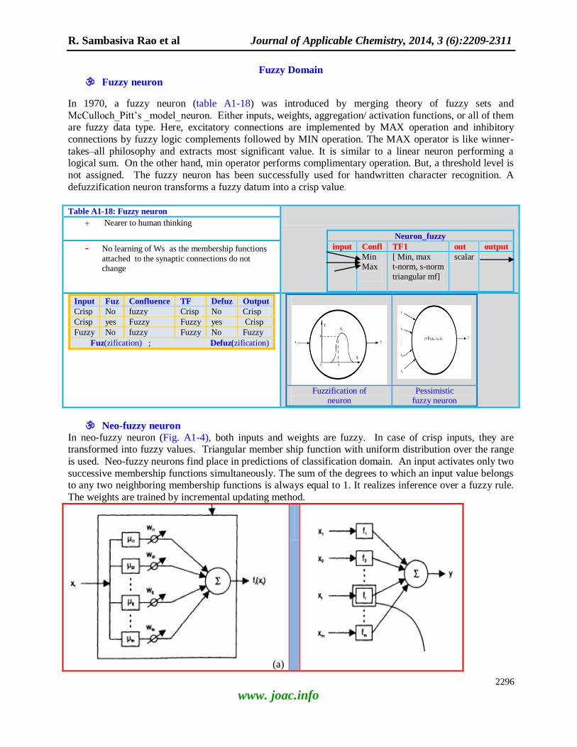
R. Sambasiva Rao et al Journal of Applicable Chemistry, 2014, 3 (6):2209-2311
2296
www. joac.info
Fuzzy Domain
Fuzzy neuron
In 1970, a fuzzy neuron (table A1-18) was introduced by merging theory of fuzzy sets and
McCulloch_Pitt‘s _model_neuron. Either inputs, weights, aggregation/ activation functions, or all of them are fuzzy data type. Here, excitatory connections are implemented by MAX operation and inhibitory
connections by fuzzy logic complements followed by MIN operation. The MAX operator is like winner-
takes–all philosophy and extracts most significant value. It is similar to a linear neuron performing a logical sum. On the other hand, min operator performs complimentary operation. But, a threshold level is
not assigned. The fuzzy neuron has been successfully used for handwritten character recognition. A
defuzzification neuron transforms a fuzzy datum into a crisp value.
Table A1-18: Fuzzy neuron
Neuron_fuzzy
input Confl TF1 out output
Min Max
[ Min, max t-norm, s-norm
triangular mf]
scalar
Nearer to human thinking
- No learning of Ws as the membership functions
attached to the synaptic connections do not change
Input Fuz Confluence TF Defuz Output
Crisp No fuzzy Crisp No Crisp
Crisp yes Fuzzy Fuzzy yes Crisp
Fuzzy No fuzzy Fuzzy No Fuzzy
Fuz(zification) ; Defuz(zification)
Fuzzification of neuron
Pessimistic fuzzy neuron
Neo-fuzzy neuron In neo-fuzzy neuron (Fig. A1-4), both inputs and weights are fuzzy. In case of crisp inputs, they are transformed into fuzzy values. Triangular member ship function with uniform distribution over the range
is used. Neo-fuzzy neurons find place in predictions of classification domain. An input activates only two
successive membership functions simultaneously. The sum of the degrees to which an input value belongs to any two neighboring membership functions is always equal to 1. It realizes inference over a fuzzy rule.
The weights are trained by incremental updating method.
(a)
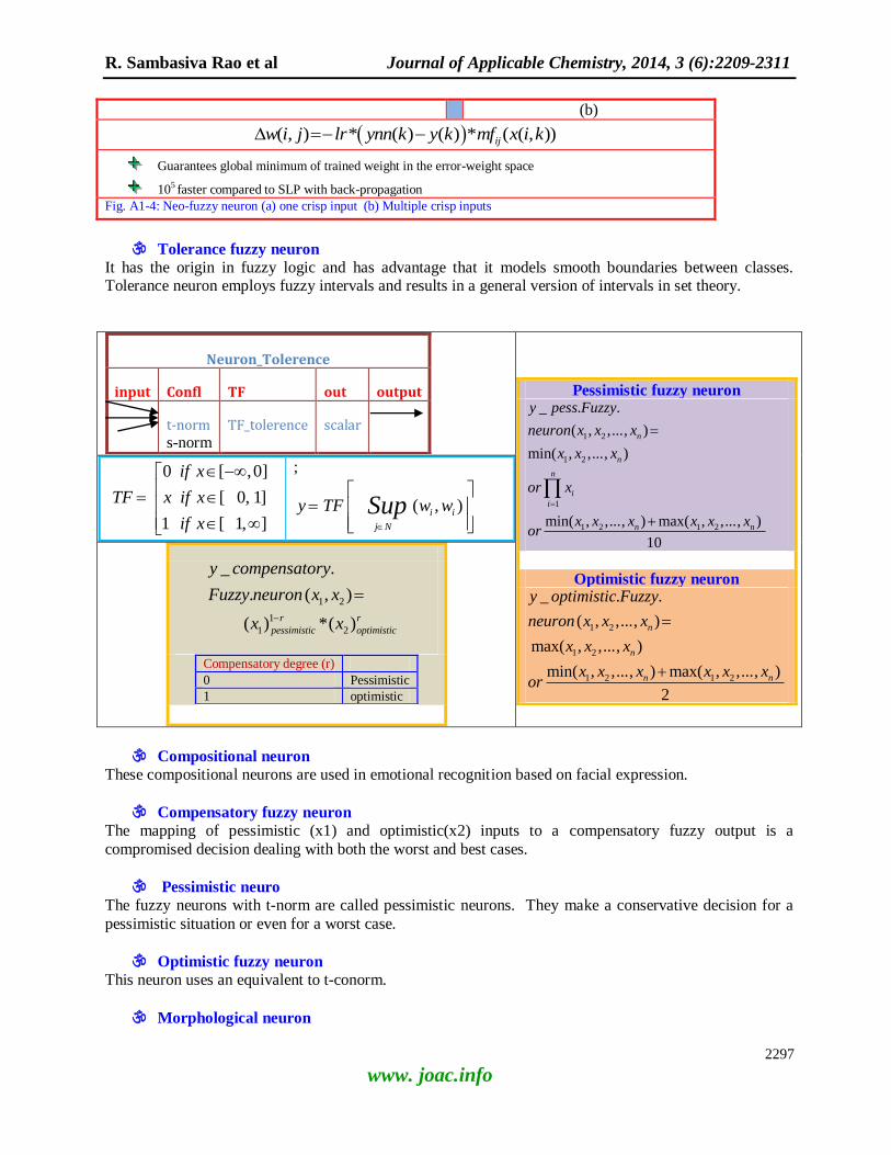
R. Sambasiva Rao et al Journal of Applicable Chemistry, 2014, 3 (6):2209-2311
2297
www. joac.info
(b)
( , ) * ( ) ( ) * ( ( , ))ijw i j lr ynn k y k mf x i k
Guarantees global minimum of trained weight in the error-weight space
105 faster compared to SLP with back-propagation
Fig. A1-4: Neo-fuzzy neuron (a) one crisp input (b) Multiple crisp inputs
Tolerance fuzzy neuron
It has the origin in fuzzy logic and has advantage that it models smooth boundaries between classes. Tolerance neuron employs fuzzy intervals and results in a general version of intervals in set theory.
Neuron_Tolerence
input Confl TF out output
t-norm s-norm
TF_tolerence scalar
Pessimistic fuzzy neuron
1 2
1 2
1
1 2 1 2
_ . .
( , ,..., )
min( , ,..., )
min( , ,..., ) max( , ,..., )
10
n
n
n
i
i
n n
y pess Fuzzy
neuron x x x
x x x
or x
x x x x x xor
Optimistic fuzzy neuron
1 2
1 2
1 2 1 2
_ . .
( , ,..., )
max( , ,..., )
min( , ,..., ) max( , ,..., )
2
n
n
n n
y optimistic Fuzzy
neuron x x x
x x x
x x x x x xor
0 [ ,0]
[ 0, 1]
1 [ 1, ]
if x
TF x if x
if x
;
( , )i i
j N
y TF w wSup
1 2
1
1 2
_ .
. ( , )
( ) *( )r r
pessimistic optimistic
y compensatory
Fuzzy neuron x x
x x
Compensatory degree (r)
0 Pessimistic
1 optimistic
Compositional neuron These compositional neurons are used in emotional recognition based on facial expression.
Compensatory fuzzy neuron
The mapping of pessimistic (x1) and optimistic(x2) inputs to a compensatory fuzzy output is a
compromised decision dealing with both the worst and best cases.
Pessimistic neuro
The fuzzy neurons with t-norm are called pessimistic neurons. They make a conservative decision for a
pessimistic situation or even for a worst case.
Optimistic fuzzy neuron
This neuron uses an equivalent to t-conorm.
Morphological neuron

R. Sambasiva Rao et al Journal of Applicable Chemistry, 2014, 3 (6):2209-2311
2298
www. joac.info
An elementary operation of mathematical morphology is performed in the neuron. Then activation (transfer) function operates on it [204]. Many of information granules viz. fuzzy sets, intervals and rough
sets are ordered in lattice frame and lattice theory provided underlying framework for mathematical
morphology. Thus, morphological-NNs, and fuzzy lattice neurocomputing are the order of day.
Stochastic Frame
Stochastic Neuron
In biological networks, probabilistic firing of neuron is also prevalent in addition to deterministic
constraint. The use of stochastic TF in the PE results in a stochastic neuron. Boltzmann machine uses
stochastic neurons and also introduces stochastic element in W. The transfer function of a stochastic neuron is an output probability against the input probability. The probabilities refer to a value of 1 on any
given clock cycle. It is used in pulsed RBF-NN.
Chaotic realm
Chaotic Neuron A chaotic neuron introduced in 1990s (table A1-19) exhibits a wide range of behavior similar to biological neurons. The output is in graded mode and refractoriness decays exponentially. NNs with chaotic neurons
have wide and flexible dynamics and arrive at global optima. It is used in Kohonen SOM and clustering
ability is increased through controlled randomness. By replacing conventional neurons of Kohonen SOM grid by chaotic neurons, a controlled randomness is developed in the self-organizing process. It improved
the ability of clustering task.
Table A1-19: Chaotic neurons
Aihara Dingle
4
0
( 1)
( ) _ * *
( ( )) )
t
delay
y t
u t scal par decayTF
refractFun y t delay threshold
1
1 * *( 1) 1 4*
( )* (1 ( ))
NP
i i
i
x wy t
y t y t
y(t) range : [0 to 1] ; u(t) : external input(stimulus)
at time t
If X'*W < 0.11 then output is chaotic
If X'*W range is [0.11 to 0.25] then output is periodic
If X'*W > 0.25 then output is a single value which
increases with X'*W
If X'*W > 0.75 then output is 1
Stochastic neuron
_
1
1 exp( 2* _ * )
TF stochastic
slope pdf x
Neuron_stochastic
input Confl TF out output
,inp w TF-stochastic scalar
Accurate approximation of Gaussian function
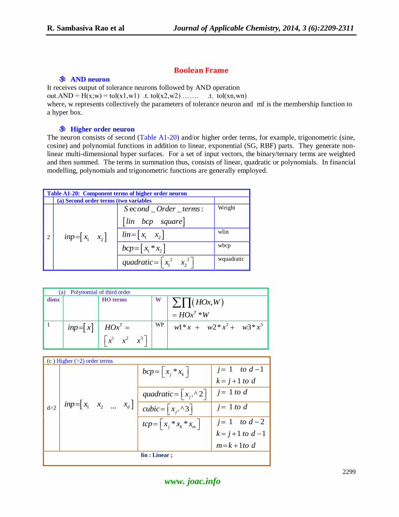
R. Sambasiva Rao et al Journal of Applicable Chemistry, 2014, 3 (6):2209-2311
2299
www. joac.info
Boolean Frame AND neuron
It receives output of tolerance neurons followed by AND operation out.AND = H(x;w) = tol(x1,w1) .t. tol(x2,w2) ……. .t. tol(xn,wn)
where, w represents collectively the parameters of tolerance neuron and mf is the membership function to
a hyper box.
Higher order neuron
The neuron consists of second (Table A1-20) and/or higher order terms, for example, trigonometric (sine,
cosine) and polynomial functions in addition to linear, exponential (SG, RBF) parts. They generate non-linear multi-dimensional hyper surfaces. For a set of input vectors, the binary/ternary terms are weighted
and then summed. The terms in summation thus, consists of linear, quadratic or polynomials. In financial
modelling, polynomials and trigonometric functions are generally employed.
Table A1-20: Component terms of higher order neuron
(a) Second order terms (two variables
2 1 2inp x x
ec _ _ :S ond Order terms
lin bcp square
Weight
1 2lin x x
wlin
1 2*bcp x x
wbcp
2 2
1 2quadratic x x
wquadratic
(a) Polynomial of third order
dimx HO terms W ,HOx W
*THOx W
1 inp x
1 2 3
THOx
x x x
WP 2 31* 2* 3*w x w x w x
(c ) Higher (>2) order terms
d>2 1 2 ... dxinp x x
*j kbcp x x
1 1
1
j to d
k j to d
.^ 2jquadratic x
1j to d
.^3jcubic x
1j to d
* *j k mtcp x x x
1 2
1 1
1
j to d
k j to d
m k to d
lin : Linear ;

R. Sambasiva Rao et al Journal of Applicable Chemistry, 2014, 3 (6):2209-2311
2300
www. joac.info
quadratic: square ;
bcp: binary cross product;
Second order : [square, bcp] ;
tcp: ternary cross product
Cubic: cube;
Lipson-Higher order neuron Lipson proposed tensors as another type of higher-order-neurons. Their order pertains to internal tensorial
order, but not the degree of output (table A1-21). This higher order neuron considers the covariance matrix
unlike a classical neuron. It simulates shapes with holes and detached areas. It captures higher order
information within a single neuron.
Table A1-21: Higher order neuron
(a) Second order components
Fourthorder tensor H H H H H Hx x x x R R
2 2
2 2
1 1* 2 1 1* 2
1* 2 2 1* 2 2
x x x x x x
x x x x x x
2 2
2
2 2
2 2
2
2 2
1 1* 2 1 1* 21 * 1* 2*
1* 2 2 1* 2 2
1 1* 2 1 1* 21* 2* 1 *
1* 2 2 1* 2 2
x x x x x xx x x
x x x x x x
x x x x x xx x x
x x x x x x
4 3 4 3
3 2 2 3 2 2
4 3 4 3
3 2 2 3 2 2
1 1 * 2 1 1 * 2
1 * 2 1 * 2 1 * 2 1 * 2
1 1 * 2 1 1 * 2
1 * 2 1 * 2 1 * 2 1 * 2
x x x x x x
x x x x x x x x
correct it
x x x x x x
x x x x x x x x
(b) First and second order components
Fourthorder tensor
2 2
2 2
1 1* 2 1 1 1* 2 1
1* 2 2 2 1* 2 2 2
1 2 1 1 2 1
x x x x x x x x
x x x x x x x x
x x x x
Lipson-Higher-order -NNs
Good stability
Excellent training performance even with Hebbian learning rule
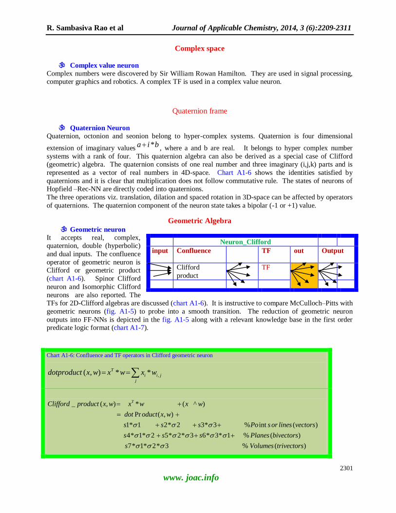
R. Sambasiva Rao et al Journal of Applicable Chemistry, 2014, 3 (6):2209-2311
2301
www. joac.info
Complex space
Complex value neuron
Complex numbers were discovered by Sir William Rowan Hamilton. They are used in signal processing, computer graphics and robotics. A complex TF is used in a complex value neuron.
Quaternion frame
Quaternion Neuron
Quaternion, octonion and seonion belong to hyper-complex systems. Quaternion is four dimensional
extension of imaginary values *a i b , where a and b are real. It belongs to hyper complex number
systems with a rank of four. This quaternion algebra can also be derived as a special case of Clifford (geometric) algebra. The quaternion consists of one real number and three imaginary (i,j,k) parts and is
represented as a vector of real numbers in 4D-space. Chart A1-6 shows the identities satisfied by
quaternions and it is clear that multiplication does not follow commutative rule. The states of neurons of Hopfield –Rec-NN are directly coded into quaternions.
The three operations viz. translation, dilation and spaced rotation in 3D-space can be affected by operators
of quaternions. The quaternion component of the neuron state takes a bipolar (-1 or +1) value.
Geometric Algebra Geometric neuron
It accepts real, complex, quaternion, double (hyperbolic)
and dual inputs. The confluence
operator of geometric neuron is Clifford or geometric product
(chart A1-6). Spinor Clifford
neuron and Isomorphic Clifford
neurons are also reported. The TFs for 2D-Clifford algebras are discussed (chart A1-6). It is instructive to compare McCulloch–Pitts with
geometric neurons (fig. A1-5) to probe into a smooth transition. The reduction of geometric neuron
outputs into FF-NNs is depicted in the fig. A1-5 along with a relevant knowledge base in the first order predicate logic format (chart A1-7).
Chart A1-6: Confluence and TF operators in Clifford geometric neuron
,( , ) * *T
i i j
j
dotproduct x w x w x w
_ ( , ) * ( ^ )
Pr ( , )
1* 1 2* 2 3* 3 % int ( )
4* 1* 2 5* 2* 3 6* 3* 1 % ( )
7* 1* 2* 3 % ( )
TClifford product x w x w x w
dot oduct x w
s s s Po s or lines vectors
s s s Planes bivectors
s Volumes trivectors
Neuron_Clifford
input Confluence TF out Output
Clifford
product
TF
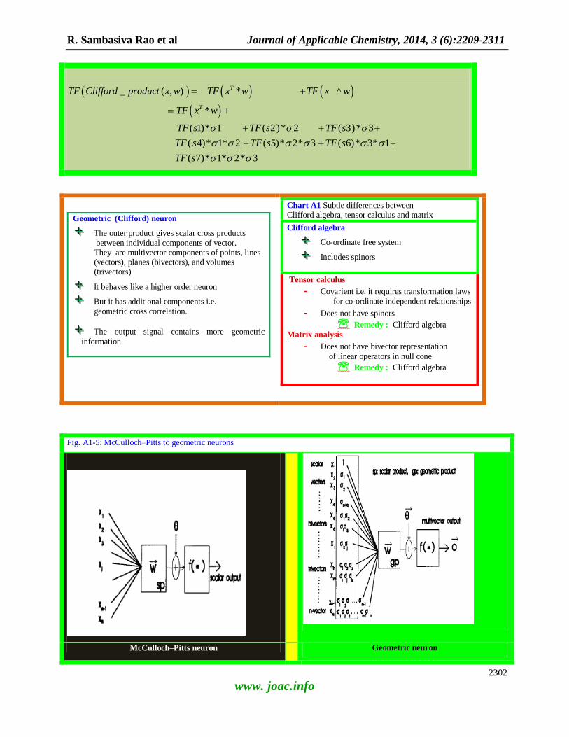
R. Sambasiva Rao et al Journal of Applicable Chemistry, 2014, 3 (6):2209-2311
2302
www. joac.info
_ ( , ) * ^
*
( 1)* 1 ( 2)* 2 ( 3)* 3
( 4)* 1* 2 ( 5)* 2* 3 ( 6)* 3* 1
( 7)* 1* 2* 3
T
T
TF Clifford product x w TF x w TF x w
TF x w
TF s TF s TF s
TF s TF s TF s
TF s
Geometric (Clifford) neuron
The outer product gives scalar cross products
between individual components of vector. They are multivector components of points, lines (vectors), planes (bivectors), and volumes (trivectors)
It behaves like a higher order neuron
But it has additional components i.e.
geometric cross correlation.
The output signal contains more geometric
information
Chart A1 Subtle differences between Clifford algebra, tensor calculus and matrix
Clifford algebra
Co-ordinate free system
Includes spinors
Tensor calculus
- Covarient i.e. it requires transformation laws
for co-ordinate independent relationships
- Does not have spinors
Remedy : Clifford algebra
Matrix analysis
- Does not have bivector representation
of linear operators in null cone
Remedy : Clifford algebra
Fig. A1-5: McCulloch–Pitts to geometric neurons
McCulloch–Pitts neuron Geometric neuron

R. Sambasiva Rao et al Journal of Applicable Chemistry, 2014, 3 (6):2209-2311
2303
www. joac.info
Chart A1-7: Quaternion neuron, NN and FF_NN
_ 1 * 2 * 3 * 4x quaternion x i x j x k x
x1,x2,x3 and x4
: real numerical values
1 2 3, , : Orthonormal
basis vectors
_ :( 1, 2, 3, 4)
: 1, 2, 3, 4
x quaternion x x x x
x x x x
2 3
3 1
1 2
*
*
*
i
j
k
2 2 2 1 * *
* * ;
* * ;
* * ;
i j k i j k
i j j i
j k k j
k i i k
Equivalence of Geometric NNs with FF-NNs If G(0,2,0) Then quaternion-valued NN
If G(1,1,0) Then hyperbolic MLP
If G(0,3,0) Then hyperbolic (double)
quaternion-valued RBF
If G(3,0,0) Then works in the entire
Euclidean 3-D geometric algebra
If G(4,1,0) Then works in the horosphere If G+(3,3,0)
Then bivector null cone
KB for input of a geometric neuron
If I2 = -1 Then complex numbers
If I2 = 1 Then double or hyperbolic numbers
If I2 = 0
Then dual numbers (a degenerated geometric algebra)
Artificial neurons (An ant) not very far away from biological neurons
Bifurcating neuron Biological inspiration of bifurcating neural activity is from olfactory systems. The state of olfactory bulb
wanders in a high dimensional chaotic attractor space in the absence of any detectable odor. When an odor
is found, the input through nose shifts to one of the low
dimensional attractors. It corresponds to a wing of recognized specific odour. The coherent activities in
brain measured in gamma-band centered around 40 Hz are
of recent interest in olfactory systems of cat and rat. The primary visual cortex in the cat, monkey and EEGs of
human brain above association and motor areas belong to
this category. A bifurcating neuron using a third order iterate of
quadratic logistic map. The external input is used to govern the dynamics. A certain input shifts the
dynamics of a neuron from chaos to one of stable fixed point, while the rest are mapped to chaotic or
Chart A1-8: Bifurcating neuron
It functions as an amplitude-phase converter
Inherent capacity is a coincidence detector
Exhibits associative memory of multiple
analogue patterns, volume holographic memory
Switches to different phases of its memory space
with change in frequency of the coherent modulation i.e. context sensitive memory

R. Sambasiva Rao et al Journal of Applicable Chemistry, 2014, 3 (6):2209-2311
2304
www. joac.info
periodic output. Bifurcating neuron is a model of a neuron augmented by coherent modulation from its environment (chart A1-8).
Hodgkin-Huxley neuron Alan Lloyd Hodgkin and Andrew Huxley in 1952 proposed the first scientific neuron model to mimic
biological neuron closely. It describes how action potentials are developed and propagated. The exchange
of neurotransmitters, chemical moieties in the synaptic gap promote communication of signals. The
membrane of the cell consists of voltage dependent channels. The conductance of sodium and potassium ions through these channels results in the membrane current of a neuron. The other
ionic currents are described by ohmic leakage contribution. It
models membrane potential with detailed spike generation based on development of response with changes in several ion channels. The
accuracy of the model increases by incorporating the geometry of
compartments of the neuron. A few novel advanced processes are incorporated in FitzHugh-Nagumo (1961-1962) and Hindmarsh-Rose
(1984) models.
Spiking neuron A spiking neuron with excitatory and inhibitory signals
of a train of stimulated signals with and without noise was
proposed. The NN using these neurons performed well in modeling somato sensory system (Table A1-22) and
grouping of objects of interest in diabetic retinopathy
images. The input (spikes) signals enter the neuron
through synaptic connection. It increases the conductance of synapse with changes in post synaptic potential. The
weighted sum of all excitatory and inhibitory synaptic
conductances results in a stimulus of a train of spikes. Absolute refractory period is a short interval immediately
after generation of spike. During this period,
the neuron is incapable of responding to any further stimulation (of input). Then, it follows relative refractory period. Here, only very strong stimulations are responded. Post synaptic potential of the neuron
is a result of increased synaptic conductance. They used
MacGregor's integrate-and-fire model which takes into
account threshold membrane potential and potassium channel response. This is simpler compared to Hodgkin-Huxley model in generation of spike. The
excitation and inhibition reflect (model) individual channel.
Oscillatory Neuron
Inoue and Nagayoshi proposed an oscillatory neuron. It is made up of excitatory as well as inhibitory
coupled oscillators. This neuron deals with noisy and chaotic information. Its oscillatory function is described by frequency, phase and amplitude. Oscillatory neurons are not widely used in artificial NNs.
This is partially as a result of the feel that many numerical tasks are sufficiently dealt by hither to known
artificial neurons. Further, the binary logic hardware structure is not comfortable to implement oscillatory
model.
Leaky integrator neuron
The input to output transformation of leaky integrator neuron and knowledge base are given in chart A1-9.
Hodgkin-Huxley neuron
- Computationally intense even from
standpoint of today's hard/software
- Mechanistic-physical model of
biological neuron is complex
Table A1-22: Architecture of Spiking-NN used for
classification of retinopathy images
Layer Model of architecture
Sensory Tactile receptors on the skin
9 x 9
Sub cortical layer-1 Spinal card and brain stem
9 x 9
Sub cortical layer-2 Thalamus 21 x 21 Exc 9 x 9 Inh
Cortical layer Cortex 21 x 21 Exc 9 x 9 Inh
Exc: excitatory neurons; Inh: inhibitory neurons
If Stimulus is strong i.e. exceeds the threshold Then The neuron fires

R. Sambasiva Rao et al Journal of Applicable Chemistry, 2014, 3 (6):2209-2311
2305
www. joac.info
Appendix A1c: Accumulation (confluence) operator
The confluence operators in use are summation, product,
power for crisp values, and minimum/maximum in fuzzy domain and so on.
Appendix A1d: Boolean gates
XOR: From the figure (Fig. A1-6), it is clear that it is not a linearly separable problem and thus direct I/O nets
(MC-NN) cannot solve the task. This simplest non-linear
problem was solved with the introduction of a layer of neurons with non-linear (sigmoid) transfer function in
between the input and output layers. This net is
popularly known as SLP_NN, or in other words MLP_NN with only one hidden layer. Figure A1-6
incorporates multi-dimensional XOR data.
Case 1: SLP with one hidden neuron and direct I/O connections gracefully solves XOR. To be brief, a non-
linear neuron generates non-linear discriminating
function.
Case 2 : Two hidden neurons in the hidden layer of SLP
(without direct IO connections) is also adequate.
Fig. A1-6: Boolean gates
Input Output of Boolean gates
1 2 3 4 5 6 7 8 9 10 11 12 13 14 15 16
1 1 0 1 0 0 0 1 0 0 1 1 0 0 1 1 1 1 0 0 0 0 1 0 0 1 1 0 0 0 1 1 0 1 1 1
1 0 0 0 0 1 0 0 1 1 1 0 0 1 1 0 1 1 0 1 0 0 0 0 1 0 0 1 0 1 1 1 1 1 0 1 nor and xnor xor or nand
Input Output
x1 x2 OR NOR
(not OR)
XOR XNOR
(not XOR)
yOR yNOR yXOR yXNOR
0 0 0 1 1 0 1 0 1 0 0 1 0 1 1 0 0 1 1 1 1 0 1 0
0 0.2 0.4 0.6 0.8 10
0.2
0.4
0.6
0.8
1XOR
0
0.5
1
0
0.5
10
0.5
1
1 1.5 2 2.5 31
1.5
2
2.5
3
3.5
4
1
2
3
0
2
40
0.5
1
Chart A1-9: Leaky integrated neuron
At time t, x(t) is input, out.y(t) = TF(x'*w) At time t+1, input is x(t+1), net input = x(t+1) + feedback = x(t+1) +TF(x'*w)
output at t+1= y(t+1) = TF([x(t+1) +TF(x'*w)])
If there is no external input at the
time instance t+1, (i.e. x(t+1) = 0),
Then y(t+1) = TF([TF(x'*w)]) = function(y(t))
If feedback is an exponential decay function & x = 1
Then output repeats it (y = 1)
If input signal is not present Then output value decreases over
time
It remembers event x at least for some time i.e. last input signal is kept and decays exponentially
- Forgets remembered event in far
distant future time
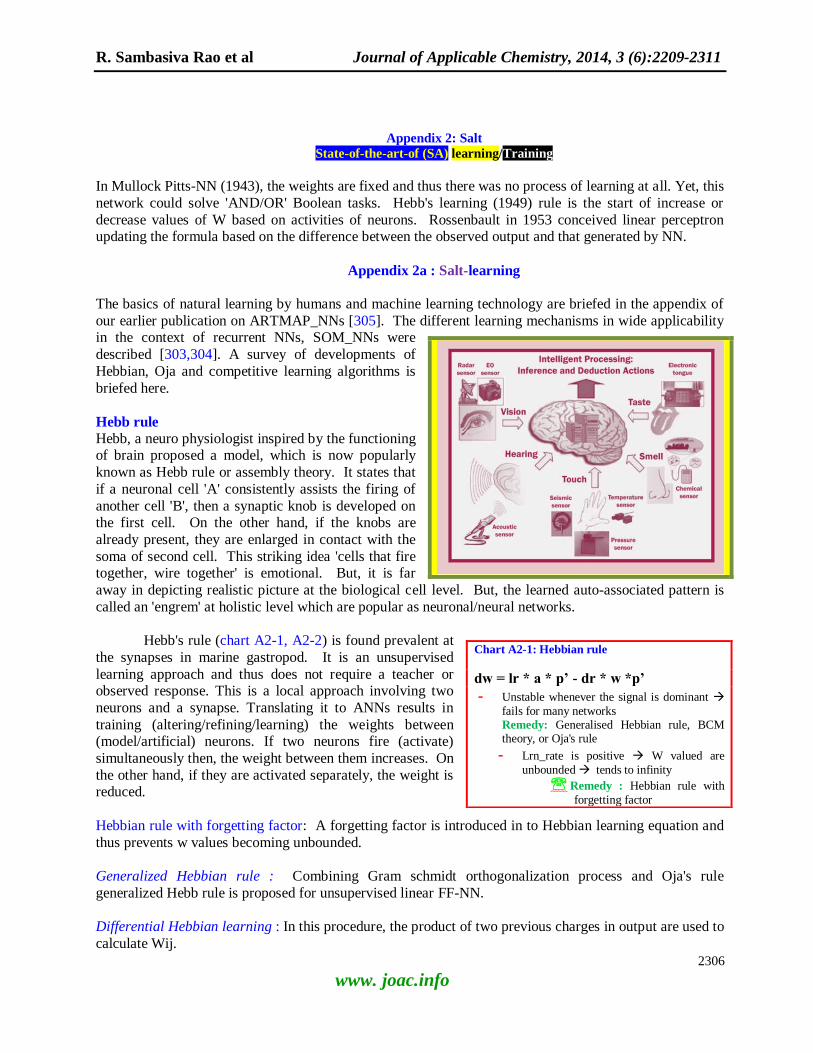
R. Sambasiva Rao et al Journal of Applicable Chemistry, 2014, 3 (6):2209-2311
2306
www. joac.info
Appendix 2: Salt
State-of-the-art-of (SA) learning/Training
In Mullock Pitts-NN (1943), the weights are fixed and thus there was no process of learning at all. Yet, this
network could solve 'AND/OR' Boolean tasks. Hebb's learning (1949) rule is the start of increase or
decrease values of W based on activities of neurons. Rossenbault in 1953 conceived linear perceptron updating the formula based on the difference between the observed output and that generated by NN.
Appendix 2a : Salt-learning
The basics of natural learning by humans and machine learning technology are briefed in the appendix of
our earlier publication on ARTMAP_NNs [305]. The different learning mechanisms in wide applicability in the context of recurrent NNs, SOM_NNs were
described [303,304]. A survey of developments of
Hebbian, Oja and competitive learning algorithms is
briefed here.
Hebb rule
Hebb, a neuro physiologist inspired by the functioning of brain proposed a model, which is now popularly
known as Hebb rule or assembly theory. It states that
if a neuronal cell 'A' consistently assists the firing of
another cell 'B', then a synaptic knob is developed on the first cell. On the other hand, if the knobs are
already present, they are enlarged in contact with the
soma of second cell. This striking idea 'cells that fire together, wire together' is emotional. But, it is far
away in depicting realistic picture at the biological cell level. But, the learned auto-associated pattern is
called an 'engrem' at holistic level which are popular as neuronal/neural networks.
Hebb's rule (chart A2-1, A2-2) is found prevalent at
the synapses in marine gastropod. It is an unsupervised
learning approach and thus does not require a teacher or observed response. This is a local approach involving two
neurons and a synapse. Translating it to ANNs results in
training (altering/refining/learning) the weights between (model/artificial) neurons. If two neurons fire (activate)
simultaneously then, the weight between them increases. On
the other hand, if they are activated separately, the weight is reduced.
Hebbian rule with forgetting factor: A forgetting factor is introduced in to Hebbian learning equation and
thus prevents w values becoming unbounded.
Generalized Hebbian rule : Combining Gram schmidt orthogonalization process and Oja's rule
generalized Hebb rule is proposed for unsupervised linear FF-NN.
Differential Hebbian learning : In this procedure, the product of two previous charges in output are used to
calculate Wij.
Chart A2-1: Hebbian rule
dw = lr * a * p’ - dr * w *p’
- Unstable whenever the signal is dominant
fails for many networks Remedy: Generalised Hebbian rule, BCM theory, or Oja's rule
- Lrn_rate is positive W valued are
unbounded tends to infinity
Remedy : Hebbian rule with
forgetting factor

R. Sambasiva Rao et al Journal of Applicable Chemistry, 2014, 3 (6):2209-2311
2307
www. joac.info
Oja learning rule or modified Hebbian learning
The synaptic strengths between the neurons in the brain change over time. This inspired Oja to propose a
computational form in 1982. Thus, it is a modified Hebbian rule though multiplicative normalization.
Chart A2-2: Output of om_ref_JAVATYP.m
Hebb learning B. Lu, A. Dibazar, T. W. Berger
Noise-robust acoustic signature recognition using nonlinear Hebbian learning
Neural networks 23(10)(2010)1252-1263
D.O. Hebb, W. Penfield Human behaviour after extensive bilateral removal from the frontal lobes
Archives of Neurology and Psychiatry
44(1940)421–436
D.O. Hebb Distinctive features of learning in the higher animal
J. F. Delafresnaye (Ed.): Brain Mechanisms and Learning .
Oxford University Press, (1961)
London.
D.O. Hebb The organization of behavior
New York, Wiley (1949)
om_ref_JAVATYP.m
object module (om_ ) reference (ref_)
Journal Author Volume And (JAVATYP) Title Year Pages
matlab function(.m)
The stability of Oja's learning rule is derived for Lyapunov function. Here, the change in pre-
synaptic w of a single neuron is calculated. The weights are normalized between zero and one. A value of zero corresponds to no weight or (no connection), while one represents that only the corresponding input
neuron has all the weight. Oja considered a case resulting in a quadratic form. Of course, linear and any
other non-linear form also has the same theoretical rigor and generality. The output activation function can be non-linear and non-static, but it should be continuously differentiable with respect to x and w. Although
there is not yet experimental evidence of this rule in biological NNs, it is applied with great success in
many image and speech recognition/synthesis and binocular vision systems.
PCs from Oja’s rule
Applying Oja's rule to a single neuron, the first PC is obtained. Multi-Oja-NN with generalized Hebbian
rule and more number of neurons extracts all PCs and Eigen values.
Widrow-Hoff learning rule
The least mean squares filter (LMS) of Widrow is used to train ADALINE (ADAptive LInear Neuron) and MADALINE (Multiple ADALINE) NNs.
Adaptive learning algorithm: Hara analyzed a learning algorithm employing a margin Kappa a la
Gardner in NNs (KB. A2-1)
Add-if-silent rule

R. Sambasiva Rao et al Journal of Applicable Chemistry, 2014, 3 (6):2209-2311
2308
www. joac.info
Fukushima introduced add-if-silent learning rule for neocognitron model of robust pattern recognition (chart A2-3).
Winner-kills-loser (WKL) It is a competitive learning rules introduced in the context of training neocognitron neural network. Now,
WKL with three thresholds outperforms winner-takes all (WTA) learning in recognition of
distorted/blurred/tilted digits/alphabets.
KB. A2-1: Effect of kappa
on type of learning
If kappa = 0 Then perceptron learning
If kappa
Then Hebbian learning
If 1.51*kappa l
Then superior generalization compared to Hebbian learning
Chart A2-4: Test data sets for border Pairs
learning algorithm
Classification XOR Iris
Pattern recognition
triangles image
Digits Handwritten Pen-Based
noisy patterns
Chart A2-5: Deep_NNs and deep_learning
Deep_NNs
Complex MLP structures
Contains richer information
Improved representation ability compared with traditional data-driven models
Deep learning
Semi-supervised o All available process data can be
utilized
Efficient with massive data in practice
Chart A2-3: Add- if-silent rule
Stable
Simple
High recognition rate
Independent of scale of network
Iteriative-EKF learning rule
Iterative extended Kalman filter learning rule is a continuous learning rule derivable from Bayesian
framework. The object function is the minimization of sum of MSE and regularization. It is applicable
when the non-linear relationship gradually changes over time. The algorithm is found to be superior to on-
line BP-EKF while comparable with Black-Scholes benchmark model for German stock exchange index data.
Border Pairs learning algorithm Ploj et al. [257] used border pairs learning algorithm for MLP_NN for a large number of classification and
pattern recognition tasks. The learning is affected separately layer as well as neuron wise. This method
finds a near-minimal architecture, a desirable feature in NN activity (chart A2-4).
Deep_NN Learning algorithm The random neural network was introduced in 1989. The learning algorithms are reviewed along with
application for classification. The future prospective research ventures identifying the gaps and holes in
the field are emphasized. Sussner and Esmi [204] reported competitive learning with winner-take-all mechanism for morphological perceptrons. The results of this method are compared with MLP, fuzzy
lattice neurocomputing , kNN and decision trees. The deep_NNs are trained with deep learning strategy
(chart A2-5) and applied to calculate heavy diesel 95% cut point of a crude distillation unit (CDU).
R. Sambasiva Rao et al Journal of Applicable Chemistry, 2014, 3 (6):2209-2311
2309
www. joac.info
Deep_NNs are not simple MLPs and also latent variable models. Thus, they handle highly correlated process variables.
Wake and sleep algorithm The two phases –wake and sleep—are local learning processes. They are repeated alternatively to
reconstruct the input patterns at the output layer of a 3-layer auto-coder. Katayama used Hinton‘s wake –
sleep algorithm to explain response properties of medial superior temporal MST neurons for binary Q = 2
and multiple 3Q states. The recognition model represents the architecture from medial temporal MT
area to MST area.
Correlation learning
The correlational learning is useful for NNs with discrete input and output values. From the degree of
overlap of input patterns a separability factor is defined. The binary values zero and one in a subset of input cells are represented by a uni-directional graph. This is a generalized topological mapping preserving
the input pattern relation.
Negative correlation learning In unbiased individual NNs the errors between them are uncorrelated. A negative correlation learning to
design and train an ensemble of NNs simultaneously and interactively was proposed. Introduction of
correlation penalty terms in the object error function is the basis of negative correlation learning. Training with this algorithm results in negatively correlated NNs with increased generalization
Learning in NNs from statistical framework perspective In statistical or mathematical modeling, data is fit into the user chosen model. If it is not adequate, another
model is tried. This process is continued till an adequate (not even ambitious) model is arrived at. On the
other hand, NNs learn from data set and at the end of this phase, a (blackbox/implicit) model is developed.
Learning in NNs also is an estimation of an unknown probability distribution { / ,p y x W } from
statistical point of view.
Arriving at W matrix with a chosen optimization function is called training in NN terminology. The assumption is the existence of a functional relationship between X and y, although not known to the
user. The weights of NN are estimated from a set of NP training patterns satisfying the chosen
optimization function. The solution procedure adapted depends upon difficulty of data structure, ease of operation of a method in a package and most important mind set etc. A statistical model is realizable if
and only if the parameters are uniquely determined from its behavior or mapping from W to / ,p y x W
be one to one. In the conventional statistical theory, Bayesian posterior pdf converges to Gaussian
distribution and generalized error is proportional to the number of parameters. Watanabe pointed out that
conventional statistical asymptotic theory couldn‘t be applied to MLP_NN and RBF_NN or Gaussian
mixture NNs. It is due to the fact that Fisher information matrices are not positive definite and Ws are non-identifiable. And, going deep into statistical distribution of static/dynamic parameters/ noise in data,
non-parametric models and distribution free data processing are beyond the scope here. Thus, from broad
perspective, the iterative refinement of parameter models in mathematical optimization/statistical regressions, learning of connection weights in historical NNs and training of Ws in MLP_NN, RBF_NN
and Rec_NNs are similar but for terminology.
Appendix A2b: Salt-Training
Back propagation The typical developments in back propagation algorithm are briefed in Chart A2-6, table A2-1, Alg. 2-1
and Alg. A2-2.

R. Sambasiva Rao et al Journal of Applicable Chemistry, 2014, 3 (6):2209-2311
2310
www. joac.info
Chart A2-6: Typical BP algorithms
Backpropagation (BP)
Std "Vanilla‖
ThroughTime
WeightDecay
Batch
Batch ThroughTime
Batch TimeDelay
Chunk
weight & bias
weight & bias & one vector at a time
Cum-delta
Delta Bar Delta
Delta rule
Directed
random search
Ext.DBD
Max Prop
Momentum
Norm-cum-delta
Quick Propogation
Quickprop
Quickprop
throughTime
Rprop in CC
Alg. A2-1 : Pseudo inverse training in MLP [11]
Number of hidden neurons = nlayer Yapp = X
For layer = 0 to nlayer Cal. inv_Yapp = pinv(Yapp)
ESS = [Norm(Y_layer – inv(Y_layer) – I)]2
While ESS > Error_tol W_layer = inv(Y_layer)
% Feed forward the result to the next layer
Y(layer+1) = TF * (Y_layer *
W_layer) Inv_Y(layer+1) = pinv(Y(layer+1)) End while
End layer
YNN = TF [TF[TF(Yap*Wap)] * W1] …..* Wnlalyer]
Alg. A2-2: BP for RBF
Initialization of network For epoch : 1 to max_epoch
Repeat for input : 1 to all input vectors
compute the network output by proceeding forward layer by layer
calculate (error) residual gradient vs parameters layer by layer starting from output
update parameter_w
end % input
end % epoch
Expert Opinion (EO_KB)
Momentum term has a little effect in
training RBF
Sigmoid as TF_OL improves training
CV for better generalization
Table A2-1: Chronological developments in learning algorithms (BP) for Ws of NNs
Year Limitations/ improvement/ modification of BP Comment Ref.
1994 - Back propagation error surface is like
ravine
Remedy: difference of gradients is used as acceleration algorithm to escape from ravine
66
1994 Davidson's LS One step ahead prediction 67
1995 - Adaptive agent contains not worker but a
critic.
Remedy: Neural critic adopts a new learning alg 63
1995 Acceleration of momentum by constrained optimization
Optimizes alignment of weights successively. FF MLP 64
2000 If input has errors Then new cost function based on errors
Remedy: Stochastic frame work Marquardt B P for errors in x and y
76

R. Sambasiva Rao et al Journal of Applicable Chemistry, 2014, 3 (6):2209-2311
2311
www. joac.info
2000 - Block training reduced sensitivity 72
2001 Linear constraints are introduced into error function
69
2001 First and higher derivatives included based on regularization
Improvement of generalization 53
2001 Maximum inter quartile range used Active learning reduces amount of data selection 74
2001 Blowing up technology used in hierarchical learning.
Bayesian GE of HLM is smaller than that in regular
statistical module
74