Journal of Applied Geophysics 74 (2011) 194–204

Contents lists available at ScienceDirect

Journal of Applied Geophysics

j ourna l homepage: www.e lsev ie r.com/ locate / jappgeo

Interpretation of magnetic data in the Sinop area of Mid Black Sea, Turkey, using tiltderivative, Euler deconvolution, and discrete wavelet transform

B. Oruç a,⁎, H.H. Selim b

a Kocaeli University, Engineering Faculty, Department of Geophysical Engineering, Umuttepe Campus, 41380 İzmit/Kocaeli, Turkeyb Kocaeli University, Engineering Faculty, Department of Geological Engineering, Umuttepe Campus, 41380 İzmit/Kocaeli, Turkey

⁎ Corresponding author. Fax: +90 262 3352812.E-mail addresses: bulent.oruc@kocaeli.edu.tr (B. Oru

(H.H. Selim).

0926-9851/$ – see front matter © 2011 Elsevier B.V. Adoi:10.1016/j.jappgeo.2011.05.007

a b s t r a c t

a r t i c l e i n f o

Article history:Received 8 March 2011Accepted 25 May 2011Available online xxxx

Keywords:Magnetic anomaliesTilt derivativeEuler deconvolutionDiscrete wavelet transformStructural lineaments

The identification of lineaments in magnetic anomaly data is an important step in interpretation. In this paper,three methods for locating magnetic lineaments are applied to total field magnetic anomaly data of the Sinoparea of mid Black Sea, northern Turkey. Based upon the variation in magnetic lineaments, structural map ofthe study area was obtained. The tilt derivative (TDR), Euler deconvolution (ED) and discrete wavelettransform (DWT) have been of great utility in the interpretation of magnetic anomaly data. These threemethods were applied to enhance magnetic anomalies due to anomalous sources in part of the basementcomplex of study area. The TDR obtained from the magnetic anomaly reduced to pole (RTP) was designed tomap geologic contacts. The source boundaries and depths are determined from the zero contours, and the halfdistance between ±π/4 contours or the distance between zero and +π/4 or −π/4 contour of TDR,respectively. The ED technique is used to estimate the source depth at the semi-infinite contact location. TheDWT technique was carried out to infer the substructure orientation. The direction of maxima and minimacoefficients of the horizontal, vertical and diagonal decompositions of the DWT works in imaging thehorizontal locations of the anomalous sources. The results allow us to image and characterize subsurfacelineaments for the survey area.

ç), haluk.selim@kocaeli.edu.tr

ll rights reserved.

© 2011 Elsevier B.V. All rights reserved.

Contents

1. Introduction . . . . . . . . . . . . . . . . . . . . . . . . . . . . . . . . . . . . . . . . . . . . . . . . . . . . . . . . . . . . . . . 02. Geological setting. . . . . . . . . . . . . . . . . . . . . . . . . . . . . . . . . . . . . . . . . . . . . . . . . . . . . . . . . . . . . 03. Magnetic data . . . . . . . . . . . . . . . . . . . . . . . . . . . . . . . . . . . . . . . . . . . . . . . . . . . . . . . . . . . . . . 0

3.1. Data enhancement . . . . . . . . . . . . . . . . . . . . . . . . . . . . . . . . . . . . . . . . . . . . . . . . . . . . . . . . . 03.1.1. TDR image . . . . . . . . . . . . . . . . . . . . . . . . . . . . . . . . . . . . . . . . . . . . . . . . . . . . . . . . 03.1.2. Euler deconvolution solutions . . . . . . . . . . . . . . . . . . . . . . . . . . . . . . . . . . . . . . . . . . . . . . . 03.1.3. Two-dimensional DWT . . . . . . . . . . . . . . . . . . . . . . . . . . . . . . . . . . . . . . . . . . . . . . . . . . 03.1.4. Comparison of ED with TDR and DWT images. . . . . . . . . . . . . . . . . . . . . . . . . . . . . . . . . . . . . . . . 0

3.2. Delineation of magnetic features . . . . . . . . . . . . . . . . . . . . . . . . . . . . . . . . . . . . . . . . . . . . . . . . . . 04. Conclusions . . . . . . . . . . . . . . . . . . . . . . . . . . . . . . . . . . . . . . . . . . . . . . . . . . . . . . . . . . . . . . . 0Acknowledgments . . . . . . . . . . . . . . . . . . . . . . . . . . . . . . . . . . . . . . . . . . . . . . . . . . . . . . . . . . . . . . . 0References . . . . . . . . . . . . . . . . . . . . . . . . . . . . . . . . . . . . . . . . . . . . . . . . . . . . . . . . . . . . . . . . . . 0

1. Introduction

An important objective in the interpretation of potential field data isto improve the resolution of observed data. In magnetic prospecting, in

areas of limited exposure, delineating lateral change in magneticsusceptibilities provides information not only on lithological changesbut also on structural trends. Especially, mapping the edges of causativebodies is fundamental to the application of potential field data togeological mapping. The edge detection techniques are used todistinguish between different sizes and different depths of thegeological discontinuous. The derivatives of magnetic data are used toenhance the edges of anomalies and improve significantly the visibility

195B. Oruç, H.H. Selim / Journal of Applied Geophysics 74 (2011) 194–204

of such features. Many techniques for mapping have been developed todelineate structural features from magnetic data. Cordell and Grauch(1985) suggested a method for the location of the horizontal extents ofthe sources from the maxima of the horizontal gradient of thepseudogravity computed from the magnetic anomalies. Finding themaxima is then efficiently done with the curve-fitting approach ofBlakely and Simpson (1986).

The wavelet transform has been introduced into the geophysicalfield (Foufoula-Georgiou and Kumar, 1994) as a powerful analysistechnique. In contrast to the large number of studies into waveletmethods for seismic applications, there appears to be a relativelysmall amount of published research into wavelet methods forpotential fields. Moreau et al. (1997) applied the DWT analysis tothe case of gravity or magnetic anomalies, using wavelets built on thePoisson kernel. Fedi and Quarta (1998) used thewavelet transform forthe separation of regional and residual fields. Hornby et al. (1999)have used the wavelet transform to the analysis of gravity data for thecharacterization of geological boundaries. Ridsdill-Smith and Dentith(1999) has separated aeromagnetic anomalies usingwavelet matchedfilters. Moreau et al. (1999) have developed an efficient technique foridentification of sources of potential fields. The DWT can be employedto transform the potential field data in the space scale domain (Fediand Quarta, 1998; Moreau et al., 1997, 1999) without any a prioriinformation. Li and Oldenburg (2003) have demonstrated theapplication of the wavelet domain to be inversion of magnetic data.Albora et al. (2004) have applied the DWT to estimate the boundariesof an archeological site.

In the last few years there have been a number of methodsproposed to help normalize the signatures in images of magnetic dataso that weak, small amplitude anomalies can be amplified relative tostronger, larger amplitude anomalies. Verduzco et al. (2004) havedeveloped tilt derivative from gravity or magnetic field anomaly mapand suggested using the HGMof the tilt derivative as an edge detector.Keating and Pilkington (2004) have showed that the HGM of the tiltderivative is related to the local frequency. Wijns et al. (2005) use theanalytic signal amplitude to normalize the total horizontal derivative.Cooper and Cowan (2006) have used tilt angles which act asnormalized horizontal derivatives to detect the edges of anomaloussources. Salem et al. (2008) have developed a new method forinterpretation of gridded magnetic data based on the Tilt derivative,without specifying prior information about the nature of the source.

The main goal of this work is to analyze magnetic anomaly data toidentify possible lineaments in the Sinop basin area, mid Black Sea,Turkey. Our pattern recognition criteria are based on the TDR, ED, andDWT decompositions obtained from RTP anomaly data. All threemethods agree closely in determining the horizontal locations ofcontacts; the first two also give similar results for source depths.

2. Geological setting

The Black Sea is a large marginal sea located within the Alpineorogenic belt, surrounded by compressive tectonic belts, the Pontidesorogeny in the south, Caucasus in the northeast and Crimean Range inthe north (Çiftçi et al., 2003). It is located on the western flank of theactive Arabia–Eurasia collision and north of the North Anatolian Fault(NAF) that permits the tectonic escape of Anatolia (Rangin et al.,2002). The region was under the effect of compressive forces in thedirection of North Northeastern–South Southwestern between UpperCretaceous–Upper Miocene and at the end of the Miocene, thisactivity was suppressed by the activity of North Anatolian Fault (NAF)system (Özhan, 2004). As shown in Fig. 1a, the Black Sea basincomprises western and eastern Black Sea subbasins, which areseparated by a regional high, the mid Black Sea Ridge, which isdivided into two parts, the Andrusov Ridge in the north and theArchangelsky Ridge in the south (Dondurur and Çiftçi, 2008).

Gökaşan (1996), Özhan (2004), and Yılmaz et al. (1997) havereported the geological evolution of Black Sea in land and sea areas.The Sinop Basin is located between the Archangelsky Ridge and theTurkish coastline (Fig. 1a) and has been affected by late Miocenenormal faults along the Turkish margin and the Archangelsky Ridge(Rangin et al., 2002). The overall compressional deformation of theSinop Basin was superimposed onto the footwall block forming theArchangelsky Ridge (Çiftçi et al., 2003). In Sinop peninsula, Mioceneaged sandy limestones overly Upper Crateceous agglomerates(Fig. 1b).

3. Magnetic data

The total intensity magnetic field dataset provided by the TurkishNavy Department of Navigation, Hydrography and Oceanographywere recorded using the cesium-vapor marine magnetometer withsensitivity at 0.004 nT. The acquisition of magnetic data in thesouthern part of the Sinop basin was carried out along a north–south-striking profile perpendicular to the main tectonic structures.The magnetic data was acquired to allow structural interpretations tobe carried out in regions where little or any data had not previouslyexisted. Fig. 2a shows the total field anomaly map covering a portionof the Sinop basin (onshore partially). In the study area, the magneticsignature is generally smooth, with anomalies of different wave-lengths and amplitudes, denoting the different magnetic contents ofthe Sinop basin infill.

A correlation is seen between linear and circular patterns on theanomaly map. The anomaly map shows high amplitude and highwavenumber anomalies in the region. The high gradient contourssuggest fault like structures in the central part of the study area inWNW–ESE direction (Fig. 2a). This major trend was observed alongthe border of prominent high-amplitude linear anomalies withcontrasting magnetic properties.

3.1. Data enhancement

The total field anomaly map was processed to prepare for analysisand interpretation. The reason for this pre-processing is that themajor features in the data which may be defined by the edges andminor features that are not easily seen in the original image are todetect. Before applying the TDR, ED and DWT methods, the total fieldanomaly data were converted to RTP using a magnetic inclination of60° and a declination of 5.5°. Thus, the RTP reduces the effect of theEarth's ambient magnetic field and provides a more accuratedetermination of the position of anomalous sources. It is thereforeunderstood that the total magnetization direction is equivalent to thatof the current inducing filed. As is well known, this assumption statesthat the direction of magnetization in the anomalous sources lies inthe same direction as the local magnetic field. Unfortunately, we hadto ignore the remanent magnetization because of a lack of relevantinformation. Thus the real data example demonstrated in this sectioncould correspond to the case of zero remanent magnetization.However, in the case of the presence of strong remanent magnetiza-tion, this will adversely affect the interpretation of the magneticanomaly data and lead to erroneous size or shape.

The RTP signature of the Sinop Basin is marked by a rugged reliefwith positive and negative anomalies of several wavelengths andamplitudes, with values ranging between −900 and 1400 nT(Fig. 2b). Northward there is a low NE–SW gradient which appearson both magnetic anomaly maps (Fig. 2a and b). The RTP anomaly, inthe central portion of the study area, shows an important gradientzone elongated in approximate E–Wdirection, characterized by muchlonger wavelength, most likely reflecting variations in lateralbasement magnetization contrasts. In the south of study area, otherimportant positive anomalies in the NE–SW and E–W directions arecaused probably by the volcanic structures.

196 B. Oruç, H.H. Selim / Journal of Applied Geophysics 74 (2011) 194–204

3.1.1. TDR imageThe magnetic images are used to indicate areas of considerable

magnetic contrast and to visualize features such as faults and dykes,which are depicted as lineaments. Because the amplitude of magneticanomalies depends onmagneticfield strength anddepth of anomaloussources, lower amplitude, anomalies may be suppressed at theexpense of higher amplitudes. For this reason, the edge-detectionfilters are presented for delineating linear features without diminish-ing the long-wavelength information. One of the most importantfilters is TDR, an edge-detection filter.

Fig. 1. (a) Simplified tectonic map showing major tectonic elements of the Black Sea (after(Varol, 2004) and the location of the study area.

The tilt derivative or tilt angle was first proposed by Miller andSingh (1994) as a tool for locating magnetic sources on magneticprofile data. The horizontal gradientmagnitude (HGM) is given by thesquare root of the sum of the squares of the horizontal derivatives ofthe potential field f:

HGM =

ffiffiffiffiffiffiffiffiffiffiffiffiffiffiffiffiffiffiffiffiffiffiffiffiffiffiffiffiffiffiffiffiffiffiffiffi∂f∂x

� �2

+∂f∂y

� �2s

: ð1Þ

Robinson et al., 1996; Kazmin et al., 2000). (b) Geological sketch map of the Sinop area

Fig. 3. TDR image obtained from Fig. 2b. Dashed lines show the 0 radian contour of theTDR. Solid lines are contours of TDR for +π/4 and −π/4 radians.

Fig. 2. (a) Total field anomaly map of survey area, (b) RTP anomaly data computed fromtotal field anomaly.

197B. Oruç, H.H. Selim / Journal of Applied Geophysics 74 (2011) 194–204

where ∂ f/∂x and ∂ f/∂y are the first derivatives of the field f in the xand y directions. Verduzco et al. (2004) generalized the concept sothat it could be applied to grid data by defining a generalized tiltderivative as

TDR = tan−1

∂f∂z

HGM

0BB@

1CCA; ð2Þ

where ∂ f/∂z is the first vertical derivative of the field f.The TDR values are restricted to values between −π/2 and +π/2.

Miller and Singh (1994) have shown that the TDR crosses through zeroat or near the edge of a vertical-sided source and is negative outside thesource region. The TDR is therefore very effective in allowing anomaliestobe tracedout along strike. Verduzco et al. (2004)have shown that thisderivative also performs an automatic-gain-control (AGC) filter whichtends to equalize the response from both weak and strong anomalies.Salem et al. (2007) have shown that half-distance between ±π/4contours provides an estimate of the source depth for vertical contactsor the distance between zero and+π/4 or−π/4 contour obtained fromthe TDR corresponds to the depth to the top of the vertical contactmodel.

Fig. 3 shows that the TDR map facilitates the recognition of thehorizontal location and extent of edges of anomalous sources assumingvertical contact model. The zero contours estimate the horizontallocation of abrupt lateral changes in susceptibility. The TDR mapaccentuates short wavelength and reveals the presence of magneticlineaments. As shown in Fig. 3, the structural elements are enhanced

simply by inspecting the alignment of anomalies and by distinguishingthe noticeable abrupt change between positive and negative anomaliesin Fig. 2b, particularly at the location of sharp gradients. It is interestingto note that the zero contours of TDR images produce the fully elongatedzone by nonclosed contours in an approximate E–W trending. Fig. 3shows also the high frequency images of TDR from RTP anomaly data.This area is ornamentedwith zero contours of TDR, are characterized byfour zones. The half distance between±π/4 contours is used to estimatethe depth of the edge of the magnetized sources. Accordingly, the TDRindicated the anomalous sources began at a depth of 0.2 km andextended to 1 km with an average depth estimated at 0.6 km (Fig. 3).Thus, one can easily trace the lineaments corresponding to a zone alongthe southern edge of Sinop basin. In this gradient zone, the east part ofbasin edge is deepest edge and is obtained shallow depths towards thewest.

3.1.2. Euler deconvolution solutionsIn order to estimate the positions of structural lineaments in the

study area from total field data, Euler deconvolution method wasemployed. The reason for this is that the method requires no priorinformation about the source magnetization direction, and its resultsare not affected by the presence of remanence (Ravat, 1996). Themethod primarily responds to the gradients in the data and effectivelytraces the edges and defines the depths of the source bodies. The 3DEuler equation is written as (Reid et al., 1990; Thompson, 1982)

x−x0ð Þ ∂f∂x + y−y0ð Þ ∂f∂y + z−z0ð Þ ∂f∂z = N B−fð Þ ð3Þ

where x,y and z are the coordinates of a point of observation, x0, y0,and z0 are the coordinates of the source location, and B is a base level.The structural index (SI) N, defines the anomaly attenuation rate atthe observation point and depends on the geometry of the source.

The advantages of the derivative mode of the Euler method areactually derived from the general advantages of using the derivatives inthepotentialfield applications. The combination, using theEulermethodon derivatives, is a powerful tool to characterize shallow sources. As longas the signal-to-noise ratio is sufficientlyhigh, themethod canbe appliedto higher-order derivatives to locate shallow sources. Accordingly, Hsu(2002) gave the general formula for Euler's equation as

∂∂x

∂nf∂zn

� �x−x0ð Þ + ∂

∂y∂nf∂zn

� �y−y0ð Þ + ∂

∂z∂nf∂zn

� �z−z0ð Þ = −N

∂nf∂zn

� �;

ð4Þ

Fig. 4. (a) Euler deconvolution solutions obtained from the first vertical derivativecalculated by Fig. 2b. The solutions are superimposed with first vertical derivative map.Euler's depth estimates are classified in two different classes represented by circlesbased on their depths. (b) Comparison of tilt images and ED results. The dashed linesrepresent the zero contours of the TDR.

198 B. Oruç, H.H. Selim / Journal of Applied Geophysics 74 (2011) 194–204

where n is the order of the gradient used. When the ED can be appliedto the first vertical gradient (n=1) of the magnetic field (T=f),Eq. (4) provides a solution:

x−x0ð Þ ∂2T∂x∂z + y−y0ð Þ ∂2T

∂y∂z + z−z0ð Þ ∂2T∂z2

= −N∂T∂z : ð5Þ

The source points that are calculated as solutions by ED arepositioned at the estimated border of the susceptibility inhomogene-ities. Thus, the ED relies on the derivatives of the magnetic data, theresulting depth estimates relate primarily to the areas of basementheterogeneities identified as distinct sources of the field. The firstvertical gradient of magnetic data is calculated by using the fast Fouriertransform (FFT) technique (Gunn, 1975). The horizontal derivatives andvertical derivative of the first vertical gradient, necessary for thecalculation of Eq. (5), are also been calculated using the FFT technique.The horizontal source locations from ED solutions can be used fordelineation of structural and lithological trends. A location where thesesolutions tend to cluster is considered to be the most likely location ofthe source.

In our study, we seek to locate the edges of anomalous sourcesassumingmagnetic contactswhichmaydelineate sedimentary basin. Asswell known, two important parameters of Euler deconvolution are thechoice of window and N. The N value must be assumed as a prioriinformation. Reid et al. (1990)and Thompson (1982) showed that theoptimum structural index usually yields the tightest clustering of thesolutions. For the first derivative field of magnetic data, theN values are1 for a contact, 2 for a semi-infinite thin dike (Stavrev, 1997). However,Schmidt (2006) has showed the N value could also be solved andaccuracy of the ED to the magnetic gradient tensor is improved. Theseare theoreticalmodel-derived estimates of field fall-off rates and shouldbe integer values. In practice, the Euler solutions provide non-integervalues of N, which are rounded to the nearest integer values forsubsequent analysis since real geological bodies aremore complex thansimple model bodies, and thus the application of ED to real data isalways an approximation.

Ravat (1996) discussed the effect of the size of themovingwindowto estimate the source location using the ED. Generally, the choice ofthe window size should be selected to be large enough to incorporatesubstantial variation of the total field anomaly and their gradients(Ravat, 1996). Therefore, the window size has to be adapted to thestructural dimensions of the anomalous sources to obtain optimalresults.

We have adopted awindow size of 5×5with a 0.78 kmgrid cell sizein the ED to the size of the observed features to mostly encompass theeffects of edges of causative bodies. Fig. 4a shows the good clusteringsolutions computed using N=1.2 with depth uncertainty set to amaximum of 20% using the first vertical derivative field. The N valueindicates that anomalous sources are close to contact-like structures.Thus the causative bodies aremainly contacts, but also the contacts itselfshow a slight contrast and N is slightly shifted towards the thin dykevalue. Euler's depth estimates imaged well the source edges in central,NW and SE sectors of the study area (Fig. 4). Note that the ED thatyielded best results to resolve source depths, that mapped the sourceedges are as shown inFig. 3. Thedepthvalues fromtheEDarepositionedat the boundaries of contrasting susceptibility and range from 0.27 to0.7 km.

3.1.3. Two-dimensional DWTIn this study, we use orthogonal wavelet transform, since it allows

an input data to be decomposed into a set of independent coefficients,corresponding to each orthogonal basis. The basic idea of wavelettransform (WT) is to analyze different frequencies of a signal usingdifferent scales. High frequencies are analyzed using low scales whilelow frequencies are analyzed in high scales and thus enable us toanalyze both local and global features. In wavelet transform, all of the

basis functions, which are called wavelets, are derived from scalingand translation of a single function, called mother wavelet. Manytypes of mother wavelets and associated wavelets exist (Daubechies,1992).

Mallat (1989) introduced an efficient algorithm known as DWT.The DWT of a signal f(x) may be achieved in different scales of thefrequency domain by means of an orthogonal family of waveletfunctions. Each wavelet, ψa,b, is defined by the scaling and shifting ofthe mother wavelet ψ as follows:

ψa;b xð Þ = 1ffiffiffia

p ψx−ba

� �ð6Þ

where a and b are scaling (or level) and shifting (or location)parameters, respectively. For certain mother functions, the set ofwavelets ψa,b forms a smooth and orthogonal basis. The wavelettransform is used to define the wavelets defined in Eq. (6) as basisfunctions:

w a; bð Þ = 1ffiffiffia

p ∫∞

−∞f xð Þψ x−b

a

� �dx: ð7Þ

Eq. (7) is also called wavelet decomposition of the f(x) by means ofthe set of wavelets ψa,b. Therefore, the set of all wavelet coefficientsw(a,b) gives the wavelet domain representation of the f(x). If theparameters a, b in Eq. (7) take discrete values, this transform is calleda discrete wavelet transform (DWT), otherwise it is called acontinuous wavelet transform (CWT).

The two-dimensional DWT can be implemented by performing theone-dimensional splitting algorithm to the horizontal (rows) andvertical lines (columns) of an image, successively. However, one-dimensional WT is performed sequentially level by level. After thefirst level wavelet transform operation, the input image can bedivided into four: approximation, horizontal detail, vertical detail anddiagonal detail where the size of each part is reduced by the factor oftwo compared to the input image as depicted by Fig. 5a. Thehorizontal detail coefficients, vertical detail coefficients and diagonaldetail coefficients contain the horizontal, vertical and diagonalcomponents of the input data. When the second level WT is applied,the approximation part of the first level will be further decomposed

Fig. 5. The concept ofwavelet transforms. (a) Thefirst levelwavelet transform. (b) The second levelwavelet transform. (c) Two-dimensionalwavelet transform leads to a decompositionofapproximation coefficients at level j in four components: the approximation at level j+1, and the details in three orientations (horizontal, vertical, and diagonal). The c and A,D representthe wavelet coefficients, approximation coefficients and detail coefficients, respectively. The arrows represent sub-sampling, a decimation of the coefficients by a factor of 2.

Fig. 6. Total field magnetic anomaly of vertical prism models at the depths of 1.5 km(prism 1) and 2 km (prism 2) for magnetization vector at 90° and magnetizationstrength of 470 A/m.

199B. Oruç, H.H. Selim / Journal of Applied Geophysics 74 (2011) 194–204

into four components as shown in Fig. 4b. For the higher level, theiteration is done in the same way until the desired level is reached.

Fig. 4c shows the schematic representation of this process at levelj+1. Accordingly, the two-dimensional DWT is illustrated from level jto level j+1, where the wavelet representation at level j+1 consistsof four sub-images. The first sub-image cAj+1 is obtained by applyingthe horizontal low-pass filter and the vertical low-pass filtersuccessively (approximation detail coefficients). The second sub-image cDj+1

h (horizontal detail coefficients) is obtained by applyingthe horizontal low-pass filter followed by the vertical high-pass filter.The third sub-image cDj+1

v (vertical detail coefficients) is obtained byapplying the horizontal high-pass filter followed by the vertical low-pass filter. Finally, the fourth sub-image cDj+1

d (diagonal detailcoefficients) is obtained by applying the horizontal and verticalhigh-pass filters successively. The same process can be applied toevery wavelet level.

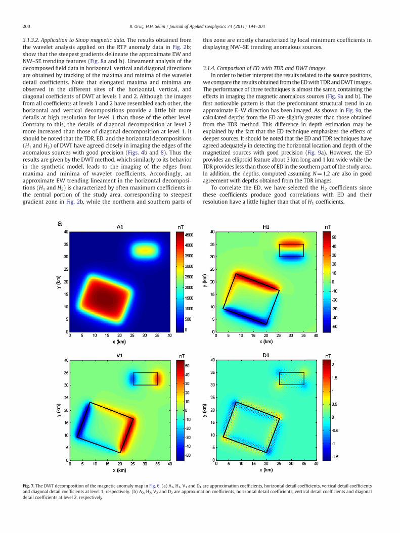
3.1.3.1. Theoretical example. In this section, the robustness of the DWTtechnique used for the edge enhancement is tested with waveletdecomposition of total field anomaly map (Fig. 6) caused by twovertical-sided prisms at a depth to the top of 1.5 km (labeled 1) and 2 km(labeled 2). Fig. 6 shows the theoretical total field anomaly map due tothe two vertical sided prisms in the case of induced magnetization withinclination and declination of 90° and 0°, respectively. The theoreticalmagnetic anomalies of the vertical sided prisms are calculated using theformula given by Rao and Babu (1993) on a regular gridwith a spacing of0.1 km.

Fig. 7a and b shows that the DWT leads to a decomposition ofapproximation coefficients at levels 1 and 2 in four components: theapproximation coefficients (A1 and A2), and the details in threeorientations (horizontal—H1 and H2, vertical—V1 and V2, and diagonal—D1 and D2), respectively. It should be noted that A1 and A2 coefficientswell reflect the theoretical anomalymap in Fig. 6. Thus, one can concludethat theoretical anomaly was successfully decomposed in threeorientations. The resolution of the coefficients (H1, H2, V1, V2, D1 andD2) in three orientations is similar in that their maxima and minima

work well in imaging the edges of the prisms (Fig. 7a and b). It isinteresting to note that the maxima and minima of H1, H2, V1 and V2locate the positions of all the edges of the tilted prismwhile imagingN–Sand E–Wedges of the other one. TheD1 andD2 have imaged the cornersof theprismmodels, as expected.As shown inFig. 7a andb, the advantageof wavelet transform is that it preserves most of the information of theoriginal image in the coarse image. Consequently, we concluded thatimage decomposition process keeps maxima and minima coefficients ofthe decomposed image in the first level and second level of decompo-sition using the Haar wavelets.

200 B. Oruç, H.H. Selim / Journal of Applied Geophysics 74 (2011) 194–204

3.1.3.2. Application to Sinop magnetic data. The results obtained fromthe wavelet analysis applied on the RTP anomaly data in Fig. 2b;show that the steepest gradients delineate the approximate EW andNW–SE trending features (Fig. 8a and b). Lineament analysis of thedecomposed field data in horizontal, vertical and diagonal directionsare obtained by tracking of the maxima and minima of the waveletdetail coefficients. Note that elongated maxima and minima areobserved in the different sites of the horizontal, vertical, anddiagonal coefficients of DWT at levels 1 and 2. Although the imagesfrom all coefficients at levels 1 and 2 have resembled each other, thehorizontal and vertical decompositions provide a little bit moredetails at high resolution for level 1 than those of the other level.Contrary to this, the details of diagonal decomposition at level 2more increased than those of diagonal decomposition at level 1. Itshould be noted that the TDR, ED, and the horizontal decompositions(H1 and H2) of DWT have agreed closely in imaging the edges of theanomalous sources with good precision (Figs. 4b and 8). Thus theresults are given by the DWTmethod, which similarly to its behaviorin the synthetic model, leads to the imaging of the edges frommaxima and minima of wavelet coefficients. Accordingly, anapproximate EW trending lineament in the horizontal decomposi-tions (H1 and H2) is characterized by often maximum coefficients inthe central portion of the study area, corresponding to steepestgradient zone in Fig. 2b, while the northern and southern parts of

Fig. 7. The DWT decomposition of the magnetic anomaly map in Fig. 6. (a) A1, H1, V1 and D1

and diagonal detail coefficients at level 1, respectively. (b) A2, H2, V2 and D2 are approximadetail coefficients at level 2, respectively.

this zone are mostly characterized by local minimum coefficients indisplaying NW–SE trending anomalous sources.

3.1.4. Comparison of ED with TDR and DWT imagesIn order to better interpret the results related to the source positions,

we compare the results obtained from the EDwith TDR andDWT images.The performance of three techniques is almost the same, containing theeffects in imaging the magnetic anomalous sources (Fig. 9a and b). Thefirst noticeable pattern is that the predominant structural trend in anapproximate E–W direction has been imaged. As shown in Fig. 9a, thecalculated depths from the ED are slightly greater than those obtainedfrom the TDR method. This difference in depth estimation may beexplained by the fact that the ED technique emphasizes the effects ofdeeper sources. It should be noted that the ED and TDR techniques haveagreed adequately in detecting the horizontal location and depth of themagnetized sources with good precision (Fig. 9a). However, the EDprovides an ellipsoid feature about 3 km long and 1 km wide while theTDR provides less than those of ED in the southern part of the study area.In addition, the depths, computed assuming N=1.2 are also in goodagreement with depths obtained from the TDR images.

To correlate the ED, we have selected the H2 coefficients sincethese coefficients produce good correlations with ED and theirresolution have a little higher than that of H1 coefficients.

are approximation coefficients, horizontal detail coefficients, vertical detail coefficientstion coefficients, horizontal detail coefficients, vertical detail coefficients and diagonal

Fig. 7. (continued).

201B. Oruç, H.H. Selim / Journal of Applied Geophysics 74 (2011) 194–204

Fig. 9b shows the results of the ED and H2 detail coefficients,correlated well with each other in determining the horizontal locationsof the magnetized sources in the subsurface. Hence it is understood,therefore, that the H2 coefficients are also in good agreement withhorizontal locations obtained from the TDR. A good correspondence isrecognized between the methods in imaging an approximate EWtrending major lineament zone (Fig. 9b). The local lineaments in thesouth and north of this zonewere also traced very well from the ED andH2 coefficients (Fig. 9b).

In conclusion, threemethodshave resembledeachother in detectingthe locations of magnetic lineaments. However, an ellipsoid featureimaged from the TDR in the western part of the study area has not beenconfirmed in DWT image and ED solutions (Fig. 9a and b).

3.2. Delineation of magnetic features

In the study area, the direct correlation of themagnetic pattern withthe superficial geology is difficult to determine because no samplesbelow the bottom of the sea have been obtained. Fig. 10 shows a plot ofthe lineaments identified from a combination of ED, TDR and DWTimages. The interesting observation is all methods have the sameprediction of the edges of the sources. The lineament map summarizesthe most magnetic lineaments of which at least some should representthe edges of themagnetized sourceswithin the Sinop basin in the studyarea. The locationsof features aremappedalong the zero contourof TDR,

the crests of DWT and ED clustering. This map reveals the existence offour small trends except for the main trend. The most prominentmagnetic lineament crossing the entire study area is related to thesouthern edge of the basin (Fig. 10). This is a known boundary faultbordering the southern part of the basin. Within the western of thisdominant trend, two small lineaments, parallel to each other representthe faulting at E–Wdirection. It is clear that these are secondary trendsand close to the dominant trend.

The ellipsoid features may be interpreted as intrabasement units,which are the case for the Sinop basin since such intrusive bodies placewithin the structural framework of the Sinop basin. However, as is wellknown, the pockmarks are craters in the seabed caused by fluids (gasand liquids) erupting and streaming through the sediments. In this case,pockmarks can be interpreted as themorphological expression of gas orleakage from active hydrocarbon system. Fichler et al. (2005) haveintroduced that the pockmarks occur near a major fault, and highfrequency magnetic anomalies at such locations can be explained bydeposition of sediments with contrasting magnetic susceptibilities.Çiftçi et al. (2003) have presented the pockmarks were formed inexpulsive nature in tectonically relaxed zones. Thus they have alsointroduced that North Anatolian Fault has had a significant effect on thetectonic and overpressure conditions in the area, and could modify theoverpressure conditions of the shelf cyclically.

The above discussion provides a more detailed investigation for atreatment of the subsurface below the sea bottom, such as acoustic

Fig. 8. The discrete wavelet decomposition of the RTP data in Fig. 2b at levels 1 and 2. (a) A1, H1, V1 and D1 are approximation coefficients, horizontal detail coefficients, verticaldetail coefficients and diagonal detail coefficients at level 1, respectively. (b) A2, H2, V2 and D2 are approximation coefficients, horizontal detail coefficients, vertical detailcoefficients and diagonal detail coefficients at level 2, respectively.

202 B. Oruç, H.H. Selim / Journal of Applied Geophysics 74 (2011) 194–204

surveys. The improvement in resolution from the proposed techniquesprovides a good visualization of outlines of geologic features. On thebasis of Fig. 10 shows a schematic representation of the lineament mapobtained from joint modeling.

4. Conclusions

Our main contribution in this study has been to present theeffectiveness of the TDR, ED and DWT from RTP anomaly data for the

Fig. 9. Comparison of ED with (a) zero contour of TDR images, and (b) maxima andminima of DWT images. Note that the source locations from ED, TDR and DWTtechniques produce good correlations.

203B. Oruç, H.H. Selim / Journal of Applied Geophysics 74 (2011) 194–204

interpretation of magnetic data. The results coming out of this studyfacilitate the identification of new features as well as the mapping ofknown main trend that represents the southern edge of a small part ofSinop basin. Thus these results allow the basement faulting distribution,

Fig. 10. Map showing structural elements of the study area based on integration of theresults obtained from the TDR, ED and DWT.

producing a structural map showing the magnetic lineaments for thesurvey area.

A particular interest for mapping in the horizontal dimension islocating lateralmagnetization contrasts, equatedwith geologic contacts.We find that the three methods considered are redundant, givingpractically identical results for imaging the edges of the anomaloussources. The TDR have clear indications of utility to infer the location ofthe boundaries of magnetized lithologies since the analysis of TDR isonly based on the contours of three angles of 0,−π/4 and+π/4 radians.The ED and DWT almost confirmed the results from the TDR under theassumption that the edges of anomalous sources are caused by verticalcontacts. All techniques show the presence of a lineament in the EWtrending that separates northern and southern basement blocks in thesouth of Sinop basin. This lineament bordering the south of Sinop basinlikely controls theNE–SW trending features in the study area. Accordingto the results, it is concluded that the study area represents a small partof the Black sea area that has been affected by tectonic movementsduring its geological history. The linear subsurface features and ellipsoiddepressions (pockmarks) are attractive for delineating oil and gas traps.It is possible to conclude that the potential new oil and gas reservoirs inthe study area of the Sinop basin will be likely associated with thesefeatures. These features are most likely representing an intrusion orpockmarks associated with the extensional graben system. In conclu-sion, attention should be paid to this fact in further analyses ofgeophysical and geological data. Thus, further research is needed toexplain theway the localmagnetic anomalies are related to both oil andgas fields in the study area.

Acknowledgments

The authors are thankful to Turkish Navy Department of Navigation,Hydrography andOceanography for supplying geophysical data. Thanksare also due to anonymous reviewers whose careful reviews improvedthis work.

References

Albora, A.M., Hisarlı, Z.M., Uçan, O.N., 2004. Application of wavelet transform tomagnetic data due to ruins of the Hittite, civilization in Turkey. Pure and AppliedGeophysics 161, 907–930.

Blakely, R.J., Simpson, R.W., 1986. Approximating edges of source bodies frommagneticand gravity anomalies. Geophysics 51, 1494–1498.

Çiftçi, G., Dondurur, D., Ergün, M., 2003. Deep and shallow structures of largepockmarks in the Turkish shelf, Eastern Black Sea. Geo-Marine Letters 23, 311–322.

Cooper, G.R.J., Cowan, D.R., 2006. Enhancing potential field data using filters based onthe local phase. Computers and Geosciences 32, 1585–1591.

Cordell, L., Grauch, V.J.S., 1985. Mapping basement magnetization zones from aeromag-netic data in the San Juan basin, New Mexico. In: Hinzc, W.J. (Ed.), The Utility ofRegional Gravity and Magnetic Anomaly Maps: Soc. Expl. Geophys. , pp. 181–197.

Daubechies, I., 1992. Ten Lectures on Wavelets. Vol. 61 of CBMS-NSF RegionalConference Series in Applied Mathematics. SIAM Publications, Philadelphia.

Dondurur, D., Çiftçi, G., 2008. Anomalous strong reflections on high resolution seismic datafrom theTurkish Shelf of theEasternBlack Sea:possible indicatorsof shallowhydrogensulphide-rich gas hydrate layers. Turkish Journal of Earth Sciences 18, 299–313.

Fedi, M., Quarta, T., 1998. Wavelet analysis for the regional–residual and localseparation of the potential field anomalies. Geophysical Prospecting 46, 507–525.

Fichler, C., Henriksen, S., Rueslaatten, H., Hovland, M., 2005. North sea Quaternarymorphology from seismic and magnetic data: indications for gas hydrates duringglaciation. Petroleum Geosciences 11, 331–337.

Foufoula-Georgiou, E., Kumar, P. (Eds.), 1994.Wavelets in Geophysics. Acad. Press, NewYork. 235 pp.

Gökaşan, E., 1996. Anadolu'nun karadeniz kıyılarının neotektoniğine bir yaklaşım.Yerbilimleri 29, 99–109.

Gunn, P.J., 1975. Linear transformations of gravity and magnetic fields. GeophysicalProspecting 23, 300–312.

Hornby, P., Boschetti, F., Horovitz, F.G., 1999. Analysis of potential field data in thewavelet domain. Geophysical Journal International 137, 175–196.

Hsu, S.-K., 2002. Imaging magnetic sources using Euler's equation. GeophysicalProspecting 50, 15–25.

Kazmin, V.G., Schreider, A.A., Bulychev, A.A., 2000. Early stages of evolution of theBlack Sea. In: Bozkurt, E., Winchester, J.A., Piper, J.D.A. (Eds.), Tectonics andMagmatism in Turkey and the Surrounding Area: Geol. Soc. Lond. Spec. Publ., 173,pp. 235–249.

Keating, P., Pilkington, M., 2004. Euler deconvolution of the analytic signal and itsapplication to magnetic interpretation. Geophysical Prospecting 52, 165–182.

204 B. Oruç, H.H. Selim / Journal of Applied Geophysics 74 (2011) 194–204

Li, Y., Oldenburg, D.W., 2003. Fast inversion of large scale magnetic data using wavelettransforms and a logarithmic barrier method. Geophysical Journal International152, 251–265.

Mallat, S., 1989. A Theory for multi-resolution signal decomposition the waveletrepresentation. IEEE Trans. Pattern Anal. Mach. Intell. 31, 679–693.

Miller, H.G., Singh, V., 1994. Potential field tilt—a new concept for location of potentialfield sources. Journal of Applied Geophysics 32, 213–217.

Moreau, F., Gibert, D., Holschneider, M., Saracco, G., 1997. Wavelet analysis of potentialfields. Inverse Problems 13 (1), 165–178.

Moreau, F., Gibert, D., Holschneider, M., Saracco, G., 1999. Identification of sources ofpotential fields with the continuous wavelet transform: basic theory. Journal ofGeophysical Research 104, 5003–5013.

Özhan, G., 2004. Sinop açıklarında jeolojik ve aktif çizgisel bulgular. Kıyı ve DenizJeolojisi Sempozyumu. 13–15 Eylül 2004, İstanbul, p. 21.

Rangin, C., Bader, A.G., Pascal, G., Ecevitoğlu, B., Görür, N., 2002. Deep structure of themid Black Sea high (offshore Turkey) imaged by multi-channel seismic survey(BLACKSIS Cruise). Marine Geology 182, 265–278.

Rao, D.B., Babu, N.R., 1993. A FORTRAN-77 computer program for three-dimensionalinversion of magnetic anomalies resulting from multiple prismatic bodies.Computers and Geosciences 19, 781–801.

Ravat, D., 1996. Analysis of the Euler method and its applicability in environmentalinvestigations. Journal of Environmental and Engineering Geophysics 1, 229–238.

Reid, A.B., Alsop, J.M., Grander,H.,Millet, A.J., Somerton, I.W., 1990.Magnetic interpretationin three dimensions using Euler deconvolution. Geophysics 55, 80–91.

Ridsdill-Smith, T.A., Dentith, M.C., 1999. The wavelet transform in aeromagneticprocessing. Geophysics 64, 1003–1013.

Robinson, A.G., Rudat, J.H., Banks, C.J., Wiles, R.L.F., 1996. Petroleum geology of the BlackSea. Marine and Petroleum Geology 13, 195–223.

Salem, A., Williams, S., Fairhead, J.D., Ravat, D.J., Smith, R., 2007. Tilt-depth method: asimple depth estimation method using first-order magnetic derivatives. TheLeading Edge 26, 1502–1505.

Salem, A., Williams, S., Fairhead, J.D., Smith, R., Ravat, D.J., 2008. Interpretation ofmagnetic data using tilt-angle derivatives. Geophysics 73, P.L1–P.L10.

Schmidt, P.W., 2006. Inversion using Euler deconvolution of the magnetic gradienttensor. ASEG Extended Abstracts 1, 1–3.

Stavrev, P.Y., 1997. Euler deconvolution using differential similarity transformations ofgravity or magnetic anomalies. Geophysical Prospecting 45, 207–246.

Thompson, D.T., 1982. EULDPH—a technique for making computer-assisted depthestimates from magnetic data. Geophysics 47, 31–37.

Varol, 2004. Stable isotopes of mollusk shells in environmental interpretations; anexample from Sinop miocene succession (northern Turkey). Mineral ResearchExploration Bulletin 128, 49–60.

Verduzco, B., Fairhead, J.D., Green, C.M., Mackenzie, C., 2004. New insights intomagnetic derivatives for structural mapping. The Leading Edge 23, 116–119.

Wijns, C.C.P., Perez, C., Kowalczyk, P., 2005. Thetamap: edge detection inmagnetic data.Geophysics 70, L39–L43.

Yılmaz, Y., Tüysüz, O., Yiğitbaş, E., Genç, C., Şengör, A.M.C., 1997. Geology and tectonicevolution of Pontides. In: Robinson, A.G. (Ed.), Regional and Petroleum Geology ofBlack Sea and Surrounding Region: AAPG Memoir, 68, pp. 183–226.