journal of geophysical research, vol. 88, no. …lyutikov/liter/jupiterbelt.pdf · journal of...

JOURNAL OF GEOPHYSICAL RESEARCH, VOL. 88, NO. A9, PAGES 6889-6903, SEPTEMBER 1, 1983

Charged Particle Distributions in Jupiter's Magnetosphere NEIL DIVINE AND H. B. GARRETT

Jet Propulsion Laboratory, California Institute of Technology

A compact, quantitative model of the distribution of charged particles between 1 eV and several MeV in the Jovian magnetosphere is presented. The model is based primarily on in situ data returned by experiments on the Pioneer and Voyager spacecraft, supplemented where necessary by earth-based observations and theoretical considerations. Thermal plasma parameters, notably convection speed, number density, and characteristic energy, are specified as functions of position for electrons and several ion species (H +, O +, O + +, S +, S + +, S + + +, and Na +). At intermediate energy the electron and proton populations are modeled using kappa distributions, which join smoothly onto the radiation belt spectra at high energies (E > 100 keV). At these energies the radiation belt intensity spectra include angular distributions for energetic electrons inside 16 Rj and protons inside 12 Rj. Major features of the magnetic field, thermal plasma, and trapped particle distributions are modeled, such as ring and satellite absorption signatures and corotational flow within the Io plasma torus and the current disk. Within each plasma region the model results are compared with observed spectra, showing that the model represents the data typically to within a factor of 2 +- • except where time variations, neglected in the model, are known to be significant. Several practical applications of the model to spacecraft near Jupiter are illustrated with sample results from radiation analyses and electrostatic charging calculations.

INTRODUCTION

Jupiter has been known to have a magnetosphere since about 1960 when, in analogy with early spacecraft observations of the earth's radiation belts, it was realized that the Jovian UHF radio emissions could be interpreted in terms of trapped energetic electrons [Drake and Hvatum, 1959]. Early speculation by Brice [Brice and Ioannidis, 1970; Ioannidis and Brice, 1971] and others attempted to draw parallels between this hypothesized Jovian magnetosphere and the then current ideas of the earth's magnetosphere. In order to assess the potential hazard to the Pioneer 10 and 11 spacecraft, crude numerical models of the energetic electrons and protons were developed based on these specula- tions and the early radio observations (see summary by Beck [1972]; also later papers by Coroniti [1974] and Kennel and Coroniti [1975]). The successful encounters of the Pioneer spacecraft with the Jovian magnetosphere gave rise to a number of quantitative models describing various aspects of the Jovian magnetosphere (see books by Formisano [1975] and Gehrels [1976]). In particular, magnetic field models by Smith et al. [1976] and Acuna and Ness [1976a, b] began to delineate the substantial differences that exist between the Jovian and terrestrial magnetospheres. Pronounced wave- like variations in the high-energy particle fluxes led Van Allen et al. [1974] to propose that the Jovian magnetosphere was distorted into a thin disc, the so-called magnetodisc theory. It was further suggested that this thin disc was populated by a cold plasma consisting of heavy ions originat- ing from Io [Hill and Michel, 1976; Neugebauer and Eviatar, 1976] (see also review by Goertz and Thomsen [1979]). Models by Hill [1976, 1979], Carbary et al. [1976], and Hill and Carbary [1978] predicted the nature and rate of the outflow of this cold plasma. The so-called" magnetic anomaly" model of Dessler and Vasyliunas [1979] [see also Vasy- liunas and Dessler, 1981], which predicts that the asymme-

This paper is not subject to U.S. copyright. Published in 1983 by the American Geophysical Union. Paper number 3A0932.

tries present in the Jovian magnetic field significantly influence the entire magnetosphere, was also developed in this period. The passage of the Voyager 1 and 2 spacecraft, while failing to distinguish between the magnetic anomaly and magnetodisc models, further refined the particle and field observations. Subsequently, theoretical models [e.g., Connerhey et al., 1981; $iscoe and Summers, 1981; Richard- son and $iscoe, 1981; Carbary, 1980; etc.] have further helped to interpret the observations and have led to the beginning of the development of Jovian magnetospheric models capable of being used to make practical predictions about the environment around Jupiter. The objective of this paper is to incorporate in situ measurements of the Pioneer and Voyager spacecraft, earth-based observations, and con- cepts advanced by these theoretical models into what is the first compact, comprehensive numerical model of the Jovian magnetosphere. Such a model is currently needed to carry out a number of practical calculations associated with the effects of the Jovian environment: several examples of which will be presented.

Table 1 summarizes the spacecraft instruments, the data types, and the references from which the model has been derived. Table 2 lists the various partially independent components of the model. The following sections discuss the coordinate system and the magnetic field model assumptions, the development and quantitative description of each of these components, and the comparisons between the data and observations. The final section presents examples of several practical applications of the model.

THœ JOVIAN COORDINATE SYSTEM

In deriving the model, several assumptions regarding the proper coordinate system to employ were necessary. In the present model the independent variables used to define position for the magnetic field and charged particles are jovicentric distance r (commonly in meters or Rs), latitude X (deg or rad), longitude l (deg in System III (1965)), distance z = r sin X from the rotational equatorial plane (m or R j), and distance R = r cos h from the rotation axis (rn or R j). The value of the Jovian equatorial radius is assumed to be 1 Rj =

6889

6890 DIVINE AND GARRETT: THE MAGNETOSPHERE OF JUPITER

TABLE 1. Data Sources for Jupiter Charged Particle Models

Instrument Data Type References

Helium vector magnetometer (HVM)

Flux gate magnetometer (FGM)

Plasma analyzer (PA)

Geiger tube telescope (GTT)

Trapped radiation detector (TRD)

Low-energy telescope (LET)

Electron current detector (ECD)

Fission cell (F 1)

Flux gate magnetometer (MAG)

Planetary radio astronomy (PRA)

Plasma wave (PWS)

Plasma science (PLS)

Low-energy charged particle (LECP)

Cosmic ray telescope (CRT)

Radio telescopes

Pioneers 10 and 11 vector magnetic field

vector magnetic field

electrons and protons, 0.1 to 4.8 keV

electrons >0.06, 0.55, 5, 21, 31 MeV

protons 0.61-3.41 MeV electrons >0.16, 0.26, 0.46, 5,

8, 12, 35 MeV protons >80 MeV protons 1.2-2.15 and 14.8-

21.2 MeV

electrons >3.4 MeV

protons >35 MeV

Voyagers 1 and 2 vector magnetic field

electric vector, 1.2 kHz to 40.5 MHz

10 Hz to 56 kHz

electrons 10-6000 eV ions 10-6000 V

electrons >15 keV ions >30 keV electrons 3-110 MeV ions 1-500 MeV/nucleon

Earth UHF intensity and polariza-

tion

Smith et al. [1976]

Acuna and Ness [1976a, b]

Frank et al. [1976]

Van Allen et al. [1974, 1975], Van Allen [1976], and Baker and Van Allen [1977]

Fillius and Mcllwain [1974], Fillius et al. [1975], and Fil- lius [ 1976]

Trainor et al. [1974, 1975] and McDonald and Trainor [1976]

Simpson et al. [1974, 1975]

Simpson and McKibben [1976]

Ness et al. [1979a, b]

Warwick et al. [1979a, b] and Birmingham et al. [1981]

Scarlet al. [1979] and Gur- nett et al. [1979]

Bridge et al. [1979a, b], Ba- genal and Sullivan [1981], and Scudder et al. [1981]

Krimigis et al. [1979a, b, 1981]

Vogt et al. [1979a, b]

Berge and Gulkis [1976] and dePater and Dames [1979]

7.14 x 107 m. The common angular speed of rotation of Jupiter's internal magnetic field and of a meridian of constant longitude I in System III (1965) coordinates is assumed to be •o = 870.536 deg/d • 12.6 km/s Rj. In this system, l, the longitude, increases westward (opposite to the azimuthal angle in a system of spherical coordinates). Conversions to inertial and other coordinate systems may be derived from Seidelmann and Divine [ 1977]. Where logarithms are used in the model, base 10 is intended.

MAGNETIC FIELD MODEL

Of the four encounters with Jupiter the retrograde, highly inclined, small perijove trajectory flown by Pioneer 11 has been the most useful for modeling the moments of Jupiter's internal magnetic field. Therefore the detailed, 15-coefficient spherical harmonic model 04 derived from the flux gate magnetometer on Pioneer 11 [Acuna and Ness, 1976a, b] was used in deriving the model presented here. In this model the dipole moment will be assumed to have the value M - 1.535 x 1027 m 2 A = 4.218 G Rj 3, and for each field line the magnetic shell parameter L has the constant value

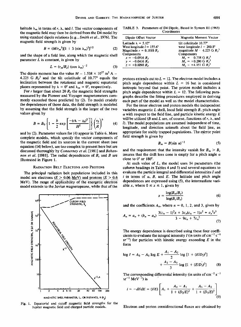
L = (M/Be) 1/3 Rj -1 (1) where Be represents the minimum field strength along the line. Among all field lines having the same value of L, the smallest field strength for which Jupiter's atmosphere (equatorial radius 1 R j, flattening 0.065) is encountered represents an upper cutoff field strength Bc for stable charged particle

trajectories. The 04 model has been used to calculate Bc as a function of L (the upper dashed curve in Figure 1) and to analyze the energetic charged particle data in the development of the numerical models. Although the 04 magnetic field model was used in deriving the model parameters, the much simpler offset tilted dipole model D4 derived from the Pioneer helium vector magnetometer data [Smith et al., 1976] provides adequate accuracy for evaluating model parameters for many applications. The parameter values for this model are presented in Table 3. The nearly equatorial offset of about 0.1 Rj suggests that L - 1.1 represents the smallest accessible value of L for the trapped particles (the 04 model yields minimum L = 1.089). The transformation of coordinates in Table 3 allows derivation of distance rm and

TABLE 2. Components of the Jupiter Charged Particle Model

Model Component Particles and Energy

Ranges Dipole magnetic field Exterior magnetic field Radiation belts

Intermediate energy

Inner plasmasphere Cool torus Warm toms Inner disc Outer disc

electrons > 0.06 MeV protons > 0.6 MeV electrons •> 1 keV protons •> 1 keV

thermal electrons < 1 keV thermal ions < 1 keV

DIVINE AND GARRETT: THE MAGNETOSPHERE OF JUPITER 6891

latitude hm in terms of r, h, and 1. The vector components of the magnetic field may then be derived from the D4 model by using standard dipole relations [e.g., Smith et al., 1976]. The magnetic field strength is given by

B = (M/rm3)[1 + 3 (sin hm)2] 1/2 (2) and the shape of a field line, along which the magnetic shell parameter L is constant, is given by

L = (rm/aj) (cos •m) -2 (3) The dipole moment has the value M = 1.538 x 1027 m 2 A = 4.225 G Rj 3 and the tilt colatitude of 10.77 ø equals the inclination between the rotational and magnetic equatorial planes represented by h = 0 ø and krn = 0 ø, respectively.

For r larger than about 20 Rj the magnetic field strengths measured by the Pioneer and Voyager magnetometers commonly exceeded those predicted by (2). To model crudely the dependences of those data, the field strength is modeled by assuming that the field strength is the larger of the two values given by

B=B0{1-bexp[-(rh-zø)2 and by (2). Parameter values for (4) appear in Table 6. More complete models, which specify the vector components of the magnetic field and its sources in the current sheet (see equation (14) below), are too complex tO present here but are discussed thoroughly by Connerney et al. [1981] and Behan- non et al. [1981]. The radial dependences of Bc and B are illustrated in Figure 1.

RADIATION BELT ELECTONS AND PROTONS

The principal radiation belt populations included in this model are electrons (E > 0.06 MeV) and protons (E > 0.6 MeV). The range of aPpl•ca•il-ity of the energetic electron model extends to the Jovian magnetopause, while that of the

,06[

104

103

100

/ c UTOFF FI ELD

.---._.. •// STRENGTH• B c -

_

--

2 4 6 8 10 20 40 60 100 200

MAGNETIC SHELL PARAMETER, L, OR DISTANCE, R (R j) Fig. 1. Equatorial and cutoff magnetic field strengths œor the

Jupiter magnetic field and charged particle models.

TABLE 3. Parameters of D4 Dipole, Based in System III (1965) Coordinates

Dipole Offset Vector Magnetic Moment Vector Latitude h = 5.12 ø West longitude I = 155.6 ø Magnitude r = 0.1010 Rj Components

x = -0.0916 Rj y = -0.0416 R• z = +0.0090 R•

tilt colatitude 10.77 ø west longitude I = 200.8 ø magnitude M - 4.225 G Rj 3 Components

Mx = -0.738 G Rj 3 My = +0.280 G Rj 3 M.. = +4.!51 G Rj 3

protons extends out to L = 12. The electron model includes a pitch angle dependence within L -- 16 but is considered isotropic beyond that point. The proton model includes a pitch angle dependence within L - 12. The following para- graphs describe the fitting procedures employed in deriving each part of the model as well as the model characteristics.

For the inner electron and proton models the independent variables magnetic L shell, local field strength B, pitch angle a with respect to the field line, and particle kinetic energy E will be utilized (B and L are, of course, functions of r, •, and l). The model populations are assumed independent of time, longitude, and direction azimuth about the field line, as appropriate for stably trapped populations. The mirror point

,

field strength is given by

Bm= B(sin a) -2 (5) and the requirement that the intensity vanish for Bm • Bc insures that the drift loss cone is empty for a pitch angle a close to 0 ø or 180 ø.

At each value of L, the model uses 14 parameters (the column headings in Tables 4 and 5) and several equations to evaluate the particle integral and differential intensities I and i in terms of a, B, and E. The latitude and pitch angle dependences are expressed using (5), the intermediate variable x, where 0 -< x -< 1, given by

log(Bin/Be) x = (6)

log(Bc/Be)

and the coefficients An, where n = 0, 1, 2, and 3, given by

3(Cn- 1)2X + 3Cn(Cn -- 1)X 2 + Cn2X 3 An = an + (bn - an) 3 - 9Cn + 7Cn 2

(7)

The energy dependence is described using these four coefficients to evaluate the integral intensity I (in units of cm -2 s- l sr -1) for particles with kinetic energy exceeding E in the form

A1 - A2 logI=A0-AllogE+•log[1 + (E/D2) 2]

2 A2 - A3 + • log [1 + (E/D}) 3] (8)

3

The corresponding differential intensity (in units of cm -2 s-l sr -1 MeV -1) is •:

[ A2-A1 A3-A2 ] i = - dI/dE = (I/E) A l q- q- • 1 + (D2/E) 2 1 + (D3/E) 3

(9)

Electron and proton omnidirectional fluxes are obtained by


TABLE 4. Parameter Values for Jupiter Trapped Electron Model

L ao a• a2 a3 bo b• b2 b3 Co c• c2 c• D2 D3 1.089 6.06 0.00 0.00 4.70 6106 0.00 0.00 4.70 0.00 0.00 0.81 0.50 2.0 30.0 1.55 6.90 0.30 4.30 1.75 7.•34 0.57 3.98 1.90 7.00 0.47 4.38 6.51 5.42 0.83 2.00 7.36 0.75 3.65 6.26 4.76 0.68 2.10 7,29 0.69 3.41 6.33 4.79 0.70 2.40 7.31 0.72 0.67 4. i5 5191 5.21 0.58 0.14 0.18 0.7 26.0 2.60 7.33 0.96 0.69 4.24 5.79 4.85 0.55 0.06 0.00 2.80 7.39 0.76 0.59 2.65 5.86 6.09 0.56 0.36 0.35 0.2 22.0 2.85 7.44 0.80 0.60 2.65 5.80 6.09 0.56 0.37 0.35 3.2 7.00 1.32 0.53 2.65 5.89 6.09 0.49 0.40 0.35 3.6 6.91 1.37 0.51 3.51 5.75 6.70 0.58 0.49 0.35 5.2 6.21 1.70 0.48 4.93 5.80 0.34 4.28 0.56 0.00 0.50 6.2 6.37 1.33 0.00 2.27 6.33 1.66 3.07 0.56 0.13 0.40 1.0 10.0 7.2 6.39 1.07 0.02 3.02 6.12 1.82 3.56 0.32 0.06 0.40 9.0 6.60 0.65 0.54 3.60 5.63 0.65 2.07 2.00 0.00 0.59 0.47

10.5 7.23 0.59 1.95 2.23 5.73 0.93 2.71 0.55 0.00 0.62 0.56 11.0 7.07 0.92 2.00 2.00 5.56 0.82 2.82 0.56 0.57 0.47 0.00 12.0 6.76 0.95 2.13 5.00 1.20 2.99 0.58 0.26 0.37 14.0 6.67 0.20 2.90 3.34 2.86 1.01 0.62 0.65 0.00 16.0 4.44 0.89 0.90 5.86 0.76 7.95 0.00 0.26 0.70

Where an entry is absent, the value immediately above is to be used (also in Table 5).

integration

f0 •/2 J = 4•r /(sin (10)

In (7)-(10), E, D2, and D3 are energies (in MeV), the values for A0, a0, and b0 reflect the units for I and i,•while all other quantities are dimensionless parameters which represent the dependences on energy and (through x) on latitude and pitch angle.

The spectra represented by (5)-(9) are approximate power laws, where transitions between the exponents A•, A2"and

,

A3 occur near the energies D2 and D3. The pitch angle anisotropy and latitude variations are represented by the transitions of the coefficients A0 through A3 from the values a0 through a3 for x = (1 (at the magnetic equator) to the values b0 through b3 for x = 1 (at the cutoff mirror point field); the steepness of the transition is controlled by the parameters Co through c3. Except as fitting parameters to match the data, no major physical significance has been inferred from the values of these coefficients.

Values for the constants in (7)-(10) (see Tables 4 and 5) were obtained by minimizing the weighted root mean square residual in the logarithm of the ratios of the model-predicted

TABLE 5. Parameter Values for Jupiter Trapped Proton Model ß

L ao a• a2 a3 bo b• b2 b3 Co Cl c2 c3 D2 D3 1.089 3.59 0.44 0.27 3.87 3.59 0.44 0.27 3.87 0.00 0.00 0.00 0.00 1.2 30.0 1.60 7.10 0.00 0.13 3.54 1.75 6.65 0.06 0.11 3.87 1.80 6.47 0.04 0.18 4.15 4.68 0.11 0.09 4.15 1.85 6.09 0.02 0.30 4.09 5.28 0.01 0.05 4.09 1.9 6.33 0.00 0.21 3.58 4.96 0.00 0.25 3.58 2.0 7.03 0.11 3.29 4.49 0.24 3.29 2.1 7.09 0.13 3.54 4.52 0.15 3.54 2.2 6.73 0.10 0.08 3.29 4.44 0.08 0.22 3.29 2.3 6.51 0.01 0.05 2.95 3.57 1.29 0.22 2.95 2.4 5.64 0.97 0.19 3.01 4.44 0.02 0.46 3.01 2.5 5.25 1.98 0.21 3.03 4.59 0.00 0.06 4.07 0.10 0.15 0.15 0.10 2.6 4.70 2.98 0.01 2.77 5.08 0.00 0.00 4.44 0.20 0.30 0.30 0.20 2.7 5.72 2.77 0.00 3.27 4.67 0.15 3.89 0.30 0.45 0.45 0.30 2.8 6.27 3.56 0.00 3.28 4.58 0.42 3.72 0.40 0.57 0.55 0.41 2.85 7.08 0.00 0.90 6.00 4.37 0.58 3.00 0.40 0.57 0.55 0.41 3.0 7.29 0.08 2.14 4.58 0.40 2.76 0.45 0.64 0.54 0.45 5.6 3.2 7.17 0.52 0.73 4.88 0.00 2.70 0.49 0.00 0.54 0.25 5.9 3.4 7.07 0.84 0.00 4.89 2.99 0.47 0.37 0.00 0.33 4.0 3.6 7.09 0.55 0.55 4.87 3.16 0.48 0.01 0.55 0.42 3.4 4.5 6.70 0.70 0.98 4.05 1.17 2.00 0.51 0.61 0.41 0.30 1.0 5.4 5.89 0.89 0.90 3.89 1.13 0.53 0.44 0.54 0.25 3.6 5.8 5.20 1.66 0.52 3.22 4.77 0.09 2.02 0.44 0.61 0.54 0.21 1.2 6.2 6.00 1.98 0.52 3.21 3.11 0.00 2.06 0.03 0.64 0.50 0.14 2.6 6.6 6.92 3.13 0.66 5.53 4.06 2.36 2.58 0.22 0.00 0.00 0.09 4.0 7.0 7.10 3.63 0.38 5.96 5.11 0.61 1.72 2.67 0.49 0.75 0.50 9.0 6.74 2.61 1.69 6.00 4.32 3.92 0.00 2.40 0.65 2.99 0.86 0.00

12.0 5.58 1.30 3.21 6.00 4.23 3.33 3.39 2.40 0.61 0.00 0.56 0.00

See note to Table 4. ,•


count rates to the count rates observed from several detectors at the L values listed in Tables 4 and 5. These detectors, having the approximate energy ranges or thresholds shown in Table 1 (column 2), were part of four experiment packages flown on Pioneer 10 and 11. The dependence on the magnetic shell parameter is then achieved by allowing each of the 14 parameters an, bn, Cn, D2, and D3 to be linear in L between the entries on adjacent rows in Tables 4 and 5. For most of the observations, detector response functions, corrected count rates, and suggested weights were obtained directly from the experimenters (see Table 1). A later section of the paper will discuss improvements in the fits which were derived by matching the model predictions to UHF radio observations from earth.

All the particle count rate data available from the Pioneer 10 and 11 references listed in Table 1, plus some data obtained directly from the experiment teams, were used in the model parameter evaluations. Exceptions to this general rule were made for data outside the L range of the model and for data superseded by later expert reintepretation for example, the replacement of raw count rates by those corrected for instrument dead time or saturation. Further, unit weight was assigned to each count rate separately except in those few cases where noise, saturation, or other irregularities were judged sufficient to •arrant a lesser weight. The root mean square residuals in the logarithm of the count rate ratios (model to observed) vary modestly with L and particle kind but are commonly in the range 0.2-0.3 at L < 12 and ->0.4 at L >- 12 for electrons (similarly for protons, with the increase occurring for L -> 9). Thus in most regions the formal consistency of the data set is comparable to the overall flux uncertainty of 2 -+] suggested by several of the experiment teams. Additionally, the proton model inter-

I I I I I I I I I I I I I I I• 10 9 -

'T,,, lO 8-

v• •o z- • 10 6-- - O

I I I

1 3 4 5 6 7 8 9 10 11 12 13 14 15 MAGNETIC SHELL PARAMETER, L (R j)

A 108 [ T• T •"' 1071'

-- lO 6

z o • ,• 1 Z

•o 4

-- I I I bt L=2 I__' • ' i ' I c

107•= 2 - - 6.2 •

i i i lO.5] I , I , I , I 0.1 1.0 10 0 20 40 60

ENERGY, E (MeV) MAGNETIC LATITUDE, X m (deg)

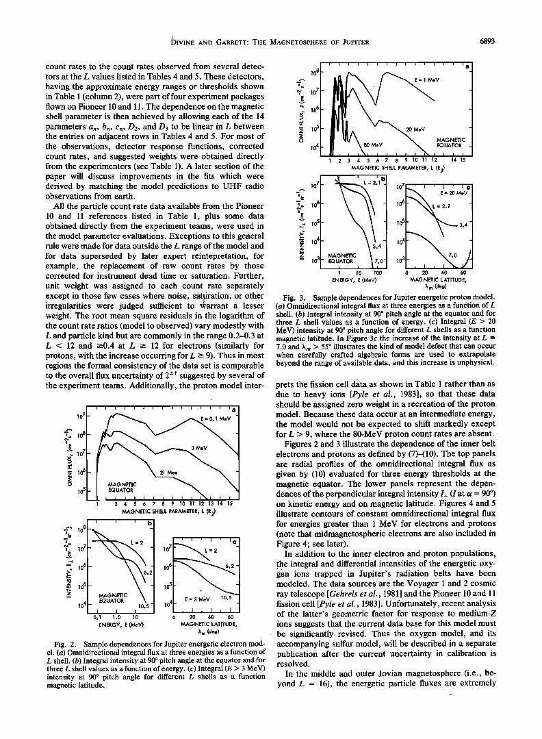
Fig. 2. Sample dependences for Jupiter energetic electron model. (a) Omnidirectional integral flux at three energies as a function of L shell. (b) Integral intensity at 90 ø pitch angle at the equator and for three L shell values as a function of energy. (c) Integral (E > 3 MeV) intensity at 90 ø pitch angle for different L shells as a function magnetic latitude.

I i i i I i i I I I i I I I i a lost t,,_ • • - 5-' E=i MeV

- i - • 106 I'!1^ v -

o / i• •v X _. • MAGNETIC

[ i I I I •1 I I I i I I% I I I I 1 2 3 4 5 6 7 8 9 10 11 12 14 15

MAGNETIC SHELL P•ETEE, L (R j)

10 7 =2. •' I ' I ' • C

• 3. - M _ 7,0 .

1 10 1 • 0 20 40 60 ENERGY• E (MeV) MAGNETIC LATITUDE•

Xm (deg)

Fig. 3. Sample dependences for Jupiter energetic proton model. (a) Omnidirectional integral flux at three energies as a function of L shell. (b) Integral intensity at 90 ø pitch angle at the equator and for three L shell values as a function of energy. (c) Integral (E > 20 MeV) intensity at 90 ø pitch angle for different L shells as a function magnetic latitude. In Figure 3c the increase of the intensity at L = 7.0 and X• > 55 ø illustrates the kind of model defect that can occur when carefully crafted algebraic forms are used to extrapolate beyond the range of available data, and this increase is unphysical.

prets the fission cell data as shown in Table 1 rather than as due to heavy ions [Pyle et al., 1983], so that these data should be assigned zero weight in a recreation of the proton model. Because these data occur at an intermediate energy, the model would not be expected to shift markedly except for L > 9, where the 80-MeV proton count rates are absent.

Figures 2 and 3 illustrate the dependence of the inner belt electrons and protons as defined by (7)-(10). The top panels are radial profiles of the omnidirectional integral flux as given by (10) evaluated for three energy thresholds at the magnetic equator. The lower panels represent the dependences of the perpendicular integral intensity L_ (I at a = 90 ̧) on kinetic energy and on magnetic latitude. Figures 4 and 5 illustrate contours of constant omnidirectional integral flux for energies greater than 1 MeV for electrons and protons (note that midmagnetospheric electrons are also included in Figure 4; see later).

In addition to the inner electron and proton populations, the integral and differential intensities of the energetic oxy- g•en ions trapped in jupiter, s.•radiation belts have been modeled. The data sources are the Voyager 1 and 2 cosmic ray telescope [Gehrels et al., 1981] and the Pioneer 10 and 11 fission cell [Pyle et al., 1983]. Unfortunately, recent analysis of the latter's geometric factor for response to medium-Z ions suggests that the current data base for this model must be significantly revised. Thus the oxygen model, and its accompanying sulfur model, will be described in a separate publication after the current uncertainty in calibration is resolved.

In the middle and outer Jovian magnetosphere (i.e., beyond L = 16), the energetic particle fluxes are extremely

_


-8 • __ 104 J -10] • • i

0 2 4 6 8 10 12 14 16 i8 20

Rj Fig. 4. Contours of equal omnidirectional integral (E > i MeV)

electron flux for a meridional cross section at I = 110øW. The horizontal axis represents distance along the rotational equator.

time dependent and are, as a result, difficult to model. However, to estimate adequately radiation effects in the Jovian environment, a Simple, isotropic formula for the energetic electron fluxes, based on Pioneer 10 and 11 observations,. has been included in the model for completeness. This formulation assumes that the peak equatorial fluxes can be described by a function of the form

log J0 = f(t) - 2.2 log r - 0.7 log (0.03E + E3/r) (11) Here the electron kinetic energy E has units MeV, r has units

-2 R j, and the omnidirectional integral flux J has units of cm s -•. The term f(t), which specifies the time dependence, is assumed to have an average value of 7.43. The maximum value given by (11) is assumed to occur along a disk surface at a height z0 (in Rj) above the Jovian equatorial plane given by (Table 6; see also Carbary [1980])

(7r- 26) z0 = cos (l - 10) (12)

30

for L > 16 and r < 20 Rj, and by

z0' r0(tan a) cos [(/ - lo) - to (r - Ro)/Vo] (13)

for r > 20 Rj. V0, the "w•tve speed," is about 40 Rfh iCarb•try, 1980] which is, as might be expected, indistin- guishable from the Alfv6n speed, VA in this regime. Table 6 specifies values for 10, r0, to, and a (here a represents inclination of the magnetic axis, not pitch angle).

Th e flux falls off away from this surface exponentially with a scale height of 2 Rj [Carbary, 1980]

J= J0exp - (14) 2Rs

A more detailed discussion, which includes a comparison of a similar model with Voyager LECP data, is provided by Thomsen and Goertz [1981]; these authors give evidence for the usefulness of the model and for the variability of parameters such as wave speed VA and scale height 2 Rs.

INTERMEDIATE ENERGY PROTONS AND ELECTRONS

In this section, approximate distribution functions are developed for the "warm" (500 eV < E < 100 keV) electron and proton populations. To guarantee charge neutrality, a

cold (E < 500 eV) proton population is also introduced. These are the least well defined of the Jovian plasma populations observationally for several reasons. First, the Voyager PLS and LECP instruments do not overlap in energy: there is a gap in the energy coverage from 6 to 15 keV for electrons and 6 to 30 keV for protons. Second, in the Jovian environment these populations have low density compared to the cold ion and electron populations within 10 Rj and are masked by these populations in the low-energy plasma observations. Thus what data do exist on these populations are at best ambiguous, making proper quantitative modeling difficult.

To compensate for the meager data base, a two-step fitting procedure is introduced. In the first step, available data are used to determine the maximum Maxwell-Boltzmann densities and temperatures in the Jovian plasma disc. In the second step, the resulting distributions for the warm electrons and protons are combined with the low-energy end of the energetic electron and proton spectra, and the resulting composite fit with a "kapp a" distribution over the energy range of interest. This has •the advantage of insuring analytic continuity, which is necessary for several of the intended applications of the model. Step two is more complex than step one and does not maintain charge balance (the cold electron and proton populations could be altered to correct this latter problem, but the accuracy of the warm plasma model does not warrant this added complication).

For energy E > 28 keV, Voyager LECP data have been published by Krimigis et al; [1981] as time profiles of proton temperature, energy density, and number density. The number densities are plotted in Figure 6 as squares (open squares correspond to values away from the magnetic equator and presumably high-latitude (HL) observations; solid squares correspond to values near the magnetic equator and presumably in the plasma sheet (PS)) and as bars (the bars represent the approximate range of the observations). Also shown are several individual estimates from earlier reports [Krimigis et al., 1979a, b]. The proton number densities between 10 Rj and 50 Rj are well fit, ignoring latitude variations, by

(30.78 - r) log New = -3.0 + exp (15) 16.9

Here the distance r from the rotation axis has units R j, and

JOVIAN 1-MeV H + FLUX (cm -2 - s -1}

L--12 ..... .

Rj 10

_

0 • 4 6 8 10 12 Rj

I I 14 16 18 20

Fig. 5. Contours of equal omnidirectional integral (E > 1 MeV) proton flux for a meridional cross section at I = 110øW. The horizontal axis represents distance along the rotational equator.


TABLE 6. Thermal Populations of Charged Particle Distributions in Jupiter's Magnetosphere

Formulae - Parameter Values Species

Nk = gk No exp

(tan a) cos (l - lo)

N•=g•Nexp - H

H = Ho (kT/Eo) v2

v, = ,oR Zo = r(tan a) cos (1 - lo)

N•=g•Nexp - H

H = Ho (kT/Eo) m

v, = ,oR Zo = r(tan a) cos (1 - 1o)

Nk=g•Nexp - H

kT= Eo- El exp - H

N•=g•Nexp - H

kT= Eo-El exp - H

[ w ] zo=ro(tana) cos 1- 10--V---•A r-- to)

Inner Plasmasphere' 1.0 < r < 3.8 Rs No = 4.6'5 cm -3 ro = 7.68 Rs Ho = 1.0 Rj e-go = 1.00 kT = 46 eV O + g2 = 0.20 ,o = 12.6 km/s Rs O ++ g2 = 0.02 a = 7 ø, tan a = 0.123 S + g4 = 0.70 lo = 21 ø S ++ g5 = 0.03

g• = g6 = g7 = 0.00

Cool Torus: 3.8 < r < 5.5 Rs N and k T from Table 7 Ho = 0.2 Rs Eo = 1.0 eV ,o = 12.6 km/s Rs a=7 ø , tana=0.123 1o=21 o

Warm Torus: 5.5 < r < 7.9 Rs N and kT from Table 7 Ho - 0.2 Rs Eo = 1.0 eV ,o = 12.6 km/s Rs a= 7 ø , tana = 0.123 /o=21 ø

Inner Disc: 7.9 < r < 20 Rs N from Table 7 H = (1.82-0.041r) Rs

= Rs cos (l - to) ! Zo 30

V• = (8.32r + 33.6) km/s Eo = 100 eV E1 = 85 eV lo = 21 ø

Outer Disc: 20 < r < 170 Rs N from Table 7 H = 1.0Rs Eo = 100 eV E1 - 85 eV a = 10.77 ø, tan a = 0.19 V,• = 200 km/s ,o deg

-- - 0.9• VA Rs

ro = 20 Rs 1o = 21 ø Bo = 53 •/ b= 1.6

e- go = 1.00 g• = 0.00

O + g2 = 0.06 O++ g3 = 0.08

S+ g4 = 0.24 S ++ g5 = 0.25

S+++ g6 = 0.01 Na + g7 = 0.01

e- go = 1.00 g• = 0.00

O + g2 = 0.07 O++ g3 = 0.06

S+ g4 = 0.06 S ++ g5 = 0.26

S +++ g6 = 0.06 Na + g7 = 0.05

the concentration New has units cm -3. As there are few observations within 10 R j, the value of New at 10 Rj is assumed for r < 10 Rj. Beyond 50 Rj, an upper limit of 10 -3 cm -3 is assumed. The temperature is taken to be 30 keV at all distances; actual observations indicate apparently ran- dom values between 20 and 60 keV with an approximate mean of 30 keV. The density away from the plasma disc is computed using (12), (13), and (14) [Carbary, 1980] with J replaced by New.

For energy E < 6 keV, Voyager PLS data have been published by Scudder et al. [ 1981] for warm electrons ("hot"

in their text). They have plotted, as time profiles for r > 15 Rj and as selected spectra in to 5.5 R j, the temperature and density for the thermal and warm electron components. Their number densities are plotted in Figure 6 as open triangles. The fit to the number densities in Figure 6 was obtained by multiplying (15) by 3. As before, variations in density away from the disc are assumed to vary, as given by (12), (13), and (14). The temperatures given by Scudder et al. [1981] vary between 500 eV and 3 keV with a mean of 1 keV. Although some latitude variation is evident in the data, the warm electron temperature is modeled at a constant 1 keV.


• • ' KEY TO MODELS: • ' • • ' ----• ec (T FROM TABLES 6, 7) 103 .... Pc (T FROM TABLES 6,7) - ....... e w (T = 1 keY)

100 , - ...... Pw (T = 30 keV) - k KEY TO DATA: 10 • ß Pw (KRIMIGIS ET AL., 1979 A) _ x\ \ o Pw(KRIMIGIS ETAL., 1979 B)

,•• + Pw(KRIMIOlS ET AL., 1981} 1.0 -

x•• • • ((•: Pw(KRIMIGIS ET AL., 1981) 0.1 [•O!•"•,. '• '•. • e•v (SCUDDIOR ET AL., 1•1) -"•-• • • ß p,- (McNUTI' 1•0) -

10- 3 .t • -/- ............... i ø I I 1 I I I I I I I I

0 10 20 30 40 50 60 10 80 90 100 110 120 JOVICENTRIC DISTANCE, r (R •)

Fig. 6. Data and models for intermediate energy electrons 'and protons at Jupiter.

The cold proton population is rarely well resolved in the published Voyager PLS spectra. McNutt [1980] gives a few sample spectra between 16 and 19 Rj that suggest a temperature of 100 eV and a density twice that of the warm protons. An upper limit can be placed on the cold proton density by assuming that the total density away from the plasma sheet is primarily cold protons (latitude effects, while important, have been ignored as there are no published data on cold proton variations with latitude). Plots from McNutt [1980]

lO 6 'o E _• 104

102 -- - 100 -

10-2 0-4

10-6 _ lO -8 I I

101 102 103

._. 106

• 104

•u lO 2 10 0

10-2 10

10_ 6 10 -8

I I

: \

I I I

I lO 4

ENERGY (eV)

I lO 5

I i

I lO 6

I

COLD

WARM

...... ENERGETIC

ß ß ß ß KAPPA FIT

101 102 103 104 105 ENERGY (eV)

106

Fig. 7. Sample distribution functions for the electrons (bottom panel) and protons (top panel) with energies between 10 eV and 3 MeV for the cold, warm, and energetic populations (see text). Also shown are the kappa distribution fits which overlap the warm and energetic distributions. The results are for (6 R/, 110øW, 0 ø latitude). The Maxwell-Boltzmann parameters for the electrons and protons are Nec = 2070 cm -3, Tec = 36.1 eV; New = 7.81 cm -3, Tew = 1 keV; Nr, c = 5.21 cm -3, T•,c = 36.1 eV; and N•,w = 2.6cm -3, T•,• = 30 keV. The fitted kappa values are Ne• = 8.5 cm -3, Te• = 933 eV, K = 2.32 and N•,K = 1.13 cm -3, T•,• = 15.5 keV, K = 2.72.

ELECTRON KAPPA VALUES 8 - -

4 --

2

_

Rj 0 p• • 1.9 I I

-zk •

-i•0/I I I I I I I / 0 2 4 6 8 10 12 14 16

Rj Fig. 8a. Contours of equal kappa values for the electrons and

for a meridian at I = 110øW. The horizontal axis represents distance along the rotational equator.

and others again indicate that the cold proton density is twice the warm proton density. Therefore the cold proton density is modeled as twice the density of warm protons given by (15); this guarantees charge neutrality between the warm electrons and the cold and warm protons. The cold proton temperature is taken to be the same as for the other cold ions (see next section).

The formulation just presented, while adequate for many purposes, does not join smoothly onto the high-energy spectra for the protons and electrons. If the latter power law spectra are cut off at an arbitrary low energy, the resulting discontinuity causes difficulties, in particular, in computing the total current density of the electrons to a satellite surface in the Jovian environment. To derive a smooth distribution function for the warm electron and protons, the kappa distribution function f• in cm -6 s 3 [see, e.g., Vasyliunas, 1968] was employed

f • = N(m/2 7rEo) 3/2/(-3/2 F(g + 1) 1

F(• - 1/2) (1 d- E/•o) •-• (16)'

where N is the density, m is the mass, E0 is the characteristic energy ("temperature"), F is the gamma function, and g is

ELECTRON KAPPA DENSITIES

lO

8

6

4

2

Rj o -2 -••'•1 7

-6

0 2 4 6 8 10 12 14 16

Rj

Fig. 8b. Contours of equal kappa densities (cm -3) for the electrons and for a meridian at I = 110øW. The horizontal axis represents distance along the rotational equator.

DIVINE AND GARRETT; THE MAGNETOSPHERE OF JUPITER 6897

ELECTRON KAPPA TEMPERATURES H + KAPPA DENSITIES

Fig. 8c. Contours of equal kappa temperatures (eV) for the electrons and for a meridian at I - 110øW. The horizontal axis represents distance along the rotational equator.

8 ••'•'•' 0t• 0 2 4 6 8 10 12 14 16

Rj

Fig. 9b. Contours of equal kappa densities (cm -3) for the protons and for a meridian at I = 110øW. The horizontal axis represents distance along the rotational equator.

the kappa factor (as K goes to infinity, (16) becomes a Maxwellian distribution). Equation (16) represents the distribution in the rest frame of the plasma. For comparison with sensor data the equation must be transformed to the rest frame of the sensor, as done by Krimigis et al. [1981].

A simple fitting procedure was utilized to determine the values for these parameters. First, the omnidirectional high- energy fluxes were computed and converted to values of the distribution function f at two energies for electrons (36 and 360 keV) and for protons (0.6 and 6 MeV). The values of the warm electron and proton Maxwellian density and temperature were used to determine values of the distribution function f at zero energy. Values for the parameters N, E0, and K in (16) were adjusted to match these three values for f. In 98% of the cases computed, a successful fit was attained. A representative case is presented in Figure 7. Potential contours of •, the kappa density, and the kappa characteristic energy for the warm electron and proton populations are plotted in Figures 8 and 9. (Note that if • was less than 1 or

xo I , , , , , ,

6 H + KAPPA VALUES _

-i -101 • I I • , •

0 2 4 6 8 10 12 14 16

Rj Fig. 9a. Contours of equal kappa values for the protons and for

a meridian at I = 110øW. The horizontal axis represents distance along the rotational equator. Outside the L - 12 contour, the distributions are Maxwell-Boltzmann (K is infinite).

greater than 10, the original Maxwellian distribution Was assumed.) The only ditficulty with this procedure is that unlike the Maxwellian representation, charge neutrality is not maintained (the kappa density predicted for the electrons at high latitudes, for example, fell by as much as a factor of 30 outside L = 16 relative to the Maxwellian density; at lower latitudes and L values they were comparable).

COLD PLASMA ELECTRONS AND IONS

The cold plasma model, in addition to the previously mentioned cold protons (subscript 1), includes electrons (subscript 0) and six positive ion species (identified by subscript k = 2, ..., 7). It is assumed that at a given position (specified by r, X, /) all species are described by isotropic Maxwellian distributions in speed v and having a common temperature T with respect to the local convection velocity. For a given ion the mass is a = Akm•,, charge zk*e, and number density N• = g•N. Here N is the electron concentration and charge neutrality is enforced by explicitly

H + KAPPA TEMPERATURES

F •8ooo 6 10 4 ' 30000 - 4 • • • -

Rj 0 ' I I

-4

.

0 2 4 6 8 10 12 14 16

Rj Fig. 9c. Contours of equal kappa temperatures (eV) for the

protons and for a meridian at I = 110øW. The horizontal axis represents distance along the rotational equator. The temprature is 30 keV outside L = 12 and corresponds to a Maxwell-Boltzmann temperature.


TABLE 7. Equatorial Parameter Values for Jupiter's Thermal Charged Particle Populations

Jovicentric Distance Electron density Temperature r, Rj log N, cm -3 log (kT), eV 3.8 1.55 + 1.67 4.9 2.75 -0.31 5.1 2.91 -0.18 5.3 3.27 +0.37 5.5 2.88 0.92 5.65 3.57 1.15 5.8 3.31 1.33 5.9 3.35 1.54 6.4 3.18 1.63 7.4 2.78 1.67 7.9 2.25 1.75

10.0 1.48 2.00 20.0 0.20 2.00 60.0 -2.00 2.00

100.0 -2.00 2.00 170.0 -3.00 2.00

Linear interpolation among the entries on adjacent rows is recom- mended.

requiring that 7

• gkZk* = g0= 1 (17) k=l

be satisfied within each region modeled. Note that k = 1 corresponds to protons and is approximately balanced by the warm electrons and protons and that the dimensionless values gk do not represent ion number fractions. For each species the distribution function f and characteristic thermal speed u0 are given by

N•

f = 7r3/2003 exp (-02/002) (18) Uo = (2kT/m) 1/2 (19)

For electron number density N in cm -3 and thermal energy kT in eV, convenient units for f are s3/cm 6, and the

' ' ' ' ' ' ' ' • I •o •

ELECTRON DENSITY CONTOURS

lcm-3 /• 0

1 2 3 4 5 6 1 8 10 1 12 13 14 15

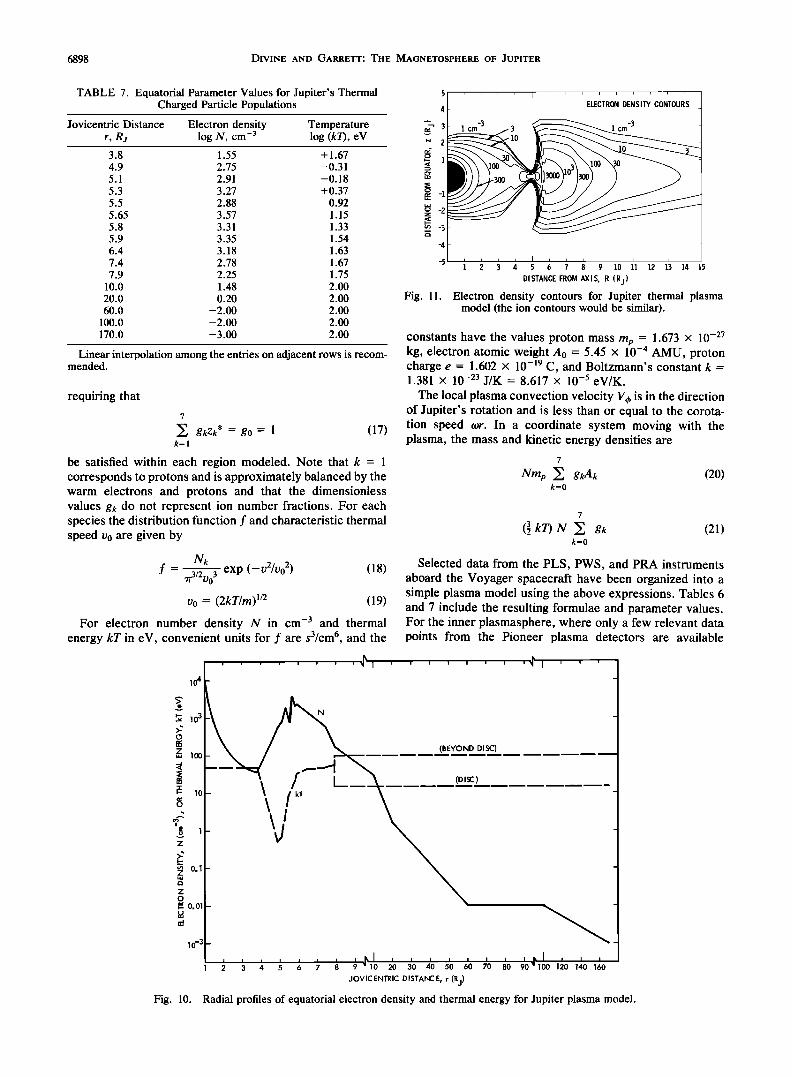
DISTANCE FROM AXIS, R {Rj) Fig. 11. Electron density contours for Jupiter thermal plasma

model (the ion contours would be similar).

constants have the values proton mass m e = 1.673 x 10 -27 kg, electron atomic weight A0 = 5.45 x 10 -4 AMU, proton charge e = 1.602 x 10 -•9 C, and Boltzmann's constant k - 1.381 x 10 -23 J/K = 8.617 x 10 -5 eV/K.

The local plasma convection velocity V, is in the direction of Jupiter's rotation and is less than or equal to the corotation speed •or. In a coordinate system moving with the plasma, the mass and kinetic energy densities are

7

Nmv • gkAk (20) k=0

7

(3 kT) N • gk 2 k=0

(21)

Selected data from the PLS, PWS, and PRA instruments aboard the Voyager spacecraft have been organized into a simple plasma model using ,the above expressions. Tables 6 and 7 include the resulting formulae and parameter values. For the inner plasmasphere, where only a few relevant data points from the Pioneer plasma detectors are available

•. 03 N -• 1

Z

'" 1 •- 10 O

Z

,n 0ol- Z

Z

I-. 0.01 -

10-3 -

(BEYOND DISC)

(DISC)

, , , , , , , I , • , , 2 3 4 5 6 7 $ } •10 20 3•0 20 5•0 20 )0 •0 •0•1 0 120 110 160 JOVICENTRIC DISTANCE, r (R j)

Fig. 10. Radial profiles of equatorial electron density and thermal energy for Jupiter plasma model.


15

108 E >1.5 MeV •..M,• N -

ß

ø -15 -10 -5 0 5 10 15

TIME FROM PERI JOVE {hours)

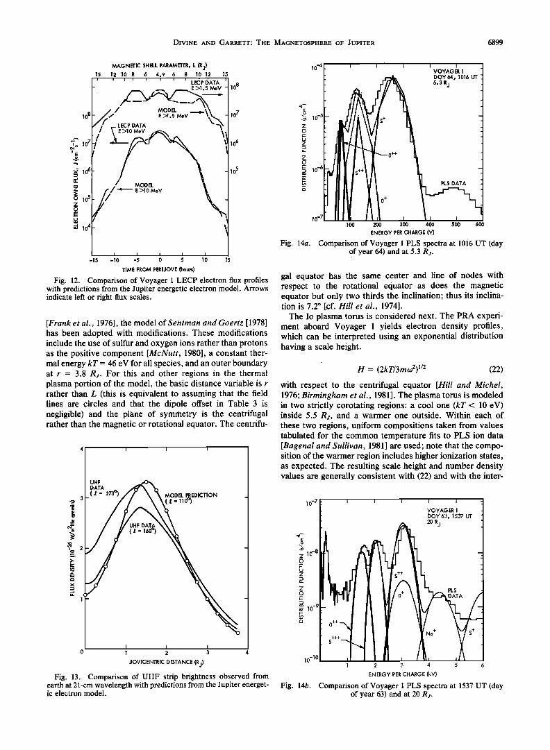
Fig. 12. Comparison of Voyager 1 LECP electron flux profiles with predictions from the Jupiter energetic electron model. Arrows indicate left or right flux scales.

MAGNETIC SHELL PARAMETER, L (R j) 10-4 I I I I I VOYAGER I 12 10 8 6 4ø9 6 8 10 12 15 DOY64 t 1016 UT ' ' ' ' ' ' • LEaP I•ATA' ' 08 5ø3 Rj E>I.5MeV - 1

107 -• • 10 -5 - .

106 Z• • ø•

105 • 10 '6

lO -7 ! ! • 100 200 300 400 500 600

ENERGY PER CHARGE (V)

Fig. 14a. ',or of %oy: ger I t'L,S spe of year 64) and at 5.3 Rj.

[Frank et al., 1976], the model of Sentman and Goertz [1978] has been adopted with modifications. These modifications include the use of sulfur and oxygen ions rather than protons as the positive component [McNutt, 1980], a constant thermal energy kT = 46 eV for all species, and an outer boundary at r = 3.8 Rj. For this and other regions in the thermal plasma portion of the model, the basic distance variable is r rather than L (this is equivalent to assuming that the field lines are circles and that the dipole offset in Table 3 is negligible) and the plane of symmetry is the centrifugal rather than the magnetic or rotational equator. The centrifu-

Comparison of Voyager 1 PLS spectra at 1016 UT (day

gal equator has the same center and line of nodes with respect to the rotational equator as does the magnetic equator. but only two thirds the inclination; thus its inclination is 7.2 ø [cf. Hill et al., 1974].

The Io plasma torus is considered next. The PRA experiment aboard Voyager 1 yields electron density profiles, which can be interpreted using an exponential distribution having a scale height.

H = (2kT/3moo2) 1/2 (22) with respect to the centrifugal equator [Hill and Michel, 1976; Birmingham et al., 1981]. The plasma torus is modeled in two strictly corotating regions: a cool one (kT < 10 eV) inside 5.5 Rj, and a warmer one outside. Within each of these two regions, uniform compositions taken from values tabulated for the common temperature fits to PLS ion data

• , , , ] [BagenalandSullivan, 1981]areused;notethattheCompo- sition of the warmer region includes higher ionization states, as expected. The resulting scale height and number density values are generally consistent with (22) and with the inter-

l UHF • I

i DATA ß . l ( '• = 2730) /•'" X • MODEL ,REDICTION • = 10-7 ] ] [ ] I • VOYAGER I DOY 63• 1537 UT

• 20 Rj

• • • RES

JOVIcENTRIC DISTANCE (R j) 1• '101 I • • • t _ 2 3 4 5 6

Fig. 13. Comparison of UHF strip brightness observed from ENERGY PER CHARGE •V) each at 21-cm wavelength with predictions from the Jupiter energet- Fig. 14b. Comparison of Voyager 1 PLS spectra at 1537 UT (day ic electron model. of year 63) and at 20 R•.


GALILEO RADIATION SPECTRA

10 I-5 10 I-5

•'E 1014 Z 0

u

,,, 1013

0

Z 1012

JOI + 5 ORBITS

io 14

!013

1012

•o • I I I I I I •o• i 2 3 4 5 6

ENERGY (MeV)

Fig. 15. Integral electron fluences at various times in the Galileo mission (JOI = Jupiter orbit insertion). Thirteen orbits corresponds to roughly a 2-year mission.

pretation of Sullivan and Siscoe [1982] and are illustrated in Figure 10.

The inner disc represents a transition region outside the warm torus in which corotation weakens moving outward, consistent with PLS results, and the temperature in the disc is much smaller than outside it [Scudder eta!., 1981]. Its composition has been matched to that from the PLS ion data at 19.8 Rs [Bagenal and Sullivan, 1981], and the symmetry surface makes the transition from the centrifugal equator to the wavy disc, as suggested in the last of the four models presented by Carbary [1980]. That geometry has been used for the outer disc as well, and there the constant value 200 km/s for the azimuthal convection speed is used [McNutt et al., 1981]. In this region, a crude fit to the electron density results from the Voyager PLS and PWS data has been used, ignoring any dependence on local time. Because the location of the magnetopause varies strongly with both local time and the dynamic pressure of the solar wind, its size and shape, and that of the magnetotail, have not been modeled here.

Figure 10 illustrates the radial dependence of the electron number density and thermal energy kT for these models. Figure 11 presents contours of constant number density in a plane perpendicular to the symmetry surface.

COMPARISONS WITH DATA

In this section, a few of the many possible comparisons of the model with Jovian data are presented. These comparisons will be limited to the radiation belt and thermal portions of the model, as there is too little data to compare adequately with the warm plasma portion. For the radiation belt models, Figure 12 shows the predicted profile of integral electron flux during the Voyager 1 flyby of Jupiter (for energy thresholds corresponding to two channels of the Voyager LECP) and the fluxes derived by the LECP investigators from their data [Krimigis et al., 1979b]. The quantitative differences between the model and observed profiles are within a factor of 2 and are representative of the uncertainty of the Pioneer and

Voyager data sets and of the models themselves. The differences in the shapes of the peaks in these profiles suggest the magnitude of likely longitudinal or temporal variations or of defects in the model or its data set. Figure 13 shows the predicted profile of synchrotron emission from the energetic electron model for a wavelength of 21 cm and as would be observed from earth at a distance of 4.04 AU and l = 110 ̧ for a half-power beam width of 1.2 Rs, compared with observed data for two longitudes [dePater and Dames, 1979]. The predicted results reflect the fact that the model parameters, which control the electron pitch angle and latitude distributions inside the Pioneer 10 perijove (for L < 2.85 they are not strongly constrained by the Pioneer 11 data), have been adjusted to represent better the data. Even so, the fact that the discrepancies are still about a factor of 2 demonstrates that the match to the profiles and to the spectrum and polarization of the earth-based UHF data is imperfect.

In Figure 14 the predictions of the low-energy ion model are compared with actual data [McNutt et al., 1981; Bagenal and Sullivan, 1981]. For the model these examples correspond to the cool torus (5.3 Rs) and inner disc (20 Rs). The Voyager data are well fit, although at 5.3 Rs the model slightly overestimates and at 20 Rj underestimates the observed convection velocity into the detectors (this may be a result of ignoring the details of the spacecraft/plasma relative velocity vector; only corotation and the vehicle angular velocities were included). Even so, the model adequately reproduces the various plasma features for two very different plasma regimes to an accuracy of a factor of 2 or better (note that the cold proton component has not been included in these examples). Considering the simplicity of the model', this is quite good agreement. Similar results were obtained for other representative spectra.

COMPARISON OF ELECTRON DOSE VS AL SHIELD THICKNESS

i08

i07

• 106 -• MINIMUM PARTS CAPABILITY

150 kRAD (SJ)

) 10 5 IONIZATION DOSE

J- •/'•, -J 'DESIGN POINT

L EMS STRAH LUNG

103 10 -2 10 -I 100 10 I

ALUMINUM SPHERICAL SHELL THICKNESS (g/cm 2)

Fig. 16. Jovian electron dose versus aluminum shield thickness for the Galileo mission, as predicted by the model.

_


JOVIAN MODEL APPLICATIONS

The Jovian model presented in this paper was developed specifically for several practical applications. These applications range from the common need for radiation design guidelines to the more esoteric areas of single event upsets and spacecraft charging. An example of the predictions of the model for these phenomena will be presented. As the purpose of this paper is not to study these interactions but rather to demonstrate the utility of the model, no attempt will be made to justify the calculations involved. Rather the reader is referred to relevant literature in each area.

The first and most common application of the model is in the calculation of the effects of energetic particle radiation. As the major effect is normally the result of electron ionization, the example is limited to electrons. In Figure 15 the model results have been translated into total integral fluence (electron/cm 2) as a function of energy and time for the Galileo mission profile. In Figure 16 these results have been used to calculate the total dose experienced by Galileo electronic components for different levels of shielding after closest encounter plus 5 orbits and after 2 years (closest encounter plus 13 orbits). A typical shielding level for Galileo is 3 g/cm 2. For the hardness levels of the Galileo electronic components, this implies (Figure 16) a mission life of at least 2 years. The use and impact of the.model on the radiation hardness design of Galileo is obvious.

A recent problem of considerable concern for spacecraft in the Jovian environment has been surface charging. Sur- face potentials of the order of 20 kV have been observed at the earth [Reasoner et al., 1976] and were anticipated in the Jovian environment. Spacecraft charging models and theoretical considerations are detailed by Garrett [1981]. A simple spacecraft to space thick sheath model (including the secondary emission properties of aluminum) described in that paper was used to estimate potentials in the Jovian environment. As over a large portion of the Jovian magnetosphere the warm to energetic electron fluxes are the domi- nate current source, balancing principally with the photo-

JOVIAN SATELLITE/SPACE POTENTIALS FOR THICK SHEATH

(PHOTOELECTRONS AND SECONDARIES INCLUDED)

6 4 10

2

-2 _•,,,,Clg - •--,Q_• _10 -4 -10 • • • -6 _-10

-10 I I I I I I I 0 2 4 6 8 10 12 14 16

Fig. 17. Spacecraft to space potential contours for the thick sheath approximation in the ! = 110øW meridian. The horizontal axis represents distance along the rotational equator. Photoelectron and secondary electron currents are included. The dashed lines bracket the region of applicability (no observations were available outside this latitude region). Positive potential values greater than 10 V are not accurately predicted by the simple charging model.

JOVIAN SATELLITE/SPACE POTENTIALS FOR THICK SHEATH

(NO PHOTOELECTRONS AND NO SECONDARIES)

Rj 0 -4•7'• 3 -103

? 0 2 4 6 8 10 12 14 16

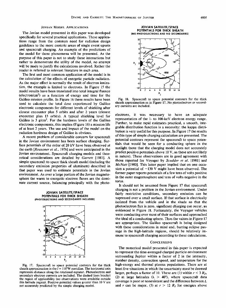
Rj Fig. 18. Spac•ecraft to space potential contours for the thick

sheath approximation as in Figure 17. No photoelectron or secondary currents are included.

electrons, it was necessary to have an adequate representation of the 1- to 100-keV electron energy range. Further, to make rapid estimates practical, a smooth, inte- grable distribution function is a necessity: the kappa distribution is very useful for this purpose. In Figure 17 the results of this type of simple charging calculation are presented. The potential contours represent the spacecraft to space potentials that would be seen for a conducting sphere in the sunlight (note that the charging model does not accurately predict positive potentials above 10 V, as these are not likely in nature). These observations are in good agreement with those reported for Voyager by Scudder et al. [1981] and McNutt [1980]. This latter paper implied that on one occa- sion a potential of -130 V might have been observed. The former paper reports potentials of a few tens of volts positive in the outer magnetosphere and tens of volts negative in the torus.

It should not be assumed from Figure 17 that spacecraft charging is not a problem in the Jovian environment. Under fairly restrictive conditions, secondary emission can be supressed over a small surface. If that surface is electrically isolated from the vehicle and in the shade so that the photoelectron flux is zero, significant ch•trging can occur, as evidenced in Figure 18. Fortunately, the Voyager vehicles were conducting over most of their surfaces and approached the ideal of a conducting sphere. Thus the values in Figure 17 are appropriate. The Galileo spacecraft is being designed with these considerations in mind and, barring eclipse passage in the high-latitude regions, should be relatively im- mune to spacecraft charging according to these calculations.

CONCLUSIONS

The numerical model presented in this paper is expected to represent the time-averaged charged particle environment surrounding Jupiter within a factor of 2 in the intensity, number density, convection speed, and temperature for the high-energy and thermal plasma populations. There are at least five situations in which the uncertainty must be deemed larger, perhaps a factor of 10. These are (1) within r < 3 R j, (2) at large latitudes (h • 40ø), where spacecraft data coverage is poor or nonexistent and the difference between L and r can be major, (3) at r • 12 Rj for energies above


several keV where temporal variations in count rates are so large as to make static models such as these irrelevant, (4) at r > 50 Rj for all energies, where local time and solar wind variations can be significant, and (5), reflecting the paucity of data, for the warm plasma population. In addition, it is suggested that although the magnetic field and radiation belt models may be considered fairly mature, the thermal and warm plasma models will require further development as more analyzed data are published.

Despite the shortcomings just listed, it has been demon- strated that the model does make valuable contributions to our overall understanding of the Jovian environment. In particular, the model has already made significant contributions to the design of future Jovian missions. It has resulted in design modifications that should make such missions much more survivable in the hostile Jovian environment. The model represents an important reference standard for future studies of Jupiter as it makes available in a compact form much of the published data on the Jovian environment (the authors will make available on request FORTRAN listings of the various components of the model). Finally, the nature of the model makes it readily modifiable when more detailed data become available.

Acknowledgments. We wish to thank M. H. Acuna, H. S. Bridge, R. W. Fillius, S. M. Krimigis, F. B. McDonald, J. A. Simpson, E. J. Smith, E. C. Stone, J. D. Sullivan, J. A. Van Allen, D. J. Williams, and the associated experiment teams for contributing their insight and spacecraft data (often in advance of, or in more detail than, the relevant publications) in the development of these models; E. J. Franzgrote for analytic simulations of electron response functions of various Pioneer detectors; E. T. Olsen for calculation of synchrotron radiation intensities from the inner energetic electron distributions; C. O. Stearns and M. C. Deutsch for programing fits to the plasma data and models; and J. F. Carbary and E. C. Stone for their constructive comments on an earlier version of this work. This report represents the results of one phase of research carried out at the Jet Propulsion Laboratory, California Institute of Technology under NASA contract NAS 7-100.

The Editor thanks D. Hamilton and J. F. Carbary for their assistance in evaluating this paper.

REFERENCES

Acuna, M. H., and N. F. Ness, The main magnetic field of Jupiter, J. Geophys. Res., 81, 2917-2922, 1976a.

Acuna, M. H., and N. F. Ness, Results from the GSFC fluxgate magnetometer on Pioneer 11, in Jupiter, edited by T. Gehrels, pp. 830-847, University of Arizona Press, Tucson, 1976b.

Bagenal, F., and J. D. Sullivan, Direct plasma measurements in the Io torus and inner magnetosphere of Jupiter, J. Geophys. Res., 86, 8447-8466, 1981.

Baker, D. N., and J. A. Van Allen, Revised Pioneer 10 absolute electron intensities in the inner Jovian magnetosphere, J. Geophys. Res., 82, 681-683, 1977.

Beck, A. J. (Ed.), Proceedings of the Jupiter radiation belt work- shop, Tech. Memo. 33-543, Jet Propulsion Lab., NASA, Pasade- na, Calif., 1972.

Behannon, K. W., L. F. Burlaga, and N. F. Ness, The Jovian magnetotail and its current sheet, J. Geophys. Res., 86, 8385- 8401, 1981.

Berge, G. L., and S. Gulkis, Earth-based radio observations of jupiter: Millimeter to meter wavelengths, in Jupiter, edited by T. Gehrels, pp. 621-692, University of Arizona Press, Tucson, 1976.

Birmingham, T. J., J. K. Alexander, M.D. Desch, R. F. Hubbard, and B. M. Pedersen, Observations of electron gyroharmonic waves and the structure of the Io torus, J. Geophys. Res., 86, 8497-8507, 1981.

Brice, N.M., and G. A. Ioannidis, The magnetospheres of Jupiter and earth, Icarus, 13, 173-183, 1970.

Bridge, H. S., J. W. Belcher, A. J. Lazarus, J. D. Sullivan, R. L. McNutt, F. Bagenal, J. D. Scudder, E. C. Sittler, G. L. Siscoe, V.

M. Vasylivnas, C. K. Goertz, and C. M. Yeats, Plasma observations near Jupiter: Initial results from Voyager 1, Science, 204, 987-991, 1979a.

Bridge, H. S., J. W. Belcher, A. J. Lazarus, J, D. Sullivan, F. Bagenal, R. L. McNutt, Jr., K. W. Ogilvie, J. D. Scudder, E. C. Sittier, V. M. Vasyiiunas, and C. K. Goertz, Plasma observations near Jupiter: Initial results from Voyager 2, Science, 206, 972- 976, 1979b.

Carbary, J. F., Periodicities in the Jovian magnetosphere: Magneto- disc models after Voyager, Geophys. Res. Lett., 7, 29-32, 1980.

Carbary, J. F., T. W. Hill, and A. J. Dessler, Planetary spin period acceleration of particles in the Jovian magnetosphere, J. Geophys. Res., 81, 5189-5195, 1976.

Connerney, J. E. P., M. H. Acuna, and N. F. Ness, Modeling the Jovian current sheet and inner magnetosphere, J. Geophys. Res., 86, 8370-8384, 1981.

Coroniti, F. V., Energetic electrons in Jupiter's magnetosphere, Astrophys. J. Suppl., 27, 261-281, 1974.

dePater, I., and H. A. C. Dames, Jupiter's radiation belts and atmosphere, Astron. Astrophys., 72, 148-160, 1979.

Dessler, A. J., and V. M. Vasyliunas, The magnetic anomaly model of the Jovian magnetosphere: Predictions for Voyager, Geophys. Res. Lett., 6, 37-40, 1979.

Drake, F. D., and H. Hvatum, Non-thermal microwave radiation from Jupiter, Astron. J., 64, 329-330, 1959.

Fillius, R. W., The trapped radiation belts of Jupiter, in Jupiter, edited by T. Gehrels, pp. 896-927, University of Arizona Press, Tucson, 1976.

Fillius, R. W., and C. E. Mcllwain, Measurements of the Jovian radiation belts, J. Geophys. Res., 79, 3589-3599, 1974.

Fillius, R. W., C. E. Mcllwain, and A. Mogro-Campero, Radiation belts of Jupiter: A second look, Science, 188, 465-467, 1975.

Formisano, V. (Ed.), The Magnetospheres of the Earth and Jupiter, D. Reidel, Hingham, Mass., 1975.

Frank, L. A., K. L. Ackerson, J. H. Wolfe, and J. D. Mihalov, Observations of plasmas in the Jovian magnetosphere, J. Geophys. Res., 81,457-468, 1976.

Garrett, H. B., The charging of spacecraft surfaces, Rev. Geophys. Space Phys., 19, 577-616, 1981.

Gehrels, N., E. C. Stone, and J. H. Trainor, Energetic oxygen and sulfur in the Jovian magnetosphere, J. Geophys. Res., 86, 8906- 8918, 1981.

Gehrels, T. (Ed.), Jupiter, University of Arizona Press, Tucson, 1976.

Goertz, C. K., and M. F. Thomsen, The dynamics of the Jovian magnetosphere, Rev. Geophys. Space Phys., 17, 731-743, 1979.

Gurnett, D. A., W. S. Kurth, and F. L. Scarf, Plasma wave observations near Jupiter: Initial results from Voyager 2, Science, 206, 987-991, 1979.

Hill, T. W., Interchange stability of a rapidly rotating magnetosphere, Planet. Space Sci., 24, 1151-1154, 1976.

Hill, T. W., Intertial limit on corotation, J. Geophys. Res., 84, 6554- 6558, 1979.

Hill, T. W., and J. F. Carbary, Centrifugal distortion of the Jovian magnetosphere by an equatorially confined current sheet, J. Geophys. Res., 83, 5745-5749, 1978.

Hill, T. W., and F. C. Michel, Heavy ions from the Galilean satellites and the centrifugal distortion of the Jovian magnetosphere, J. Geophys. Res., 81, 4561-4565, 1976.

Hill, T. W., A. J. Dessler, and F. C. Michel, Configuration of the Jovian magnetosphere, Geophys. Re•. Lett., 1, 3-6, 1974.

Ioannidis, G., and N. Brice, Plasma densities in the Jovian magnetosphere: Plasma slingshot or Maxwell demon?, Icarus, 14, 360- 363, 1971.

Kennel, C. F., and F. V. Coroniti, Is Jupiter's magnetosphere like a pulsar's or earth's, Space Sci. Rev., 17, 857-883, 1975.

Krimigis, S. M., T. P. Armstrong, W. I. Axford, C. O. Bostrom, C. Y. Fan, G. Gloeckler, L. J. Lanzerotti, E. P. Keath, R. D. Zwickl, J. F. Carbary, and D.C. Hamilton, Low-energy charged particle environment at Jupiter: A first look, Science, 204, 998- 1003, 1979a.

Krimigis, S. M., T. P. Armstrong, W. I. Axford, C. O. Bostrom, C. Y. Fan, G. Gloeckler, L. J. Lanzerotti, E. P. Keath, R. D. Zwickl, J. F. Carbary, and D.C. Hamilton, Hot plasma environment at Jupiter: Voyager 2 results, Science, 206, 977-984, 1979b.

Krimigis, S. M., J. F. Carbary, E. P. Keath, C. O. Bostrom, W. I. Axford, G. Gloeckler, L. J. Lanzerotti, and T. P. Armstrong,


Characteristics of hot plasma in the Jovian magnetosphere: Re- sults from the Voyager spacecraft, J. Geophys. Res., 86, 8227- 8257, 1981.

McDonald, F. B., and J. H. Trainor, Observations of energetic Jovian electrons and protons, in Jupiter, edited by T. Gehrels, pp. 961-987, University of Arizona Press, Tucson, 1976.

McNutt, R. L., Jr., The dynamics of the low energy plasma in the Jovian magnetosphere, Ph.D. thesis, Mass. Inst. of Technol., Cambridge, 1980.

McNutt, R. L., Jr., J. W. Belcher, and H. S. Bridge, Positve ion observations in the middle magnetosphere of Jupiter, J. Geophys. Res., 86, 8319-8342, 1981.

Ness, N. F., M. H. Acuna, R. P. Lepping, L. F. Burlaga, K. W. Behannon, and F. M. Neubauer, Magnetic field studies at Jupiter by Voyager 1: Preliminary results, Science, 204, 982-987, 1979a.

Ness, N. F., M. H. Acuna, R. P. Lepping, L. F. Burlaga, K. W. Behannon, and F. M. Neubauer, Magnetic field studies at Jupiter by Voyager 2: Preliminary results, Science, 206, 966-972, 1979b.

Neugebauer, M., and A. Eviatar, An alternative interpretation of Jupiter's 'plasmapause,' Geophys. Res. Lett., 3, 708-710, 1976.

Pyle, K. R., R. B. McKibben, and J. A. Simpson, Pioneer 11 observations of trapped particle absorption by the Jovian ring and the satellites 1979, J1, J2, and J3, J. Geophys. Res., 88, 45-48, 1983.

Reasoner, D. L., W. Lennartsson, and C. R. Chappell, Relationship between ATS-6 spacecraft-charging occurrences and warm plasma encounters, in Spacecraft Charging by Magnetospheric Plas- mas, Prog. Astronaut. Aeronaut, vol. 47, edited by A. Rosen, pp. 89-101, MIT Press, Cambridge, Mass., 1976.

Richardson, J. D., and G. L. Siscoe, Factors governing the ratio of inward to outward diffusing flux of satellite ions, J. Geophys. Res., 86, 8485-8490, 1981.

Scarf, F. L., D. A. Gurnett, and W. S. Kurth, Jupiter plasma wave observations: An initial Voyager 1 overview, Science, 204, 991- 995, 1979.

Scudder, J. D., E. C. Sittier, Jr., and H. S. Bridge, A survey of the plasma electron environment of Jupiter: A view from Voyager, J. Geophys. Res., 86, 8157-8179, 1981.

Seidelmann, P. K., and N. Divine, Evaluation of Jupiter longitudes in System III (1965), Geophys. Res. Lett., 4, 65-68, 1977.

Sentman, D. D., and C. K. Goertz, Whistler mode noise in Jupiter's inner magnetosphere, J. Geophys. Res., 83, 3151-3165, 1978.

Simpson, J. A., and R. B. McKibben, Dynamics of the Jovian magnetosphere and energetic particle radiation, in Jupiter, edited by T. Gehrels, pp. 738-766, University of Arizona Press, Tucson, 1976.

Simpson, J. A., D.C. Hamilton, R. B. McKibben, A. Mogro- Campero, K. R. Pyle, and A. J. Tuzzolino, The protons and electrons trapped in the Jovian dipole magnetic field region and their interaction with Io, J. Geophys. Res., 79, 3522-3544, 1974.

Simpson, J. A., D.C. Hamilton, G. A. Lentz, R. B. McKibben, M. Perkins, K. R. Pyle, A. J. Tuzzolino, and J. J. O'Gallagher, Jupiter revisited: First results from the University of Chicago charged particle experiment on Pioneer 11, Science, 188, 455-459, 1975.

Siscoe, G. L., and D. Summers, Centrifugally driven diffusion of iogenic plasma, J. Geophys. Res., 86, 8471-8479, 1981.

Smith, E. J., L. Davis, Jr., and D. E. Jones, Jupiter's magnetic field

and magnetosphere, in Jupiter, edited by T. Gehrels, pp. 788-829, University of Arizona Press, Tucson, 1976.

Sullivan, J. D., and G. L. Siscoe, In situ observations of Io torus plasma, in The Satellites of Jupiter, edited by D. Morrison, pp. 846-871, University of Arizona Press, Tucson, 1982.

Thomsen, M. F., and C. K. Goertz, Further observational support for the limited-latitude magnetodisc model of the outer Jovian magnetosphere, J. Geophys. Res., 86, 7519-7526, 1981.

Trainor, J. H., F. B. McDonald, B. J. Teegarden, W. R. Webber, and E. C. Roelof, Energetic particles in the Jovian magnetosphere, J. Geophys. Res., 79, 3600-3613, 1974.

Trainor, J. H., F. B. McDonald, D. E. Stilwell, B. J. Teegarden, and W. R. Webber, Jovian protons and electrons: Pioneer 11, Science, 188, 462-465, 1975.

Van Allen, J. A., High-energy particles in the Jovian magnetosphere, in Jupiter, edited by T. Gehrels, pp. 928-960, University of Arizona Press, Tucson, 1976.

Van Allen, J. A., D. N. Baker, B. A. Randall, M. F. Thomsen, and D. D. Sentman, The magnetosphere of Jupiter as observed with Pioneer 10, 1, Instrument and principal findings, J. Geophys. Res., 79, 3559-3577, 1974.

Van Allen, J. A., B. A. Randall, D. N. Baker, C. K. Goertz, D. D. Sentman, M. F. Thomsen, and H. R. Flindt, Pioneer 11 observations of energetic particles in the Jovian magnetosphere, Science, 188, 459-462, 1975.

Vasyliunas, V. M., A survey of low-energy electrons in the evening sector of the magnetosphere with OGO 1 and OGO 3, J. Geophys. Res., 73, 2839-2884, 1968.

Vasyliunas, V. M., and A. J. Dessler, The magnetic anomaly model of the Jovian magnetosphere: A post-Voyager assessment, J. Geophys. Res., 86, 8435-8446, 1981.

Vogt, R. E., W. R. Cook, A. C. Cummings, T. L. Garrard, N. Gehrels, E. C. Stone, J. H. Trainor, A. W. Schardt, T. F. ConIon, N. Lal, and F. B. McDonald, Voyager 1: Energetic ions and electrons in the Jovian magnetosphere, Science, 204, 1003-1007, 1979a.

Vogt, R. E., A. C. Cummings, T. L. Garrard, N. Gehrels, E. C. Stone, J. H. Trainor, A. W. Schardt, T. F. Conlon, and F. B. McDonald, Voyager 2: Energetic ions and electrons in the Jovian magnetosphere, Science, 206, 984-987, 1979b.

Warwick, J. W., J. B. Pearce, A. C. Riddle, J. K. Alexander, M.D. Desch, M. L. Kaiser, J. R. Theiman, T. D. Carr, S. Gulkis, A. Boischot, C. C. Harvey, and B. M. Pedersen, Voyager 1 planetary radio astronomy observations near Jupiter, Science, 204, 995-998, 1979a.

Warwick, J. W., J. B. Pearce, A. C. Riddle, J. K. Alexander, M.D. Desch, M. L. Kaiser, J. R. Theiman, T. D. Carr, S. Gulkis, A. Boischot, Y. Leblanc, B. M. Pedersen, and D. H. Staelin, Planetary radio astronomy observations from Voyager 2 near Jupiter, Science, 206, 991-995, 1979b.

N. Divine and H. B. Garrett, Jet Propulsion Laboratory (144-218), California Institute of Technology, 4800 Oak Grove Dr., Pasadena, CA 91109.

(Received January 7, 1983; revised May 23, 1983;

accepted June 1, 1983.)

journal of geophysical research, vol. 88, no. …lyutikov/liter/jupiterbelt.pdf · journal of...

Documents