JOURNAL OF GEOPHYSICAL RESEARCH, VOL. 88, NO. B12, PAGES 10,323-10,332, DECEMBER 10, 1983

Minimal Upper Mantle Temperature Variations Consistent With Observed Heat Flow and Plate Velocities

WILLIAM M. KAULA

Department of Earth & Space Sciences, University of California, Los Angeles

The momentum equations applied to 5 ø block means are integrated from the observed surface plate velocities downward to a depth of 280 km, assuming no lateral heterogeneities in density or viscosity. It is assumed that 85% of the global heat production Qc, = 0.85 x 4.0 x 10 •3 W comes from below 280 km and that at this level the transfer is fully convective. A temperature field T is inferred at depth 280 km by minimizing the quantity fit - Tol" dS + nX{Qc, - pCf(T - To)v,.dS}, where the integrals are over the sphere, p is density, C is heat capacity, v, is radial velocity, To is a prescribed mean, and X is a Lagrangian multiplier. Norms n, ranging from 1.5 to 2.5, are tried. The intervening temperature fields are then inferred, integrating the energy equation downward by using the previously calculated velocity field. This integration is subject to the limitations that the derivative of the temperature with respect to depth is everywhere sufficient to attain the fully convecting temperature, but never less than adiabatic. A surface heat flow based on observations plus age and tectonic setting is used. The principal inferences are: (1) the greatest lateral variations in temperature, -1000øC, occur with the top 20 km; (2) the greatest advection, -200øC/m.y., occurs within the top 20 km; (3) below 50 km, the greatest departures of temperature from the mean are negative "tongues," reaching an extreme of about -800øC at depth 100 km; (4) below 50 km, heat transfer becomes more convective than conductive; (5) at the fully convecting level, 280 km, temperature variations are at least _+ 180øC about the mean. The principal defect in the entire calculation is unrealistically low temperatures arising from unrepresentatively low surface heat flows. The principal defect of the model probably arises from the assumption that all heat transfer at a depth of 280 km is representable by 5 ø means in velocity and temperature.

INTRODUCTION

The purpose of this paper is to infer upper mantle tempera- ture variations from plate velocities and heat flow data. My intent is to use these temperature distributions as a starting model for interpreting variations of the gravity field. They should also be of interest for interpreting petrological, seis- mological, and other data.

The guiding principles of the approximate calculation carried out in this paper is that it be as complete as possible, subject to three main limitations: (1) the equations of motion are decoupled from the energy equation; (2) the boundary layer variation in temperature with depth is determined by local conditions; and (3) the resolution is limited to that expressible by 5 ø square means (or 36th degree harmonics). Even with these limitations, the work is a considerable elaboration on any similar analyses previously made. A two- stage calculation results.

In the first stage, velocities as functions of radius, latitude, and longitude (or alternatively, radius, harmonic degree, and order) are calculated by starting from zero vertical velocity and given horizontal velocities at the surface and using the mass and momentum conservation equations with densities and viscosities prescribed as functions of depth only. In the second stage the temperatures are calculated by starting from uniform temperature and given heat flow at the surface and using the energy equation with the already calculated velocities and prescribed heat sources and thermal proper- ties (densities, heat capacities, and conductivities) at depth. The first-stage calculation is essentially identical to that of Hager and O'Connell [1978, 1979]. The second-stage calcu-

Copyright 1983 by the American Geophysical Union.

Paper number 3B 1054. 0148-0227/83/003 B- 1054505.00

lation has some similarities to those of Chapman and Pollack [1975, 1980], Pollack and Chapman [1977], and Sclater et al. [1980]. It differs, however, in taking more explicit account of the velocity field.

The second stage, as stated above, is insufficient, howev- er, to obtain a temperature distribution approximating that of a convecting regime. A global condition characteristic of this regime must be applied. The principal idea applied in this work is that of a fully convecting level. For such a level r,. we can write, for the total global heat flow QG:

pCv,.Trc 2 dS • Qa 2 - Rr 2 dr dS = QG (1)

where p is density, C is heat capacity, v,. is radial velocity, T is temperature, Q is surface heat flow, R is the density of intrinsic heat sources, a is surface radius, and the integrals are over the unit sr•here. In this studv. 280 km was chosen as

the fully convecting level, as a reasonable compromise. At this depth the only regions of perceptible conductive transfer would be under old continents, which are of slight effect on the global heat budget. To go deeper, however, would risk more error in the velocity field extrapolated from the surface plate motions.

There are three principal objections to the program out- lined here: (1) the heat flow is affected by relatively shallow phenomena; (2) the velocity field is affected by lateral variations in lithospheric theology; and (3) the temperature variation with respect to depth is affected by location with respect to the velocity field.

Oceanic heat flow measurements can be unrepresentative- ly low because of convection in the shallow permeable layer. An adjustment for these effects near ocean rises is made in the heat flow compilation of Chapman and Pollack [1980], which is the one used. The question is to what extent is adjustment needed well off the rise, perhaps as far as 80

10,323

10,324 KAULA' MINIMAL UPPER MANTLE TEMPERATURE VARIATIONS

million years [Anderson and Skilbeck, 1981; Embley et al., 1983]. The answer depends on detailed examination of the circumstances of the observations. Meanwhile, it is an open question as to whether some of the low heat flow values to

the flanks of ocean rises indicate secondary return flows. On the continents there are marked heat flow variations arising from crustal sources [Sclater et al. 1981] as well as mantle- lithosphere interaction. In view thereof I assume a uniform heat flow at the base of the continental crust. Despite the appreciable irregularities of shallow origin, the heat flow must still be a strong constraint on upper mantle tempera- tures.

Lateral variations in lithospheric rheology, arising mainly from temperature dependence, result in marked lateral varia- tions in stress [Hager and O'Connell, 1981] and hence must affect the velocity field. However, in the present calculation the stress field is not of interest per se, while its effects on the velocity field are not manifest until they are integrated over some distance. For this reason, the integrations of Hager and O'Connell [1978, 1979], with only radial variation in viscosity, were successful in reproducing the flow pattern in subduction zones. In the present calculation the main effect of lithospheric rheology is taken into account by starting from the surface velocity field in which nonzero divergence is confined to plate margins. Hence the error is in the second-order variations.

In integrating the energy equation downward by using the 5 ø averaged velocity field, provision must be made for contributions to the averaged advection v ß VT from smaller- scale variations. This provision necessitates assumptions that are based on boundary layer theory [e.g., Olson and Cotcos, 1980], computer experiment [e.g., McKenzie et al., 1974], or more local analyses of data [e.g., Lewis, 1981]. The theoretical and computer models indicate that temperature variation with respect to depth does not increase monotoni- cally to the flanks of a plume, but the detailed data analyses, nonetheless, get a good fit with a monotonic increase. A global-scale model cannot hope to do better; in any case the variation of temperature from a monotonic gradient is small compared to the total temperature change between surface and asthenosphere.

FUNDAMENTAL EQUATIONS

Under the assumptions stated in the introduction, the conservation equations (7)-(9) in Kaula [1980] reduce to

0 = v ß (pv) (2)

0 = -V•Sp + O{rlOv,./Or}/Or + r/V•t2v (3)

pCOT/Ot = •' (K•T) + qR + Z (4)

where v is velocity, Sp is the variation of pressure from hydrostatic, r/is viscosity, K is thermal conductivity, qR is the radioactive heat source, and Z is the nonlinear term'

z = -oCr. {VT- ,•r,,'} + ,VIE' El/2 (5)

where I is the radial unit vector, T,' is the adiabatic gradient, and V: is the strain rate tensor.

MOMENTUM INTEGRATION

The integration of the poloidal velocity field was first done in terms of spherical harmonics, which results in sets of four first-order differential equations: one set for each harmonic

degree and order, as described in Kaula [1975a] and Hager and O'Connell [1978, 1979]. The viscosities used were as given in Kaula [1980].

However, this procedure resulted in some unrealistic oscillations in vr ("Gibbs effects") to the flanks of rapidly spreading rises. These oscillations persisted to some extent, even when the surface harmonic coefficients were obtained

by harmonic analysis of divergence along plate margins using 1 ø intervals:

v• t 1 f = w Y• dB (6) 4rrL

where the notation is as in Kaula [1975a, 1980]: v, • is the poloidal velocity scalar; I in the indices is an abbreviation for degree and order l, m; L is l(l + 1); w is the spreading velocity, positive on a rise; Y• is the spherical harmonic; and the integration is along all plate margins. Equation (6) is obtained by applying the divergence theorem to the usual equation in terms of derivatives [(12) in Kaula, 1975a] and the relationship between the horizontal divergence and sca- lar coefficients of velocity [Kaula, 1978].

In the end it was found to be more accurate, as well as to be appreciably more economical, to integrate spatially. The equations for the harmonic coefficients [(45) and (47), Kaula, 1975a] were multiplied by Y•, the conversion LY• = -Vu 2 Y• [(10), Kaula, 1975a] applied, and a summation made over I to obtain:

2 1 Vr' = -- -- Vr - -- D

t'

1 1 1 t _

12,/ 6,/ 1 t'

(7)

6,/ 2,/ 1

rr•.' = r2 v,.- -•-(2D + v,) r

1 1 1 D' = V•,2vr + -D +- VH2rr,,

r r

where the primes denote radial derivatives, rr,. and rr• are the rr and rs components of stress, D is the horizontal diver- gence of the velocity,

D = V,q-v = Vu 2v• (8)

and Vu 2 is the horizontal Laplacian on the unit sphere:

02 0 1 0 2 ß

V, 2=•+ cot0--+ • 02 (9) 00 sin20 0

where 0 is co-latitude and 0 is longitude. The fifth equation for D may seem redundant to the second; however, it preserves the accurately known information of the surface horizontal divergence.

Equation (7) was applied to 5 ø square means, starting from the surface with v,., rr,., rr, zero and v,, D at the observed valuesß In the horizontal direction, the Laplacians •H 2 U r and Va2v, were obtained by Fourier analysis along meridi-

KAULA: MINIMAL UPPER MANTLE TEMPERATURE VARIATIONS 10,325

ans and parallels to half the Nyquist frequency, l - 18. In the radial direction the step for Runge-Kutta integration, deter- mined mainly by the difficulties of the energy equation described below, was 10-km to 100-km depth and then increased in stages to 40 km for the last three steps to the assumed fully convecting level at 280-km depth. The greatest radial velocities attained were + 100 mm/yr under the south- east Pacific rise and -100 mm/yr in the Japan subduction zone.

ENERGY INTEGRATION

The integration of the energy is more complicated be- cause, for any feasible global representation, there are significant contributions to the nonlinear term Z from above the truncation level. Hence any integration must allow for these contributions, regardless of whether harmonic coeffi- cients or area means are employed. For clarity the discus- sion will be in terms of area means for depth z in a half space; the actual calculations took sphericity into account. Consid- eration was given to putting the mathematics in an appendix. However, the mathematics is so intertwined with physical reasonings that such an arrangement appears to be unfeasi- ble.

Define sources S

S = qR + Z- pCvOT/Ot (10)

and heat flow Q as

Q = - KOT/0r: KOT/0z (11)

To integrate from a depth zi-• down to a depth zi, zi > zi-l, requires knowledge of the effective sources over the range from zi-1 to zi. If depth zi is close enough to depth zi-• that sources S and inverse conductivity 1/K can be assumed to vary linearly between them, then for the variables at depth

and

where

Qi = Q•-• - (Si-• + Si)Az/2 (12)

Ti = Ti-i + BiQi-i - GiXi-i - AiSi (13)

Bi = (1/Ki-• + 1/Ki)Az/2

Gi = (5/Ki-• + 3/Ki)(Az)2/24 (14)

Normally sources Si-• will be given from a previous integra- tion step (starting with S0 = q• at the surface). The problem is to estimate Si. If dissipation E' E in (5) is neglected, then given the velocities u•, Uo, u• at z• from the integration of the momentum equations, an estimate of temperature gradients at depth z• is needed to calculate an advection. Define an extrapolated temperature • by assuming S• = S•_•'

•i = Ti-• + BiQi-1 - (Gi + Ai)Si-• (15)

Then for a preliminary estimate '•i0 of sources at depth

•io = pC[v,.iOi/K- vHi' •,•i] + R (16)

•io = pC[v,.i{Qi-i - (Si-l + •io)AZ/2}K- v,i' •,•i] + R where the subscript H denotes horizontal components and R represents the intrinsic sources, radioactivity plus cooling:

R = qR -- pCO T/Or (17)

Solving (16) for •0'

•io = [pC{v,.i(Qi-• - Si-•Az/2)/K- vni' •,Pi} + R] [ 1 + pCv,.iAz/2K]

(18)

In (16), (18), and hereafter the depth subscript i, etc., is dropped on a priori quantities such as p, C, K, and R when they pertain to the same depth zi as the quantity on the left of the equation.

The denominator in (18) thus appears to set a limit for this procedure of

Az < - 2K/pC v,. (19)

which, for example, is ---0.6 km in a subduction zone of v,. = - 100 mm/yr.

However, regions which approach violation of (19) are constrained by other requirements detailed below.

The estimates •i0 from (18) and Qi from (1 l)

Q• = Q•_ • - (&_ • + •0)az/2 (20)

will be incomplete for a given size As of area means (or corresponding maximum wave number/.0 because velocities v and temperature gradients Vr•Pi and Q/K are calculated from mean values of areas of dimension As. There will

necessarily be significant contributions from shorter-wave- length components to the vertical heat transport (Q + v•pCT)i and to the sources Si through the nonlinear terms (4). These contributions require further constraints to deter- mine Si and thence Qi and Ti. Plausible constraints are numbered 1 through 5 in the following paragraphs.

1. The energy flow in and out of the box of thickness north-south length As, east-west length ---sin 0 As, must balance. But lateral energy flows above the truncation level make it impossible to impose this condition locally; it is rigorous only for the entire globe:

fs (pCv,.iT,+H,+ Q,)ri2dS= f [(pCv,.i-,T, '-, s

+ Hi-• + Qi-•)(r• + Az) 2- Rr 2 dz dS = Qc, (21) Zt-I

where the integration is over the unit sphere

Hi = pC[(vrT)i- vriTi] (22)

the advected heat transfer from above the truncation level, and Qo is the total heat transfer upward through level i.

2. However, since Az << As, the contributions to the local energy balance from above the truncation level at depth Zi should not differ greatly from that obtained by imposing the integrands of (21) locally, i.e.,

•,. (ri + Azt2 = [pCu,.z-•Ti-• + Hi-• + ri

+ -- Rr 2 dz - pC'v,.i$• - Oi (23) Fi 2 1-1

3. If the source term S•_• at level i - 1 differed from •,-•)0 as calculated by (18), then the estimated difference at level i should be the same, i.e.,

•i = •io + Si-• - •(i-•)o (24)

10,326 KAULA' MINIMAL UPPER MANTLE TEMPERATURE VARIATIONS

4. If there are no temperature reversals, then by (12)- (13) the heat flow Qi should not be less than some minimum Qm -> O. Adherence to such a minimum gradient at greater depths implies Si+• = 0 by (12), whence, assuming Az and K constant,

Si -- (Qi-i -- Q,O/Az - Si-•/2 (25)

However, sometimes this procedure resulted in numerical instability. Hence the source term S was assumed to vary nonlinearly between zi-• and zi, and Si was set at 0 when Qi was set at Qm.

The most evident choice for the minimum flow Q,• is that corresponding to an adiabat.' But in some locations this led to temperatures at the fully convecting level much too low to satisfy (1). Hence

Qm = K(Tf- T•)/(zf- zi) (26)

was used, where zf is the fully convecting level and Tf is the temperature there, obtained as described below in (29)-(31).

5. The temperature Ti should not be greater than some maximum T•. Such a fixing of temperatures constrains not only the sources S but the flow Q as well, hence requiring a two-step extrapolation if the linear variation of S across Az is imposed. The resulting awkward expression, from (12)-(13) (assuming Az and K constant again), is

-plausibly differ from the estimates given by (23)-(24). What norm should be minimized is not at all clear, however. To simplify matters somewhat, it is assumed that the norm is quadratic, n = 2, with a correlation coefficient v between S-SR and H-HR, where S• and H• are reference values. With these assumptions, the sum to be minimized becomes:

F= -2v. O'S O's O' H

+ ' r 2 dS O'Q o' r

+ r 2 dS (32) o- H

+2X{Qo-f[vrpC(T-To)+H+ Q]r2dS}.=min s

where A denotes integration over the adjustable area only. A variety of reference values, S•, H•, QR, and T•, could be argued: zeros, global means, or estimates by (18), (24), (12), (13), and (23). In addition it could be argued that for T there is some transition between a "conductive" temperature

Si - 3BiQi-• - (Gi + BiAg)Si-i + (Ai + BiAz/2 + Gi)(Qa + Si-•Az/2 - Qi-•)/Az - T•

BiAz/2 - A i (27)

where Qa is the flow KagT/C along the adiabat. Again, numerical instabilities resulted, so S had to be assumed to vary nonlinearly over Az to S = 0 where Q = Q,, and T = T.•:

T.• = rf- Q,(zc- zi)/K (28)

The temperatures Tf at the fully convecting level satisfying (1) were obtained by a minimum normed sum procedure, using a Lagrangian multiplier:

F= fs T- To'•r2 dS + nh{QG- P C 'rs v"(T-Tø)r2dSl'=min (29)

where To is a global mean which must be prescribed, and integration is again over the unit sphere. Thence

and

T = To + X sign(v,.)v,. "-•= Tf (31)

Hence plausibility requires n > 1. In a real convecting system with temperature-dependent viscosity dominated by subduction, possibly n > 2 is appropriate.

Given that some of the source terms Si are constrained by the limits 4, 5, then the balance of the sources Si plus all the Hi, the advected heat transfers from above the truncation level, must be adjusted to satisfy condition 1, the global heat transfer equation (21). Again a minimum normed sum and Lagrangian multiplier procedure are indicated. Both Si and Hi should be included in this normed sum, since both can

based on surface heat flow Q and assumed intrinsic sources R and a "convective" temperature based on that calculated for the fully convective level, (31). To give a smooth variation from To, Q0 to Tf

TR = [{R 2 - (1 - z/zf) 2} - 5][Tf- To] + To (33)

was actually employed, where

• = (Tœ- To)K/Qoz•r (34)

and

R = (1 + •2)1/2 q_ (1 + (5- (1 + •2)l/2)(z/zf)P (35)

Also, the expected magnitudes (rs, rrr•, rrr, and rrQ of the variations are somewhat arbitrary but necessary, as in any procedure where a normed sum is minimized. Using (12)- (13) to eliminate Q and T and OF/OH - 0 to eliminate H, the requirement OF/OS = 0 for any point within the adjustable area leads to the form

where

p

S(O, qo)= [P(0, qo)- E(0, qo)X]/h

h = (1 - p2)/0-s2 + Di2/crQ 2 + Ai2/crr 2

•2(S)

Di • S• +- (Qi-• - Si-lAZ/2 - Q•)

•Q2

mi •5- (Ti-• (TT

-- BiQi-1 -- GiSi-I

E = v,.pCAi + PO'H/ O' S

(36)

(37)

KAULA: MINIMAL UPPER MANTLE TEMPERATURE VARIATIONS 10,327

2000 -

,.,. 1500 5.• .--""'"• -- Tma x j,••-? Tf 1677øK -- / V r +0.05 cm/yr o /

•' T

• lOOO _ •• r• • Tmln

I-- 500

• ........ 2 t. J surf - Z/ mw/m

510 (• I I I I . O0 10 150 200 250 300 DEPTH - KILOMETERS

Fig. la

2000

,Tf = 1676øK

• -- •'m'•x'x • -- / Vr = +0.01 cm/yr 1500 •

r• / Tmln

i- 500

Qsua = 48 mW/m 2 ol I I

0 50 100 150 2• 250 3 0

DEPTH - KILOMETERS

2000 T = ']'max ß •'

',." 1500 . •' •' • • o /

rr' / Tmln I-- / <• 1000 / rr' / LU /

I-- 500

Qsurfl= 423 mW/m ol , o & DEPTH - KILOMETERS

Fig. lc

Tf = 1932øK

v r = +9.58 cm/yr

2OO0

1500 •-.•' lmax --If = 1421øK _-- ............... v r -9.57 cm/yr

_ J

/ Qsurf = 41 mW/m 2

300 0 50 100 150 2 0 250 3 0

DEPTH - KILOMETERS

Fig. ld

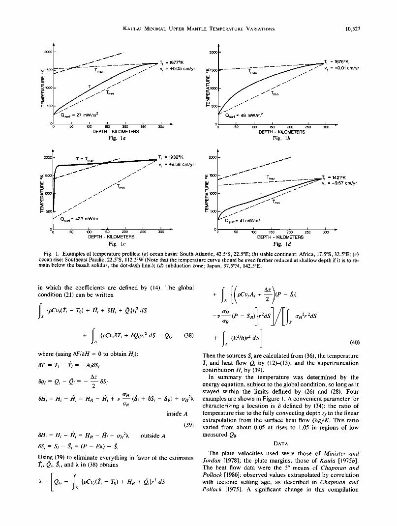
Fig. 1. Examples of temperature profiles' (a) ocean basin; South Atlantic, 42.5øS, 22.5øE ß (b) stable continent' Africa, 17.5øS, 32.5øE ß (c) ocean rise' Southeast Pacific, 22.5øS, 112.5øW (Note that the temperature curve should be even further reduced at shallow depth if it is to re- main below the basalt solidus, the dot-dash line.); (d) subduction zone; Japan, 37.5øN, 142.5øE.

in which the coefficients are defined by (14). The global condition (21) can be written

fS {pCur(• i -- TO) q- t• i q- (•H i q- Oi}ri 2 aS

+ IA {pCv,.&Ti + &Qi}ri 2 dS = Qo (38)

where (using OF/OH = 0 to obtain H•)'

aL = r,- = -AaS

Az &q/ = Qi- Oi = - --

2

an, = n,- fi, = - fi, + IT H

O' R (•i + (•Si- SR) + crn2k

inside A

(39)

alii = Hi- t•i = H• - t•i + crn2X outside A

aSi= Si- •i= (P- EX) - •i

Using (39) to eliminate everything in favor of the estimates •Pi, Oi, •i, and X in (38) obtains

X=[Qo- fs{pCvr(•'-To)+H•+Q'}r2dS

- •-- (P - S•) r2dS crH2r 2dS O'R S

+ fA (E2/h)r2 dSl (40)

Then the sources S• are calculated from (36), the temperature T• and heat flow Qi by (12)-(13), and the supertruncation contribution H• by (39).

In summary the temperature was determined by the energy equation, subject to the global condition, so long as it stayed within the limits defined by (26) and (28). Four examples are shown in Figure 1. A convenient parameter for characterizing a location is • defined by (34): the ratio of temperature rise to the fully convecting depth zf to the linear extrapolation from the surface heat flow Qoz/K. This ratio varied from about 0.05 at rises to 1.05 in regions of low measured Q0.

DATA

The plate velocities used were those of Minister and Jordan [1978]; the plate margins, those of Kaula [1975b]. The heat flow data were the 5 ø means of Chapman and Pollack [1980]: observed values extrapolated by correlation with tectonic setting age, as described in Chapman and Pollack [1975]. A significant change in this compilation

10,328 KAULA.' MINIMAL UPPER MANTLE TEMPERATURE VARIATIONS

..

-oo Deg C/My

Plate 1. Effective sources -S/pC, in øC/m.y. averaged over the uppermost 10 km. As discussed in the text, the large values arise from advection, v- VT.

...............

:!::::-:.-.:..

60 ø

•0 ø

• 300

30 ø

60 ø

0 o

--2•5o --•50 +60 +•6o +250 +1300 Deg C

Plate 2. Temperatures at 10-km depth; they are dependent almost entirely on the prescribed surface heat flow less source effects in the hottest regions.

KAULA' MINIMAL UPPER MANTLE TEMPERATURE VARIATIONS 10,329

--. "?'•- +50 +I50 +250

Deg C

Plate 3. Temperatures at 280-km depth, which are dependent on the velocity field integrated down from the surface' a mean temperature of 1676øK ' a mean heat transfer of 67 mW/m 2' expression of velocities and temperatures as 5 ø square means; and the optimization of (29) with the norm n = 2.0.

--800 2z.") 'r90 +t60 +240 +300

Deg C

Plate 4. Temperatures at 100-km depth, which are dependent on integration of the energy equation down from the surface plus limitations based on the temperatures at the fully convecting depth of 280 km.

10,330 KAULA: MINIMAL UPPER MANTLE TEMPERATURE VARIATIONS

TABLE 1. Solution Parameter Values

Parameter Defining

Symbol Equation U nit

Norm for fully convecting n (29) level

Standard Derivations

Sources •rs (32) Heat Transfer

Subtruncation •rQ (32) Supertruncation rr, (32)

Temperature rrr (32) Correlation

Sources and heat transfer •, (32) Temperature curve expo- p (35)

nent

Value(s)

1.5, 2.0, 2.5

W/m 3 1.0 x 10 -7

W/m 2 3.0 x 10 -3 W/m 2 3.0 x 10 -3

øC 30.0

0.5

1.1

between 1975 and 1980 was to increase the estimate in

regions of rapid spreading to allow for hydrothermal circula- tion at rises. The topography entered into our calculation only to define the thickness of the continental crust. The margin between continent and ocean was taken as the minimum in the hyposometric curve, about 1.5 km below sea level.

The continental crustal thickness was calculated by as- suming Airy isostasy. The continental heat source content qR followed the model of Chapman and Pollack [1975] and Pollack and Chapman [1977]. The oceanic crustal thickness was assumed to be 6 km and the heat source content qR to be 10 -7 W/m 3 (10 -6 ergs/cm3/s).

The mean temperatures and material parameters (density, thermal expansivity, thermal diffusivity, and viscosity) used were those given in Table 4 of Kaula [1980]. In addition, an intrinsic heat source density (q• - pCOT/Ot) of 2.5 x 10 -8 W/m 3 in the mantle was assumed. From a purely spatial integration, such as in this paper, there is no way to distinguish radioactive sources from cooling. Such a dis- crimination requires a temporal integration as well.

COMPUTATIONS AND RESULTS

Aside from the surface field values and material properties outlined in the previous section, there are only seven neces-

sary parameters for the model developed here. These are given in Table 1. However, of these parameters, only the fully convecting level norm exponent n was found to have a significant effect, since the others act only through the level- by-level adjustment equation (32). For the reference values S•, H•, and Q• the extrapolated estimates (24), (23), and (20) were used. For TR the smooth curve (33) was used.

Table 2 summarizes the effects of varying the fully con- vecting level norm n. The greater value of n = 2.5 leads to implausibly large temperature extremes around rises, while the lesser value of 1.5 leads to an implausibly choppy temperature pattern, in part an exaggeration of "Gibbs effects" in the velocity field. All solutions obtain a maximum temperature range of --- 1500øC at about 10-km depth, a rather unavoidable consequence of the extraordinary range from 16 to 423 mW/m 2 in observed heat flow. This temperature range is greater than is petrologically permissible, as indicated in Figure l c. Given the constraint of an adiabat to the fully convecting level, there necessarily must be an extremum of source terms S or advection--approximately -S/pC by (5) and (10)--at very shallow depth below regions of high heat flow. Most notable is the southeast Pacific Rise, where the advection must average about -200ø/m.y. in the top 10 km. (In contrast, typical oceanic crust radioactivity, -q•/pC is only - 10ø/m.y. and the mean intrinsic sources of the mantle,

TABLE 2. Summary of Solution Properties

Depth, km

Property 10 20 50 100 180 280

Temperature, øK Mean 570 770 1218 1541 1619 1676

Extremes (Relative to Mean) n = 1.5 min -213 -387 -699 -802 -528 - 178

max + 1208 +965 +532 +233 + 193 + 185

n = 2.0 min -234 -387 -700 -809 -545 -255 max + 1312 + 1048 +616 +371 +280 +274

n = 2.5 min -234 -467 -701 -809 -592 -322 max + 1319 + 1137 + 706 +407 + 373 + 369

Conducted Flow, m W/m 2 n = 2.0 min 1.3 1.1 1.2 1.5 1.9

mean 66.6 52.1 36.3 8.5 3.0 max 376.3 224.7 109.0 62.9 33.4

Convected Flow, mW/m 2 Mean 2.3 16.2 31.6 59.2 64.4

Sources, 10 -7 W/m 3 n = 2.0 min -55.5 -301.3 -38.1 -6.0 - 1.3

mean 2.1 - 1.4 -0.3 -0.0 0.0

max +88.5 +36.6 + 13.5 +6.2 + 1.0

2.0 2.4

2.7

64.8

0.0

0.0

0.0

KAULA: MINIMAL UPPER MANTLE TEMPERATURE VARIATIONS 10,331

-qR/pC + OT/Ot, are about -0.2ø/m.y.) In the formalism of this paper the large local convective heat transfer associated with partial melting, etc., must be nonlinear variation in sources S between level zi-! and level zi at which the maximum condition (28) is satisfied. From (12):

(S)i-!/2 = (Qi-! - Qi)/Az (41)

Plate 1 is a plot of these averaged sources converted to units of advection (øC/m.y.) by application of the factor -1/pC. The maximum averaged advection decreases from 190ø/m.y. in the top 10 km to 130ø/m.y. over 10-20 km depth, 50ø/m.y. over 40-50 km, 16ø/m.y. over 90-100 km, 6ø/m.y. over 180-200 km depth, etc.

Plates 2-4 give the temperatures at depths of 10 km, 280 km, and 100 km. The most implausible features in these plots, the very low temperatures --- 1000 km, of --- 15 m.y., off rapidly spreading rises, are the consequence of low observed heat flows: for example, 32 mW/m 2 at -2.5 ø latitude, 237.5 ø longitude; 34 mW/m 2 at -325 ø, 92.5 ø. These are probably the result of measurements in regions of permeable sediments where the temperature gradient is depressed by hydrother- mal circulation [Anderson et al., 1977; Sclater et al., 1980; Anderson and Skilbeck, 1981].

As discussed in the introduction, judgment as to the extent that these irregular appearing patches of low temperature are real must depend on more detailed examination of heat flow observations.

CONCLUSIONS

The fundamental premises of this paper are: 1. The velocity field to depth 280 km does not differ

significantly from an extrapolation from the surface field that takes into account only radial variation in viscosity and density.

2. Eighty-six percent of the heat flow out of the earth, 4 x 1013 W, comes from below 30 km.

3. The heat transfer at 280-km depth is entirely convec- tive.

4. The temperature gradient with respect to depth is everywhere at least adiabatic: OT/Oz -> a g T/C.

5. The surface heat flow field of Chapman and Pollack [1980] is correct.

6. The surface velocity field of Minster and Jordan [1978] is correct.

7. The material parameters and mean temperatures of Kaula [1980] are correct.

8. The temperature and velocity fields are adequately represented by 5 ø square means.

Given these premises, the following inferences seem rath- er ineluctable:

1. The greatest lateral differences in temperature, ---1500øC, occur within the top 20 km.

2. The greatest nonlinear terms in the energy equation, ---200øC/m.y., occur within the top 20 km.

3. Below ---50-km depth, the greatest departures in tem- perature from the mean are negative "tongues," which reach an extreme of about -825øC at depth ---100 km.

4. Below ---50-km depth, heat transfer is more convec- tive than conductive.

5. At the fully convecting level of---280 km, temperature variations are at least _ 180øC about the mean.

These inferences are not sensitive to the one major parameter left free by the premises, the norm n on the fully

convecting level condition, (29). The nonlinear terms more that 10ø/m.y. over the oceans must be advection, v. VT, rather than dissipation, r•k2/2pC, which for plausible strain rates averaged over •> 100 km and 3 x 10 -7 yr [Kaula, 1980] could hardly be more than 10ø/m.y. See McKenzie and Jarvis [1980] for a similar conclusion based on thermodynamic arguments.

Thus it remains to question the premises. Premise 1 implies negligible effect of shallow inhomogen-

eities on the velocity and may seem at first sight to contra- dict various force balance models involving "slab pulls," "ridge push," etc. [e.g., Forsyth and Uyeda, 1975]. Howev- er, these models are incorporated by starting from the observed surface velocities; the premise is more accurately stated as having no significant nonlinear departures from the flows inferred from the surface velocities.

Premise 2 regarding heat sources is really that 50% of the heat outside that convectively transported comes from be- low 30 km, since about 70% of the total is lost by cooling of the spreading oceanic lithosphere [Sclater et al., 1980].

Premise 3, a fully convecting level, is contrary to indica- tions of the tectosphere of Jordan [ 1979] if applied at a depth of 280 km, since at this depth there may still be perceptible conductive transfer under old continents. However, these regions are of slight contribution to the global heat budget. More serious, the implementation of the fully convecting level hypothesis at depth 280 km by the optimizing condition (29), with uniform norm n, lead to temperatures which may be too high in subduction zones (but it should be recalled that these temperatures are 5 ø block means). Application at a greater depth, however, would make premise 1 (no effect on the velocity field of lateral inhomogeneities, etc.) more wrong. A compromise might be to use a higher norm n for temperatures below the mean, T < To, than for those above.

Premise 4 regarding the limit on temperature gradients is somewhat arbitrary; it does not come from physical necessi- ty. But, as indicated by boundary layer theory [Olson and Cotcos, 1980], contradictions are of limited extent and are not inferable from more detailed examination of observa-

tions [Lewis, 1981]. In any case, their global significance is slight.

Premise 5, the correctness of the surface heat flow field, is the most questionable because of the data sparsity. Ironical- ly, the most dubious low temperatures probably arise from areas of some data, but limited and nonrepresentative (be- cause of hydrothermal circulation, etc.), rather than areas of no data at all, where the plausible extrapolation based on age and tectonic setting was used by Chapman and Pollack [1975, 1980].

Premise 6, (the velocity field) is as sure as the plate tectonic hypothesis, while Premise 7 (material parameters) is essentially a corollary of premise 1: given the kinematics, it takes an appreciable depth--more than 280 km--for physical effects to make a perceptible difference.

Premise 8 (representation by 5 ø square means) appears to be quite questionable. A harmonic analysis of the radial velocity Vr led to a rather slowly decreasing spectrum. Hence an appreciable portion of the heat transfer v,.AT could be provided by variations of shorter scale than 5 ø .

Inferences 1-4 stated above thus appear to be rather firm. But the temperature variations at the fully convecting level, _+ 180øC, may be too high.

All the inferences are adumbrated in earlier studies. The

10,332 KAULA.' MINIMAL UPPER MANTLE TEMPERATURE VARIATIONS

temperatures under stable areas, Figure l(a, b), fall within the range of earlier studies, such as Sclater et al. [1980]. The high-temperature differences and advection in the top 20 km are necessary implications of petrological studies of ocean rise conditions, such as Bottinga and Alldgre [1978], as well as more detailed geophysical analyses, such as Lewis [1981]. The temperatures about 800øC below the mean at -100-km depth occur in thermal models of subduction zones, such as Toks6z et al. [1971] and Bird [1978]. However, a global solution, although unavoidably crude, is necessary to con- nect surface-data-based crust and lithosphere models to more comprehensive mantle convection studies.

Acknowledgments. This work was supported by NASA grant NSG-5263. H. N. Pollack, University of Michigan, kindly provided the heat flow data. Helpful comments were received from N.H. Sleep, Stanford University, and two anonymous referees.

REFERENCES

Anderson, R. N., and J. N. Skilbeck, Oceanic heat flow, in The Oceanic Lithosphere, The Sea VII, edited by C. Emiliani, pp. 489-523, John Wiley, New York, 1981.

Anderson, R. N., M. G. Langseth, and J. G. Sclater, The mecha- nism of heat transfer through the floor of the Indian Ocean, J. Geophys. Res., 82, 3391-3409, 1977.

Bird, P., Stress and temperature in subduction shear zones: Tonga and Mariana, Geophys. J. R. Astron. Soc., 55,411-434, 1978.

Bottinga, Y., and C. J. All•gre, Partial melting under spreading ridges, Phil. Trans. R. Soc. Lond. A., 288, 501-525, 1978.

Chapman, D. S., and H. N. Pollack, Global heat flow: A new look, Earth Planet. Lett., 28, 23-32, 1975.

Chapman, D. S., and H. N. Pollack, Global heat flow: Degree 18 spherical harmonic representation, EOS Trans. AGU, 61, 383, 1980.

Embley, R. W., M. A. Hobart, R. N. Anderson, and D. Abbott, Anomalous heat flow in the northwest Atlantic: A case for

continued hydrothermal circulation in 80-m.y. crust, J. Geophys. Res., 88, 1067-1074, 1983.

Forsyth, D., and S. Uyeda, On the relative importance of the driving forces of plate motion, Geophys. J. R. Astron. Soc., 43, 163-200, 1975.

Hager, B., and R. J. O'Connell, Subduction zone dip angles and flow driven by plate motion, Tectonophysics, 50, 111-138, 1978.

Hager, B., and R. J. O'Connell, Kinematic models of large-scale flow in the earth's mantle, J. Geophys. Res., 84, 1031-1048, 1979.

Hager, B., and R. J. O'Connell, A simple global model of plate dynamics and mantle convection, J. Geophys. Res., 86, 4843- 4867, 1981.

Jordan, T. H., The deep structure of the continents, Sci. Am., 240(1), 92-107, 1979.

Kaula, W. M., Product-sum conversion of spherical harmonics with application to thermal convection, J. Geophys. Res., 80, 225-231, 1975a.

Kaula, W. M., Absolute plate motions by boundary velocity minimi- zations, J. Geophys. Res., 80, 244-248, 1975b.

Kaula, W. M., Extensions of the theory of statistical analysis on a sphere, Boll. Geod. Sci. Aft., 37, 495-505, 1978.

Kaula, W. M., Material properties for mantle convection consistent with observed surface fields, J. Geophys. Res., 85, 7031-7044, 1980.

Lewis, B. T. R., Isostasy, magma chambers, and plate driving forces on the East Pacific Rise, J. Geophys. Res., 86, 4868-4880, 1981.

McKenzie, D. P., and G. Jarvis, The conversion of heat into mechanical work by mantle convection, J. Geophys. Res., 85, 6093-6096, 1980.

McKenzie, D. P., M. J. Roberts, and N. O. Weiss, Convection in the earth's mantle: Toward a numerical simulation, J. Fluid Mech., 62,465-538, 1974.

Minister, J. B., and T. H. Jordan, Present-day plate motions, J. Geophys. Res., 83, 5331-5334, 1978.

Olson, P., and G. M. Corcos, A boundary layer model for mantle convection with surface plates, Geophys. J. R. Astron. Soc., 62, 195-219, 1980.

Pollack, H. N., and D. S. Chapman, On the regional variations of heat flow, geotherms, and lithospheric thickness, Tectonophy- sics., 38, 279-296, 1977.

Sclater, J. G., C. Jaupart, and D. Galson, The heat flow through oceanic and continental crust and the heat loss of the earth, Rev. Geophys. Space Phys., 18, 264-311, 1980.

Sclater, J. G., B. Parsons, and C. Jaupart, Oceans and continents: Similarities and differences in the mechanisms of heat loss, J. Geophys. Res., 86, 11,535-11,552, 1981.

Toks6z, M. N., J. W. Minear, and B. R. Julian, Temperature field and geophysical effects of a downgoing slab, J. Geophys. Res., 76, 1113-1138, 1971.

W. M. Kaula, Department of Earth and Space Sciences, Universi- ty of California, Los Angeles, CA 90024.

(Received April 2, 1982; revised June 7, 1983;

accepted June 15, 1983.)