JOURNAL OF LATEX CLASS FILES, VOL. XX, NO. XX, SEPTEMBER 2019 1

PID Controller based Stochastic OptimizationAcceleration for Deep Neural Networks

Haoqian Wang, Yi Luo, Wangpeng An, Qingyun Sun,Jun Xu, Yongbing Zhang, Yulun Zhang, and Lei Zhang, Fellow, IEEE

Abstract—Deep neural networks (DNNs) are widely used anddemonstrated their power in many applications, like computervision and pattern recognition. However, the training of these net-works can be time-consuming. Such a problem could be alleviatedby using efficient optimizers. As one of the most commonly usedoptimizers, SGD-Momentum uses past and present gradientsfor parameter updates. However, in the process of networktraining, SGD-Momentum may encounter some drawbacks, suchas the overshoot phenomenon. This problem would slow thetraining convergence. To alleviate this problem and acceleratethe convergence of DNN optimization, we propose a proportional-integral-derivative (PID) approach. Specifically, we investigate theintrinsic relationships between PID based controller and SGD-Momentum firstly. We further proposed a PID based optimizationalgorithm to update the network parameters, where the past,current, and change of gradients are exploited. Consequently,our proposed PID based optimization alleviates the overshootproblem suffered by SGD-Momentum. When tested on popularDNN architectures, it also obtains up to 50% acceleration withcompetitive accuracy. Extensive experiments about computervision and natural language processing demonstrate the effective-ness of our method on benchmark datasets, including CIFAR10,CIFAR100, Tiny-ImageNet, and PTB. We’ve released the code athttps://github.com/tensorboy/PIDOptimizer.

Index Terms—Deep neural network, optimization, PID control,SGD-Momentum.

I. INTRODUCTION

Benefitting from the availability of great number of data(e.g., ImageNet [1]) and the fast-growing power of GPUs, deepneural networks (DNNs) success in a wide range of applica-tions, like computer vision and natural language processing.Despite the significant successes of DNNs, the training andinference of deep and wide DNNs are often computationallyexpensive, which may take several days or longer even withpowerful GPUs. Many stochastic optimization algorithms are

This work is partially supported by the NSFC fund (61571259, 61831014,61531014), in part by the Shenzhen Science and Technology Project underGrant (GGFW2017040714161462, JCYJ20170307153051701). (Correspond-ing author: Y. Zhang, Email: zhang.yongbing@sz.tsinghua.edu.cn.)

H. Wang, Y. Luo, W. An, and Y. Zhang are with the GraduateSchool at Shenzhen, Tsinghua University, and also with Shenzhen Insti-tute of Future Media Technology, Shenzhen 518055, China. E-mail: wang-haoqian@tsinghua.edu.cn, vast2stars@gmail.com, anwangpeng@gmail.com,zhang.yongbing@sz.tsinghua.edu.cn.

Q. Sun is with Department of Mathematics, Stanford University, Stanford,CA 94305. E-mail: qysun@stanford.edu.

J. Xu is with College of Computer Science, Nankai University, Tianjin300071, China. E-mail: nankaimathxujun@gmail.com.

Y. Zhang is with Department of ECE, Northeastern University, Boston, MA02115. E-mail: yulun100@gmail.com.

L. Zhang is with Department of Computing, the Hong Kong PolytechnicUniversity, Hong Kong, and also with the Artificial Intelligence Center,Alibaba DAMO Academy. Email: cslzhang@comp.polyu.edu.hk.

not only used in the field of machine learning [2], but alsodeep learning [3]. It is very important to explore how to boostthe speed of training DNNs while maintaining performance.Furthermore, with a better optimization method, even a com-putation limited hardware (e.g., IoT device) can save lots oftime and memory usage. The accelerating methods of thecomputational time for DNNs can be divided into two parts,the speed-up of training and that of test. The methods in [4]–[6] aiming to speed up test process of DNNs often focus onnot only the decomposition of layers but also the optimizationsolutions to the decomposition. Besides, there has been otherstreams on improving testing performance of DNNs, such asthe FFT-based algorithms [7] and reduced parameters in deepnets [8]. As for the methods to speed up the training speedof DNNs, the key factor is the way to update the millionsof parameters of a DNN. This process mainly depends onoptimizer and the choice of optimizer is also a key point of amodel. Even with the same dataset and architecture, differentoptimizers could result in very different training effects, due todifferent directions of the gradient descent, different optimizersmay reach completely different local minimum [9].

The learning rate is another principal hyper-parameter forDNN training [10]. Based on different strategies of choosinglearning rates, DNN optimizers can be categorized into twogroups: 1. Hand-tuned learning rate optimizers: stochastic gra-dient descent (SGD) [11], SGD Momentum [12], Nesterov′sMomentum [12], etc. 2. Auto learning rate optimizers such asAdaGrad [13], RMSProp [14] and Adam [15], etc.

The SGD-Momentum method puts past and current gra-dients into consideration and then updates the network pa-rameters. Although SGD-Momentum performs well in mostcases, it may encounter overshoot phenomenon [16], whichindicates the case where the weight exceeds its target valuetoo much and fails to correct its update direction. Such anovershoot problem costs more resource (e.g., time and GPUs)to train a DNN and also hampers the convergence of SGD-Momentum. So, a more efficient DNN optimizer is eagerlydesired to alleviate the overshoot problem and achieve betterconvergence.

The similarity between optimization algorithms popularlyemployed in DNN training and classic control methods hasbeen investigated in [17]. In automatic control systems, thefeedback control is essential. Proportional-integral-derivative(PID) controller is the most widely used feedback controlmechanism, due to its simplicity and functionality [18]. Mostof industrial control system are based on PID [19], such asunmanned aerial vehicles [20], robotics [21], and autonomous

JOURNAL OF LATEX CLASS FILES, VOL. XX, NO. XX, SEPTEMBER 2019 2

vehicles [22]. PID control takes current error, change inerror (differentiation of the error over time), and the pastcumulative error (integral of the error over time) into account.So, the difference between current and expected outputs willbe minimized.

On the other hand, few studies have been done on theconnections between PID with DNN optimization. In thiswork, we investigate specific relationships analytically andmathematically towards this research line. We first clarifythe intrinsic connection between PID controller and stochasticoptimization methods, including SGD, SGD-Momentum, andNesterov′s Momentum. Finally, we propose a PID basedoptimization method for DNN training. Similar to SGD-Momentum, our proposed PID optimizer also considers thepast and current gradients for network update. The LaplaceTransform [23] is further introduced for hyper-parameter ini-tialization, which makes our method simple yet effective. Ourmajor contributions of this work can be summarized in threefolds:

• By combining the error calculation in the feedback con-trol system with network parameters’ update, we reveala potential relationship between DNN optimization andfeedback system control. We also find that some opti-mizers (e.g., SGD-Momentum) are special cases of PIDcontrol device.

• We propose a PID based DNN optimization approachby taking the past, current, and changing informationof the gradient into consideration. The hyper-parameterin our PID optimizer is initialized by classical LaplaceTransform.

• We systematically experiment with our proposed PIDoptimizer on CIFAR10, CIFAR100, Tiny-ImageNet, andPTB datasets. The results show that PID optimizer isfaster than SGD-Montum in DNN training process.

A preliminary version of this work was presented as aconference version [24]. In the current work, we incorporateadditional contents in significant ways:

• We evaluate the performance of our PID optimizer on thelanguage modeling application by utilizing the character-level Penn Treebank (PTB-c) dataset with an LSTMnetwork.

• The proposed PID optimizer is applied on GAN withMNIST dataset and show the digital images generatedby them separately to illustrate that our method is alsoapplicable in GAN.

• We update the conclusion that the proposed PID optimizerexceeds SGD-Momentum in GANs and RNNs.

We organize the rest of this paper as follows. Section IIbriefly surveys related works. Section III investigates therelationship between PID controller and DNN optimization al-gorithms. Section IV introduces the proposed PID approach forDNN optimization. Experimental results and detailed analysisare reported in Section V. Section VI concludes this paper.

II. RELATED WORKS

A. Classic Deep Neural Network Architectures

CNN. Convolutional neural networks (CNNs) [25] haverecently achieved great successes in visual recognition tasks,including image classification [26], object detection [27]–[29], and scene parsing [30]. Recently, lots of deep CNNarchitectures, such as VGG, ResNet, and DenseNet, have beenproposed to improve the performance of these tasks mentionedabove. Network depth tends to improve network performance.However, the computational cost of these deep networks alsoincreases significantly. Moreover, real-world systems may beaffected by the high cost of these networks.

GAN. Goodfellow et al. firstly proposed generative ad-versarial network (GAN) [31], which consists of generativeand adversarial networks. The generator tries to obtain veryrealistic outputs to foolish the discriminator, which wouldbe optimized to distinguish between the real data and thegenerated outputs. GANs will be trained to generate syntheticdata, mimicking genuine data distribution.

In machine learning, models can be classified into twocategories: generative model and discriminative model. A dis-criminative network (denoted as D) can discriminate betweentwo (or more) different classes of data, such as CNN trainedfor image classification. A generative network (denoted asG) can generate new data, which fit the distribution of thetraining data. For example, a trained Gaussian Mixture Modelis able to generate new random data, which more-or-less fitthe distribution of the training data.

GANs pose a challenging optimization problem due tothe multiple loss functions, which must be optimized simul-taneously. The optimization of GAN is conducted by twosteps: 1) optimize discriminative network while fixing thegenerative one. 2) optimize the generative network whilefixing the discriminative network. Here, fixing a networkmeans only allowing the network to pass forward and notperform back-propagation. These two steps are seamlesslyalternating updated and dependent on each other for efficientoptimization. After enough training cycles, the optimizationobjective V (D,G) introduced in [31] will reach the situation,where the probability distribution of the generator exactlymatches the true probability distribution of the training data.Meanwhile, the discriminator has the capability to distinguishthe realistic data from the virtual generated ones. However, theperfect cooperation between the generator and discriminatorwill fail occasionally. The whole system will reach the statusof “model collapse”, indicating that the discriminator and thegenerator tend to produce the same outputs.

LSTM. Hochreiter et al. firstly proposed the Long ShortTerm network, generally called LSTM, to obtain long-termdependency information from the network. As a type ofrecurrent neural network (RNN), LSTM has been widelyused and obtained excellent success in many applications.LSTM is deliberately designed to avoid long-term dependencyproblems. Remember that long-term information is the defaultbehavior of LSTM in practice, rather than the ability to acquireat great cost. All RNNs have a chained form of repeatingnetwork modules. In the standard RNN, this repeating module

JOURNAL OF LATEX CLASS FILES, VOL. XX, NO. XX, SEPTEMBER 2019 3

often has a simple structure (e.g., “tanh” layer). The outputsof all LSTM cells are utilized to construct a new feature,where multinomial logistic regression is introduced to formthe LSTM model.

One widely used way to evaluate RNN models is the addingtask [32], [33], which takes two sequences of length T as input.By sampling in the range (0,1) uniformly, we form the firstsequence. For another sequence, we set two entries as 1 andthe rest as 0. The output is obtained by adding two entries inthe first sequence. The positions of the entries are determinedby the two entries of 1 from the second sequence.

B. Accelerating the Training/Test Process of DNNs

Training process acceleration. Since DNNs are mostlycomputationally intensive, Han et al. [34] proposed a deepcompression method to reduce the storage requirement ofDNNs by 35× to 49× without affecting the accuracy. More-over, the compressed model has 3× to 4× layer-wise speedupand 3× to 7× better energy efficiency. Unimportant connec-tions are pruned. Weight sharing and Huffman coding areapplied to quantize the network. This work mainly attemptsto reduce the number of parameters of neural networks. Liuet al. proposed the network slimming technique that cansimultaneously reduce the model size, running-time mem-ory, and computing operations [35]. Yang et al. proposed anew filter pruning strategy based on the geometric medianto accelerate the training of deep CNNs [36]. Dai et al.proposed a synthesis tool to synthesize compact yet accurateDNNs [37]. Du et al. proposed a Continuous Growth andPruning (CGaP) scheme to minimize the redundancy fromthe beginning [38]. Hubara et al. introduced a method totrain Quantized Neural Networks that reduce memory sizeand accesses during forward pass [39]. In [40], Han et al.presented an intuitive and easier-to-tune version of ASGD(please refer to Section IV) and showed that ASGD leads tofaster convergence significantly with a comparable accuracythan SGD, Heavy Ball, and Nesterov′s Momentum [12].

Test process acceleration. Denton et al. [4] proposeda method that compresses all convolutional layers. This isachieved by approximating proper low-rank and then updat-ing the upper layers until the prediction result is enhanced.Based on singular value decompositions (SVD), this processconsists of numerous tensor decomposition operations andfilter clustering approaches to make use of similarities amonglearned features. Jaderberg et al. [5] introduced an easy-to-implement method that can significantly speed up pretrainedCNNs with minimal modifications to existing frameworks.There can be a small associated loss in performance, butthis is tunable to a desired accuracy level. Zhang et al. [6]first proposed a response reconstruction method, which in-troduces the nonlinear neurons and a low-rank constraint.Without the usage of SGD and based on generalized singularvalue decomposition (GSVD), a solution is developed for thisnonlinear problem. Li et al. presented a method to prunefilters with relatively low weight magnitudes to produce CNNswith reduced computation costs without introducing irregularsparsity [41].

C. Deep Learning Optimization

In the training of DNN [10], learning rate is an essentialhyper-parameter. DNN optimizers can be categorized into twogroups based on different strategies of setting the learningrate: 1. Hand-tuned learning rate optimizers: stochastic gra-dient descent (SGD) [11], SGD Momentum [12], Nesterov′sMomentum [12], etc. 2. Auto learning rate optimizers, such asAdaGrad [13], RMSProp [14], and Adam [15], etc. Good re-sults have been achieved on CIFAR10, CIFAR100, ImageNet,PASCAL VOC, and MS COCO datasets. They were mostlyobtained by residual neural networks [42]–[45] trained by us-ing SGD-Momentum. This work focuses on the improvementof the fist category of optimizers. The introduction to theseoptimizers is as follows.

Classical Momentum [25] is the first ever variant of gradientdescent involving the usage of a momentum parameter. In theobjective across iterations, it accelerates gradient descent thatcollects a velocity vector in directions of continuous reduction.

Stochastic Gradient Descent (SGD) [11] is a widely usedoptimizer for DNN training. SGD is easy to apply, but thedisadvantage of SGD is that it converges slowly and mayoscillate at the saddle point. Moreover, how to choose thelearning rate reasonably is a major difficulty of SGD.

SGD Momentum (SGD-M) [12] is an optimization methodthat considers momentum. Compared to the original gradientdescent step, the SGD-M introduces variables related to theprevious step. It means that the parameter update directionis decided not only by the present gradient, but also by thepreviously accumulated direction of the fall. This allows theparameters to change little in the direction where gradientchange frequently. Contrary to this, SGD-M changes parame-ters a lot in the direction where gradient change slowly.

Nesterov′s Momentum [12] is another momentum optimiza-tion algorithm motivated by Nesterov′s accelerated gradientmethod [46]. Momentum is improved from the SGD algorithm,so that each parameter update direction depends not only onthe gradient of the current position, but also on the directionof the last parameter update. In other words, Nesterov′s Mo-mentum essentially uses the second-order information of theobjective (loss function) so it can accelerate the convergencebetter.

D. PID Controller

Traditionally, the PID controller has been used to controla feedback system [19] by exploiting the present, past, andfuture information of prediction error. The theoretical basis ofthe PID controller was first proposed by Maxwell in 1868in his seminal paper “On Governors” [47]. Mathematicalformulation was given by Minorsky [48]. In recent years,several advanced control algorithms have been proposed.

We define the difference between the actual output and thedesired output as error e(t). The PID controller calculates theerror e(t) in every step t, and then applies a correction u(t)to the system as a function of the proportional (P), integral

JOURNAL OF LATEX CLASS FILES, VOL. XX, NO. XX, SEPTEMBER 2019 4

Update

Devices

Desired Value

PID Controller Output

Feedback

Error

Loss L

Backpropagation

𝜕𝐿

𝜕𝑤𝑖𝑗

𝜕𝐿

𝜕𝑤𝑗𝑘

𝜕𝐿

𝜕𝑤𝑘𝑙

𝑤𝑘𝑙

𝑤𝑗𝑘𝑤𝑖𝑗𝑥0

𝑥3

𝑥2

𝑥1

SGD-Momentum

Update

Desired Value (Label)

Output

𝜃 = 𝑤𝑖𝑗,𝑤𝑗𝑘,𝑤𝑘𝑙

Deep Model

Training

Connection

Control

System

Fig. 1. Illustrations about the relationships between control system and deep model training. It also shows the connection between PID controller andSGD-Momentum.

(I), and derivative (D) terms of e(t). Mathematically, the PIDcontroller can be described as

u(t) = Kpe(t)+Ki

∫ t

0e(t)dt +Kd

ddt

e(t), (1)

where Kp, Ki, and Kd correspond to the gain coefficients ofthe P, I, and D terms, respectively. The function of error e(t)is the same as the gradient in optimization of deep learning.The coefficients Kp, Ki, and Kd reflect the contribution tothe current correction to the current, past, and future errorsrespectively.

According to our analyses, we find that PID control tech-niques can be more useful for optimization of deep network.The study presented in this paper is one of the first inves-tigations to apply PID as a new optimizer to deep learningfield. Our studies have succeeded in demonstrating significantadvantages of the proposed optimizer. With the inheritanceof the advantages of PID controller, the proposed optimizerperforms well despite its simplicity.

III. PID AND DEEP NEURAL NETWORK OPTIMIZATION

We reveal the intrinsic relation between PID control andDNNs optimization. The intrinsic relation inspires us to ex-plore new DNNs optimization methods. The core idea of thissection is to regard the parameter update in DNNs trainingprocess as using PID controller in the system to reach anequilibrium.

A. Overall Connections

At first, we summarize the training process of deep learning.Deep neural networks (DNNs) need to map the input x to theoutput y though parameters θ . To measure the gap betweenthe DNN output and desired output, the loss function L isintroduced. Given some training data, we can calculate the lossfunction L(θ ,Xtrain). In order to minimize the loss function L,we find the derivative of the loss function L with respect to theparameter θ and update θ with the gradient descent methodin most cases. DNNs gradually learn the complex relationshipbetween input x and output y by constantly updating theparameters θ , which called DNN’s training. The updating of θ

is driven by the gradient of loss function until it’s converged.Then, the purpose of an automated control system is to eval-

uate the system status and make it to the desired status througha controller. In feedback control system, the controller’s actionis affected by the system’s output. The error e(t) betweenthe measured system status and desired status is taken intoconsideration, so that controller can make system get close todesired status.

More specifically, as shown in Eq. (1), PID controllerestimates a control variable u(t) by considering the current,past, and future (derivative) of the error e(t).

From here we can see that the error in the PID controlsystem is related to the gradient in the deep neural networktraining process. The update of parameters during deep neuralnetwork (DNNs) training can be analogized to the adjustmentof the system by the PID controller.

JOURNAL OF LATEX CLASS FILES, VOL. XX, NO. XX, SEPTEMBER 2019 5

As can be seen from the discussion above, there is highsimilarity between DNNs optimization and PID based controlsystem. Fig. 1 shows their flowchart respectively and we cansee the similarity more intuitively. Based on the differencebetween the output and target, both of them change the sys-tem/network. The negative feedback process in PID controlleris similar as the back-propagation in DNNs optimization.

One key difference is that the PID controller computes theupdate utilizing system error e(t). However, DNN optimizerdecides the updates by considering gradient ∂L/∂θ . Let’s re-gard the gradient ∂L/∂θ as the incarnation of error e(t). Then,PID controller could be fully related with DNN optimiza-tion. In the next, we prove that SGD, SGD-Momentum andNesterov′s Momentum all are special cases of PID controller.

B. Stochastic Gradient Descent (SGD)

In DNN training, there are widely used optimizers, such asSGD and its variants. The parameter update rule of SGD fromiteration t to t +1 is determined by

θt+1 = θt − r∂Lt/∂θt , (2)

where r is the learning rate. We now regard the gradient∂Lt/∂θt as error e(t) in PID control system. Comparing withPID controller in Eq. (1), we find that SGD can be viewed asone type of P controller with Kp = r.

C. SGD-Momentum

SGD-Momentum is faster than SGD to train a DNN, be-cause it can use history gradient. The rule of SGD-M updatingparameter is given by{

Vt+1 = αVt − r∂Lt/∂θt

θt+1 = θt +Vt+1, (3)

where Vt is a term that accumulates historical gradients. α ∈(0,1) is the factor that balances the past and current gradients.It is usually set to 0.9 [49]. Dividing two sides of the 1stformula of Eq. (3) by α t+1

Vt+1

α t+1 =Vt

α t − r∂Lt/∂θt

α t+1 . (4)

By applying Eq. (4) from time t +1 to 1, we have

Vt+1

α t+1 −Vt

α t =−r∂Lt/∂θt

α t+1Vt

α t −Vt−1

α t−1 =−r∂Lt−1/∂θt−1

α t...

V1

α1 −V0

α0 =−r∂L0/∂θ0

α1 .

(5)

By adding the aforementioned equations together, we get

Vt+1

α t+1 =V0

α0 − rt

∑i=0

∂Li/∂θi

α i+1 . (6)

To make it more general, we set the initial condition V0 = 0,and thus the above equation can be simplified as follows

Vt+1 =−rt

∑i=0

αt−i

∂Li/∂θt−1. (7)

Put Vt+1 into the 2nd formula of Eq. (3), we have

θt+1−θt =−r∂Lt

∂θt− r

t−1

∑i=0

αt−i

∂Li/∂θi. (8)

We could learn that parameter update process considers boththe current gradient (P control) and the integral of pastgradients (I control). If we assume α = 1, we get followingequation

θt+1−θt =−r∂Lt/∂θt − rt−1

∑i=0

∂Li/∂θi. (9)

Comparing Eq. (9) with Eq. (1), we can see that SGD-Momentum is a PI controller with Kp = r and Ki = r. Byusing some mathematical skill [50], we simplify Eq. (3) byremoving Vt . Then, Eq. (9) can be rewritten as

θt+1 = θt − r∂Lt/∂θt − rt−1

∑i=0

∂Li/∂θiαt−i. (10)

We can see it clear that the network parameter update dependson both current gradient r∂Lt/∂θt and the integral of pastgradients r ∑

t−1i=0 ∂Li/∂θiα

t−i. It should be noted that the Iterm includes a decay factor α . Due to the huge number oftraining data, it’s better to calculate the gradient based on mini-batch of training data. So, the gradients behave in a stochasticmanner. The purpose of the introduction of decay term α isto keep the gradients away from current value, so that it canalleviate noise. In all, based on the analyses, we can viewSGD-Momentum as a PI controller.

D. Nesterov′s Momentum

Momentum is improved from the SGD algorithm and itconsiders the second-order information of the objective (lossfunction), so it can accelerate the convergence better. We setthe update rule as{

Vt+1 = αVt − r∂Lt/∂ (θt +αVt)

θt+1 = θt +Vt+1.(11)

By using a variable transform θt = θt +αVt , and formulatingthe update rule with respect to θ , we have{

Vt+1 = αVt − r∂Lt/∂ θt

θt+1 = θt +(1+α)Vt+1−αVt .(12)

Similar to the derivation process in Eq. (4)-(6) of SGD-Momentum, we have

Vt+1 =−r(t

∑i=1

(α t−i∂Li/∂ θi)). (13)

With Eq. (13), Eq. (11) can be rewritten as

θt+1− θt =− r(1+α)∂Lt/∂ θt −αr(t−1

∑i=1

(α t−i∂Li/∂ θi)).

(14)

JOURNAL OF LATEX CLASS FILES, VOL. XX, NO. XX, SEPTEMBER 2019 6

We could conclude that the network parameter update consid-ers the current gradient (P control) and the integral of pastgradients (I control). If we assume α = 1, then

θt+1− θt =−2r(∂Lt/∂ θt)− r(t−1

∑i=0

(∂Li/∂ θi)). (15)

Comparing Eq. (15) with Eq. (1), we can prove that Nesterov′sMomentum is a PI controller with Kp = 2r and Ki = r.What’s more, compared with SGD-Momentum, the Nesterov′sMomentum would utilize the current gradient and integral ofpast gradients to update the network parameters, but achieveslarger gain coefficient Kp.

IV. PID BASED DNN OPTIMIZATION

A. The Overshoot Problem of SGD-Momentum

We can learn it from Eqs. (10) and (14) that the Momentumoptimizer will accumulate history gradients to accelerate. Buton the other hand, the updating of parameters may be in wrongpath, if the history gradients lag the update of parameters.According to the definition “the maximum peak value of theresponse curve measured from the desired response of the sys-tem” in discrete-time control systems [16], this phenomenonis named as overshoot. Specifically, it can be written as

Overshoot =θmax−θ ∗

θ ∗, (16)

where θmax and θ ∗ are the maximum and optimum values ofthe weight, respectively.

The overshoot problem’s test benchmark is the first functionof De Jong′s [51] due to its smooth, unimodal, and symmetriccharacteristics. The function can be written as

f (x) = 0.1x21 +2x2

2, (17)

whose search domain is −10≤ xi ≤ 10, i = 1,2. For this func-tion x∗ = (0,0), f (x∗) = 0, we can pursue a global minimumrather then a local one.

To build a simple PID optimizer, we introduce a derivativeterm of gradient based on SGD-Momentum

PID = Momentum+Kd(∂ f (x)/∂xc−∂ f (x)/∂xc−1), (18)

where c is the present iteration index for x. With differentchoices of Kd in Eq. (18), we shows the results of simulationin Fig. 2, where the loss-contour map is represented as thebackground. The redder, the bigger the loss function value is.In contrast, the bluer, the smaller the loss function value is.The x-axis and y-axis denote x1 and x2, respectively. Both x1and x2 are initialized to −10. We use red and yellow linesto show the path of PID and SGD-Momentum, respectively.It is obvious that SGD-Momentum optimizer suffers fromovershoot problem. By increasing Kd gradually (0.1, 0.5, and0.93, respectively), our PID optimizer uses more “future”error, so that it can largely alleviate the overshoot problem.

B. PID Optimizer for DNN

We are motivated by the simple example in Section IV-Aand seek a PID optimizer to boost the convergence of DNNtraining. From Eq. (10), SGD-Momentum can be viewed asa PI controller, which takes current and past gradient infor-mation actually. Fig. 2 shows that PID controller introduces aderivative term of gradient to use the future information. Then,the overshoot problem can be alleviated obviously.

On the other hand, it is very easy to introduce noise whencomputing of gradients, because the training is often conductedin a mini-batch manner. We also try to estimate the averagemoving of the derivative part. Our proposed PID optimizerupdates network parameter θ in iteration (t +1) by

Vt+1 = αVt − r∂Lt/∂θt

Dt+1 = αDt +(1−α)(∂Lt/∂θt −∂Lt−1/∂θt−1)

θt+1 = θt +Vt+1 +KdDt+1.

(19)

We could learn from Eq. (19) that a hyper-parameter Kd isintroduced in the proposed PID optimizer. We initialize Kdby introducing Laplace Transform [23] theory and Ziegler-Nichols [52] tuning method.

C. Initialization of Hyper-parameter Kd

The Laplace Transform converts the function of real variablet to a function of complex variable s. The most commonusage is to convert time to frequency. Denote the Laplacetransformation of f (t) as F(s). There is

F(s) =∫

∞

0e−st f (t)dt, for s > 0. (20)

In general, it’s easier to solve F(s) than f (t), which can bereconstructed from F(s) with the Inverse Laplace transform

f (t) =1

2πilim

T→∞

∫γ+iT

γ−iTestF(s)ds, (21)

where i is the unit of imagery part and γ is a real number.By using Laplace Transform, we can first transform our

PID optimizer into its Laplace transformed functions of s, andthen simplify the algebra. After obtaining the transformationF(s), we can achieve the desired solution f (t) with the inversetransform.

We initialize a parameter of a node in DNN model as ascalar θ0. After enough times of updates, the optimal value θ ∗

can be obtained. We simplify the parameter update in DNNoptimization as one step response (from θ0 to θ ∗) in controlsystem. We introduce the Laplace Transform to set Kd anddenote the time domain change of weight θ as θ(t).

The Laplace Transform of θ ∗ is θ∗s [53]. We denote by

θ(t) the weight at iteration t. The Laplace Transform of θ(t)is denoted as θ(s), and that of error e(t) as E(s),

E(s) =θ ∗

s−θ(s).

The Laplace transform of PID [53] is

U(s) = (Kp +Ki1s+Kds)E(s). (22)

JOURNAL OF LATEX CLASS FILES, VOL. XX, NO. XX, SEPTEMBER 2019 7

10.0 7.5 5.0 2.5 0.0 2.5 5.0 7.510.0

7.5

5.0

2.5

0.0

2.5

5.0

7.5

Small Kd

10.0 7.5 5.0 2.5 0.0 2.5 5.0 7.510.0

7.5

5.0

2.5

0.0

2.5

5.0

7.5

Moderate Kd

10.0 7.5 5.0 2.5 0.0 2.5 5.0 7.510.0

7.5

5.0

2.5

0.0

2.5

5.0

7.5

Big Kd

Fig. 2. The overshoot problem of momentum with different values of Kd . The red and yellow lines indicate the results obtained by PID and SGD-Momentumrespectively.

In our case, the u(t) corresponds to the update of θ(t). So wereplace U(s) with θ(s), and with E(s) = θ∗

s −θ(s). Eq. (22)can be rewritten as

θ(s) = (Kp +Ki1s+Kds)(

θ ∗

s−θ(s)). (23)

With this form, it is easy to derive a standard closed looptransfer function [54] as

θ ∗

s−θ(s) =

1Kd

ω2n

s2 +2ζ ωns+ω2n, (24)

where {Kp+1Kd

= 2ζ ωnKiKd

= ω2n .

(25)

Eq. (24) can be rewritten as

θ ∗

s−θ(s) =

(s+ζ ωn)+ζ√

1+ζ 2ωn

√1−ζ 2

(s+ζ ωn)2 +ω2n (1−ζ 2)

. (26)

We can get the time (iteration) domain form of θ(s) byusing the Inverse Laplace Transform table [53] and the initialcondition of the θ (θ0):

θ(t) = θ∗− (θ ∗−θ0)sin(ωn

√1−ζ 2t + arccos(ζ ))

eζ ωnt√

1−ζ 2(27)

and {(Kp +1)/Kd = 2ζ ωn

Ki/Kd = ω2n ,

(28)

where ζ is damping ratio and ωn is natural frequency of thesystem. The evolution process of a weight as an example ofθ(t) is shown in Fig. 3. From Eq. (28), we get

Ki =(Kp +1)2

4Kdζ. (29)

From Eq. (29) we know that Ki is a monotonically decreas-ing function of ζ . Based on the definition of overshoot in

tmax

θ0

θ∗

θmax

t

θ(t)

Fig. 3. The evolution process of the weight θ(t) for PID optimizer.

Eq. (16), it is obvious that ζ is monotonically decreasing withovershoot. Then, Ki is a monotonically increasing function ofovershoot. In a word, the more history error (Integral part),the more overshoot problem in the system. This is a goodexplanation of why SGD-Momentum overshoots its target andneed more training time.

By differentiating θ(t) w.r.t. time t, and let

dθ(t)dt

= 0.

We have the peak time of the weight as

tmax =π

wn√

1−ζ 2. (30)

Put tmax to Eq. (27), we have θmax, and put θmax to Eq. (16),we have

Overshoot =θ(tmax)−θ ∗

θ ∗= e

−ζ π√1−ζ 2

. (31)

We could learn from Eq. (27) that the term sin(ωn√

1−ζ 2t+arccos(ζ )) brings periodically oscillation change to the weight,which is no more than 1. The term e−ζ ωnt mainly controls the

JOURNAL OF LATEX CLASS FILES, VOL. XX, NO. XX, SEPTEMBER 2019 8

convergence rate. It should be noted that the value of hyper-parameter Kd in calculating the derivate

e−ζ ωn = e−Kp+12Kd . (32)

Based on the above analyses, we know that the training ofDNN can be accelerated by using large derivate. But on theother hand, if Kd is too large, the system will be fragile. Aftersome experiments, we set the Kd based on the Ziegler-Nicholsoptimum setting rule [52].

According to the Ziegler-Nichols′ rule, the ideal setup ofKd should be one third of the oscillation period (T ), whichmeans Kd = 1

3 T . From Eq. (27), we can get T = 2π

ωn√

1−ζ 2. If

we make a simplification that the α in Momentum is equal to1, then Ki = Kd = r. Combined with Eq. (28), Kd will have aclosed form solution

Kd = 0.25r+0.5+(1+169

π2)/r. (33)

For real-world cases, where different DNNs are applied trainon different datasets, we would firstly start with this idealsetting of Kd and change it slightly latter.

V. EXPERIMENTAL RESULTS

We introduce four commonly used datasets for the experi-ments. Then, we compare our proposed optimizer with otheroptimizers by using CNN and LSTM on four commonly useddatasets. Specifically, we first train an multilayer perceptron(MLP) on the MNIST dataset to demonstrate the advantagesof PID optimizer. We then train CNNs on the CIFAR datasetsto show that our PID optimizer achieves competitive accuracycompared with other optimizers, but it has a faster trainingspeed. Further studies are carried out to prove that our PIDoptimizer also performs well on a larger dataset. Based onthe Tiny-ImageNet dataset [55], we carry out a series ofexperiments. The results indicate that it is applicable forour PID optimizer to be extended to modern networks. Ourproposed PID optimizer is set to use all hyper-parameters thatare detailed for SGD-Momentum. The initial learning rate andlearning rate schedule vary with different experiments.

A. Datasets

MNIST Dataset. The MNIST dataset [56] of handwrittennumbers from 0 to 9. Being a subset of a larger dataset NIST,MNIST consists of 60,000 training data and 10,000 test ones.The digits have been size-normalized and centered in a fixed-size image of 28×28 pixels. With the usage of anti-aliasingtechnique, the preprocessed images contain gray levels.

CIFAR Datasets. The CIFAR10 dataset [57] has 60,000RGB color images, the shape of which is 32×32. There are10 classes, each of which includes 6,000 images. 50,000 and10,000 images are used for training and testing respectively.Similar as CIFAR10, CIFAR100 dataset [57] consists of 100classes with 600 images for each class. 500 and 100 images areextracted from each class for training and testing respectively.The 100 classes in the CIFAR100 [57] are further arrangedinto 20 super classes. We performed random crops, horizontalflips, and padded 4 pixels around each side on the originalimage for data augmentation.

0 5 10 15Epoch

0.0

0.1

0.2

0.3

0.4

0.5

Training Loss

0 5 10 15Epoch

0.05

0.10

0.15

0.20

0.25

Validation Loss

0 5 10 15Epoch

87.5

90.0

92.5

95.0

97.5

100.0Training Acc.

0 5 10 15Epoch

92

93

94

95

96

97

98

Validation Acc.

SGD-M PID Adam Nesterovs-M

Fig. 4. Comparison between PID and other optimizers on the MNIST datasetfor 20 epochs. Top row: the curves of training loss and validation loss. PIDoptimizer obtains lower losses and converges faster. Bottom row: the curvesof training accuracy and validation accuracy. PID optimizer performs muchbetter than others for both training and test accuracies.

0 5 10 15Epoch

0.000

0.001

0.002

0.003

Training Loss

0 5 10 15Epoch

0.000

0.005

0.010

0.015

0.020

0.025

Validation Loss

0 5 10 15Epoch

0.00

0.05

0.10

0.15

0.20Training Acc.

0 5 10 15Epoch

0.0

0.2

0.4

0.6

Validation Acc.

SGD-M PID Adam Nesterovs-M

Standard deviation

Fig. 5. PID vs. other optimizers on the MNIST dataset for 20 epochs. Standarddeviation of 10 runs. Top row: the curves of training loss and validation loss.Bottom row: the curves of training accuracy and validation accuracy.

Tiny ImageNet Dataset. There are 200 classes in Tiny-Imagenet [55] dataset. Each class contains 500, 50, and 50images for training, validation, and testing respectively. TheTiny-ImageNet is harder to be classed correctly than theCIFAR datasets. It is not only because a larger number ofclasses, but also the relevant objects need to be classifiedusually occupy little pixels of the whole image.

PTB Dataset. Penn Treebank dataset, known as PTBdataset, is widely used in machine learning of NLP (NaturalLanguage Processing) research. The PTB dataset has 2,499stories which come from a three-year WSJ collection of98,732 stories.

JOURNAL OF LATEX CLASS FILES, VOL. XX, NO. XX, SEPTEMBER 2019 9

TABLE ICOMPARISONS BETWEEN PID AND SGD-MOMENTUM OPTIMIZERS IN TERMS OF TEST ERRORS AND TRAINING EPOCHS. WE REPORT THE RESULTS

BASED ON CIFAR10 AND CIFAR100.

Model Depth-k Params (M) Runs CIAFR10 Epochs CIFAR100 Epochs- - - - PID/SGD-M PID/SGD-M PID/SGD-M PID/SGD-M

Resnet [42] 110 1.7 5 6.23/6.43 239/281 24.95/25.16 237/2931202 10.2 5 7.81/7.93 230/293 27.93/27.82 251/296

PreActResNet [44] 164 1.7 5 5.23/5.46 230/271 24.17/24.33 241/282

ResNeXt29 [58] 8-64 34.43 10 3.65/3.43 221/294 17.46/17.77 232/29116-64 68.16 10 3.42/3.58 209/289 17.11/17.31 229/283

WRN [45] 16-8 11 10 4.42/4.81 213/290 21.93/22.07 229/28328-20 36.5 10 4.27/4.17 208/290 20.21/20.50 221/295

DenseNet [43] 100-12 0.8 10 3.83/4.30 196/291 19.97/20.20 213/294190-40 25.6 10 3.11/3.32 194/293 16.95/17.17 208/297

0 50 100 150 200 250 300Epoch

0.0

0.5

1.0

1.5

2.0

2.5

Training Loss

0 50 100 150 200 250 300Epoch

0

100

200

300

400

500

600Validation Loss

0 50 100 150 200 250 300Epoch

20

40

60

80

100Training Acc.

0 50 100 150 200 250 300Epoch

20

40

60

80

Validation Acc.

SGD-M PID Adam Nesterovs-M

Fig. 6. Comparison among PID and other optimizers on the CIFAR10 datasetby using DenseNet 190-40. Top row: the curves of training and validation loss.PID optimizer obtains lower losses and behaves more stable. Bottom row: thecurves of training accuracy and validation accuracy. PID optimizer performsslightly better than SGD-Momentum for both training and test accuracies.

B. Results of CNNs

Results of MLP on MNIST dataset. To compare theproposed PID optimizer with SGD-Momentum [12], we firstcarry out a series of experiments. We use MNIST dataset totrain a basic network, MLP. There are 1,000 hidden nodes inthe hidden layer. ReLU acts as nonlinearity layer in the MLPnetwork. We place softmax layer on the top. The training batchsize is 128 for 20 epochs. After running the experiments for 10times, we obtain the average results.Fig. 4 shows comparisonsamong four methods in terms of training statistics. The Adamperforms well in the early stages of training, but overall itcould be very unstable and slower than PID optimizer. AsFig. 4 shows, the PID optimizer performs faster convergencethan other optimizers. What’s more, PID optimizer achieveslower loss and higher accuracy in both training and validationphases. Plus, it has stronger generalization ability on the testdataset. It can be seen from Fig. 5 that the standard deviationof the PID optimizer during training is minimal, which provesits training stability. The accuracy is 98% in PID optimizerand 97.5% in SGD-Momentum.

Results on CIFAR datasets. In order to fully test ourproposed PID optimizer, we compare it with SGD-Momentum

0 25 50 75 100 125 150Epoch

0

1

2

3

4

5

Training Loss

0 25 50 75 100 125 150Epoch

5

10

15

20

25

30

35Validation Loss

0 25 50 75 100 125 150Epoch

0

20

40

60

80

100Training Acc.

0 25 50 75 100 125 150Epoch

0

10

20

30

40

50

Validation Acc.

SGD-M PID Adam Nesterovs-M

Fig. 7. Comparison among PID and other optimizers on the Tiny-imagenetdataset with DenseNet 100-12 backbone. Top row: the curves of training andvalidation loss. We can see PID optimizer obtains lower training and validationlosses. Bottom row: the curves of training accuracy and validation accuracy.PID optimizer achieves best performance.

optimizer on recent leading DNN models (ResNet [42],PreActResNet [44], ResNeXt29 [58], WRN [45], andDenseNet [43]). The details are shown in Tab. I, where thesecond column lists the depth of networks and k. The k inResNeXt29, WRN, and DenseNet represent cardinality, widen-ing factor, and growth rate respectively. The third column liststhe number of parameters. The fourth column shows the updatenumbers to calculate the mean test error. The next 4 columnsshow the average test error and the numbers of epoch, whenthey accomplish the test errors firstly (the minimum numberof epoch to reach the best accuracy).

The following conclusion can be given from Tab. I. First,compared with SGD-Momentum, our PID optimizer obtainslower test errors for all architectures (except for ResNet withdepth 1,202) based on results from CIFAR10 and CIFAR100datasets. Second, for the training epochs needed to reachthe best results, PID optimizer needs less number of train-ing than SGD-Momentum. Specifically, compared with SGD-Momentum, our proposed PID optimizer achieves 35% and upto 50% acceleration on average. This reveals that the gradientdescent’s direction acts a very important role, which can beutilized to alleviate the overshoot problem and contribute tofaster convergence for training of DNNs. In Fig. 6, we further

JOURNAL OF LATEX CLASS FILES, VOL. XX, NO. XX, SEPTEMBER 2019 10

present more training statistics on CIFAR10 to compare PIDand SGD-Momentum optimizers. For the backbone DenseNet190-40 [43], we set its network depth as 190 and growth rateas 40. Based on the experiments, we can obviously concludethat our PID optimizer achieves faster converges than SGD-Momentum. More important, in both training and validationphases, PID optimizer obtains lower loss and higher accuracy.

Results on Tiny-ImageNet. We also apply our proposedPID optimizer on the Tint-ImageNet dataset with DenseNet100-12 architecture to indicate its effectiveness. The initiallearninig rate of four optimizers are 0.1. The decreasingschedule is set to 50% and 75% of training epochs. The batchsize is 500. In Fig. 7, we show the curves of training lossand accuracy, as well as validation loss and accuracy over thechange of epochs for the four optimizers. Similar to resultstested on the CIFAR datasets, the proposed PID optimizernot only converges faster but also obtains better performance.These results prove the generalization ability of our proposedPID optimizer.

C. Results of GANs

During the training of generative adversarial networks(GANs), both G and D needs to be trained. We train themboth in an alternating manner. Each of their objectives can beexpressed as a loss function that we can optimize via gradientdescent. So, we train G for a couple steps, then train D for acouple steps, then give G the chance to improve itself, and soon. The result is that the generator and the discriminator getbetter at their objectives in terms. So that the generator canfool the most sophisticated discriminator finally. In practice,this method ends up with generative neural nets that are goodat producing new data.

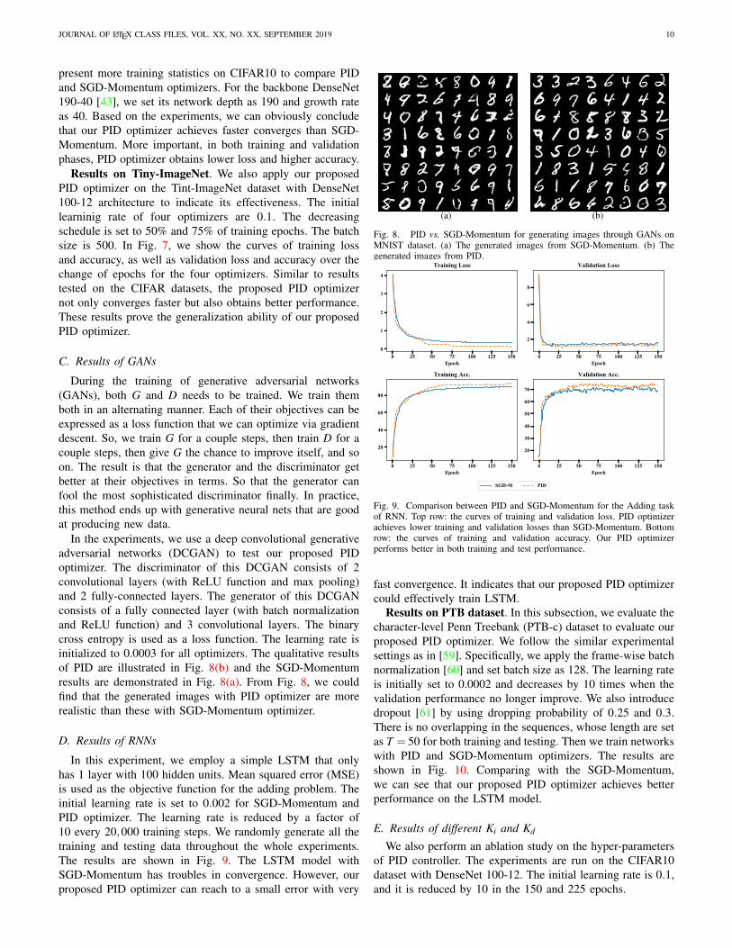
In the experiments, we use a deep convolutional generativeadversarial networks (DCGAN) to test our proposed PIDoptimizer. The discriminator of this DCGAN consists of 2convolutional layers (with ReLU function and max pooling)and 2 fully-connected layers. The generator of this DCGANconsists of a fully connected layer (with batch normalizationand ReLU function) and 3 convolutional layers. The binarycross entropy is used as a loss function. The learning rate isinitialized to 0.0003 for all optimizers. The qualitative resultsof PID are illustrated in Fig. 8(b) and the SGD-Momentumresults are demonstrated in Fig. 8(a). From Fig. 8, we couldfind that the generated images with PID optimizer are morerealistic than these with SGD-Momentum optimizer.

D. Results of RNNs

In this experiment, we employ a simple LSTM that onlyhas 1 layer with 100 hidden units. Mean squared error (MSE)is used as the objective function for the adding problem. Theinitial learning rate is set to 0.002 for SGD-Momentum andPID optimizer. The learning rate is reduced by a factor of10 every 20,000 training steps. We randomly generate all thetraining and testing data throughout the whole experiments.The results are shown in Fig. 9. The LSTM model withSGD-Momentum has troubles in convergence. However, ourproposed PID optimizer can reach to a small error with very

(a) (b)

Fig. 8. PID vs. SGD-Momentum for generating images through GANs onMNIST dataset. (a) The generated images from SGD-Momentum. (b) Thegenerated images from PID.

0 25 50 75 100 125 150Epoch

0

1

2

3

4

Training Loss

0 25 50 75 100 125 150Epoch

2

4

6

8

Validation Loss

0 25 50 75 100 125 150Epoch

20

40

60

80

Training Acc.

0 25 50 75 100 125 150Epoch

20

30

40

50

60

70

Validation Acc.

SGD-M PID

Fig. 9. Comparison between PID and SGD-Momentum for the Adding taskof RNN. Top row: the curves of training and validation loss. PID optimizerachieves lower training and validation losses than SGD-Momentum. Bottomrow: the curves of training and validation accuracy. Our PID optimizerperforms better in both training and test performance.

fast convergence. It indicates that our proposed PID optimizercould effectively train LSTM.

Results on PTB dataset. In this subsection, we evaluate thecharacter-level Penn Treebank (PTB-c) dataset to evaluate ourproposed PID optimizer. We follow the similar experimentalsettings as in [59]. Specifically, we apply the frame-wise batchnormalization [60] and set batch size as 128. The learning rateis initially set to 0.0002 and decreases by 10 times when thevalidation performance no longer improve. We also introducedropout [61] by using dropping probability of 0.25 and 0.3.There is no overlapping in the sequences, whose length are setas T = 50 for both training and testing. Then we train networkswith PID and SGD-Momentum optimizers. The results areshown in Fig. 10. Comparing with the SGD-Momentum,we can see that our proposed PID optimizer achieves betterperformance on the LSTM model.

E. Results of different Ki and Kd

We also perform an ablation study on the hyper-parametersof PID controller. The experiments are run on the CIFAR10dataset with DenseNet 100-12. The initial learning rate is 0.1,and it is reduced by 10 in the 150 and 225 epochs.

JOURNAL OF LATEX CLASS FILES, VOL. XX, NO. XX, SEPTEMBER 2019 11

0 5 10 15Epoch

0.2

0.4

0.6

0.8

Training Loss

0 5 10 15Epoch

0.10

0.15

0.20

0.25

0.30

0.35Validation Loss

0 5 10 15Epoch

85

90

95

Training Acc.

0 5 10 15 20Epoch

90

92

94

96

98

Validation Acc.

SGD-M PID

Fig. 10. Comparison between PID and SGD-Momentum to train LSTM onPTB dataset. Top row: the curves of training and validation loss. PID optimizerhelps to achieve smaller training and validation losses. Bottom row: the curvesof training and validation accuracy. PID optimizer helps to achieve higertraining and validation performance.

0 50 100 150 200 250 300Epoch

0.0

0.5

1.0

1.5

2.0

2.5

3.0

Training Loss

0 50 100 150 200 250 300Epoch

1

2

3

4Validation Loss

0 50 100 150 200 250 300Epoch

20

40

60

80

100Training Acc.

0 50 100 150 200 250 300Epoch

20

40

60

80

Validation Acc.

I=50 I=25 I=10 I=3 I=1 I=0.3

Fig. 11. Comparison among PID controllers with different Ki on theCIFAR10 dataset by using DenseNet 100-12. Kd is fixed to 10. Top row: thecurves of training and validation loss. Bottom row: the curves of training andvalidation accuracy. Within a certain range, larger Ki achieves better validationaccuracy.

The first group of experiments investigates the variation oftraining and verification statistics with Ki while Kd is fixed.Fig. 11 demonstrates six PID controllers whose Kd is 10. Inthe training, the performance of all controllers differ from eachother at an early stage, but eventually they can reach the samelevel. In validation, controller with Ki = 10 achieves lowestloss and highest validation accuracy. We also repeat this ex-periment with Kd = 10,25,50,and100 respectively, and resultsare highly similar to Fig. 11. One interesting phenomenon isthat the larger the Ki, the more affected by the decreasingschedule.

Then we change the research object to Kd . The settingsof the second group of experiments are kept the same asprevious experiments, but the Ki is fixed. Fig. 12 shows thattheir performance is highly consistent. It is also shown that the

0 50 100 150 200 250 300Epoch

0.0

0.5

1.0

1.5

2.0

2.5

3.0Training Loss

0 50 100 150 200 250 300Epoch

0.5

1.0

1.5

2.0

Validation Loss

0 50 100 150 200 250 300Epoch

20

40

60

80

100Training Acc.

0 50 100 150 200 250 300Epoch

40

60

80

Validation Acc.

D=100 D=50 D=25 D=10

Fig. 12. Comparison among PID controllers with different Kd on theCIFAR10 dataset by using DenseNet 100-12. Ki is fixed to 3. Top row: thecurves of training and validation loss. Bottom row: the curves of training andvalidation accuracy.

larger the Kd , the more unstable the validation performance.The reasons may be that large Kd leads to more change ofoptimization path.

As can be seen from these experiments, Ki is more importantthan Kd in this specific tasks (CIFAR10 with Densenet100-12).Ki not only affects the speed of convergence, but also affectsthe accuracy of verification.

VI. CONCLUSION AND FUTURE WORK

Motivated by the outstanding performance of proportional-integral-derivative (PID) controller in the field of automaticcontrol, we reveal the connections between PID controllerand stochastic optimizers and its variants. Then we propose anew PID optimizer used in deep neural network training. Theproposed PID optimizer reduces the overshoot phenomenonof SGD-momentum and accelerates the training process ofDNNs by combining the present, the past and the change in-formation of gradients to update parameters. Our experimentson both image recognition tasks with MNIST, CIFAR, andTiny-ImageNet datasets and LSTM tasks with PTB datasetvalidates that the proposed PID optimizer is 30% to 50% fasterthan SGD-Momentum, while obtaining lower error rate. Wewill continue to study the relationship among optimal hyper-parameters(Kp, Ki, and Kd) in specific task. We will conductmore in-depth researches for more general cases in the future.And we will investigate how to associate PID optimizer withan adaptive learning rate for DNNs/RNNs optimization infuture works.

ACKNOWLEDGMENT

This work is partially supported by the NSFC fund(61571259, 61831014, 61531014), in part by theShenzhen Science and Technology Project under Grant(GGFW2017040714161462, JCYJ20170307153051701).

JOURNAL OF LATEX CLASS FILES, VOL. XX, NO. XX, SEPTEMBER 2019 12

REFERENCES

[1] O. Russakovsky, J. Deng, H. Su, J. Krause, S. Satheesh, S. Ma,Z. Huang, A. Karpathy, A. Khosla, M. S. Bernstein, A. C. Berg, andF. fei Li, “Imagenet large scale visual recognition challenge,” IEEEInternational Journal of Computer Vision (IJCV), 2015.

[2] L. Bottou, “Large-scale machine learning with stochastic gradient de-scent,” in Proceedings of COMPSTAT’2010. Springer, 2010, pp. 177–186.

[3] J. Zhang, “Gradient descent based optimization algorithms for deeplearning models training,” arXiv preprint arXiv:1903.03614, 2019.

[4] E. L. Denton, W. Zaremba, J. Bruna, Y. LeCun, and R. Fergus,“Exploiting linear structure within convolutional networks for efficientevaluation,” in Advances in neural information processing systems, 2014,pp. 1269–1277.

[5] M. Jaderberg, A. Vedaldi, and A. Zisserman, “Speeding up convo-lutional neural networks with low rank expansions,” arXiv preprintarXiv:1405.3866, 2014.

[6] X. Zhang, J. Zou, K. He, and J. Sun, “Accelerating very deep convolu-tional networks for classification and detection,” IEEE transactions onpattern analysis and machine intelligence, vol. 38, no. 10, pp. 1943–1955, 2016.

[7] N. Vasilache, J. Johnson, M. Mathieu, S. Chintala, S. Piantino, andY. LeCun, “Fast convolutional nets with fbfft: A gpu performanceevaluation,” arXiv preprint arXiv:1412.7580, 2014.

[8] A. Romero, N. Ballas, S. E. Kahou, A. Chassang, C. Gatta, andY. Bengio, “Fitnets: Hints for thin deep nets,” International Conferenceon Learning Representations, 2015.

[9] D. J. Im, M. Tao, and K. Branson, “An empirical analysis of theoptimization of deep network loss surfaces,” in International Conferencefor Learning Representations (ICLR), 2017.

[10] I. Goodfellow, Y. Bengio, and A. Courville, Deep Learning. MIT Press,2016.

[11] L. Bottou, “Online learning in neural networks,” D. Saad, Ed.Cambridge University Press, 1998, ch. Online Learning and StochasticApproximations, pp. 9–42. [Online]. Available: http://dl.acm.org/citation.cfm?id=304710.304720

[12] I. Sutskever, J. Martens, G. Dahl, and G. Hinton, “On the importanceof initialization and momentum in deep learning,” in Internationalconference on machine learning, 2013.

[13] J. Duchi, E. Hazan, and Y. Singer, “Adaptive subgradient methodsfor online learning and stochastic optimization,” Journal of MachineLearning Research, vol. 12, no. Jul, pp. 2121–2159, 2011.

[14] G. Hinton, N. Srivastava, and K. Swersky, “Lecture 6a overview ofmini–batch gradient descent.”

[15] D. Kingma and J. Ba, “Adam: A method for stochastic optimization,” inInternational Conference for Learning Representations (ICLR), 2014.

[16] K. Ogata, Discrete-time control systems. Prentice Hall EnglewoodCliffs, NJ, 1995, vol. 2.

[17] L. Lessard, B. Recht, and A. Packard, “Analysis and design of opti-mization algorithms via integral quadratic constraints,” SIAM Journalon Optimization, vol. 26, no. 1, pp. 57–95, 2016.

[18] L. Wang, T. J. D. Barnes, and W. R. Cluett, “New frequency-domain de-sign method for pid controllers,” IEEE Control Theory and Applications,Jul 1995.

[19] K. Heong Ang, G. Chong, and Y. Li, “Pid control system analysis,design, and technology,” vol. 13, pp. 559 – 576, 08 2005.

[20] A. L. Salih, M. Moghavvemi, H. A. F. Mohamed, and K. S. Gaeid,“Modelling and pid controller design for a quadrotor unmanned airvehicle,” in IEEE International Conference on Automation, Quality andTesting, Robotics (AQTR), vol. 1, May 2010, pp. 1–5.

[21] P. Rocco, “Stability of pid control for industrial robot arms,” IEEEtransactions on robotics and automation, 1996.

[22] P. Zhao, J. Chen, Y. Song, X. Tao, T. Xu, and T. Mei, “Design ofa control system for an autonomous vehicle based on adaptive-pid,”International Journal of Advanced Robotic Systems, vol. 9, no. 2, p. 44,2012. [Online]. Available: https://doi.org/10.5772/51314

[23] P. S. de Laplace, Theorie analytique des probabilites. Courcier, 1820,vol. 7.

[24] W. An, H. Wang, Q. Sun, J. Xu, Q. Dai, and L. Zhang, “A pid controllerapproach for stochastic optimization of deep networks,” in The IEEEConference on Computer Vision and Pattern Recognition (CVPR), June2018.

[25] B. T. Polyak, “Some methods of speeding up the convergence of iter-ation methods,” USSR Computational Mathematics and MathematicalPhysics, vol. 4, no. 5, pp. 1–17, 1964.

[26] Y. Wei, W. Xia, M. Lin, J. Huang, B. Ni, J. Dong, Y. Zhao, andS. Yan, “Hcp: A flexible cnn framework for multi-label image classifica-tion,” IEEE Transactions on Pattern Analysis and Machine Intelligence,vol. 38, no. 9, pp. 1901–1907, Sept 2016.

[27] R. Girshick, J. Donahue, T. Darrell, and J. Malik, “Region-based convo-lutional networks for accurate object detection and segmentation,” IEEETransactions on Pattern Analysis and Machine Intelligence, vol. 38,no. 1, pp. 142–158, Jan 2016.

[28] S. Ren, K. He, R. Girshick, and J. Sun, “Faster r-cnn: Towards real-timeobject detection with region proposal networks,” IEEE Transactions onPattern Analysis and Machine Intelligence, vol. 39, no. 6, pp. 1137–1149, June 2017.

[29] W. Ouyang, X. Zeng, X. Wang, S. Qiu, P. Luo, Y. Tian, H. Li,S. Yang, Z. Wang, H. Li, K. Wang, J. Yan, C. C. Loy, and X. Tang,“Deepid-net: Object detection with deformable part based convolutionalneural networks,” IEEE Transactions on Pattern Analysis and MachineIntelligence, vol. 39, no. 7, pp. 1320–1334, July 2017.

[30] C. Farabet, C. Couprie, L. Najman, and Y. LeCun, “Learning hierarchicalfeatures for scene labeling,” IEEE transactions on pattern analysis andmachine intelligence, vol. 35, no. 8, pp. 1915–1929, 2013.

[31] I. Goodfellow, J. Pouget-Abadie, M. Mirza, B. Xu, D. Warde-Farley,S. Ozair, A. Courville, and Y. Bengio, “Generative adversarial nets,” inNIPS, 2014.

[32] S. Hochreiter and J. Schmidhuber, “Long short-term memory,” NeuralComputation, vol. 9, no. 8, pp. 1735–1780, 1997. [Online]. Available:https://doi.org/10.1162/neco.1997.9.8.1735

[33] M. Arjovsky, A. Shah, and Y. Bengio, “Unitary evolution recurrentneural networks,” in Proceedings of the 33nd International Conferenceon Machine Learning, ICML 2016, New York City, NY, USA,June 19-24, 2016, 2016, pp. 1120–1128. [Online]. Available:http://jmlr.org/proceedings/papers/v48/arjovsky16.html

[34] S. Han, H. Mao, and W. J. Dally, “Deep compression: Compressing deepneural networks with pruning, trained quantization and huffman coding,”in International Conference for Learning Representations (ICLR), 2015.

[35] Z. Liu, J. Li, Z. Shen, G. Huang, S. Yan, and C. Zhang, “Learning effi-cient convolutional networks through network slimming,” in Proceedingsof the IEEE International Conference on Computer Vision, 2017, pp.2736–2744.

[36] Y. He, P. Liu, Z. Wang, Z. Hu, and Y. Yang, “Filter pruning viageometric median for deep convolutional neural networks acceleration,”in Proceedings of the IEEE Conference on Computer Vision and PatternRecognition, 2019, pp. 4340–4349.

[37] X. Dai, H. Yin, and N. Jha, “Nest: A neural network synthesis tool basedon a grow-and-prune paradigm,” IEEE Transactions on Computers,2019.

[38] X. Du, Z. Li, and Y. Cao, “Cgap: Continuous growth and pruning forefficient deep learning,” arXiv preprint arXiv:1905.11533, 2019.

[39] I. Hubara, M. Courbariaux, D. Soudry, R. El-Yaniv, and Y. Bengio,“Quantized neural networks: Training neural networks with low pre-cision weights and activations,” The Journal of Machine LearningResearch, vol. 18, no. 1, pp. 6869–6898, 2017.

[40] R. Kidambi, P. Netrapalli, P. Jain, and S. M. Kakade, “On the insuffi-ciency of existing momentum schemes for stochastic optimization,” inInternational Conference for Learning Representations (ICLR), 2018.

[41] H. Li, A. Kadav, I. Durdanovic, H. Samet, and H. P. Graf, “Pruningfilters for efficient convnets,” arXiv preprint arXiv:1608.08710, 2016.

[42] K. He, X. Zhang, S. Ren, and J. Sun, “Deep residual learning forimage recognition,” in IEEE Conference on Computer Vision and PatternRecognition (CVPR), 2016.

[43] G. Huang, Z. Liu, L. van der Maaten, and K. Q. Weinberger, “Denselyconnected convolutional networks,” in IEEE Conference on ComputerVision and Pattern Recognition (CVPR), 2017.

[44] K. He, X. Zhang, S. Ren, and J. Sun, “Identity mappings in deep residualnetworks,” in IEEE European Conference on Computer Vision (ECCV),2016.

[45] S. Zagoruyko and N. Komodakis, “Wide residual networks,” in BMVC,2016.

[46] Y. Nesterov, “A method of solving a convex programming problem withconvergence rate o (1/k2),” in Soviet Mathematics Doklady, 1983.

[47] J. C. Maxwell, “On governors,” Proceedings of the Royal Society ofLondon, vol. 16, pp. 270–283, 1867.

[48] N. Minorsky, “Directional stability of automatically steered bodies,”Journal of ASNE, 1922.

[49] N. Qian, “On the momentum term in gradient descent learning algo-rithms,” Neural networks, vol. 12, no. 1, pp. 145–151, 1999.

[50] M. R. Spiegel, Advanced mathematics. McGraw-Hill, Incorporated,1991.

JOURNAL OF LATEX CLASS FILES, VOL. XX, NO. XX, SEPTEMBER 2019 13

[51] K. DE JONG, “An analysis of the behavior of a class of genetic adaptivesystems,” Doctoral Dissertation, University of Michigan, 1975.

[52] J. G. Ziegler and N. B. Nichols, “Optimum settings for automaticcontrollers,” trans. ASME, vol. 64, no. 11, 1942.

[53] G. E. Robert and H. Kaufman, Table of Laplace transforms. Saunders,1966.

[54] H. K. Khalil, Noninear Systems. Prentice-Hall, New Jersey, 1996.[55] Y. Le and X. Yang, “Tiny imagenet visual recognition challenge,” 2015.[56] Y. LeCun, L. Bottou, Y. Bengio, and P. Haffner, “Gradient-based learning

applied to document recognition,” Proceedings of the IEEE, vol. 86,no. 11, pp. 2278–2324, 1998.

[57] A. Krizhevsky, “Learning multiple layers of features from tiny images,”2009.

[58] S. Xie, R. Girshick, P. Dollar, Z. Tu, and K. He, “Aggregated residualtransformations for deep neural networks,” in IEEE Conference onComputer Vision and Pattern Recognition (CVPR), 2017.

[59] T. Cooijmans, N. Ballas, C. Laurent, and A. C. Courville, “Recurrentbatch normalization,” CoRR, vol. abs/1603.09025, 2016. [Online].Available: http://arxiv.org/abs/1603.09025

[60] C. Laurent, G. Pereyra, P. Brakel, Y. Zhang, and Y. Bengio, “Batchnormalized recurrent neural networks,” in 2016 IEEE InternationalConference on Acoustics, Speech and Signal Processing, ICASSP 2016,Shanghai, China, March 20-25, 2016, 2016, pp. 2657–2661. [Online].Available: https://doi.org/10.1109/ICASSP.2016.7472159

[61] Y. Gal and Z. Ghahramani, “A theoretically grounded application ofdropout in recurrent neural networks,” in Advances in Neural Informa-tion Processing Systems 29: Annual Conference on Neural InformationProcessing Systems 2016, December 5-10, 2016, Barcelona, Spain,2016, pp. 1019–1027.

Haoqian Wang (M’13) received the B.S. andM.E. degrees from Heilongjiang University, Harbin,China, in 1999 and 2002, respectively, and the Ph.D.degree from the Harbin Institute of Technology,Harbin, in 2005.He was a Post-Doctoral Fellow withTsinghua University, Beijing, China, from 2005 to2007. He has been a Faculty Member with theGraduate School at Shenzhen, Tsinghua University,Shenzhen, China, since 2008, where he has also beenan Associate Professor since 2011, and the directorof Shenzhen Institute of Future Media Technology.

His current research interests include generative adversarial networks, videocommunication and signal processing.

Yi Luo is received the B.E. degree in Xidian Uni-versity, Xi’an, China, in 2019. He is pursuing amaster degree in Tsinghua University. He is alsoworking as a research assistance in Graduate Schoolat Shenzhen, Tsinghua University, Shenzhen, China.His research interests include optimization in deeplearning.

Wangpeng An received the B.E. degree from Kun-ming University of Science and Technology in 2012.He is pursuing a master degree in Tsinghua Uni-versity, supervised by Professor Qionghai Dai. Hisresearch interests include face attribute recognition,generative adversarial networks and deep learningoptimization.

Qingyun Sun is current working toward the Ph.D.degree in Department of Mathematics, Stanford Uni-versity. He received B.S. from School of Mathemat-ical Sciences, Peking University, Beijing, China, in2014. His research interests include mathematicalfoundation for artificial intelligence, data science,machine learning, algorithmic game theory, multi-agent decision making, optimization, and high di-mensional statistics.

Jun Xu is an Assistant Professor in College of Com-puter Science, Nankai University, Tianjin, China.Before that, he worked as a Research Scientistin Inception Institute of Artificial Intelligence. Hereceived the B.Sc. degree in pure mathematics andthe M.Sc. degree in Information and Probability bothfrom the School of Mathematics Science, NankaiUniversity, Tianjin, China, in 2011 and 2014, re-spectively. He received the Ph.D. degree in 2018from the Department of Computing, The Hong KongPolytechnic University, supervised by Prof. David

Zhang and Prof. Lei Zhang.

Yongbing Zhang received the B.A. degree in En-glish and the M.S. and Ph.D degrees in computerscience from the Harbin Institute of Technology,Harbin, China, in 2004, 2006, and 2010, respec-tively. He joined Graduate School at Shenzhen, Ts-inghua University, Shenzhen, China in 2010, wherehe is currently an associate professor. He was thereceipt of the Best Student Paper Award at IEEEInternational Conference on Visual Communicationand Image Processing in 2015. His current researchinterests include signal processing, computational

imaging, and machine learning.

Yulun Zhang received B.E. degree from Schoolof Electronic Engineering, Xidian University, China,in 2013 and M.E. degree from Department of Au-tomation, Tsinghua University, China, in 2017. He iscurrently pursuing the Ph.D. degree with the Depart-ment of ECE, Northeastern University, USA. He wasthe receipt of the Best Student Paper Award at IEEEInternational Conference on Visual Communicationand Image Processing(VCIP) in 2015. He also wonthe Best Paper Award at IEEE International Confer-ence on Computer Vision (ICCV) RLQ Workshop

in 2019. His research interests include image restoration and deep learning.

Lei Zhang (M’04-SM’14-F’18) received his B.Sc.degree in 1995 from Shenyang Institute of Aeronau-tical Engineering, Shenyang, P.R. China, and M.Sc.and Ph.D degrees in Control Theory and Engineeringfrom Northwestern Polytechnical University, Xi’an,P.R. China, in 1998 and 2001, respectively. From2001 to 2002, he was a research associate in theDepartment of Computing, The Hong Kong Poly-technic University. From January 2003 to January2006 he worked as a Postdoctoral Fellow in theDepartment of Electrical and Computer Engineering,

McMaster University, Canada. In 2006, he joined the Department of Com-puting, The Hong Kong Polytechnic University, as an Assistant Professor.Since July 2017, he has been a Chair Professor in the same department. Hisresearch interests include Computer Vision, Image and Video Analysis, PatternRecognition, and Biometrics, etc. Prof. Zhang has published more than 200papers in those areas. As of 2019, his publications have been cited more than38,000 times in literature. Prof. Zhang is a Senior Associate Editor of IEEETrans. on Image Processing, and an Associate Editor of SIAM Journal ofImaging Sciences and Image and Vision Computing, etc. He is a ClarivateAnalytics Highly Cited Researcher from 2015 to 2018. More information canbe found in his homepage http://www4.comp.polyu.edu.hk/cslzhang/.