journal of la salient object detection via structured ...sjmaybank/salientobject.pdf · salient...

JOURNAL OF LATEX CLASS FILES, VOL. 13, NO. 9, SEPTEMBER 2014 1

Salient Object Detection viaStructured Matrix Decomposition

Houwen Peng, Bing Li, Haibin Ling, Weiming Hu, Weihua Xiong, and Stephen J. Maybank

Abstract—Low-rank recovery models have shown potential for salient object detection, where a matrix is decomposed into a low-rankmatrix representing image background and a sparse matrix identifying salient objects. Two deficiencies, however, still exist. First,previous work typically assumes the elements in the sparse matrix are mutually independent, ignoring the spatial and pattern relationsof image regions. Second, when the low-rank and sparse matrices are relatively coherent, e.g., when there are similarities between thesalient objects and background or when the background is complicated, it is difficult for previous models to disentangle them. Toaddress these problems, we propose a novel structured matrix decomposition model with two structural regularizations: (1) atree-structured sparsity-inducing regularization that captures the image structure and enforces patches from the same object to havesimilar saliency values, and (2) a Laplacian regularization that enlarges the gaps between salient objects and the background in featurespace. Furthermore, high-level priors are integrated to guide the matrix decomposition and boost the detection. We evaluate our modelfor salient object detection on five challenging datasets including single object, multiple objects and complex scene images, and showcompetitive results as compared with 24 state-of-the-art methods in terms of seven performance metrics.

Index Terms—Salient Object Detection, Matrix Decomposition, Low Rank, Structured Sparsity, Subspace Learning.

F

1 INTRODUCTION

V ISUAL saliency has been a fundamental research prob-lem in neuroscience, psychology and vision perception

for a long time. It refers to the identification of a subset ofvital visual information for further processing. As an im-portant branch of visual saliency, salient object detection isthe task of localizing and segmenting the most conspicuousforeground objects from a scene. It has received substantialattention over the last decade due to its wide range ofapplications in computer vision, such as object detection andrecognition [1]–[4], content-based image retrieval [5], [6] andcontext-aware image resizing [7]–[10].

Many saliency models have been proposed to computethe saliency map of a given image and detect the salient ob-jects. Depending on whether prior knowledge is used or not,current models fall into two categories: bottom-up and top-down. Bottom-up models [7], [11]–[17] are stimulus-drivenand essentially based upon local and/or global center-surround difference, using low-level features, such as color,texture and location. The main limitations of these methodsare that the detected salient regions may only contain partsof the target objects, or be easily mixed with background. Onthe other hand, top-down models [18]–[24] are task-drivenand usually exploit high-level human perceptual knowl-edge, such as context, semantics and background priors, to

• H. Peng is with the Institution of Automation, Chinese Academy ofSciences, Beijing 100190, China, and the Department of Computerand Information Sciences, Temple University, Philadelphia, PA. E-mail:[email protected].

• B. Li, W Xiong and W. Hu are with the Institution of Automation,Chinese Academy of Sciences, Beijing 100190, China. E-mail: bli,[email protected], [email protected].

• H. Ling is with the Department of Computer and Information Sciences,Temple University, Philadelphia, PA. E-mail: [email protected].

• S. Maybank is with the Department of Computer Science and InformationSystems, Birkbeck College, London WC1E 7HX, United Kingdom. E-mail:[email protected].

Manuscript received XXX XX, 2015.

guide the subsequent saliency computation. However, thehigh diversity of object types limits the generalization andscalability of these models.

A recent trend is to combine bottom-up cues with top-down priors to facilitate detection. A representative seriesof papers [25]–[28] are based on the low-rank matrix recovery(LR) theory [29]. For instance, Shen and Wu [26] proposea unified LR model (ULR) with feature transformation tocombine traditional low-level features with high-level priorknowledge. Zou et al. [28] introduce the segmentation priorsderived from image background and boundary cues toassist the low-rank matrix recovery (denoted as SLR). Langet al. [27] present a low-rank representation (LRR) [30] basedmulti-task learning method, in which top-down priors areweighted and combined with multiple features to estimatesaliency collaboratively. Generally, these LR-based saliencydetection methods assume that an image can be representedas a combination of a highly redundant information part(e.g., visually consistent background regions) and a sparsesalient part (e.g., distinctive foreground object regions). Theredundant information part usually lies in a low dimension-al feature subspace, which can be approximated by a low-rank feature matrix. In contrast, the salient part deviatingfrom the low-rank subspace can be viewed as noise orerrors, which are represented by a sparse sensory matrix.Therefore, given the feature matrix F of an input image, itcan be decomposed as a low-rank matrix L correspondingto the non-salient background and a sparse matrix S cor-responding to the salient foreground objects. Salient objectdetection can then be formulated as a low-rank matrixrecovery problem [29]:

minL,S‖L‖∗+λ‖S‖1 s.t. F = L + S , (1)

where the nuclear norm ‖·‖∗ (sum of the singular valuesof a matrix) is a convex relaxation of the matrix rank


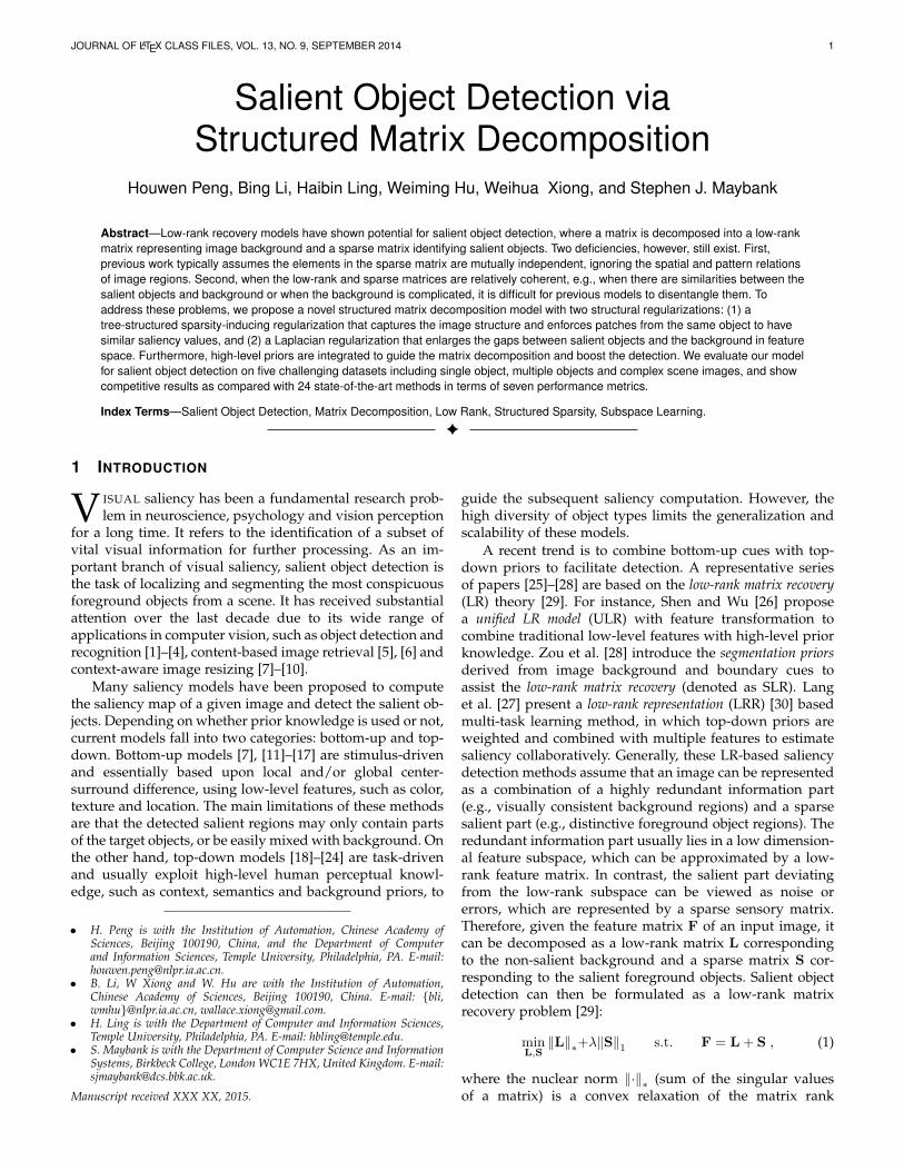
Image LRR [27] ULR [26] SLR [28] SMD(ours) GTFig. 1. Typical challenging examples for LR-based salient object de-tection algorithms. The resulting saliency maps of previous solutions(LRR [27], ULR [26] and SLR [28]) are scattered and incomplete, whileour algorithm (SMD) overcomes these difficulties and performs close tothe ground truth (GT).

function, ‖·‖1 is the `1-norm which promotes sparsity, andthe parameter λ > 0 controls the tradeoff between the twoitems.

Though previous LR-based salient object detection algo-rithms ( [26]–[28]) have produced promising results, therestill exist several problems:• Previous studies do not take into account the inter-

correlation between elements in S, and thus ignorespatial relations, such as spatial contiguity and patternconsistency, between pixels and patches. Algorithms de-signed this way may suffer from two limitations: (1) theforeground pixels or patches in the generated saliencymap tend to be scattered, as shown in Fig. 1 (LRR andULR); and (2) the saliency values may be inconsistentwithin the same object, causing incompleteness of thedetected object, as shown in Fig. 1 (LRR, ULR and SLR).

• According to the LR theory (a.k.a robust PCA) [29], thedecomposition performance of an observation matrixdegrades when there is high coherence between the un-derlying low-rank and sparse matrices. Therefore, whenthe background is cluttered or has similar appearancewith the salient objects, it is difficult for previous LR-based methods to separate them, as shown in the lasttwo rows of Fig. 1.To address these issues, we propose a novel structured

matrix decomposition (SMD) model that treats the (salient)foreground/background separation as a problem of low-rank and structured-sparse matrix decomposition. We en-hance the traditional LR model in Eq. (1) with two importantcomponents. First, we introduce a tree-structured sparsity-inducing norm to constrain S, so that the spatial connectivityand feature similarity of image patches are taken into ac-count in matrix decomposition. This constraint is essentiallya hierarchical group sparsity norm over a tree structure,in which an `∞-norm is employed to enforce within-objectpatches to share consistent saliency values. Second, weintegrate a Laplacian regularization to reduce the coherencebetween the low-rank and structured-sparse matrices. Theregularizer takes into account the geometrical structure ofthe image, encourages local similar patches to share similarrepresentation, and eventually separates the foregroundobjects from the background as much as possible. These

properties enable the proposed SMD model to detect salientobjects in jumbled scenes, even when the salient objects havea similar appearance to the background. In addition, SMDenhances object completeness which is sometime hard toachieve by previous solutions.

The main contributions of this work are summarized asfollows:• We develop a novel structured matrix decomposition

model, i.e., SMD, for salient object detection. Comparedto the classical LR model used in [26]–[28], SMD not onlycaptures the underlying structure of data, but also betterhandles the challenges arising from coherence of thelow-rank and sparse matrices. To the best of our knowl-edge, this is the first work that explicitly pursues thehierarchical structure of data via structured sparsity inmatrix decomposition. Based on the alternating directionmethod (ADM) [31], we derive an effective optimizationalgorithm to solve the proposed SMD model.

• We present an SMD-based salient object detection frame-work and evaluate the SMD method on five popularbenchmarks involving various scenarios such as singleobject, multiple objects and complex scenes. Also, wecompare our method with 24 state-of-the-art method-s using six performance metrics, including the tradi-tional measures, e.g., precision-recall curve and meanabsolute error, and the recently proposed weighted F -measure [32]. In the experiments, our SMD-based algo-rithm achieves competitive results in comparison withother leading methods.The remainder of this paper is organized as follows. Sec.

2 reviews existing saliency detection models, especially theLR-based methods. Sec. 3 describes the proposed SMD mod-el and derives the ADM-based solution to the model. Sec.4 presents the SMD-based salient object detection methodand extends it to integrate high-level priors. Sec. 5 showsthe experimental results, including a thorough comparisonwith recently proposed salient object detection algorithmsand detailed analysis of the components in our algorithm.Finally, Sec. 6 concludes the paper.

2 RELATED WORK

Recent years have witnessed significant advances in saliencydetection that includes two major subfields: eye fixationprediction and salient object detection. Recent surveys oneye fixation prediction can be found in [33]–[35], and salientobject detection is surveyed in [36], [37]. In this section,we mainly discuss the algorithms belonging to the secondsubfield, to which our work belongs. But before that, webriefly review some classical early studies that have pavedthe way to both subfields.

The foundation of most saliency detection algorithm-s can be traced back to the theories of center-surrounddifference [38] and multiple feature integration [39]. Themost influential model based on the theories is proposedby Itti et al. [11], who derive saliency from the difference ofGaussians on multiple feature maps. Another early work isby Harel et al. [40] who define a graph on image and adoptrandom walks to compute saliency. Some learning-basedmethods [41], [42] are also proposed to predict saliency bycombining multiple feature maps. Latter, researchers refine


the theories by taking account of local [43], [44], regional[45], and global [46] contrast cues, or by searching forsaliency cues in the frequency domain [14], [47].

One of the earliest works on salient object detection is [48],which formulates saliency detection as a binary segmen-tation problem. Recent studies can be broadly categorizedas either bottom-up or top-down. Bottom-up models arebio-inspired and only use low-level image features. Thefrequency tuning method [49] detects saliency by computingcolor deviation from the mean image color at the pixel level.Later, an improved solution [7] is proposed to highlightsalient objects with respect to their contexts in terms oflow-level feature distinction and global spatial relations.The global contrast method [12] identifies salient regions byestimating dissimilarities between Lab color histograms overall image regions. Saliency filters [50] improve the globalcontrast method [12] by combining color uniqueness andspatial distribution of image regions. Some other bottom-up techniques such as multi-scale modeling [51] and high-dimensional color transformation [17] have been exploredfor salient object detection. The effectiveness of other com-plementary cues such as texture [20], depth [52], [53] orsurroundedness [54] have also been considered recently.

By contrast, top-down models usually estimate saliencyvia task-specific learning algorithms or high-level priors.The method in [48] identifies salient objects using a condi-tional random field (CRF) on a multi-scale contrast histogramand spatial distribution features. The latent variable modelin [55] estimates saliency by jointly learning a CRF anda specific dictionary. Instead of direct training on imagefeatures, saliency aggregation [56] trains a CRF on salien-cy maps produced by other methods. The random forestmodel [57] predicts image saliency by training a regressoron discriminative regional features. Most recently, multiplekernel learning [58] and convolutional neural network [59]techniques have been introduced to learn more robust dis-crimination between salient and non-salient regions.

High-level priors have also been used in top-down mod-els and proved to be effective. For example, a Gaussian fall-off function is frequently recruited to emphasize the centerregions (i.e., center prior), either directly combined with othercues [19], [21], [60], or used as a spatial feature in learn-ing [48], [57]. The prior belief that image boundary regionsare more likely to belong to the background (i.e., backgroundprior) is also commonly integrated for saliency computation.A representative work is the geodesic saliency [24], whichdefines boundary regions as terminal nodes when estimat-ing saliency on an image graph. Alternatively, in [61], [62],boundary regions are used as pseudo-background queriesand dictionary templates to facilitate detection. Later, a morerobust boundary connectivity prior is introduced in [63].Besides, the objectness prior, which estimates the likelihoodof a region being a complete object [2], has been employedin some other saliency models [18], [64], [65].

Our study is related to recent methods that considerthe sparsity prior in salient object detection. The method in[25] adopts an over-complete dictionary to encode imagepatches and then feed the coding vector to the LR modelto recover salient objects. Later, a supervised method [26] isproposed to leverage feature transformation with the high-level center, color and semantic priors to meet the low-

rank and sparse properties. To better fit the LR model, thesegmentation prior derived from the connectivity betweenregions and image borders is exploited to guide matrix re-covery [28]. As an extension of the LR model, low-rank repre-sentation (LRR) [27] introduces a self-representation schemethat reconstructs background regions from the image fea-tures themselves rather than by a dictionary. Multi-featurecollaborative enhancement and top-down priors obtainedfrom [66] are incorporated into the multi-task extension.

Difference to related LR-based methods. As an LR-basedmethod, our SMD differs from the previous ones [25]–[28]in several aspects. (1) SMD pursues the low matrix rankin a purely unsupervised way, while [25] and [26] respec-tively resort to supervised sparse representation and featuretransformation. The learnt representation or transformationin [25] and [26] is biased toward the training datasets, andtherefore suffers from limited adaptability. (2) Our methodexplicitly encodes information about image structure, i.e.,spatial relations and feature similarities of image patches,which are ignored in [25]–[28]. (3) Our method integrateshigh-level priors into the structured image representation(index tree), while other methods [26], [28] combine suchpriors by re-weighting the feature.

Discussion with Manifold Ranking (MR) methods. The useof the Laplacian regularization in our method is inspiredby, but different from that in the MR algorithm [61]. (1)Our method uses the Laplacian regularization to smooth thefeature representation, and to enlarge the difference betweenforeground objects and background in feature space. By con-trast, MR exploits the regularization to enforce continuoussaliency values over neighboring patches. (2) MR is builtupon the semi-supervised ranking model [67], and definessaliency of an patch as its relevance to the given queryingseeds. By contrast, our method uses the low-rank matrixdecomposition framework and is purely unsupervised.

Difference with preliminary work. Some preliminary ideasin this paper appeared in the conference version [68]. Com-pared with [68], the proposed SMD model in this paperis more general, and subsumes the version in [68] as aspecial case. The new SMD model not only inherits themajor advantages of the preliminary model, i.e., it producesa decomposition of an observation matrix into structuredparts with respect to image structure, but it is also armedwith the new capability to enlarge the separation betweensalient objects and background in the feature space. Theexperimental results (Sec. 5) show clearly that the newmodel is more robust and the resulting saliency maps (Fig.8) are more visually favorable.

3 STRUCTURED MATRIX DECOMPOSITION MODEL

3.1 Proposed Model

3.1.1 Basic formulationGiven an input image I , it is first partitioned into N non-overlapping patches P = P1, P2, · · · , PN, e.g., superpix-els. For each patch Pi, a D-dimension feature vector isextracted and denoted as fi ∈ RD. The ensemble of featurevectors forms a matrix representation of I , denoted asF = [f1, f2, . . . , fN ] ∈ RD×N . The problem of salient objectdetection is to design an effective model to decompose thefeature matrix F into a redundant information part L (i.e.,


2 4 6 8 10 12 14 16 18 20 22 240

0.05

0.1

0.15

0.2

0.25

0.3

0.35

0.4

Rank r of Feature Matrix

ProbabilityofOccurence

MSRA10KDUT-OMRONiCoSegSODECSSD

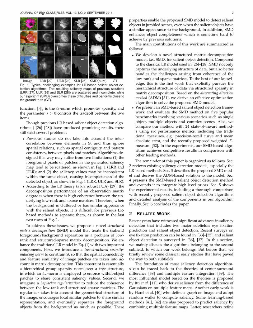
Fig. 2. Rank statistics of feature matrices extracted from image back-ground over five datasets: MSRA10K [48], [69], DUT-OMRON [61], SOD[70], iCoSeg [71] and ECSSD [21].

non-salient background) and a structured distinctive part S(i.e., salient foreground).

To address the issues discussed in Sec. 1, we proposea novel structured matrix decomposition (SMD) model as fol-lows:

minL,S

Ψ(L) + αΩ(S) + βΘ(L,S) s.t. F = L + S , (2)

where Ψ(·) is a low-rank constraint to allow identification ofthe intrinsic feature subspace of the redundant backgroundpatches, Ω(·) is a structured sparsity regularization to cap-ture the spatial and feature relations of patches in S, Θ(·, ·)is an interactive regularization term to enlarge the distancebetween the subspaces drawn from L and S, and α, β arepositive tradeoff parameters.

3.1.2 Low-rank regularization for image backgroundHaving observed that image patches from the backgroundare often similar and approximately lie in a low-dimensionalsubspace, we apply low-rank regularization on the back-ground feature matrix L to pursue its intrinsic structure.Since directly minimizing a matrix’s rank with affine con-straints is an NP-hard problem [30], we instead adopt thenuclear norm as a convex relaxation, i.e.,

Ψ(L) = rank(L) = ‖L‖∗ + ε , (3)

where ε denotes the relaxation error.To verify the rationality of the low-rank constraint, we

evaluate the rank of feature matrices extracted from imagebackground on five salient object datasets (Fig. 2). Specifical-ly, we first divide each image into a regular grid of patchesof size 10×10 pixels, excluding those “foreground” patches,which have over 10% pixels from the annotated salientobjects. Then, each patch is represented by a feature vectorencoding color, edge and texture information (as describedin Sec. 4.1). Features from the same image are juxtaposedinto a matrix to represent the image background. Finally,we estimate the rank of the feature matrix, denoted by r,according to [72], [73]:

r = arg minr

(RMSRE(r − 1)− RMSRE(r)

)≤ ε , (4)

where RMSRE(r) is the root mean square reconstruction errorbetween the original matrix and its rank-r approximationestimated by the singular value decomposition (SVD), and εis a threshold with value 0.01. Fig. 2 shows the statisticsof such estimated ranks of background feature matrices ofthe images in the five datasets. It shows that about 90%of these matrices can be approximated by a matrix with

1

2 3 65

4 87

1

2 3 5

4 87

81

1G

2

1G

2

3G

3

1G3

3G

3

4G

3

5G

3 65

4 7

6

1

2

3

2G

(A) (B)

2

2G

1

1G

2

1G2

2G

3

4G

2

3G

3

3G3

2G3

1G

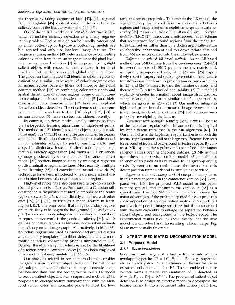
Fig. 3. The construction of an index tree from an image. (A): Thehierarchical segmentation of an input image. The digits are the indexesof patches. (B): An index tree constructed over the indices of imagepatches 1, 2, . . . , 8. Depth 1 (Root): G1

1 = 1, 2, 3, 4, 5, 6, 7, 8. Depth2: G2

1 = 1, 2, 3, 4, G22 = 5, 6, G2

3 = 7, 8. Depth 3: G31 = 1, 2,

G32 = 3, 4, G3

3 = 5, G34 = 6.

rank no greater than 10. This confirms our intuition thatthe image background usually lies in a low-dimensionalsubspace. Therefore, it encourages us to exploit a low-rank regularization to eliminate redundant information andpursue the intrinsic low-dimensional structure.

3.1.3 Structured-sparsity regularization for salient objects

In Eq. (1), the `1-norm regularization treats the columns inS independently and thus ignores spatial structure informa-tion, which can otherwise be used to improve salient objectdetection (see Fig. 1). In the following, we introduce a noveltree-structured sparsity-inducing norm to model the spatialcontiguity and feature similarity among image patches so asto produce more precise and structurally consistent results.

Before detailing the structured regularization, we firstgive the definition of an index tree [74]. An index tree is ahierarchial structure, such that each node contains a set ofindices (e.g., corresponding to the superpixels in our task)and the set is the union of the indices of its children. Morespecifically, for an index tree T with depth d over indices1, 2, . . . , N, let Gij be the j-th node at the i-th level. Inparticular, for the root node, we have G1

1 = 1, 2, . . . , N.The nodes also satisfy two conditions: (1) there is no overlapbetween the indices of nodes from the same level, i.e., Gij ∩Gik = ∅, ∀2 ≤ i ≤ d and 1 ≤ j < k ≤ ni. Here, ni denotesthe total number of nodes at the i-th level. (2) Let Gi−1j0 bethe parent node of a non-root node Gij , then Gij ⊆ G

i−1j0 and⋃

j Gij = Gi−1j0 . Fig. 3 shows an example tree with N = 8

indexes, drawn from hierarchical segmentation of an image.We use an index tree T to encode the spatial relation of

image patches P . Details of index tree construction are post-poned to Sec. 4.1. We encode the structurally meaningfultree constraint into a sparsity norm to regularize the matrixdecomposition. In this way, we get a general tree-structuredsparsity regularization as

Ω(S) =d∑i=1

ni∑j=1

vij‖SGij‖p , (5)

where vij ≥ 0 is the weight for the node Gij , SGij∈ RD×|G

ij|

(|·| denotes set cardinality) is the sub-matrix of S corre-sponding to the node Gij , and ‖·‖p is the `p-norm1, 1 ≤p ≤ ∞. In essence, Ω(·) is a weighted group sparsity normdefined over a tree structure. It induces the patches within

1. For a matrix A = (aij) ∈ Rm×n, ‖A‖p = (m∑i=1

n∑j=1

|ai,j |p)1/p.


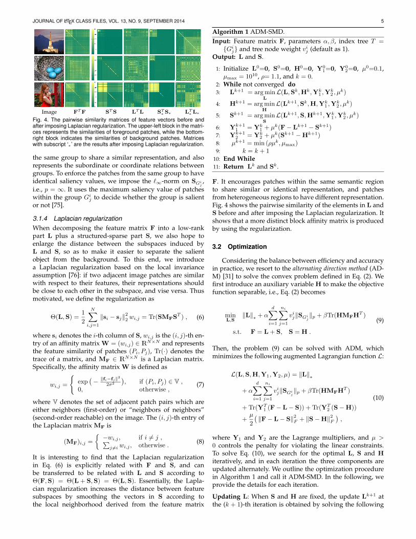
Image FTF STS LTL ST∗ S∗ LT

∗ L∗

Fig. 4. The pairwise similarity matrices of feature vectors before andafter imposing Laplacian regularization. The upper-left block in the matri-ces represents the similarities of foreground patches, while the bottom-right block indicates the similarities of background patches. Matriceswith subscript ‘∗’ are the results after imposing Laplacian regularization.

the same group to share a similar representation, and alsorepresents the subordinate or coordinate relations betweengroups. To enforce the patches from the same group to haveidentical saliency values, we impose the `∞-norm on SGi

j,

i.e., p = ∞. It uses the maximum saliency value of patcheswithin the group Gij to decide whether the group is salientor not [75].

3.1.4 Laplacian regularizationWhen decomposing the feature matrix F into a low-rankpart L plus a structured-sparse part S, we also hope toenlarge the distance between the subspaces induced byL and S, so as to make it easier to separate the salientobject from the background. To this end, we introducea Laplacian regularization based on the local invarianceassumption [76]: if two adjacent image patches are similarwith respect to their features, their representations shouldbe close to each other in the subspace, and vise versa. Thusmotivated, we define the regularization as

Θ(L,S) =1

2

N∑i,j=1

‖si − sj‖22 wi,j = Tr(SMFST ) , (6)

where si denotes the i-th column of S, wi,j is the (i, j)-th en-try of an affinity matrix W = (wi,j) ∈ RN×N and representsthe feature similarity of patches (Pi, Pj), Tr(·) denotes thetrace of a matrix, and MF ∈ RN×N is a Laplacian matrix.Specifically, the affinity matrix W is defined as

wi,j =

exp

(− ‖fi−fj‖

2

2σ2

), if (Pi, Pj) ∈ V ,

0, otherwise ,(7)

where V denotes the set of adjacent patch pairs which areeither neighbors (first-order) or “neighbors of neighbors”(second-order reachable) on the image. The (i, j)-th entry ofthe Laplacian matrix MF is

(MF)i,j =

−wi,j , if i 6= j ,∑j 6=i wi,j , otherwise .

(8)

It is interesting to find that the Laplacian regularizationin Eq. (6) is explicitly related with F and S, and canbe transferred to be related with L and S according toΘ(F,S) = Θ(L + S,S) = Θ(L,S). Essentially, the Lapla-cian regularization increases the distance between featuresubspaces by smoothing the vectors in S according tothe local neighborhood derived from the feature matrix

Algorithm 1 ADM-SMD.Input: Feature matrix F, parameters α, β, index tree T =Gij and tree node weight vij (default as 1).

Output: L and S.

1: Initialize L0=0, S0=0, H0=0, Y01=0, Y0

2=0, µ0=0.1,µmax = 1010, ρ= 1.1, and k = 0.

2: While not converged do3: Lk+1 = arg min

LL(L,Sk,Hk,Yk

1 ,Yk2 , µ

k)

4: Hk+1 = arg minH

L(Lk+1,Sk,H,Yk1 ,Y

k2 , µ

k)

5: Sk+1 = arg minS

L(Lk+1,S,Hk+1,Yk1 ,Y

k2 , µ

k)

6: Yk+11 = Yk

1 + µk(F− Lk+1 − Sk+1)7: Yk+1

2 = Yk2 + µk(Sk+1 −Hk+1)

8: µk+1 = min (ρµk, µmax)9: k = k + 1

10: End While11: Return Lk and Sk.

F. It encourages patches within the same semantic regionto share similar or identical representation, and patchesfrom heterogeneous regions to have different representation.Fig. 4 shows the pairwise similarity of the elements in L andS before and after imposing the Laplacian regularization. Itshows that a more distinct block affinity matrix is producedby using the regularization.

3.2 Optimization

Considering the balance between efficiency and accuracyin practice, we resort to the alternating direction method (AD-M) [31] to solve the convex problem defined in Eq. (2). Wefirst introduce an auxiliary variable H to make the objectivefunction separable, i.e., Eq. (2) becomes

minL,S

‖L‖∗ + αd∑i=1

ni∑j=1

vij‖SGij‖p + βTr(HMFHT )

s.t. F = L + S, S = H .

(9)

Then, the problem (9) can be solved with ADM, whichminimizes the following augmented Lagrangian function L:

L(L,S,H,Y1,Y2, µ) = ‖L‖∗

+ αd∑i=1

ni∑j=1

vij‖SGij‖p + βTr(HMFHT )

+ Tr(YT1 (F− L− S)) + Tr(YT

2 (S−H))

+µ

2

(‖F− L− S‖2F + ‖S−H‖2F

),

(10)

where Y1 and Y2 are the Lagrange multipliers, and µ >0 controls the penalty for violating the linear constraints.To solve Eq. (10), we search for the optimal L, S and Hiteratively, and in each iteration the three components areupdated alternately. We outline the optimization procedurein Algorithm 1 and call it ADM-SMD. In the following, weprovide the details for each iteration.

Updating L: When S and H are fixed, the update Lk+1 atthe (k + 1)-th iteration is obtained by solving the following


problem:

Lk+1 = arg minL

L(L,Sk,Hk,Yk1 ,Y

k2 , µ

k)

= arg minL

‖L‖∗ + Tr((Yk1 )T (F− L− Sk))

+µk

2‖F− L− Sk‖2F

= arg minL

τ‖L‖∗ +1

2‖L−XL‖2F ,

(11)

where τ = 1/µk and XL = F− Sk + Yk1/µ

k. The solution toEq. (11) can be derived as

Lk+1=UTτ [Σ]VT ,where (U,Σ,VT ) =SVD(XL) . (12)

Note that Σ is the singular value matrix of XL. The operatorTτ [· ] is the singular value thresholding (SVT) [77] defined byelement-wise τ thresholding of Σ. Specifically, let σi be thei-th diagonal element of Σ, then Tτ [Σ] is a diagonal matrixdefined as

Tτ [Σ] = diag((σi − τ)+), (13)

where a+ is the positive part of a, namely, a+ = max(0, a).

Updating H: When L and S are fixed, to update Hk+1, wederive from Eq. (10) the following problem:

Hk+1 = arg minH

L(Lk+1,Sk,H,Yk1 ,Y

k2 , µ

k)

= arg minH

βTr(HMFHT )+Tr((Yk2 )T (Sk−H))

+µk

2‖Sk−H‖2F .

(14)

Taking derivative of the objective function in Eq. (14) (thedetailed derivation is presented in Appendix A), we have

Hk+1 = (µkSk + Yk2 )(2βMF + µkI)−1 . (15)

Updating S: To update Sk+1 with fixed L and H, we get thefollowing tree-structured sparsity optimization problem:

Sk+1= arg minS

L(Lk+1,S,Hk+1,Yk1 ,Y

k2 , µ

k)

= arg minS

αd∑i=1

ni∑j=1

vij‖SGij‖p

+Tr((Yk1 )T(F−Lk+1−S))+Tr((Yk

2 )T(S−Hk+1))

+µk

2(‖F−Lk+1−S‖2F + ‖S−Hk+1‖2F )

= arg minS

λd∑i=1

ni∑j=1

vij‖SGij‖p +

1

2‖S−XS‖2F ,

(16)

where λ = α/(2µk) and XS = (F−Lk+1+Hk+1 + (Yk1 −

Yk2 )/µk)/2. The above problem can be solved by the hierar-

chical proximal operator [78], which computes a particularsequence of residuals obtained by projecting a matrix ontothe unit ball of dual `p-norm. The detailed procedure whenusing `∞-norm is presented in Algorithm 2.

4 SMD-BASED SALIENT OBJECT DETECTION

In this section, we describe our salient object detection algo-rithm that uses the proposed SMD model. Our algorithmincludes two major parts: the first one focuses on low-level features, while the second one incorporates high-levelprior knowledge. Fig. 5 shows the framework of SMD-basedsalient object detection.

Algorithm 2 Solving the tree-structured sparsity.

Input: The index tree T with nodes Gij (i = 1, 2, ..., d; j =1, 2, ..., ni), weight vij ≥ 0 (default as 1), the matrix XS,parameters α, and set λ = α/(2µk).

1: Set S = XS

2: For i = d to 1 do3: For j = 1 to ni do

4: Sk+1Gi

j=

∥∥S

Gij

∥∥1−λvij∥∥S

Gij

∥∥1

SGij, if

∥∥SGij

∥∥1> λvij

0, otherwise5: End For6: End For7: Return Sk+1

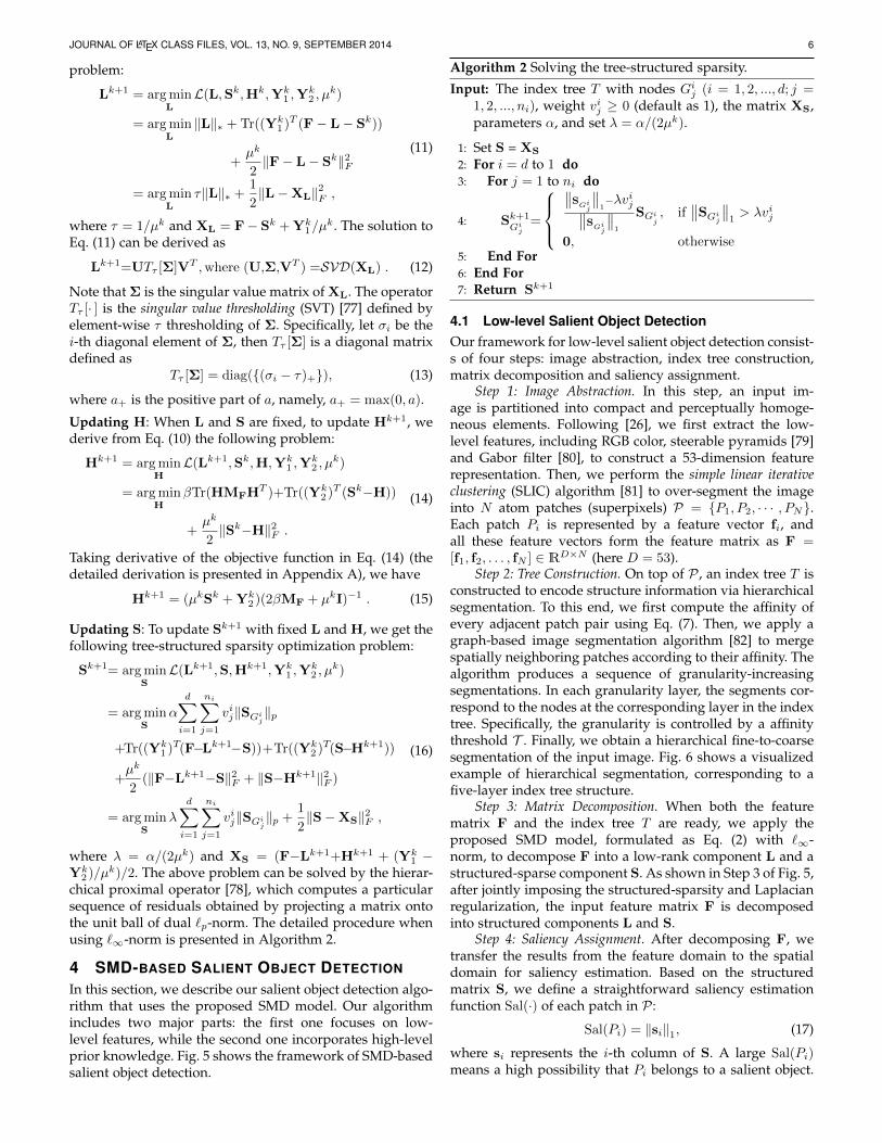
4.1 Low-level Salient Object DetectionOur framework for low-level salient object detection consist-s of four steps: image abstraction, index tree construction,matrix decomposition and saliency assignment.

Step 1: Image Abstraction. In this step, an input im-age is partitioned into compact and perceptually homoge-neous elements. Following [26], we first extract the low-level features, including RGB color, steerable pyramids [79]and Gabor filter [80], to construct a 53-dimension featurerepresentation. Then, we perform the simple linear iterativeclustering (SLIC) algorithm [81] to over-segment the imageinto N atom patches (superpixels) P = P1, P2, · · · , PN.Each patch Pi is represented by a feature vector fi, andall these feature vectors form the feature matrix as F =[f1, f2, . . . , fN ] ∈ RD×N (here D = 53).

Step 2: Tree Construction. On top of P , an index tree T isconstructed to encode structure information via hierarchicalsegmentation. To this end, we first compute the affinity ofevery adjacent patch pair using Eq. (7). Then, we apply agraph-based image segmentation algorithm [82] to mergespatially neighboring patches according to their affinity. Thealgorithm produces a sequence of granularity-increasingsegmentations. In each granularity layer, the segments cor-respond to the nodes at the corresponding layer in the indextree. Specifically, the granularity is controlled by a affinitythreshold T . Finally, we obtain a hierarchical fine-to-coarsesegmentation of the input image. Fig. 6 shows a visualizedexample of hierarchical segmentation, corresponding to afive-layer index tree structure.

Step 3: Matrix Decomposition. When both the featurematrix F and the index tree T are ready, we apply theproposed SMD model, formulated as Eq. (2) with `∞-norm, to decompose F into a low-rank component L and astructured-sparse component S. As shown in Step 3 of Fig. 5,after jointly imposing the structured-sparsity and Laplacianregularization, the input feature matrix F is decomposedinto structured components L and S.

Step 4: Saliency Assignment. After decomposing F, wetransfer the results from the feature domain to the spatialdomain for saliency estimation. Based on the structuredmatrix S, we define a straightforward saliency estimationfunction Sal(·) of each patch in P :

Sal(Pi) = ‖si‖1, (17)

where si represents the i-th column of S. A large Sal(Pi)means a high possibility that Pi belongs to a salient object.


Original Image

Saliency MapA Structured Index Tree

Over-segmentation

if

Low Rank Part (L) Structured Sparse Part (S)

Gi

j

Feature Extraction Feature Matrix (F)

High-level Prior

Map

Location

Prior

Color

Prior

Background

Prior

1

1G

2

1G 2

jG

1

dG

2

2

nG

1d

d

nG -d

d

nG'j

dG2

dG

iP

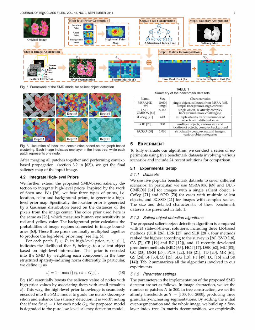
Fig. 5. Framework of the SMD model for salient object detection.

Depth5 Depth4

Depth3 Depth2 Depth1

Fig. 6. Illustration of index tree construction based on the graph-basedclustering. Each image indicates one layer in the index tree, while eachpatch represents one node.

After merging all patches together and performing context-based propagation (section 3.2 in [62]), we get the finalsaliency map of the input image.

4.2 Integrate High-level PriorsWe further extend the proposed SMD-based saliency de-tection to integrate high-level priors. Inspired by the workof Shen and Wu [26], we fuse three types of priors, i.e.location, color and background priors, to generate a high-level prior map. Specifically, the location prior is generatedby a Gaussian distribution based on the distances of thepixels from the image center. The color prior used here isthe same as [26], which measures human eye sensitivity tored and yellow color. The background prior calculates theprobabilities of image regions connected to image bound-aries [63]. These three priors are finally multiplied togetherto produce the high-level prior map (see Fig. 5).

For each patch Pi ∈ P , its high-level prior, πi ∈ [0, 1],indicates the likelihood that Pi belongs to a salient objectbased on high-level information. This prior is encodedinto the SMD by weighting each component in the tree-structured sparsity-inducing norm differently. In particular,we define vij as

vij = 1−max(πk : k ∈ Gij

). (18)

Eq. (18) essentially boosts the saliency value of nodes withhigh prior values by associating them with small penaltiesvij . This way, the high-level prior knowledge is seamlesslyencoded into the SMD model to guide the matrix decompo-sition and enhance the saliency detection. It is worth notingthat if we fix vij = 1 for each node Gij , the proposed modelis degraded to the pure low-level saliency detection model.

TABLE 1Summary of the benchmark datasets.

Name Size CharacteristicsMSRA10K

[69]10,000(imgs)

single object, collected from MSRA [48],simple background, high contrast

DUT-OMRON [61]

5,168 single object, relatively complexbackground, more challenging

iCoSeg [71] 643 multiple objects, various number ofobjects with different sizes

SOD [70] 300 multiple objects, various size andlocation of objects, complex background

ECSSD [50] 1,000 structurally complex natural images,various object categories

5 EXPERIMENT

To fully evaluate our algorithm, we conduct a series of ex-periments using five benchmark datasets involving variousscenarios and include 24 recent solutions for comparison.

5.1 Experimental Setup5.1.1 DatasetsWe use five popular benchmark datasets to cover differentscenarios. In particular, we use MSRA10K [69] and DUT-OMRON [61] for images with a single salient object, i-CoSeg [71] and SOD [70] for cases with multiple salientobjects, and ECSSD [21] for images with complex scenes.The size and detailed characteristic of these benchmarkdatasets are presented in Tab. 1.

5.1.2 Salient object detection algorithmsThe proposed salient object detection algorithm is comparedwith 24 state-of-the-art solutions, including three LR-basedmethods (ULR [26], LRR [27] and SLR [28]), four methodsranked the highest according to the survey in [36] (SVO [18],CA [7], CB [19] and RC [12]), and 17 recently developedprominent methods (RBD [63], HCT [17], DSR [62], MC [83],GC [23], DRFI [57], PCA [22], HS [21], TD [20], MR [61],GS [24], SF [50], SS [15], SEG [13], FT [49], LC [16] and SR[14]). Tab. 2 summarizes all the algorithms involved in ourexperiments.

5.1.3 Parameter settingsThe parameters in the implementation of the proposed SMDdetector are set as follows. In image abstraction, we set thenumber of patches N to 200. In tree construction, we set theaffinity thresholds as T = [100, 400, 2000], producing threegranularity-increasing segmentations. By adding the initialover-segmentation and the whole image, we build up a five-layer index tree. In matrix decomposition, we empirically


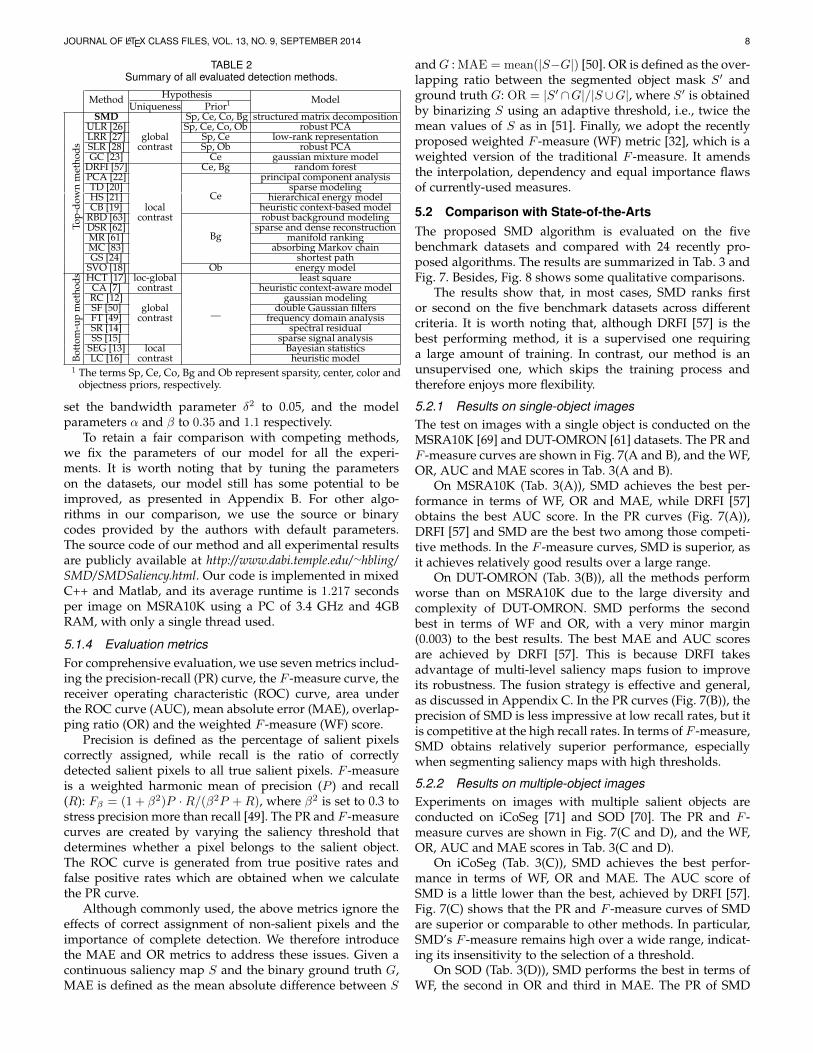
TABLE 2Summary of all evaluated detection methods.

Method Hypothesis ModelUniqueness Prior1

Top-

dow

nm

etho

ds

SMD Sp, Ce, Co, Bg structured matrix decompositionULR [26] Sp, Ce, Co, Ob robust PCALRR [27] global Sp, Ce low-rank representationSLR [28] contrast Sp, Ob robust PCAGC [23] Ce gaussian mixture model

DRFI [57] Ce, Bg random forestPCA [22]

Ce

principal component analysisTD [20] sparse modelingHS [21] hierarchical energy modelCB [19] local heuristic context-based model

RBD [63] contrast

Bg

robust background modelingDSR [62] sparse and dense reconstructionMR [61] manifold rankingMC [83] absorbing Markov chainGS [24] shortest path

SVO [18] Ob energy model

Bott

om-u

pm

etho

ds HCT [17] loc-global

—

least squareCA [7] contrast heuristic context-aware modelRC [12] gaussian modelingSF [50] global double Gaussian filtersFT [49] contrast frequency domain analysisSR [14] spectral residualSS [15] sparse signal analysis

SEG [13] local Bayesian statisticsLC [16] contrast heuristic model

1 The terms Sp, Ce, Co, Bg and Ob represent sparsity, center, color andobjectness priors, respectively.

set the bandwidth parameter δ2 to 0.05, and the modelparameters α and β to 0.35 and 1.1 respectively.

To retain a fair comparison with competing methods,we fix the parameters of our model for all the experi-ments. It is worth noting that by tuning the parameterson the datasets, our model still has some potential to beimproved, as presented in Appendix B. For other algo-rithms in our comparison, we use the source or binarycodes provided by the authors with default parameters.The source code of our method and all experimental resultsare publicly available at http://www.dabi.temple.edu/∼hbling/SMD/SMDSaliency.html. Our code is implemented in mixedC++ and Matlab, and its average runtime is 1.217 secondsper image on MSRA10K using a PC of 3.4 GHz and 4GBRAM, with only a single thread used.

5.1.4 Evaluation metricsFor comprehensive evaluation, we use seven metrics includ-ing the precision-recall (PR) curve, the F -measure curve, thereceiver operating characteristic (ROC) curve, area underthe ROC curve (AUC), mean absolute error (MAE), overlap-ping ratio (OR) and the weighted F -measure (WF) score.

Precision is defined as the percentage of salient pixelscorrectly assigned, while recall is the ratio of correctlydetected salient pixels to all true salient pixels. F -measureis a weighted harmonic mean of precision (P ) and recall(R): Fβ = (1 + β2)P ·R/(β2P +R), where β2 is set to 0.3 tostress precision more than recall [49]. The PR and F -measurecurves are created by varying the saliency threshold thatdetermines whether a pixel belongs to the salient object.The ROC curve is generated from true positive rates andfalse positive rates which are obtained when we calculatethe PR curve.

Although commonly used, the above metrics ignore theeffects of correct assignment of non-salient pixels and theimportance of complete detection. We therefore introducethe MAE and OR metrics to address these issues. Given acontinuous saliency map S and the binary ground truth G,MAE is defined as the mean absolute difference between S

andG : MAE = mean(|S−G|) [50]. OR is defined as the over-lapping ratio between the segmented object mask S′ andground truth G: OR = |S′ ∩G|/|S ∪G|, where S′ is obtainedby binarizing S using an adaptive threshold, i.e., twice themean values of S as in [51]. Finally, we adopt the recentlyproposed weighted F -measure (WF) metric [32], which is aweighted version of the traditional F -measure. It amendsthe interpolation, dependency and equal importance flawsof currently-used measures.

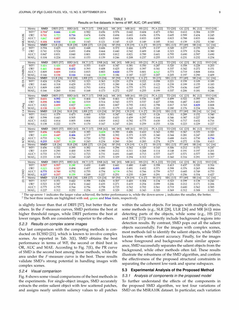
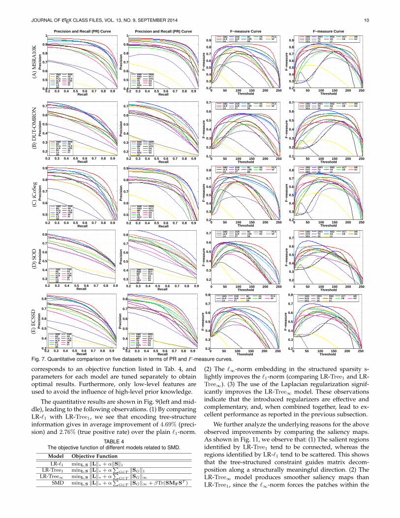
5.2 Comparison with State-of-the-ArtsThe proposed SMD algorithm is evaluated on the fivebenchmark datasets and compared with 24 recently pro-posed algorithms. The results are summarized in Tab. 3 andFig. 7. Besides, Fig. 8 shows some qualitative comparisons.

The results show that, in most cases, SMD ranks firstor second on the five benchmark datasets across differentcriteria. It is worth noting that, although DRFI [57] is thebest performing method, it is a supervised one requiringa large amount of training. In contrast, our method is anunsupervised one, which skips the training process andtherefore enjoys more flexibility.

5.2.1 Results on single-object imagesThe test on images with a single object is conducted on theMSRA10K [69] and DUT-OMRON [61] datasets. The PR andF -measure curves are shown in Fig. 7(A and B), and the WF,OR, AUC and MAE scores in Tab. 3(A and B).

On MSRA10K (Tab. 3(A)), SMD achieves the best per-formance in terms of WF, OR and MAE, while DRFI [57]obtains the best AUC score. In the PR curves (Fig. 7(A)),DRFI [57] and SMD are the best two among those competi-tive methods. In the F -measure curves, SMD is superior, asit achieves relatively good results over a large range.

On DUT-OMRON (Tab. 3(B)), all the methods performworse than on MSRA10K due to the large diversity andcomplexity of DUT-OMRON. SMD performs the secondbest in terms of WF and OR, with a very minor margin(0.003) to the best results. The best MAE and AUC scoresare achieved by DRFI [57]. This is because DRFI takesadvantage of multi-level saliency maps fusion to improveits robustness. The fusion strategy is effective and general,as discussed in Appendix C. In the PR curves (Fig. 7(B)), theprecision of SMD is less impressive at low recall rates, but itis competitive at the high recall rates. In terms of F -measure,SMD obtains relatively superior performance, especiallywhen segmenting saliency maps with high thresholds.

5.2.2 Results on multiple-object imagesExperiments on images with multiple salient objects areconducted on iCoSeg [71] and SOD [70]. The PR and F -measure curves are shown in Fig. 7(C and D), and the WF,OR, AUC and MAE scores in Tab. 3(C and D).

On iCoSeg (Tab. 3(C)), SMD achieves the best perfor-mance in terms of WF, OR and MAE. The AUC score ofSMD is a little lower than the best, achieved by DRFI [57].Fig. 7(C) shows that the PR and F -measure curves of SMDare superior or comparable to other methods. In particular,SMD’s F -measure remains high over a wide range, indicat-ing its insensitivity to the selection of a threshold.

On SOD (Tab. 3(D)), SMD performs the best in terms ofWF, the second in OR and third in MAE. The PR of SMD

http://www.dabi.temple.edu/~hbling/SMD/SMDSaliency.html

http://www.dabi.temple.edu/~hbling/SMD/SMDSaliency.html


TABLE 3Results on five datasets in terms of WF, AUC, OR and MAE.

(A)M

SRA

10K

Metric SMD DRFI [57] RBD [63] HCT [17] DSR [62] MC [83] MR [61] HS [21] PCA [22] TD [20] GC [23] RC [12] SVO [18]WF↑1 0.7042 0.666 0.685 0.582 0.656 0.576 0.642 0.604 0.473 0.561 0.612 0.384 0.339OR↑ 0.741 0.723 0.716 0.674 0.654 0.694 0.693 0.656 0.576 0.605 0.599 0.434 0.245

AUC↑ 0.847 0.857 0.834 0.847 0.825 0.843 0.824 0.833 0.839 0.815 0.788 0.833 0.844MAE↓1 0.104 0.114 0.108 0.143 0.121 0.145 0.125 0.149 0.185 0.161 0.139 0.252 0.340Metric SMD ULR [26] SLR [28] LRR [27] GS [24] SF [50] CB [19] CA [7] SS [15] SEG [13] FT [49] SR [14] LC [16]WF↑ 0.704 0.425 0.601 0.448 0.606 0.372 0.466 0.379 0.137 0.349 0.277 0.155 0.345OR↑ 0.741 0.524 0.691 0.494 0.664 0.440 0.542 0.409 0.148 0.323 0.379 0.256 0.380

AUC↑ 0.847 0.831 0.840 0.801 0.839 0.812 0.821 0.789 0.601 0.795 0.690 0.597 0.690MAE↓ 0.104 0.224 0.141 0.153 0.139 0.246 0.208 0.237 0.255 0.315 0.231 0.232 0.234

(B)D

UT-

OM

RO

N

Metric SMD DRFI [57] RBD [63] HCT [17] DSR [62] MC [83] MR [61] HS [21] PCA [22] TD [20] GC [23] RC [12] SVO [18]WF↑ 0.424 0.424 0.427 0.353 0.419 0.347 0.381 0.350 0.287 0.320 0.358 0.228 0.203OR↑ 0.441 0.444 0.432 0.393 0.408 0.425 0.420 0.397 0.341 0.337 0.342 0.272 0.151

AUC↑ 0.809 0.839 0.814 0.815 0.803 0.820 0.779 0.801 0.827 0.773 0.719 0.808 0.816MAE↓ 0.166 0.138 0.144 0.164 0.139 0.186 0.187 0.227 0.207 0.205 0.197 0.290 0.409Metric SMD ULR [26] SLR [28] LRR [27] GS [24] SF [50] CB [19] CA [7] SS [15] SEG [13] FT [49] SR [14] LC [16]WF↑ 0.424 0.254 0.392 0.323 0.363 0.229 0.274 0.222 0.098 0.221 0.159 0.109 0.189OR↑ 0.441 0.318 0.429 0.353 0.372 0.280 0.338 0.245 0.123 0.239 0.199 0.155 0.183

AUC↑ 0.809 0.805 0.822 0.793 0.814 0.778 0.775 0.771 0.612 0.779 0.636 0.607 0.626MAE↓ 0.166 0.260 0.161 0.168 0.173 0.272 0.257 0.255 0.199 0.337 0.206 0.181 0.246

(C)

iCoS

eg


AUC↑ 0.822 0.839 0.827 0.833 0.801 0.807 0.795 0.812 0.798 0.817 0.765 0.829 0.808MAE↓ 0.138 0.139 0.138 0.179 0.153 0.179 0.162 0.176 0.201 0.180 0.176 0.234 0.336Metric SMD LR [26] SLR [28] LRR [27] GS [24] SF [50] CB [19] CA [7] SS [15] SEG [13] FT [49] SR [14] LC [16]WF↑ 0.611 0.379 0.473 0.465 0.519 0.347 0.441 0.315 0.126 0.301 0.289 0.152 0.340OR↑ 0.598 0.443 0.505 0.530 0.520 0.433 0.459 0.297 0.164 0.346 0.387 0.227 0.348

AUC↑ 0.822 0.814 0.805 0.804 0.819 0.812 0.782 0.775 0.630 0.792 0.717 0.632 0.716MAE↓ 0.138 0.222 0.179 0.170 0.167 0.247 0.201 0.259 0.253 0.326 0.223 0.229 0.227

(D)

SOD


AUC↑ 0.733 0.742 0.706 0.720 0.722 0.746 0.709 0.731 0.730 0.688 0.631 0.730 0.734MAE↓ 0.233 0.217 0.229 0.243 0.234 0.260 0.261 0.283 0.274 0.279 0.272 0.326 0.413Metric SMD LR [26] SLR [28] LRR [27] GS [24] SF [50] CB [19] CA [7] SS [15] SEG [13] FT [49] SR [14] LC [16]WF↑ 0.456 0.322 0.395 0.382 0.416 0.296 0.362 0.320 0.143 0.306 0.212 0.151 0.247OR↑ 0.419 0.290 0.400 0.393 0.390 0.212 0.311 0.268 0.114 0.148 0.191 0.197 0.201

AUC↑ 0.733 0.713 0.712 0.723 0.731 0.691 0.685 0.713 0.577 0.677 0.571 0.577 0.580MAE↓ 0.233 0.308 0.248 0.245 0.251 0.329 0.294 0.312 0.310 0.360 0.316 0.291 0.317

(E)

ECSS

D


AUC↑ 0.775 0.780 0.752 0.755 0.754 0.779 0.761 0.766 0.759 0.717 0.685 0.749 0.753MAE↓ 0.227 0.217 0.225 0.249 0.227 0.251 0.235 0.269 0.291 0.271 0.256 0.334 0.427Metric SMD ULR [26] SLR [28] LRR [27] GS [24] SF [50] CB [19] CA [7] SS [15] SEG [13] FT [49] SR [14] LC [16]WF↑ 0.517 0.351 0.442 0.398 0.436 0.307 0.403 0.304 0.134 0.323 0.199 0.138 0.242OR↑ 0.523 0.347 0.474 0.442 0.435 0.271 0.419 0.254 0.099 0.206 0.212 0.171 0.206

AUC↑ 0.775 0.755 0.764 0.756 0.758 0.725 0.762 0.702 0.561 0.719 0.600 0.562 0.585MAE↓ 0.227 0.312 0.252 0.254 0.255 0.329 0.282 0.343 0.320 0.369 0.312 0.308 0.332

1 The up-arrow ↑ indicates the larger value achieved, the better performance is, while the down-arrow ↓ indicates the smaller, the better.2 The best three results are highlighted with red, green and blue fonts, respectively.

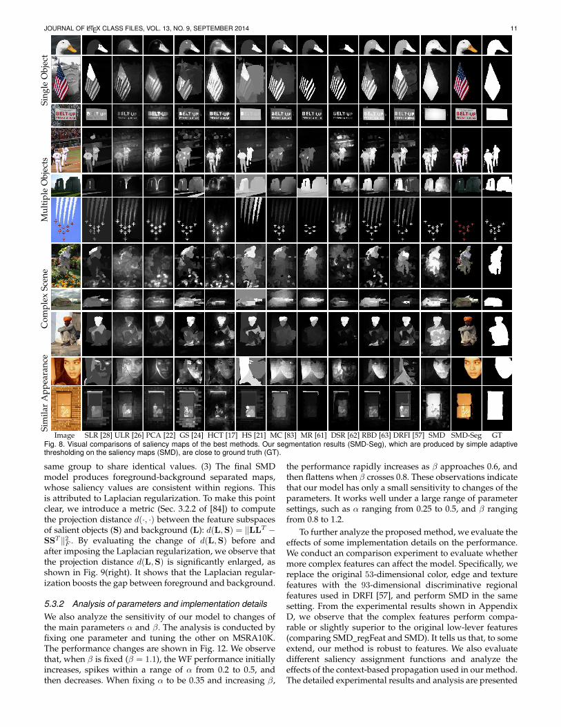
is slightly lower than that of DRFI [57], but better than theothers. In the F -measure curves, SMD performs the best athigher threshold ranges, while DRFI performs the best atlower ranges. Both are consistently superior to the others.5.2.3 Results on complex scene imagesOur last comparison with the competing methods is con-ducted on ECSSD [21], which is known to involve complexscenes. As reported in Tab. 3(E), SMD obtains the bestperformance in terms of WF, the second or third best inOR, AUC and MAE. According to Fig. 7(E), the PR curveof SMD is the second best among those methods, while thearea under the F -measure curve is the best. These resultsvalidate SMD’s strong potential in handling images withcomplex scenes.5.2.4 Visual comparisonFig. 8 shows some visual comparisons of the best methods inthe experiments. For single-object images, SMD accuratelyextracts the entire salient object with few scattered patches,and assigns nearly uniform saliency values to all patches

within the salient objects. For images with multiple objects,some methods (e.g., SLR [28], ULR [26] and MR [61]) missdetecting parts of the objects, while some (e.g., HS [21]and HCT [17]) incorrectly include background regions intodetection results. By contrast, SMD pops out all the salientobjects successfully. For the images with complex scenes,most methods fail to identify the salient objects, while SMDlocates them with decent accuracy. Finally, for the imageswhose foreground and background share similar appear-ance, SMD successfully separates the salient objects from thebackground, while other methods often fail. These resultsillustrate the robustness of the SMD algorithm, and confirmthe effectiveness of the proposed structural constraints inseparating the coherent low-rank and sparse subspaces.

5.3 Experimental Analysis of the Proposed Method5.3.1 Analysis of components in the proposed modelTo further understand the effects of the components inthe proposed SMD algorithm, we test four variations ofSMD on the MSRA10K dataset. In particular, each variation


0.2 0.3 0.4 0.5 0.6 0.7 0.8 0.90.4

0.5

0.6

0.7

0.8

0.9

1

Recall

Pre

cisi

on

Precision and Recall (PR) Curve

SMD DSRMC HSPCA ULRSLR LRRRC SFCA FTSR

(A)M

SRA

10K

0.2 0.3 0.4 0.5 0.6 0.7 0.8 0.90.4

0.5

0.6

0.7

0.8

0.9

1

Recall

Pre

cisi

on

Precision and Recall (PR) Curve

SMD DRFIRBD HCTMR SVOTD GSCB GCSEG SSLC

0 50 100 150 200 2500.2

0.3

0.4

0.5

0.6

0.7

0.8

0.9

Threshold

F−m

easu

re

F−measure Curve

SMD DSR MC HS PCAULR SLR LRR RC SFCA FT SR

0 50 100 150 200 2500.2

0.3

0.4

0.5

0.6

0.7

0.8

0.9

Threshold

F−m

easu

re

F−measure Curve

SMD DRFI RBD HCT MRSVO TD GS CB GCSEG SS LC

0.2 0.3 0.4 0.5 0.6 0.7 0.8 0.9

0.2

0.3

0.4

0.5

0.6

0.7

Recall

Pre

cisi

on


(B)

DU

T-O

MR

ON

0.2 0.3 0.4 0.5 0.6 0.7 0.8 0.9

0.2

0.3

0.4

0.5

0.6

0.7

Recall

Pre

cisi

on


0 50 100 150 200 2500.1

0.2

0.3

0.4

0.5

0.6

0.7

Threshold

F−m

easu

re


0 50 100 150 200 2500.1

0.2

0.3

0.4

0.5

0.6

0.7

Threshold

F−m

easu

re


0.2 0.3 0.4 0.5 0.6 0.7 0.8 0.9

0.5

0.6

0.7

0.8

0.9

Recall

Pre

cisi

on


(C)i

CoS

eg

0.2 0.3 0.4 0.5 0.6 0.7 0.8 0.9

0.5

0.6

0.7

0.8

0.9

Recall

Pre

cisi

on


0 50 100 150 200 2500.2

0.3

0.4

0.5

0.6

0.7

0.8

Threshold

F−m

easu

re


0 50 100 150 200 2500.2

0.3

0.4

0.5

0.6

0.7

0.8

Threshold

F−m

easu

re


0.2 0.3 0.4 0.5 0.6 0.7 0.8 0.9

0.3

0.4

0.5

0.6

0.7

0.8

Recall

Pre

cisi

on


(D)

SOD

0.2 0.3 0.4 0.5 0.6 0.7 0.8 0.9

0.3

0.4

0.5

0.6

0.7

0.8

Recall

Pre

cisi

on


0 50 100 150 200 250

0.2

0.3

0.4

0.5

0.6

0.7

Threshold

F−m

easu

re


0 50 100 150 200 250

0.2

0.3

0.4

0.5

0.6

0.7

ThresholdF

−mea

sure


0.2 0.3 0.4 0.5 0.6 0.7 0.8 0.90.3

0.4

0.5

0.6

0.7

0.8

Recall

Pre

cisi

on


(E)E

CSS

D

0.2 0.3 0.4 0.5 0.6 0.7 0.8 0.90.3

0.4

0.5

0.6

0.7

0.8

Recall

Pre

cisi

on


0 50 100 150 200 2500.2

0.3

0.4

0.5

0.6

0.7

0.8

Threshold

F−m

easu

re


0 50 100 150 200 2500.2

0.3

0.4

0.5

0.6

0.7

0.8

Threshold

F−m

easu

re


Fig. 7. Quantitative comparison on five datasets in terms of PR and F -measure curves.

corresponds to an objective function listed in Tab. 4, andparameters for each model are tuned separately to obtainoptimal results. Furthermore, only low-level features areused to avoid the influence of high-level prior knowledge.

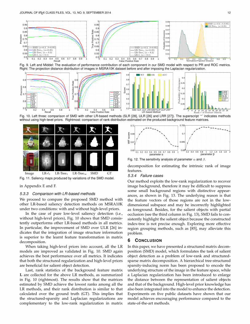
The quantitative results are shown in Fig. 9(left and mid-dle), leading to the following observations. (1) By comparingLR-`1 with LR-Tree1, we see that encoding tree-structureinformation gives in average improvement of 4.69% (preci-sion) and 2.76% (true positive rate) over the plain `1-norm.

TABLE 4The objective function of different models related to SMD.

Model Objective FunctionLR-`1 minL,S ‖L‖∗ + α‖S‖1

LR-Tree1 minL,S ‖L‖∗ + α∑

G∈T ‖SG‖1LR-Tree∞ minL,S ‖L‖∗ + α

∑G∈T ‖SG‖∞

SMD minL,S ‖L‖∗ + α∑

G∈T ‖SG‖∞ + βTr(SMFST )

(2) The `∞-norm embedding in the structured sparsity s-lightly improves the `1-norm (comparing LR-Tree1 and LR-Tree∞). (3) The use of the Laplacian regularization signif-icantly improves the LR-Tree∞ model. These observationsindicate that the introduced regularizers are effective andcomplementary, and, when combined together, lead to ex-cellent performance as reported in the previous subsection.

We further analyze the underlying reasons for the aboveobserved improvements by comparing the saliency maps.As shown in Fig. 11, we observe that: (1) The salient regionsidentified by LR-Tree1 tend to be connected, whereas theregions identified by LR-`1 tend to be scattered. This showsthat the tree-structured constraint guides matrix decom-position along a structurally meaningful direction. (2) TheLR-Tree∞ model produces smoother saliency maps thanLR-Tree1, since the `∞-norm forces the patches within the


Sing

leO

bjec

tM

ulti

ple

Obj

ects

Com

plex

Scen

eSi

mila

rA

ppea

ranc

e

Image SLR [28] ULR [26] PCA [22] GS [24] HCT [17] HS [21] MC [83] MR [61] DSR [62] RBD [63] DRFI [57] SMD SMD-Seg GTFig. 8. Visual comparisons of saliency maps of the best methods. Our segmentation results (SMD-Seg), which are produced by simple adaptivethresholding on the saliency maps (SMD), are close to ground truth (GT).

same group to share identical values. (3) The final SMDmodel produces foreground-background separated maps,whose saliency values are consistent within regions. Thisis attributed to Laplacian regularization. To make this pointclear, we introduce a metric (Sec. 3.2.2 of [84]) to computethe projection distance d(·, ·) between the feature subspacesof salient objects (S) and background (L): d(L,S) = ‖LLT −SST ‖2F . By evaluating the change of d(L,S) before andafter imposing the Laplacian regularization, we observe thatthe projection distance d(L,S) is significantly enlarged, asshown in Fig. 9(right). It shows that the Laplacian regular-ization boosts the gap between foreground and background.

5.3.2 Analysis of parameters and implementation detailsWe also analyze the sensitivity of our model to changes ofthe main parameters α and β. The analysis is conducted byfixing one parameter and tuning the other on MSRA10K.The performance changes are shown in Fig. 12. We observethat, when β is fixed (β = 1.1), the WF performance initiallyincreases, spikes within a range of α from 0.2 to 0.5, andthen decreases. When fixing α to be 0.35 and increasing β,

the performance rapidly increases as β approaches 0.6, andthen flattens when β crosses 0.8. These observations indicatethat our model has only a small sensitivity to changes of theparameters. It works well under a large range of parametersettings, such as α ranging from 0.25 to 0.5, and β rangingfrom 0.8 to 1.2.

To further analyze the proposed method, we evaluate theeffects of some implementation details on the performance.We conduct an comparison experiment to evaluate whethermore complex features can affect the model. Specifically, wereplace the original 53-dimensional color, edge and texturefeatures with the 93-dimensional discriminative regionalfeatures used in DRFI [57], and perform SMD in the samesetting. From the experimental results shown in AppendixD, we observe that the complex features perform compa-rable or slightly superior to the original low-lever features(comparing SMD regFeat and SMD). It tells us that, to someextend, our method is robust to features. We also evaluatedifferent saliency assignment functions and analyze theeffects of the context-based propagation used in our method.The detailed experimental results and analysis are presented


0 0.1 0.2 0.3 0.4 0.5 0.6 0.7 0.8 0.9 10.5

0.55

0.6

0.65

0.7

0.75

0.8

0.85

0.9

0.95

1

Recall

Pre

cisi

on

SMD (α=0.3, β=0.95)LR-Tree∞ (α=0.25)LR-Tree1 (α= 0.3)LR-1 (α= 0.1)

0 0.1 0.2 0.3 0.4 0.5 0.6 0.7 0.8 0.9 10.5

0.55

0.6

0.65

0.7

0.75

0.8

0.85

0.9

0.95

1

False Positive Rate

Tru

e P

ositi

ve R

ate

SMD (α=0.3, β=0.95)LR-Tree∞ (α=0.25)LR-Tree1 (α= 0.3)LR-1 (α= 0.1)

0 0.1 0.2 0.3 0.4 0.5 0.6 0.7 0.8 0.9 10

0.01

0.02

0.03

0.04

0.05

0.06

0.07

0.08

0.09

Normalized Pojection Distance

Pro

babi

lity

of O

ccur

ence

SMD (α=0.3, β=0.95)LR-Tree∞ (α=0.25)

Fig. 9. Left and Middel: The evaluation of performance contribution of each component in our SMD model with respect to PR and ROC metrics.Right: The projection distance distribution of images in MSRA10K dataset before and after imposing the Laplacian regularization.

0 0.2 0.4 0.6 0.8 10.5

0.6

0.7

0.8

0.9

1

Recall

Pre

cisi

on

SMDSMD*SLRSLR*ULRULR*LRRLRR*

0 0.2 0.4 0.6 0.8 10.5

0.6

0.7

0.8

0.9

1

False Positive Rate

Tru

e P

osi

tive R

ate

SMDSMD*SLRSLR*ULRULR*LRRLRR*

SMD SLR ULR LRR SMD*SLR*ULR*LRR*0.2

0.3

0.4

0.5

0.6

0.7

0.8

0.9

LR−based Method

Sco

re

WF OR AUC

2 4 6 8 10 12 14 16 18 20 22 240

0.05

0.1

0.15

0.2

0.25

0.3

Rank r of Feature Matrix

Probab

ilityof

Occurence

LRRULRSLRSMDGT

Fig. 10. Left three: comparison of SMD with other LR-based methods (SLR [28], ULR [26] and LRR [27]). The superscript ‘∗’ indicates methodswithout using high-level priors. Rightmost: comparison of rank distribution estimated on the produced background feature matrices.

Image LR-`1 LR-Tree1 LR-Tree∞ SMD GTFig. 11. Saliency maps produced by variations of the SMD model.

in Appendix E and F.

5.3.3 Comparison with LR-based methodsWe proceed to compare the proposed SMD method withother LR-based saliency detection methods on MSRA10Kunder two conditions: with and without high-level priors.

In the case of pure low-level saliency detection (i.e.,without high-level priors), Fig. 10 shows that SMD consis-tently outperforms other LR-based methods in all metrics.In particular, the improvement of SMD over ULR [26] in-dicates that the integration of image structure informationis superior to the learnt feature transformation in matrixdecomposition.

When taking high-level priors into account, all the LRmodels are improved as validated in Fig. 10. SMD againachieves the best performance over all metrics. It indicatesthat both the structured regularization and high-level priorsare beneficial for salient object detection.

Last, rank statistics of the background feature matrixL are collected for the above LR methods, as summarizedin Fig. 10 (rightmost). The results show that the matricesestimated by SMD achieve the lowest ranks among all theLR methods, and their rank distribution is similar to thatcalculated over the ground truth (GT). This implies thatthe structured-sparsity and Laplacian regularizations arecomplementary to the low-rank regularization in matrix

0.1 0.2 0.3 0.4 0.5 0.6 0.7 0.8 0.9 10.65

0.67

0.69

0.71

parameter α

WF

sco

re

0.2 0.4 0.6 0.8 1 1.2 1.4 1.6 1.8 20.69

0.695

0.7

0.705

parameter β

Fig. 12. The sensitivity analysis of parameter α and β.

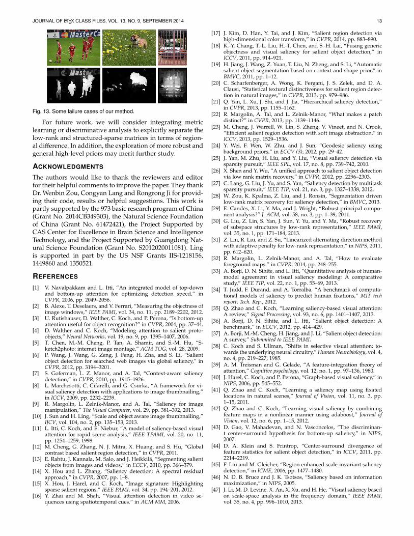
decomposition for estimating the intrinsic rank of imagefeatures.5.3.4 Failure casesOur method exploits the low-rank regularization to recoverimage background, therefore it may be difficult to suppresssome small background regions with distinctive appear-ances, as shown in Fig. 13. The underlying reason is thatthe feature vectors of those regions are not in the low-dimensional subspace and may be incorrectly highlightedas foreground. Besides, for the salient objects with partialocclusion (see the third column in Fig. 13), SMD fails to con-sistently highlight the salient object because the constructedindex-tree is not precise enough. Exploring more effectiveregion grouping methods, such as [85], may alleviate thisproblem.

6 CONCLUSION

In this paper, we have presented a structured matrix decom-position (SMD) model, which formulates the task of salientobject detection as a problem of low-rank and structured-sparse matrix decomposition. A hierarchical tree-structuredsparsity-inducing norm has been proposed to encode theunderlying structure of the image in the feature space, whilea Laplacian regularization has been introduced to enlargethe distance between the representation of salient objectsand that of the background. High-level prior knowledge hasalso been integrated into the model to enhance the detection.Experiments on five public datasets have shown that ourmodel achieves encouraging performance compared to thestate-of-the-art methods.


Fig. 13. Some failure cases of our method.

For future work, we will consider integrating metriclearning or discriminative analysis to explicitly separate thelow-rank and structured-sparse matrices in terms of region-al difference. In addition, the exploration of more robust andgeneral high-level priors may merit further study.

ACKNOWLEDGMENTS

The authors would like to thank the reviewers and editorfor their helpful comments to improve the paper. They thankDr. Wenbin Zou, Congyan Lang and Rongrong Ji for provid-ing their code, results or helpful suggestions. This work ispartly supported by the 973 basic research program of China(Grant No. 2014CB349303), the Natural Science Foundationof China (Grant No. 61472421), the Project Supported byCAS Center for Excellence in Brain Science and IntelligenceTechnology, and the Project Supported by Guangdong Nat-ural Science Foundation (Grant No. S2012020011081). Lingis supported in part by the US NSF Grants IIS-1218156,1449860 and 1350521.

REFERENCES

[1] V. Navalpakkam and L. Itti, “An integrated model of top-downand bottom-up attention for optimizing detection speed,” inCVPR, 2006, pp. 2049–2056.

[2] B. Alexe, T. Deselaers, and V. Ferrari, “Measuring the objectness ofimage windows,” IEEE PAMI, vol. 34, no. 11, pp. 2189–2202, 2012.

[3] U. Rutishauser, D. Walther, C. Koch, and P. Perona, “Is bottom-upattention useful for object recognition?” in CVPR, 2004, pp. 37–44.

[4] D. Walther and C. Koch, “Modeling attention to salient proto-objects,” Neural Networks, vol. 19, no. 9, pp. 1395–1407, 2006.

[5] T. Chen, M.-M. Cheng, P. Tan, A. Shamir, and S.-M. Hu, “S-ketch2photo: internet image montage,” ACM TOG, vol. 28, 2009.

[6] P. Wang, J. Wang, G. Zeng, J. Feng, H. Zha, and S. Li, “Salientobject detection for searched web images via global saliency,” inCVPR, 2012, pp. 3194–3201.

[7] S. Goferman, L. Z. Manor, and A. Tal, “Context-aware saliencydetection,” in CVPR, 2010, pp. 1915–1926.

[8] L. Marchesotti, C. Cifarelli, and G. Csurka, “A framework for vi-sual saliency detection with applications to image thumbnailing,”in ICCV, 2009, pp. 2232–2239.

[9] R. Margolin, L. Zelnik-Manor, and A. Tal, “Saliency for imagemanipulation,” The Visual Computer, vol. 29, pp. 381–392, 2013.

[10] J. Sun and H. Ling, “Scale and object aware image thumbnailing,”IJCV, vol. 104, no. 2, pp. 135–153, 2013.

[11] L. Itti, C. Koch, and E. Niebur, “A model of saliency-based visualattention for rapid scene analysis,” IEEE TPAMI, vol. 20, no. 11,pp. 1254–1259, 1998.

[12] M. Cheng, G. Zhang, N. J. Mitra, X. Huang, and S. Hu, “Globalcontrast based salient region detection,” in CVPR, 2011.

[13] E. Rahtu, J. Kannala, M. Salo, and J. Heikkila, “Segmenting salientobjects from images and videos,” in ECCV, 2010, pp. 366–379.

[14] X. Hou and L. Zhang, “Saliency detection: A spectral residualapproach,” in CVPR, 2007, pp. 1–8.

[15] X. Hou, J. Harel, and C. Koch, “Image signature: Highlightingsparse salient regions,” IEEE PAMI, vol. 34, pp. 194–201, 2012.

[16] Y. Zhai and M. Shah, “Visual attention detection in video se-quences using spatiotemporal cues.” in ACM MM, 2006.

[17] J. Kim, D. Han, Y. Tai, and J. Kim, “Salient region detection viahigh-dimensional color transform,” in CVPR, 2014, pp. 883–890.

[18] K.-Y. Chang, T.-L. Liu, H.-T. Chen, and S.-H. Lai, “Fusing genericobjectness and visual saliency for salient object detection,” inICCV, 2011, pp. 914–921.

[19] H. Jiang, J. Wang, Z. Yuan, T. Liu, N. Zheng, and S. Li, “Automaticsalient object segmentation based on context and shape prior,” inBMVC, 2011, pp. 1–12.

[20] C. Scharfenberger, A. Wong, K. Fergani, J. S. Zelek, and D. A.Clausi, “Statistical textural distinctiveness for salient region detec-tion in natural images,” in CVPR, 2013, pp. 979–986.

[21] Q. Yan, L. Xu, J. Shi, and J. Jia, “Hierarchical saliency detection,”in CVPR, 2013, pp. 1155–1162.

[22] R. Margolin, A. Tal, and L. Zelnik-Manor, “What makes a patchdistinct?” in CVPR, 2013, pp. 1139–1146.

[23] M. Cheng, J. Warrell, W. Lin, S. Zheng, V. Vineet, and N. Crook,“Efficient salient region detection with soft image abstraction,” inICCV, 2013, pp. 1529–1536.

[24] Y. Wei, F. Wen, W. Zhu, and J. Sun, “Geodesic saliency usingbackground priors,” in ECCV (3), 2012, pp. 29–42.

[25] J. Yan, M. Zhu, H. Liu, and Y. Liu, “Visual saliency detection viasparsity pursuit,” IEEE SPL, vol. 17, no. 8, pp. 739–742, 2010.

[26] X. Shen and Y. Wu, “A unified approach to salient object detectionvia low rank matrix recovery,” in CVPR, 2012, pp. 2296–2303.

[27] C. Lang, G. Liu, J. Yu, and S. Yan, “Saliency detection by multitasksparsity pursuit,” IEEE TIP, vol. 21, no. 3, pp. 1327–1338, 2012.

[28] W. Zou, K. Kpalma, Z. Liu, and J. Ronsin, “Segmentation drivenlow-rank matrix recovery for saliency detection,” in BMVC, 2013.

[29] E. Candes, X. Li, Y. Ma, and J. Wright, “Robust principal compo-nent analysis?” J. ACM, vol. 58, no. 3, pp. 1–39, 2011.

[30] G. Liu, Z. Lin, S. Yan, J. Sun, Y. Yu, and Y. Ma, “Robust recoveryof subspace structures by low-rank representation,” IEEE PAMI,vol. 35, no. 1, pp. 171–184, 2013.

[31] Z. Lin, R. Liu, and Z. Su, “Linearized alternating direction methodwith adaptive penalty for low-rank representation,” in NIPS, 2011,pp. 612–620.

[32] R. Margolin, L. Zelnik-Manor, and A. Tal, “How to evaluateforeground maps.” in CVPR, 2014, pp. 248–255.

[33] A. Borji, D. N. Sihite, and L. Itti, “Quantitative analysis of human-model agreement in visual saliency modeling: A comparativestudy,” IEEE TIP, vol. 22, no. 1, pp. 55–69, 2013.

[34] T. Judd, F. Durand, and A. Torralba, “A benchmark of computa-tional models of saliency to predict human fixations,” MIT techreport, Tech. Rep., 2012.

[35] Q. Zhao and C. Koch, “Learning saliency-based visual attention:A review,” Signal Processing, vol. 93, no. 6, pp. 1401–1407, 2013.

[36] A. Borji, D. N. Sihite, and L. Itti, “Salient object detection: Abenchmark,” in ECCV, 2012, pp. 414–429.

[37] A. Borji, M.-M. Cheng, H. Jiang, and J. Li, “Salient object detection:A survey,” Submmited to IEEE PAMI.

[38] C. Koch and S. Ullman, “Shifts in selective visual attention: to-wards the underlying neural circuitry,” Human Neurobiology, vol. 4,no. 4, pp. 219–227, 1985.

[39] A. M. Treisman and G. Gelade, “A feature-integration theory ofattention,” Cognitive psychology, vol. 12, no. 1, pp. 97–136, 1980.

[40] J. Harel, C. Koch, and P. Perona, “Graph-based visual saliency,” inNIPS, 2006, pp. 545–552.

[41] Q. Zhao and C. Koch, “Learning a saliency map using fixatedlocations in natural scenes,” Journal of Vision, vol. 11, no. 3, pp.1–15, 2011.

[42] Q. Zhao and C. Koch, “Learning visual saliency by combiningfeature maps in a nonlinear manner using adaboost,” Journal ofVision, vol. 12, no. 6, pp. 1–15, 2012.

[43] D. Gao, V. Mahadevan, and N. Vasconcelos, “The discriminan-t center-surround hypothesis for bottom-up saliency,” in NIPS,2007.

[44] D. A. Klein and S. Frintrop, “Center-surround divergence offeature statistics for salient object detection,” in ICCV, 2011, pp.2214–2219.

[45] F. Liu and M. Gleicher, “Region enhanced scale-invariant saliencydetection,” in ICME, 2006, pp. 1477–1480.

[46] N. D. B. Bruce and J. K. Tsotsos, “Saliency based on informationmaximization,” in NIPS, 2005.

[47] J. Li, M. D. Levine, X. An, X. Xu, and H. He, “Visual saliency basedon scale-space analysis in the frequency domain,” IEEE PAMI,vol. 35, no. 4, pp. 996–1010, 2013.


[48] T. Liu, Z. Yuan, J. Sun, J. Wang, N. Zheng, X. Tang, and H. Shum,“Learning to detect a salient object,” IEEE PAMI, vol. 33, 2011.

[49] R. Achanta, S. Hemami, F. Estrada, and S. Susstrunk, “Frequency-tuned salient region detection,” in CVPR, 2009, pp. 1597–1604.

[50] F. Perazzi, P. Krahenbuhl, Y. Pritch, and A. Hornung, “Saliencyfilters: Contrast based filtering for salient region detection,” inCVPR, 2012, pp. 733–740.

[51] X. Li, Y. Li, C. Shen, A. R. Dick, and A. van den Hengel, “Contex-tual hypergraph modeling for salient object detection,” in ICCV,2013, pp. 3328–3335.

[52] Y. Niu, Y. Geng, X. Li, and F. Liu, “Leveraging stereopsis forsaliency analysis,” in CVPR, 2012, pp. 454–461.

[53] H. Peng, B. Li, W. Xiong, W. Hu, and R. Ji, “RGBD salient objectdetection: A benchmark and algorithms,” in ECCV, 2014, pp. 1–18.

[54] J. Zhang and S. Sclaroff, “Saliency detection: A boolean mapapproach,” in ICCV, 2013, pp. 153–160.

[55] J. Yang and M. Yang, “Top-down visual saliency via joint crf anddictionary learning,” in CVPR, 2012, pp. 2296–2303.

[56] L. Mai, Y. Niu, and F. Liu, “Saliency aggregation: A data-drivenapproach,” in CVPR, 2013, pp. 1131–1138.

[57] H. Jiang, J. Wang, Z. Yuan, Y. Wu, N. Zheng, and S. Li, “Salientobject detection: A discriminative regional feature integrationapproach,” in CVPR, 2013, pp. 1–8.

[58] M. Jiang, J. Xu, and Q. Zhao, “Saliency in crowd,” in ECCV, 2014,pp. 17–32.

[59] S. He, R. W. Lau, W. Liu, Z. Huang, and Q. Yang, “Supercnn:A superpixelwise convolutional neural network for salient objectdetection,” International Journal of Computer Vision, pp. 1–15.

[60] K. Shi, K. Wang, J. Lu, and L. Lin, “PISA: pixelwise image salien-cy by aggregating complementary appearance contrast measureswith spatial priors,” in CVPR, 2013, pp. 2115–2122.

[61] C. Yang, L. Zhang, H. Lu, X. Ruan, and M.-H. Yang, “Saliencydetection via graph-based manifold ranking,” in CVPR, 2013, pp.3166–3173.

[62] X. Li, H. Lu, L. Zhang, X. Ruan, and M.-H. Yang, “Saliencydetection via dense and sparse reconstruction,” in ICCV, 2013, pp.2976–2983.

[63] W. Zhu, S. Liang, Y. Wei, and J. Sun, “Saliency optimization fromrobust background detection,” in CVPR, 2014, pp. 2814–2821.

[64] P. Jiang, H. Ling, J. Yu, and J. Peng, “Salient region detection byufo: Uniqueness, focusness and objectness,” in ICCV, 2013, pp.1976–1983.

[65] Y. Jia and M. Han, “Category-independent object-level saliencydetection,” in ICCV, 2013, pp. 1761–1768.

[66] T. Judd, K. A. Ehinger, F. Durand, and A. Torralba, “Learning topredict where humans look,” in ICCV, 2009, pp. 2106–2113.

[67] D. Zhou, J. Weston, A. Gretton, O. Bousquet, and B. Scholkopf,“Ranking on data manifolds,” in NIPS, 2003.

[68] H. Peng, B. Li, R. Ji, W. Hu, W. Xiong, and C. Lang, “Salient objectdetection via low-rank and structured sparse matrix decomposi-tion,” in AAAI, 2013.

[69] M.-M. Cheng, N. J. Mitra, X. Huang, P. H. S. Torr, and S.-M.Hu, “Global contrast based salient region detection,” IEEE TPAMI,2014.

[70] V. Movahedi and J. H. Elder, “Design and perceptual validation ofperformance measures for salient object segmentation,” in POCV,2010.

[71] D. Batra, A. Kowdle, D. Parikh, J. Luo, and T. Chen, “Interactivelyco-segmentating topically related images with intelligent scribbleguidance,” IJCV, vol. 93, no. 3, pp. 273–292, 2011.

[72] J. Ye, “Generalized low rank approximations of matrices,” inICML, 2004.

[73] S. Lu, X. Ren, and F. Liu, “Depth enhancement via low-rank matrixcompletion.” in CVPR, 2014, pp. 3390–3397.

[74] J. Liu and J. Ye, “Moreau-yosida regularization for grouped treestructure learning,” in NIPS, 2010, pp. 1459–1467.

[75] K. Jia, T. Chan, and Y. Ma, “Robust and practical face recognitionvia structured sparsity,” in ECCV, 2012, pp. 331–344.

[76] D. Cai, X. He, J. Han, and T. S. Huang, “Graph regularizednonnegative matrix factorization for data representation,” IEEEPAMI, vol. 33, no. 8, pp. 1548–1560, 2011.

[77] J. Cai, E. J. Candes, and Z. Shen, “A singular value thresholdingalgorithm for matrix completion,” SIAM Journal on Optimization,vol. 20, no. 4, pp. 1956–1982, 2010.

[78] R. Jenatton, J. Mairal, G. Obozinski, and F. Bach, “Proximal meth-ods for hierarchical sparse coding,” JMLR, vol. 12, pp. 7–24, 2011.

[79] E. P. Simoncelli and W. T. Freeman, “The steerable pyramid: Aflexible architecture for multi-scale derivative computation,” inICIP, 1995, pp. 444–447.

[80] H. G. Feichtinger and T. Strohmer, Gabor analysis and algorithm-s:theory and applications. Springer, 1998.

[81] R. Achanta, A. Shaji, K. Smith, A. Lucchi, P. Fua, and S. Susstrunk,“Slic superpixels compared to state-of-the-art superpixel method-s,” IEEE TPAMI, vol. 34, no. 11, pp. 2274–2282, 2012.

[82] P. Felzenszwalb and D. Huttenlocher, “Efficient graph-based im-age segmentation,” IJCV, vol. 59, no. 2, pp. 167–181, 2004.

[83] B. Jiang, L. Zhang, H. Lu, C. Yang, and M.-H. Yang, “Saliencydetection via absorbing markov chain,” in ICCV, 2013, pp. 65–72.

[84] J. Ham and D. D. Lee, “Grassmann discriminant analysis: aunifying view on subspace-based learning,” in ICML, 2008, pp.376–383.

[85] P. A. Arbelaez, J. Pont-Tuset, J. T. Barron, F. Marques, and J. Malik,“Multiscale combinatorial grouping,” in CVPR, 2014, pp. 328–335.

Houwen Peng received the BE degree fromDalian University of Technology, China, in 2011.Currently, he is a PhD student jointly training inthe Institute of Automation, Chinese Academyof Sciences, and the Department of Computerand Information Science, Temple University. Hisresearch interests include pattern recognition,computer vision, and machine learning.

Bing Li received the Ph.D. degree from the De-partment of Computer Science and Engineer-ing, Beijing Jiaotong University, Beijing, China,in 2009. Currently, he is an associate professorwith the Institute of Automation, Chinese Acade-my of Sciences, Beijing. His research interestsinclude color constancy, visual saliency, and webcontent mining.

Haibin Ling received the BS and MS degreesfrom Peking University, China, in 1997 and 2000,respectively, and the PhD degree from the Uni-versity of Maryland, College Park, in 2006. From2006 to 2007, he worked as a postdoctoral sci-entist at UCLA. In 2008, he joined Temple Uni-versity where he is now an associate professor.His research interests include computer visionand medical image analysis.

Weiming Hu received the PhD degree from theDepartment of Computer Science and Engineer-ing, Zhejiang University in 1998. From 1998 to2000, he was a postdoctoral research fellow withthe Institute of Computer Science and Technolo-gy, Peking University. Currently, he is a professorin the Institute of Automation, Chinese Acade-my of Sciences. His research interests includevisual motion analysis and recognition of webobjectionable information.Weihua Xiong received the Ph.D. degree fromthe Department of Computer Science, SimonFraser University, Vancouver, BC, Canada, in2007. Currently, he is an imaging scientist atOmniVision Technologies Inc.. His research in-terests include color science, computer vision,color image processing, and stereo vision. He isa reviewer, committee member or session chairfor several international conference and journals.

Stephen J. Maybank Stephen J. Maybank re-ceived the BA degree in mathematics from KingsCollege Cambridge in 1976, and the PhD degreein computer science from Birkbeck College, Uni-versity of London in 1988. He is currently a pro-fessor in the Department of Computer Scienceand Information Systems, Birkbeck College. Hisresearch interests include the geometry of mul-tiple images, camera calibration, visual surveil-lance, etc. He is a fellow of the IEEE.

journal of la salient object detection via structured ...sjmaybank/salientobject.pdf · salient...

Documents