at SciVerse ScienceDirect

Journal of Power Sources 224 (2013) 20e27

Contents lists available

Journal of Power Sources

journal homepage: www.elsevier .com/locate/ jpowsour

Advanced mathematical methods of SOC and SOH estimation for lithium-ionbatteries

Dave Andre a,*, Christian Appel a, Thomas Soczka-Guth a, Dirk Uwe Sauer b

aDeutsche ACCUmotive GmbH & Co. KG, 73230 Kirchheim u. Teck (Nabern), Germanyb Institute for Power Electronics and Electrical Drives (ISEA), RWTH Aachen University, 52066 Aachen, Germany

h i g h l i g h t s

< Advanced SOC and SOH estimation of a lithium-ion battery by a Dual Kalman filter in combination with support vector machine.< Feasibility proof and validation by measured drive cycle data.< Estimation accuracy far better than the reported ones (SOC error < 0.5%).< Real-time diagnosis by management system conceivable.

a r t i c l e i n f o

Article history:Received 3 May 2012Received in revised form27 August 2012Accepted 1 October 2012Available online 6 October 2012

Keywords:State of healthLithium-ion batteryState of chargeBattery management systemUnscented Kalman filterSupport vector regression

* Corresponding author. Tel.: þ49 (0)15158605924.E-mail address: dave.andre@daimler.com (D. Andr

0378-7753/$ e see front matter � 2012 Elsevier B.V.http://dx.doi.org/10.1016/j.jpowsour.2012.10.001

a b s t r a c t

Two novel methods to estimate the state of charge (SOC) and state of health (SOH) of a lithium-ionbattery are presented. Based on a detailed deduction, a dual filter consisting of an interaction ofa standard Kalman filter and an Unscented Kalman filter is proposed in order to predict internal batterystates. In addition, a support vector machine (SVM) algorithm is implemented and coupled with the dualfilter. Both methods are verified and validated by cell measurements in form of cycle profiles as well asstorage and cycle ageing tests. A SOC estimation error below 1% and accurate resistance determinationare presented.

� 2012 Elsevier B.V. All rights reserved.

1. Introduction

In automotive applications, the estimation of the actual state ofcharge (SOC) and state of health (SOH) of the battery is rathercrucial to predict e.g. the availability of power and energy inhybrid electric vehicles (HEV) and electric vehicles (EV). Duringlifetime, the resistance as well as the capacity and in consequenceSOC of every lithium-ion cell changes through electrochemicaldegradation processes like electrolyte decomposition or growth ofa solid electrolyte interface (SEI) on the anode surface [1]. Thisvariation is hard to measure directly in a vehicle, but has to beknown for an accurate range and power prediction. Without a SOHcorrection or update by the battery management system (BMS),

e).

All rights reserved.

the driver will experiences an overestimated range or lessacceleration.

Because of this necessity of a reliable SOC and SOH prediction,there were a lot of publications in the last few years. The appli-cation of Kalman filtering can be regarded as a state of the arttechnique. Usually Extended Kalman filtering is used (e.g. Ref. [2]),but also Unscented or Sigma-Point Kalman filtering is utilized (e.g.Ref. [3]).

The use of machine learning techniques, and especially supportvector machines, has grown in popularity over the last few years,not only in SOC and SOH estimation [4e6] but in various applica-tion areas. A good overview of the state-of-art battery prognosticalgorithms is given by Zhang and Lee [7], where not only Kalmanfilters and support vector machines, but also other techniques, suchas neural networks or particle filters are presented.

This paper is based on the master thesis of Christian Appel andpresents a novel method for SOC and SOH prediction using

(i) Calculate state estimate and estimate covarianceprediction (a priori):

D. Andre et al. / Journal of Power Sources 224 (2013) 20e27 21

a standard Kalman filter for linear systems, an Unscented Kalmanfilter and machine learning techniques is presented. Due to itsgeneral structure and design; this approach, demonstrated ata nickel manganese cobalt (NMC) pouch cell, is valid independent ofcell chemistry and design. Even if no direct understanding of theageing mechanism or sources can be gained by such SOH algorithm,information can be collected about the caused degradation ofparticular ageing factors. Thus, the main factors can be identifiedand minimized by an optimized operation strategy on the BMSlater on.

After the introduction and the presentation of the state of the artSOC and SOH estimation, a brief description of the mathematicalmethods used in this approach is given in the second section,followed by the description of the measurements and ageing test.The fourth section describes the implementation of the batterymodel and the application of the mathematical methods andsubsequently the results are presented and discussed.

bxðkþ 1jkÞ ¼ AkbxðkjkÞ þ Bkuk

Pðkþ 1jkÞ ¼ AkPðkjkÞATk þ Qk

(ii) Calculate innovation and innovation covariance:

rkþ1 ¼ zkþ1 � Hkþ1bxðkþ 1jkÞSkþ1 ¼ Hkþ1Pðkþ 1jkÞHT

kþ1 þ Rkþ1

2. Mathematical methods

In this section a description of the mathematical methodsapplied in this study is given. Namely this is a standard Kalmanfilter, an Unscented Kalman filter and the support vectorregression.

(iii) Calculate Kalman gain:

Kkþ1 ¼ Pðkþ 1jkÞHTkþ1S

�1kþ1

(iv) Calculate state estimate and estimate covarianceupdate (a posteriori):

bxðkþ 1jkþ 1Þ ¼ bxðkþ 1jkÞ þ Kkþ1rkþ1Pðkþ 1jkþ 1Þ ¼ Pðkþ 1jkÞ þ Kkþ1Skþ1K

Tkþ1

2.1. Kalman filter for linear systems

The first used technique will be the well-known Kalmanfilter (KF) for linear systems, developed by Kalman in 1960 [8].A good introduction to Kalman filters can be found in Ref. [9].Thus, only a presentation of the applied algorithm is given inthis paper.

A n-dimensional linear dynamic discretized system of a discreterandom process consists of the following:

(i) A process model:

xkþ1 ¼ Akxk þ Bkuk þ vk; (1)

where xk is a discrete random process, which is called state vector,Ak ˛ Rn�n the state transition matrix, Bk ˛ Rn�m the control inputmatrix, uk ˛ Rm a deterministic control vector and vk an uncorre-lated discrete random process, which is called process noise,where:

Qk ¼ EðvkvTk Þ

(ii) An observation model:

zk ¼ Hkxk þwk; (2)

where Hk ˛ Rl�n is the observation matrix and wk an uncorrelateddiscrete random process, which is called measurement noise,where:

Rk ¼ EðwkwTk Þ

Presuming that the following assumptions hold:

EðwkvTj Þ ¼ 0 cj; k (3)

EðwkxTj Þ ¼ 0 for j � k (4)

EðvkxTj Þ ¼ 0 for j � k (5)

Let bxk ¼ bxðkj:kÞ the a posteriori state estimate andPk ¼ P(kjk) be the a posteriori error covariance matrix at timestep k, given measurements up to time step k, then the standardKalman filter equations for the described linear system are thefollowing:

2.2. Unscented Kalman filter

For our purpose a nonlinear extension to the Kalman filter isapplied: the Unscented Kalman filter (UKF), using the unscentedtransformation as described in Ref. [10]. Rather than linearizing thenonlinear functions as in the Extended Kalman filter (EKF), theprobability distribution will be approximated by a certain numberof sigma points and those will be transformed by the nonlinearsystem functions to approximate the mean and covarianceestimate.

The discretized general nonlinear dynamic system has thefollowing form, analogous to the linear systems (1) and (2) andrequiring assumptions (3)e(5) still hold:

(i) Process model:

xkþ1 ¼ fkðxk;uk; vkÞ (6)

(ii) Observation model:

zk ¼ hkðxk;wkÞ (7)

(i) Choose n þ 1 sigma points as follows:

xð0Þ ¼ x ¼ EðxÞxðiÞ ¼ xð0Þ þ � ffiffiffiffiffiffiffiffiffiffiffiffiffiffiffiffiffiffiðnþ kÞPp �T

i ; i ¼ 1;.;n

xðnþiÞ ¼ xð0Þ � � ffiffiffiffiffiffiffiffiffiffiffiffiffiffiffiffiffiffiðnþ kÞPp �Ti ; i ¼ 1;.;n;

where ð ffiffiffiffiffiffiffiffiffiffiffiffiffiffiffiffiffiffiðnþ kÞPp Þi is the ith row of the matrix square rootð ffiffiffiffiffiffiffiffiffiffiffiffiffiffiffiffiffiffiðnþ kÞPp Þ.Weights of the sigma points are chosen as follows:

Wð0Þ ¼ k

nþ k

WðiÞ ¼ 12ðnþ kÞ; i ¼ 1;.;2n

(ii) Calculate state estimate prediction (a priori):

xðiÞðkþ 1jkÞ ¼ f�xðiÞðkjkÞ;uk

�þ vkbxðkþ 1jkÞ ¼ P2ni¼0

WðiÞxðiÞðkþ 1jkÞ

(iii) Calculate estimate covariance prediction (a priori):

Pðkþ 1jkÞ ¼ Qk þX2ni¼0

WðiÞ�xðiÞðkþ 1jkÞ � bxðkþ 1jkÞ

�

��xðiÞðkþ 1jkÞ � bxðkþ 1jkÞ

�T(iv) Calculate innovation:

zðiÞðkþ 1jkÞ ¼ h�xðiÞðkþ 1jkÞ;uk

�þwkbzðkþ 1jkÞ ¼ P2ni¼0

WðiÞzðiÞðkþ 1jkÞ

(v) Calculate Kalman gain:

Pyyðkþ 1jkÞ ¼ Rk þP2ni¼0

WðiÞ�zðiÞðkþ 1jkÞ � bzðkþ 1jkÞ

��zðiÞðkþ 1jkÞ � bzðkþ 1jkÞ

�TPxyðkþ 1jkÞ

¼X2ni¼0

WðiÞ�xðiÞðkþ 1jkÞ � bxðkþ 1jkÞ

��zðiÞðkþ 1jkÞ

� bzðkþ 1jkÞ�T

Kk

¼ Pxyðkþ 1jkÞPyyðkþ 1jkÞ�1

(vi) Calculate state estimate update (a posteriori):

bxðkþ 1jkþ 1Þ ¼ bxðkþ 1jkÞ þ Kk

zk � bzðkþ 1jkÞ

(vii) Calculate estimate covariance update (a posteriori):

Pðkþ 1jkþ 1Þ ¼ Pðkþ 1jkÞ þ KkPyyðkþ 1jkÞKTk

D. Andre et al. / Journal of Power Sources 224 (2013) 20e2722

2.3. Support vector regression

The second method used in this approach is the support vectorregression (SVR). A comprehensive introduction can be found inRef. [11]. Given a set of training data:

fðx1; y1Þ; ðx2; y2Þ;.; ðxn; ynÞg3Rn � R (8)

where xi ˛ Rn are the input parameter vectors and yi ˛ R are thetarget values, the task in the so-called 3-incentive support vectorregression is to find a linear function

f ðxÞ ¼ hw; xi þ b (9)

as flat as possible in the way that the values f(xi) have at most 3

deviation from the targets yi. Introducing “slack variables” xi; x*i to

create a “soft margin” and therefore allowing measurement errorsand be able to cope with otherwise infeasible constraints, leads toa dual optimization problem. Utilizing the KarusheKuhneTucker(KKT) condition, the parameter b in function f(x) can be calcu-lated. Obviously SOC and SOH prediction will not be a linearregression problem, so a method for the nonlinear case is required.Hereby, the idea is to transform the input data nonlinearly ina higher dimensional feature space F:

f : Rn/Fx1fðxÞThe equations in the dual optimization problem are solely

dependent on inner products of the form hxi; xji. Hence in featurespace it is sufficient to know

k�xi; xj

� ¼ �fðxiÞ;f

�xj��

(10)

with a so called kernel function k to represent an inner product infeature space and the nonlinear transformation f has not be knownexplicitly. This is the kernel trick andMercer’s theorem (1909) givesa condition for such functions.

In this study an 3-incentive support vector regression is appliedand Gaussian Kernels of the following form will be used:

kðx; yÞ :¼ exp

� kx� yk2

2s2

!(11)

3. Experiments

In this section a description of the measurements takenfor the present study and details of the used cell type aregiven.

High-energy lithium-ion pouch cells with a graphite anode anda NMC cathode were used. The cells have a nominal voltage of 3.6 Vand a nominal capacity of 10 Ah.

In order to have the chance to validate the subsequent esti-mation, all cells were characterized by electrical parameter tests.Besides a capacity test with a C-rate of one, a pulse powercharacterization profile (PPCP), based on the “Hybrid PulsePower Characterisation Test” of PNGV/FreedomCar and theEUCAR “Open Circuit Voltage and Power Determination Test”[12], is part of this characterization. It consists of a certain pulsepower profile at different SOC steps, from 90%SOC down to 10%SOC in 10%SOC-steps. The pulse power profile procedure can beseen in Table 1.

The SOCeOCV curves, which are later required in the processmodel of filter 2, are obtained from the PPCP measurements as wellas a time-dependent resistance

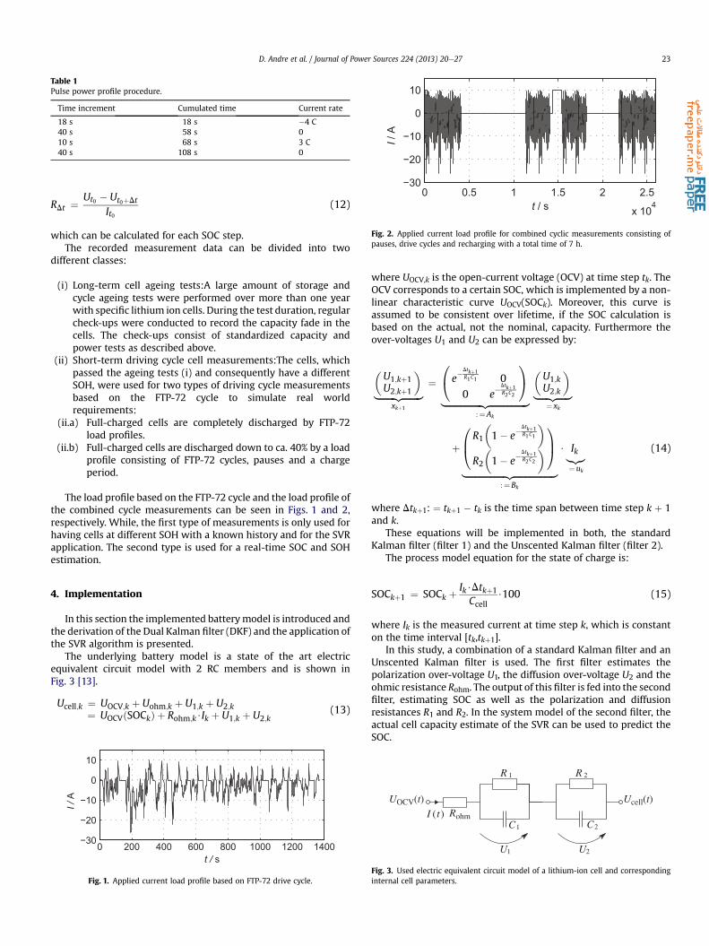
Table 1Pulse power profile procedure.

Time increment Cumulated time Current rate

18 s 18 s �4 C40 s 58 s 010 s 68 s 3 C40 s 108 s 0

0 0.5 1 1.5 2 2.5

x 104

−30

−20

−10

0

10

t / s

I /

A

D. Andre et al. / Journal of Power Sources 224 (2013) 20e27 23

RDt ¼ Ut0 � Ut0þDt

It0(12)

Fig. 2. Applied current load profile for combined cyclic measurements consisting ofpauses, drive cycles and recharging with a total time of 7 h.

which can be calculated for each SOC step.The recorded measurement data can be divided into two

different classes:

(i) Long-term cell ageing tests:A large amount of storage andcycle ageing tests were performed over more than one yearwith specific lithium ion cells. During the test duration, regularcheck-ups were conducted to record the capacity fade in thecells. The check-ups consist of standardized capacity andpower tests as described above.

(ii) Short-term driving cycle cell measurements:The cells, whichpassed the ageing tests (i) and consequently have a differentSOH, were used for two types of driving cycle measurementsbased on the FTP-72 cycle to simulate real worldrequirements:

(ii.a) Full-charged cells are completely discharged by FTP-72load profiles.

(ii.b) Full-charged cells are discharged down to ca. 40% by a loadprofile consisting of FTP-72 cycles, pauses and a chargeperiod.

The load profile based on the FTP-72 cycle and the load profile ofthe combined cycle measurements can be seen in Figs. 1 and 2,respectively. While, the first type of measurements is only used forhaving cells at different SOH with a known history and for the SVRapplication. The second type is used for a real-time SOC and SOHestimation.

4. Implementation

In this section the implemented batterymodel is introduced andthe derivation of the Dual Kalman filter (DKF) and the application ofthe SVR algorithm is presented.

The underlying battery model is a state of the art electricequivalent circuit model with 2 RC members and is shown inFig. 3 [13].

Ucell;k ¼ UOCV;k þ Uohm;k þ U1;k þ U2;k¼ UOCVðSOCkÞ þ Rohm;k$Ik þ U1;k þ U2;k

(13)

0 200 400 600 800 1000 1200 1400−30

−20

−10

0

10

t / s

I / A

Fig. 1. Applied current load profile based on FTP-72 drive cycle.

where UOCV,k is the open-current voltage (OCV) at time step tk. TheOCV corresponds to a certain SOC, which is implemented by a non-linear characteristic curve UOCV(SOCk). Moreover, this curve isassumed to be consistent over lifetime, if the SOC calculation isbased on the actual, not the nominal, capacity. Furthermore theover-voltages U1 and U2 can be expressed by:

U1;kþ1U2;kþ1

|fflfflfflfflfflfflfflffl{zfflfflfflfflfflfflfflffl}

xkþ1

¼0@ e�

Dtkþ1R1C1 0

0 e�Dtkþ1R2C2

1A|fflfflfflfflfflfflfflfflfflfflfflfflfflfflfflfflffl{zfflfflfflfflfflfflfflfflfflfflfflfflfflfflfflfflffl}

:¼Ak

U1;kU2;k

|fflfflfflfflffl{zfflfflfflfflffl}

¼ xk

þ

0B@R1

1� e�

Dtkþ1R1C1

R2

1� e�

Dtkþ1R2C2

1CA

|fflfflfflfflfflfflfflfflfflfflfflfflfflfflfflfflfflffl{zfflfflfflfflfflfflfflfflfflfflfflfflfflfflfflfflfflffl}:¼Bk

$ Ik|{z}¼uk

(14)

where Dtkþ1: ¼ tkþ1 � tk is the time span between time step k þ 1and k.

These equations will be implemented in both, the standardKalman filter (filter 1) and the Unscented Kalman filter (filter 2).

The process model equation for the state of charge is:

SOCkþ1 ¼ SOCk þIk$Dtkþ1Ccell

$100 (15)

where Ik is the measured current at time step k, which is constanton the time interval [tk,tkþ1].

In this study, a combination of a standard Kalman filter and anUnscented Kalman filter is used. The first filter estimates thepolarization over-voltage U1, the diffusion over-voltage U2 and theohmic resistance Rohm. The output of this filter is fed into the secondfilter, estimating SOC as well as the polarization and diffusionresistances R1 and R2. In the system model of the second filter, theactual cell capacity estimate of the SVR can be used to predict theSOC.

Rohm

R 1 R 2

C2C1

U1 U2

I (t)

UOCV(t) Ucell(t)

Fig. 3. Used electric equivalent circuit model of a lithium-ion cell and correspondinginternal cell parameters.

Table 2Equations for filter 1 (KF).

State vectorxk ¼ ð U1;k

U2;kRohm;k

ÞControl input uk ¼ IkObservation zk ¼ Ucell,k � UOCV,k

Process model xkþ1 ¼ Ak$xk þ Bk$ukObservation model zk ¼ (1 1 Ik)$xk

Fig. 4. Design of the dual Kalman filter with estimated states, required inputs andinteractions of the filters.

Table 4Data structure and set parameters of the support vector regression.

D. Andre et al. / Journal of Power Sources 224 (2013) 20e2724

The motivation for this Dual Kalman filter is based on threeadvantages:

� Decoupling of estimations, thus reduction of interactions andavoiding of building-ups of a filter

� Separation of variables, which cannot be estimated by a singlefilter

� Reduction of computation efforts, since two filters of lowerdimensions are faster than one higher dimensional one [14]

Both filters use the input signal current and the measured cellvoltage. Measurement data were obtained by the previouslydescribed driving cycle tests to simulate real world requirements.Therefore the dual filter can be used online, that means e.g. it can beimplemented in the battery management system to predict thepower and energy availability.

The equations for both filters can be found in Tables 2 and 3,respectively. The time constants s1 ¼ R1C1 and s2 ¼ R2C2 wereassumed to be constant in both filters. This assumptions was rathermade than keeping the capacities C1 and C2 constant, because of thefitting results and robustness considerations. The dual filter layoutcan be found in Fig. 4.

The actual cell capacity is also required in the process model ofthe second (Unscented) Kalman filter. It is possible to take thenominal capacity or any other recent measurement result. In thisstudy, the actual relative cell capacity Crel,k ¼ Ccell,k/CBOT is esti-mated by 3-SVR, where CBOT is the begin-of-test (BOT) capacity, andserves as an input value for the model parameter in the secondKalman filter. The data for the SVR was obtained from the long-term cell ageing tests (i).

The composition of the input vector can be seen in Table 4 withan additional scaling to [�1,1] for temperatures and [0,1] for theother features [15].

Multiple data vectors were created for every check-up of everycell, such that every time interval between a check-up and allprevious check-ups including the BOT measurement is accounted.

Table 3Equations for filter 2 (UKF).

xk ¼ ð SOCkR1;kR2;k

Þuk ¼ Ik

zk ¼ Ucell;k � U1;k � U2;k � Uohm;k

U1;kU2;k

!

xkþ1 ¼ xk þ

0BBBB@Dtkþ1Ccell00

1CCCCA$uk

zk ¼

0BBBB@UOCVðx1;kÞ

U1;k�1$e�Dtk

s1 þ x2;k$1� e�

Dtks1

$Ik�1

U2;k�1$e�Dtk

s2 þ x3;k$1� e�

Dtks2

$Ik�1

1CCCCA

In this way a number of 1899 training vectors and 566 testingvectors was obtained.

The choice of the required 3-SVR parameters can be seen inTable 4, where the value of 3was chosen because of the expectedmeasurement error and cell spread. The kernel function parameter~s ¼ 1=2s2 and the regularization constant Cwere obtained by gridsearch and 5-fold cross validation [15] based on the training data.

The SVR part is used offline and the ideas are that new trainingdata can be fed into the model e.g. regularly when a full charge isperformed or at regular services.

In addition, the SVR could also be used to obtain initial values forthe resistances estimated in the DKF or to deliver estimates of thestate of health on its own.

A very interesting further application of the SVR would be todetermine the parameters of an equation describing the ageing orthe lifetime instead of predicting the capacity directly. A possibleequation would be e.g:

Cactual ¼ CBOL$�100� a$tb � h$Ahthroughput

(16)

Variable Description

(a) Composition of the data vectorsInput vectorCrel,t1 Relative cell capacity at time t1Tmin Minimal temperatureTmax Maximal temperatured ¼ t2�t1 Time spanImean Mean current rateq Amount of charge and dischargeSOCmax Maximal SOCDSOC SOC liftTarget valueCrel;t2 Relative cell capacity at time t2

SVR parameter Value(b) Initialised parametersKernel function k(x,y)

exp

� kx� yk2

2s2

!where 1/2s2 ¼ 2.9

3 0.005C 60

D. Andre et al. / Journal of Power Sources 224 (2013) 20e27 25

to describe the capacity fade over calendar and cycle life. Thedependency of the parameters on the operation conditions couldnow be obtained by the SVR. This approach was tested and showedalso very satisfying results for the training as well as the validationwith unknown ageing conditions. Two main advantages can befound for this indirect approach. First, measurements inaccuraciesare compensated and the estimation is more robust againstmeasurement errors or noise. Second, by obtaining these parame-ters an additional prognosis is possible. Especially, if a large number

0 0.5 1 1.5 2

x 104

2

3

4

5

6

7

8x 10

−3

Roh

m /

mΩ

0 0.5 1 1.5 2

x 104

−10

−5

0

5x 10

−3

U1 /

V

0 0.5 1 1.5 2

x 104

−0.03

−0.025

−0.02

−0.015

−0.01

−0.005

0

t / s

U2

/V

# 1# 2# 3# 4

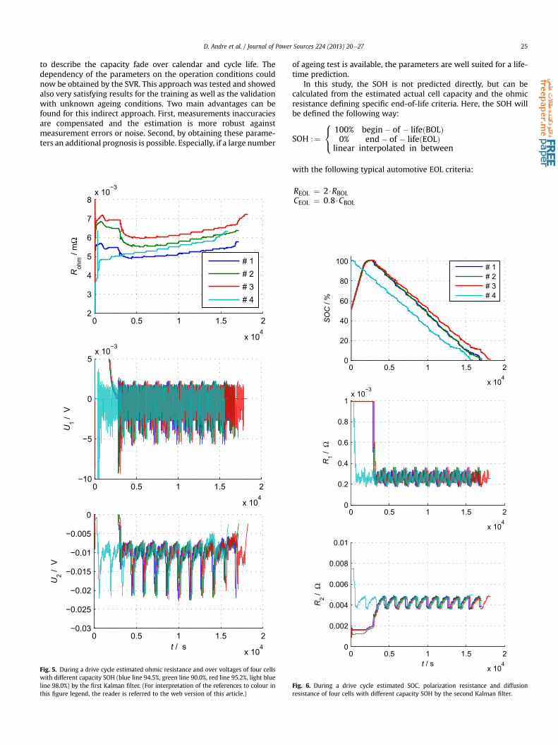
Fig. 5. During a drive cycle estimated ohmic resistance and over voltages of four cellswith different capacity SOH (blue line 94.5%, green line 90.0%, red line 95.2%, light blueline 98.0%) by the first Kalman filter. (For interpretation of the references to colour inthis figure legend, the reader is referred to the web version of this article.)

of ageing test is available, the parameters are well suited for a life-time prediction.

In this study, the SOH is not predicted directly, but can becalculated from the estimated actual cell capacity and the ohmicresistance defining specific end-of-life criteria. Here, the SOH willbe defined the following way:

SOH :¼8<: 100% begin� of � lifeðBOLÞ

0% end� of � lifeðEOLÞlinear interpolated in between

with the following typical automotive EOL criteria:

REOL ¼ 2$RBOLCEOL ¼ 0:8$CBOL

0 0.5 1 1.5 2

x 104

0

20

40

60

80

100

SO

C /

%

0 0.5 1 1.5 2

x 104

0

0.2

0.4

0.6

0.8

1x 10

−3

R1 /

Ω

0 0.5 1 1.5 2

x 104

0

0.002

0.004

0.006

0.008

0.01

t / s

R2 /

Ω

# 1# 2# 3# 4

Fig. 6. During a drive cycle estimated SOC, polarization resistance and diffusionresistance of four cells with different capacity SOH by the second Kalman filter.

8

9Calculated R0.5s

D. Andre et al. / Journal of Power Sources 224 (2013) 20e2726

Both, the Dual Filter and the support vector regression havebeen implemented in MATLAB code, where a common SVMtoolbox, LIBSVM [16], is used for the SVR part.

100 80 60 40 20 04

5

6

7

SOC / %

R /

mΩ

Estimated Rohm

Fig. 8. Comparison of calculated (dashed line with circles) and estimated (solid lineswith triangles) ohmic resistance of three cells with different resistance SOH (red line127%, green line 108%, blue line 101%). (For interpretation of the references to colour inthis figure legend, the reader is referred to the web version of this article.)

5. Results and discussion

The driving cycle measurement data (ii.a) is first applied to thedual filter algorithm. The estimated states over time for fourdifferent cells are plotted in Figs. 5 and 6 for filter 1 (KF) and filter 2(UKF), respectively. It can be seen, that the ohmic resistance esti-mate Rohm varies clearly between the differently aged cells and itincreases as expected with decreasing state-of-charge.

The SOC estimate shows very uniform characteristics startingwith a value 100%SOC and ending with almost 0%SOC. Especially,comparing the curve of cell two and three, a different cell capacitycan be guessed.

Also, the evolution of the over-voltages U1 and U2 over timeseem feasible, but cannot be validated directly. However, twointeresting points are obviously. First, the same trends of the over-voltages is found for all four cells and second, the over-voltage dueto diffusion is four times higher than due the polarization effect. Forthe resistances R1 and R2 a little noisy behaviour in a fixed constantrange of 0.2e0.3 mU and 4�5 mU, respectively, independently ofinitial values or the type of driving cycle measurement is found. Incontrast to Rohm, no significant influence of the SOH is visible.

Since the concrete values of the over-voltages U1 and U2 and thecorresponding resistances R1 and R2 are not essential, only the SOCand Rohm estimates for the second driving cycle measurement (ii.b)are shown. The evolution over time for those two states is given byFig. 7a and b, respectively.

Again, the ohmic resistance of the investigated cells showssimilar but shifted curves. Also the SOC of the four cells over thedrive cycle, starting at different times due to visibility, show almostidentical trends. However, a deeper look at the reached SOC levelduring both pauses shows slightly different values. This is causedby the different capacity SOH of the cells and can be evaluated. To

0 0.5 1 1.5 2 2.5 3

x 104

0

50

100

t / s

SO

C / %

# 1# 2# 3# 4

0 0.5 1 1.5 2 2.5 3

x 104

0

0.005

0.01

t / s

R /

mΩ

a

b

Fig. 7. Estimation of SOC and Rohm during cycling (type ii.b) for four cells with differentcapacity SOH with an initial value of Ccell ¼ Ccell, actual. (a) Estimated SOC. (b) EstimatedRohm.

validate the results of applied dual filter, the PPCP test of Section 3 isused including the SOCeOCV curves as well as the time dependentresistance of Eq. (12) of each cell. Since the voltage drop caused bythe ohmic resistance happens instantaneously, one tries to accountthe voltage difference of the smallest analysable time difference. Inthis case, the smallest time residual for the measurement was 0.5 sand will contain also polarization effects. Nevertheless, this resis-tance is in a small range as demonstrated in Fig. 6 and consequentlyR0.5 s provides a good approximation for the ohmic resistance.

It is therefore possible to validate the state estimates SOC andRohmwith the measured open-current voltages after relaxation andthe calculated R0.5 s resistances, respectively. Obviously, only theSOC estimates at the rest periods of the second drive cyclemeasurement (ii.b) can be validated. The ohmic resistance estimateRohm will be validated comparing the results of the first drivingcycle measurement (ii.a), because it covers the whole SOC rangefrom 100%SOC to almost 0%SOC with the calculated R0.5 s resistancebased on the PPCP measurements.

A comparison of the calculated and the estimated resistancevalues over state of charge for three selected cells is given by Fig. 8.Both resistances show similar characteristics with a slightlydifferent gradient. The calculated resistances show a higherincrease with decreasing SOC compared to the estimates. This isexplainable with the voltage drop caused by the OCV decreasewhen discharging the cell, which is accounted in the dual filtermodel but not in the calculation. The lower the SOC, the higher theOCV decrease and therefore the difference in the resistances.

Table 5Estimates SOCest and deviation DSOC from the measurement value SOCactual fordifferent start values of Ccell.

Cell 1 Cell 2 Cell 3 Cell 4

(a) Estimated SOC and deviation DSOC from the measured value at the endof the first rest period

SOCact 72.35 70.85 72.96 73.55SOCest(Ccell,a) 71.79 70.33 72.66 72.86DSOC 0.56 0.52 0.30 0.69SOCest(Ccell,1 ¼ 8 Ah) 71.64 70.20 72.47 72.60DSOC 0.71 0.65 0.49 0.95SOCest(Ccell,2 ¼ 12 Ah) 71.91 70.49 72.78 72.97DSOC 0.44 0.36 0.18 0.58(b) Estimated SOC and deviation DSOC from the measured value at the end

of the second rest periodSOCact 65.06 63.06 65.80 65.40SOCest(Ccell,a) 65.04 62.88 65.70 65.35DSOC 0.02 0.18 0.10 0.05SOCest(Ccell,1 ¼ 8 Ah) 64.84 62.70 65.49 65.13DSOC 0.22 0.36 0.31 0.27SOCest(Ccell,2 ¼ 12 Ah) 65.19 63.10 65.84 65.45DSOC 0.13 0.04 0.04 0.05

0 500 1000 150040

60

80

100

Data sets

C /

%

SVRMeasurement

0 100 200 300 400 50040

60

80

100

Data sets

C /

%

SVRMeasurement

a

b

Fig. 9. Validation of the SVR training (a) and capacity prediction (b) by comparison ofSVR (blue line) to calendar and cycling ageing measurements (green line). (a) Trainingof the SVR. (b) Prediction by SVR. (For interpretation of the references to colour in thisfigure legend, the reader is referred to the web version of this article.)

D. Andre et al. / Journal of Power Sources 224 (2013) 20e27 27

Subsequently, a very good quality of the resistance estimate can befollowed too.

Table 5 shows the SOC estimates for three different values forthe cell capacity model parameter Ccell, where Ccell,a is the actual“true” cell capacity obtained from capacity tests and Ccell,1 and Ccell,2are fixed values, which are up to 20% lower and higher, respectively.

It can be seen, that the maximal deviation of the SOC estimatefrom the true value is under 1%, even if the model parameter cellcapacity Ccell has 20% deviation from the true value. By assumingagain a consistent form of the OCV-curve over lifetime, the actualcell capacity can now be calculated easily by using the OCV/SOCrelation and the discharged Ah-amount.

Now, the possibility to obtain an initial Ccell for the DKF by theuse of SVR, is tested and validated with regard of a maximum errorlimit of 20% for an unknown cell history. As mentioned before,a total of almost two thousand data vectors from ageing tests (i)was applied in order to train the SVR. A very successful training isachieved as evidenced by Fig. 9a. The curve of all storage andcycling ageing tests is reproduced by the SVR throughout witha high accuracy. Afterwards, the SVR model is used to predict six

ageing scenarios which were not part of the training. Also thisvalidation shows a high accuracy as illustrated in Fig. 9b. The overalltrend of all cells is reproduced correctly and just small deviations,with an average error in the range of the cell spread between thethree tested cells, can be found. Looking at the maximum error,even for the strongest degradation a value below 20% is reached.Thus, the predicted capacity is outstandingly suitable to be used asan input value for the dual Kalman Filter.

6. Conclusions

In this study a robust and powerful real-time SOC and SOHestimation for lithium-ion batteries has been developed. It wasshown, how the mathematical methods, namely minimum vari-ance estimation and machine learning, can be combined for thispurpose. The performance of the resistance and SOC estimationhave been validated using results of pulse power characterizationtests and the open-current voltage curves, respectively.

The accuracy of the SOC and resistance estimation can beregarded superior to existing publications. Even with a capacityerror of 20%, the DKF showed excellent results with an SOC esti-mation error below 1% as well as comprehensible values for allresistances in case of realistic drive cycles. Moreover, it was showedthat the SVR can be used offline to gain a convenient initial capacityfor the DKF or even for lifetime prediction.

In a next step, the realization of the algorithms on a BMS shouldbe evaluated in terms of computation and accuracy for vehicle datainstead of laboratory data.

References

[1] J. Vetter, P. Novák, M. Wagner, C. Veit, K.-C. Möller, et al., Journal of PowerSources 147 (1e2) (2005) 269e281.

[2] G. Plett, Journal of Power Sources 134 (2004) 252e292.[3] G. Plett, Journal of Power Sources 161 (2006) 1356e1384.[4] T. Hansen, C.-J. Wang, Journal of Power Sources 141 (2005) 351e358.[5] A. Widodo, M.-C. Shim, W. Caesarendra, B.-S. Yang, Expert Systems with

Applications 38 (2011) 11763e11769.[6] B. Saha, K. Goebel, S. Poll, J. Christophersen, IEEE Transactions on Instru-

mentation and Measurement 58 (2009) 291e296.[7] J. Zhang, J. Lee, Journal of Power Sources 196 (2011) 6007e6014.[8] R.E. Kalman, Transactions of the ASME e Journal of Basic Engineering 82

(Series D) (1960) 35e45.[9] G. Welch, G. Bishop, An Introduction to the Kalman Filter, Tech. Rep., Chapel

Hill, NC, USA, 1995.[10] S. Julier, J. Uhlmann, A new extension of the Kalman filter to nonlinear

systems, in: Int. Symp. Aerospace/Defense Sensing, Simul. and Controls,Orlando, FL, 1997.

[11] A.J. Smola, B. Schölkopf, Statistics and Computing 14 (3) (2004) 199e222.[12] Idaho National Engineering and Environmental Laboratory, FreedomCAR

Battery Test Manual For Power-assist Hybrid Electric Vehicles, DOE/ID-11069.[13] D. Andre, M. Meiler, K. Steiner, C. Wimmer, T. Soczka-Guth, D. Sauer, Journal

of Power Sources 196 (12) (2011) 5334e5341.[14] H. Dai, X. Wei, Z. Sun, J. Wang, W. Gu, Applied Energy 95 (0) (2012) 227e237.[15] C.-W. Hsu, C.-C. Chang, C.-J. Lin, A Practical Guide to Support Vector Classifi-

cation, National Taiwan University, 2010.[16] C.-C. Chang, C.-J. Lin, Libsvm: A Library for Support Vector Machines (2001).