journal of public transportation - national center for ... · journal of public transportation ......
TRANSCRIPT
Central Business Districts and Transit Ridership: A Reexamination of the Relationship in the United States
Planning Public Transport Networks—
�e Neglected Influence of Topography
�e Effect of Proximity to Urban Rail on Housing Prices in Ottawa
Cost Estimation of Fare-Free ADA Complementary Paratransit Service in Illinois
Transit Operator Evaluation of �ree Wheelchair SecurementSystems in a Large Accessible Transit Vehicle
Simulated Analysis of Exclusive Bus Lanes on Expressways:Case Study in Beijing, China
Volume 15, No. 4, 2012
Vo
lum
e 15, No
. 4
Jo
urn
al of P
ub
lic Transp
ortatio
n
2012
N C T R
Jeffrey R. BrownDristi Neog
Rhonda DanielsCorinne Mulley
Christopher M. HewittW. E. (Ted) Hewitt
Paul MetaxatosLise Dirks
Linda van RoosmalenDouglas HobsonPatricia KargEmily DeLeoErik Porach
Lin ZhuLei YuXu-Mei ChenJi-Fu Guo
Gary L. Brosch, EditorLisa Ravenscroft, Assistant to the Editor
EDITORIAL BOARD
Robert B. Cervero, Ph.D. University of California, Berkeley
Chester E. ColbyE & J Consulting
Gordon Fielding, Ph.D.University of California, Irvine
Jose A. Gómez-Ibáñez, Ph.D. Harvard University
Naomi W. Ledé, Ph.D.Texas Transportation Institute
SUBSCRIPTIONS
Complimentary subscriptions can be obtained by contacting:
Lisa Ravenscroft, Assistant to the EditorCenter for Urban Transportation Research (CUTR)University of South FloridaFax: (813) 974-5168Email: [email protected]: www.nctr.usf.edu/jpt/journal.htm
SUBMISSION OF MANUSCRIPTS
The Journal of Public Transportation is a quarterly, international journal containing original research and case studies associated with various forms of public transportation and re-lated transportation and policy issues. Topics are approached from a variety of academic disciplines, including economics, engineering, planning, and others, and include policy, methodological, technological, and financial aspects. Emphasis is placed on the identifica-tion of innovative solutions to transportation problems.
All articles should be approximately 4,000 words in length (18-20 double-spaced pages). Manuscripts not submitted according to the journal’s style will be returned. Submission of the manuscript implies commitment to publish in the journal. Papers previously published or under review by other journals are unacceptable. All articles are subject to peer review. Factors considered in review include validity and significance of information, substantive contribu-tion to the field of public transportation, and clarity and quality of presentation. Copyright is retained by the publisher, and, upon acceptance, contributions will be subject to editorial amendment. Authors will be provided with proofs for approval prior to publication.
All manuscripts must be submitted electronically in MSWord format, containing only text and tables —no linked images. If not created in Word, each table must be submitted separately in Excel format and all charts and graphs must be in Excel format. Each chart and table must have a title and each figure must have a caption. Illustrations and photographs must be submitted separately in an image file format (i.e., TIF, JPG, AI or EPS), having a minimum 300 dpi and measuring at least 4.5” x 7” in size, regardless of orientation. However, charts and graphs may be submitted for use as spreads, covering two facing pages of an article. Please include all sources and written permissions for supporting materials.
All manuscripts should include sections in the following order, as specified:Cover Page - title (12 words or less) and complete contact information for all authorsFirst Page of manuscript - title and abstract (up to 150 words)Main Body - organized under section headingsReferences - Chicago Manual of Style, author-date formatBiographical Sketch - for each author
Be sure to include the author’s complete contact information, including email address, mailing address, telephone, and fax number. Submit manuscripts to the Assistant to the Editor, as indicated above.
The contents of this document reflect the views of the authors, who are responsible for the facts and the accuracy of the information presented herein. This document is disseminated under the sponsorship of the U.S. Department of Transportation, University Research Institute Program, in the interest of information exchange. The U.S. Government assumes no liability for the contents or use thereof.
William W. Millar American Public Transportation Association
Steven E. Polzin, Ph.D., P.E.University of South Florida
Lawrence SchulmanLS Associates
George Smerk, D.B.A.Indiana University
Vukan R. Vuchic, Ph.D., P.E.University of Pennsylvania
Volume 15, No. 4, 2012ISSN 1077-291X
The Journal of Public Transportation is published quarterly by
National Center for Transit ResearchCenter for Urban Transportation Research
University of South Florida • College of Engineering4202 East Fowler Avenue, CUT100
Tampa, Florida 33620-5375Phone: (813) 974-3120
Fax: (813) 974-5168Email: [email protected]
Website: www.nctr.usf.edu/jpt/journal.htm
© 2012 Center for Urban Transportation Research
PublicTransportation
Journal of


iii
Volume 15, No. 4, 2012ISSN 1077-291X
CONTENTS
Central Business Districts and Transit Ridership: A Reexamination of the Relationship in the United StatesJeffrey R. Brown, Dristi Neog ...................................................................................................................1
Planning Public Transport Networks— The Neglected Influence of TopographyRhonda Daniels, Corinne Mulley .......................................................................................................23
The Effect of Proximity to Urban Rail on Housing Prices in OttawaChristopher M. Hewitt, W. E. (Ted) Hewitt. ...................................................................................43
Cost Estimation of Fare-Free ADA Complementary Paratransit Service in IllinoisPaul Metaxatos, Lise Dirks....................................................................................................................67
Transit Operator Evaluation of Three Wheelchair Securement Systems in a Large Accessible Transit VehicleLinda van Roosmalen, Douglas Hobson, Patricia Karg, Emily DeLeo, Erik Porach ...................................................................................................................................................87
Simulated Analysis of Exclusive Bus Lanes on Expressways: Case Study in Beijing, ChinaLin Zhu, Lei Yu, Xu-Mei Chen, Ji-Fu Guo ..................................................................................... 111

1
Central Business Districts and Transit Ridership: A Reexamination of the Relationship in the U. S.
Central Business Districts and Transit Ridership: A Reexamination of the Relationship in the United States
Jeffrey R. Brown, Florida State University Dristi Neog, Sushant School of Art and Architecture
Abstract
Many scholars claim that public transit’s long-term ridership decline can be attrib-uted to the decentralization of U.S. metropolitan areas and the decline of the central business district (CBD) as their primary economic engine. However, recent research has begun to challenge this view and has prompted this reexamination. Using mul-tivariate analysis, we examine the relationship between the strength of the CBD and transit ridership in all U.S. metropolitan areas with more than 500,000 persons in 2000, while controlling for other factors thought to influence bus and rail transit ridership. We find no relationship between the strength of the CBD and transit rider-ship, which suggests that other factors are much more important contributors to transit ridership.
IntroductionMost scholars argue that public transit’s long-term ridership decline is associated with the decentralization of U.S. metropolitan areas and the decline of the central business district (CBD) as their primary economic engine. Recent research suggests that this relationship remains strong, although some scholars have begun to challenge this view by noting circumstances where transit agencies are increasing ridership in decentralized urban areas. These recent research developments have prompted us to reexamine the relationship between the strength of the CBD and transit ridership
Journal of Public Transportation, Vol. 15, No. 4, 2012
2
(measured as transit journey-to-work mode share by bus and/or rail transit modes), while controlling for other factors thought to influence ridership.
The Relationship between Transit Ridership and the CBDTransit ridership is one of the most frequently studied phenomena in transpor-tation, and a large literature has emerged that seeks to explain it. The literature divides explanations for ridership (and ridership change) into two broad catego-ries: external factors and internal factors. External factors include urban structure, population change, regional economic conditions, household auto ownership levels, and urban population density, all factors over which transit managers have no control. Internal factors include fare and service policies over which transit managers exercise some control.
Traditional ViewOur particular interest in this study is the role of urban structure in explaining variation in transit ridership, and there is an extensive literature on this topic. Most of the literature focuses on the relationship between transit ridership and the rela-tive strength of the CBD as a locus of regional economic activity. Scholars writing in this topic area tend to view the CBD and the CBD-bound commuter as the most important market for public transit (Pucher and Renne 2003; Pushkarev and Zupan 1977; Pushkarev and Zupan 1980). Mierzejewski and Ball (1990) found support for this view in their survey of transit users, which found that 82 percent of choice rid-ers worked in the CBD of their metropolitan area.
Studies of the post-war decline in U.S. transit use frequently cite the decline of the CBD and the decentralization of population and employment as major causal factors (Ferreri 1992; Jones 1985; Meyer, Kain, and Wohl 1965; Meyer and Gómez-Ibáñez 1981). A number of scholars have used statistical analysis to examine this relationship, when controlling for the influence of other variables. Most of these authors have found strong connections between the strength of the CBD (or its corollary, the degree of decentralization) and transit ridership.
Hendrickson’s work (1986) is one example of these studies. He examined the rela-tionship between transit ridership and both the size and strength of the CBD and total population for 25 U.S. metropolitan areas in 1970 and 1980. He found strong, statistically-significant associations between the strength of the CBD and his tran-sit ridership measures. However, his multivariate models failed to control for other important variables, such as fares, service quality, regional economic conditions, and auto ownership, which might also affect transit ridership. He also included
3
Central Business Districts and Transit Ridership: A Reexamination of the Relationship in the U. S.
New York, an outlier that accounts for 40 percent of all U.S. transit patronage, in his models, which undoubtedly influenced his results.
Both Gómez-Ibáñez (1996) and Kain (1997) performed time-series multivariate analysis to examine the relationship between urban structure and transit ridership in individual metropolitan areas. Gómez-Ibáñez (1996) examined ridership change between 1970 and 1990 in Boston. He estimated multivariate models that examined ridership as a function of the number of jobs in Boston (his urban structure variable), per-capita income, fare, service miles, and a dummy variable for 1980–1981, a period during which transit service was significantly reduced. He found that a 1 percent decline in the percent of jobs in the city of Boston was associated with between a 1.24 percent and 1.75 percent decline in ridership, when controlling for the influence of these other variables. However, his definition of employment is problematic and measures jobs located throughout the city of Boston as opposed to jobs inside the CBDs of Boston and Cambridge, which he had originally hoped to measure.
Kain (1997) examined ridership change between 1972 and 1993 in Atlanta. He employed a secular trend variable that functions as an indirect measure of urban decentralization and found that average fares, service levels, total metropolitan employment, and the trend variable were the explanatory variables with the stron-gest influence on transit ridership. Work by Beesley and Kemp (1987), Heilbrun (1987), Pisarski (1996), and Taylor (1991) provides additional scholarly support for the notion that transit ridership is strongly linked to the strength of the CBD and the degree of urban decentralization.
More Nuanced ViewsHowever, more recent studies describe a more nuanced relationship between urban structure and transit ridership. In a nine-city case study, Thompson and Matoff (2003) found that transit agencies that altered their service to better serve the dispersed destination patterns that characterized their metropolitan areas increased their ridership. Brown and Thompson (2008a) found similar results in a national study of transit service productivity in 2000. They estimated models pre-dicting service productivity (the ratio of ridership to service) as a function of the strength of the CBD, service orientation, service coverage, fares, fuel prices, auto ownership, regional unemployment rate, West region (a dummy variable), ratio of rail service to total service, and ratio of peak service to off-peak service. They found no relationship between the strength of the CBD and transit productivity when these other factors were included. However, productivity—not ridership—was the focus of their study.
Journal of Public Transportation, Vol. 15, No. 4, 2012
4
Ridership is the focus of recent work by Brown and Thompson (2008b) in Atlanta. In a study that updates Kain’s earlier analysis, they estimate a time-series model that pre-dicts ridership (measured as passenger miles per capita) as a function of service, fare, motor fuel price, a dummy variable for the 1996 Olympics, and three urban structure variables (percent of MSA [metropolitan statistical area] employment inside the transit service area but outside the CBD, the ratio of employment outside the transit service area to employment inside the transit service area, and the ratio of population outside the transit service area to population inside the transit service area). They find that transit ridership is associated with fares, service, and the two employment vari-ables. Transit ridership is positively associated with the percent of MSA employment inside the transit service area (but outside the CBD) and negatively associated with the ratio of employment outside the service area to employment inside the service area. They found that transit ridership is not associated with the strength of the CBD itself, when these other variables are taken into account.
These more nuanced findings prompted our desire to reexamine the link between the strength of the CBD and transit ridership. Our work builds on Hendrickson’s (1986) earlier study and addresses some of the limitations of his work. We examine the relationship between transit ridership and the strength of the CBD in 2000, while also controlling for other factors that the literature suggests influence transit ridership. The literature suggests that the key external factors (those outside the control of transit managers) include motor fuel prices (as a surrogate for the overall cost of auto use) (Kain 1997; Pucher 2002), regional unemployment rates (Kain and Liu 1999; Pucher 2002), and the percent of households in the MSA that do not own an automobile (Kain and Liu 1999; Kitamura 1989; Taylor and Miller 2003). The literature suggests that the key internal factors (those within the control of transit managers) include fares (Kain and Liu 1999; McCollom and Pratt 2004; McLeod et al. 1991; Kohn 2000; Stanley and Hyman 2005) and service quality (such as fre-quency, coverage, and reliability) (Kohn 2000; Pucher 2002; Stanley and Hyman 2005; Taylor and Miller 2003; Thompson and Brown 2006).
Data and MethodologyThe geographic unit for our analysis is the MSA. Other studies have selected indi-vidual transit systems (Hartgen and Kinnamon 1999) or urbanized areas (Taylor and Miller 2003) as the unit of analysis, but we rejected these approaches for two reasons. We rejected using individual agencies as our unit of observation because we are interested in the effect of urban structure and, in particular, the strength of the CBD on overall transit ridership in the metropolitan area without regard to
5
Central Business Districts and Transit Ridership: A Reexamination of the Relationship in the U. S.
which transit agency might transport the riders. We rejected using urbanized areas as our unit of analysis because in many metropolitan areas major transit operators provide service across multiple urbanized areas. Attributing service and ridership data to the proper urbanized area in such circumstances is difficult and subject to significant attribution error. We selected the MSA as the geographic unit that would minimize attribution error, and we aggregated all transit variables to this geographic unit. We defined the MSAs to include the areas identified by the Office of Management and Budget (OMB 2005).
We examine the relationship between the strength of the CBD and transit rider-ship in all U.S. MSAs with more than 500,000 persons, of which there are 82 in the United States as of the 2000 Census. Two are very large MSAs (population in excess of 10 million persons), 8 are large MSAs (population between 5 million and 10 mil-lion), 43 are medium MSAs (population between 1 million and 5 million), and 29 are small MSAs (population between 500,000 and 1 million).
We stratify the MSAs into three population size groups. The first group contains all 82 MSAs, the second group contains the 43 medium MSAs, and the third group contains the 29 small MSAs. We stratified our MSAs by population size because there are significant differences in the values of our dependent variable from one MSA size category to the next, as we will discuss shortly. We selected the medium MSA and small MSA groups as specific objects of examination because these groups are large enough to permit the use of multivariate statistical analy-sis. We included the “all MSA” group as a roundabout method of examining the relationship between the urban structure variable and transit ridership in the very large and large MSAs. By comparing the models for the medium and small MSAs to those for the entire dataset and noting the differences in the behavior of the explanatory variables, we are able to gain some insight into the determinants of transit ridership in these 10 largest MSAs. Our analysis covers the year 2000.
We obtained data from the U.S. Bureau of Economic Analysis, U.S. Bureau of Labor Statistics, U.S. Census Bureau, and National Transit Database. Data from the U.S. Bureau of Economic Analysis included employment and population (by county) for each MSA (U.S. Bureau of Economic Analysis 2006a; U.S. Bureau of Economic Analysis 2006b). Data from the U.S. Bureau of Labor Statistics included MSA unem-ployment rates (our measure of MSA economic conditions), consumer price index (used to adjust all money variables to 2005 dollars), and motor fuel price index (used as our measure of the cost of using an automobile) (U.S. Bureau of Labor Statistics 2005a; U.S. Bureau of Labor Statistics 2005b; U.S. Bureau of Labor Statis-
Journal of Public Transportation, Vol. 15, No. 4, 2012
6
tics 2005c). Data from the U.S. Census Bureau included CBD employment, transit journey to work mode share, and the percent of MSA households that do not own an automobile (U.S. Census Bureau 2000).
We obtained all three variables using the Census Transportation Planning Package (CTPP) software. We defined the CBD for each MSA as encompassing the census tracts identified in the 1982 Census of Retail Trade, but we made minor definitional adjustments after consulting local government and metropolitan planning organi-zation websites in each of the MSAs (U.S. Census Bureau 1982).
We obtained transit data from the National Transit Database using the Florida Department of Transportation’s (FDOT) Florida Transit Information System (FTIS) software (FDOT 2005). We extracted agency-specific data and aggregated it into MSA-level data for our analysis. The data we obtained include passenger kilome-ters, vehicle kilometers, route kilometers, and fare revenue variables. We used the combination of these transit variables and other variables discussed above to construct three ratio variables: (1) service coverage (ratio of route kilometers to population), (2) service frequency (ratio of vehicle kilometers to route kilometers), and (3) fare revenue per passenger kilometer (a proxy for average passenger fare; adjusted to 2005 dollars).
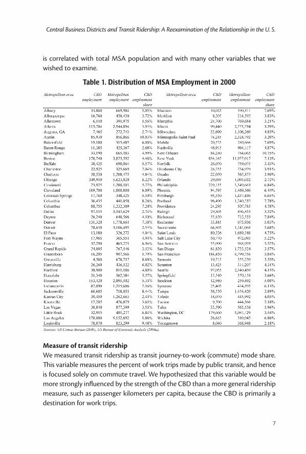
Measure of Urban Centralization versus DecentralizationOur urban structure variable is the share of MSA employment in the CBD for each MSA (CBD employment divided by total metropolitan employment). Table 1 lists CBD employment, total metropolitan employment, and CBD employment share (by MSA) in 2000. In 2000, Greenville, South Carolina, had the weakest CBD (0.68 percent of MSA employment), while New Orleans, Louisiana, had the strongest CBD (10.75 percent of MSA employment). The median MSA had 4.86 percent of its MSA employment inside its CBD in 2000.
We selected employment, as opposed to population, as our measure of centraliza-tion versus decentralization for three reasons. First, employment decentralization is the focus of most of the literature on urban decentralization and transit ridership that we discussed earlier in the paper. Second, recent studies have found a closer connection between transit ridership and employment than between ridership and population (Brown and Thompson 2008b). Third, employment tends to be collocated with most other travel destinations, which is why it is used as a proxy for these other destinations in most travel demand models used by transporta-tion planners. We decided to express CBD employment as a percent variable, as opposed to number of jobs in CBD, because CBD size (expressed in count form)
7
Central Business Districts and Transit Ridership: A Reexamination of the Relationship in the U. S.
is correlated with total MSA population and with many other variables that we wished to examine.
Table 1. Distribution of MSA Employment in 2000
Measure of transit ridershipWe measured transit ridership as transit journey-to-work (commute) mode share. This variable measures the percent of work trips made by public transit, and hence is focused solely on commute travel. We hypothesized that this variable would be more strongly influenced by the strength of the CBD than a more general ridership measure, such as passenger kilometers per capita, because the CBD is primarily a destination for work trips.
Journal of Public Transportation, Vol. 15, No. 4, 2012
8
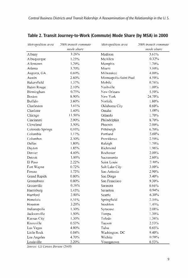
Table 2 reports the 2000 values for transit journey-to-work (commute) mode share by MSA. The smallest reported value for 2000 is found for McAllen, Texas (0.32 percent), while New York has the highest reported value (24.7 percent). The median MSA had a transit commute mode share of 1.98 percent in 2000.
We found significant differences in transit commute mode share among MSAs in our four population size groups. The median value for MSAs in the very large MSA group (population over 10 million, 14.7% mode share) is 60 percent higher than the corresponding value for the large MSA group (population from 5 million to 10 million, 8.8% mode share). The median values for our smaller population groups are much lower than these values. The median value for our medium MSAs (population 1 million to 5 million, 2.4% mode share) is nearly twice as large as that for the small MSA group (population from 500,000 to 1 million, 1.2% mode share). These differences reinforced our decision to stratify the MSAs by group size for our multivariate analysis.
HypothesesThe literature suggests that transit ridership is tied to a metropolitan area’s urban structure and, in particular, to the strength of the CBD as a locus of economic activity. The purpose of this paper is to test this hypothesis, while also controlling for other internal and external factors that are hypothesized to influence transit ridership. We include the following variables in each of our models:
1. Percent of MSA employment in the CBD. This variable is our CBD strength variable and can be used to measure the degree of employment centralization or decentralization in the MSA. Based on the literature, we would expect to find a positive relationship between the percent of MSA employment in the CBD and transit ridership.
2. Fare per passenger kilometer (adjusted to 2005 dollars). This is a variable that is at least partially under the control of transit agency managers. We expect that MSAs where transit agencies have higher fares will have lower ridership.
3. Service frequency (ratio of vehicle kilometers to route kilometers). This is a variable that is at least partially under the control of transit agency manag-ers. We expect that MSAs where transit agencies offer more frequent service will have higher ridership.
4. Service coverage (ratio of route kilometers to population). This is a variable that is at least partially under the control of transit agency managers. We
9
Central Business Districts and Transit Ridership: A Reexamination of the Relationship in the U. S.
Table 2. Transit Journey-to-Work (Commute) Mode Share (by MSA) in 2000
Journal of Public Transportation, Vol. 15, No. 4, 2012
10
expect that MSAs where transit agencies offer more service coverage will have higher ridership.
5. Percent of MSA households that do not own an automobile. This is an external variable (i.e., not under the control of agency managers) that may influence transit ridership. Based on the literature discussed earlier, we expect that MSAs that have higher percentage of carless households will have higher levels of transit ridership.
6. MSA unemployment rate. This is an external variable that may influence transit ridership. We expect that MSAs with higher unemployment rates will have lower ridership, because riders would have less need to use transit to reach jobs.
7. Fuel price index. This is an external variable that may influence transit ridership. We use this variable as a general proxy for the cost of using an automobile. We expect that MSAs with high fuel prices will have high transit ridership.
Model SpecificationWe estimated three cross-sectional multivariate ordinary least squares regression models to test our hypotheses. We estimate separate models for all MSAs, medium MSAs, and small MSAs. Through comparison with the medium MSA and small MSA models, we can treat the all MSA model as a pseudo-model for the very large and large MSAs.
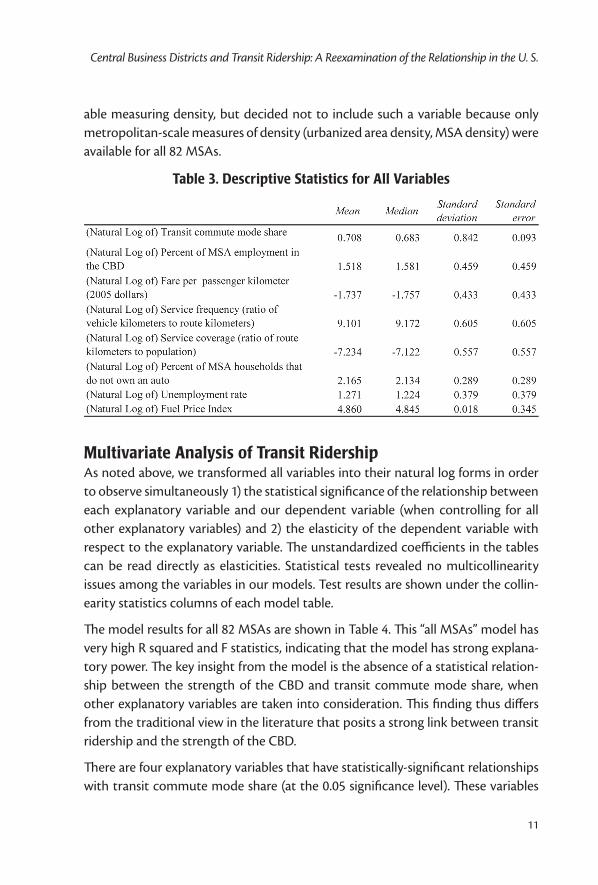
In evaluating the explanatory variables in each of the models, we are interested in the presence (or lack thereof) of statistical relationships and the practical importance of the statistical association. To measure practical importance, we use elasticity. In order to obtain elasticities, we transformed all the variables into their natural log forms. After this transformation, the coefficients for each explanatory variable can be read as the elasticity of the transit ridership variable with respect to the explanatory variable. We report descriptive statistics for our transformed variables in Table 3.
We tested the use of MSA population as a control variable, but decided not to include it because it was not statistically significant in any of our preliminary mod-els. Our MSA stratification appears to have accounted for the variation in transit ridership (by population size group) discussed earlier in the paper. We also tested the percent of MSA population made up of recent immigrants in our preliminary tests but decided not to include it because it was not correlated with our transit ridership variables. We suspect this is due to the wide dispersion of immigrant populations throughout the United States. We considered the inclusion of a vari-
11
Central Business Districts and Transit Ridership: A Reexamination of the Relationship in the U. S.
able measuring density, but decided not to include such a variable because only metropolitan-scale measures of density (urbanized area density, MSA density) were available for all 82 MSAs.
Table 3. Descriptive Statistics for All Variables
Multivariate Analysis of Transit RidershipAs noted above, we transformed all variables into their natural log forms in order to observe simultaneously 1) the statistical significance of the relationship between each explanatory variable and our dependent variable (when controlling for all other explanatory variables) and 2) the elasticity of the dependent variable with respect to the explanatory variable. The unstandardized coefficients in the tables can be read directly as elasticities. Statistical tests revealed no multicollinearity issues among the variables in our models. Test results are shown under the collin-earity statistics columns of each model table.
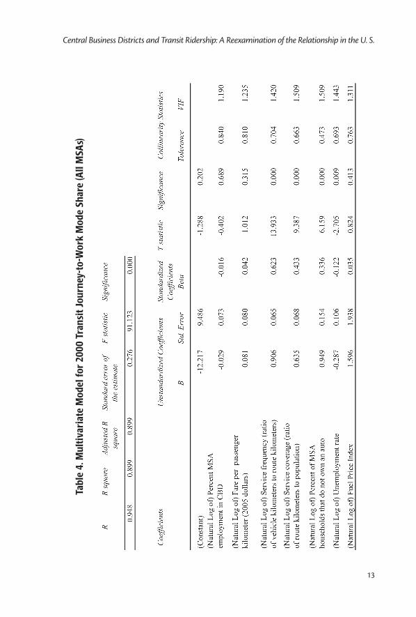
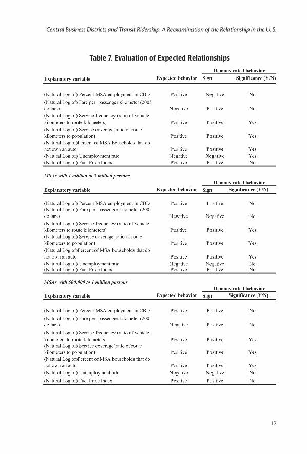
The model results for all 82 MSAs are shown in Table 4. This “all MSAs” model has very high R squared and F statistics, indicating that the model has strong explana-tory power. The key insight from the model is the absence of a statistical relation-ship between the strength of the CBD and transit commute mode share, when other explanatory variables are taken into consideration. This finding thus differs from the traditional view in the literature that posits a strong link between transit ridership and the strength of the CBD.
There are four explanatory variables that have statistically-significant relationships with transit commute mode share (at the 0.05 significance level). These variables
Journal of Public Transportation, Vol. 15, No. 4, 2012
12
are service frequency, service coverage, percent of MSA households that do not own cars, and unemployment rate. All four variables behaved as hypothesized. Two variables (service frequency and coverage) are under the control of transit man-agers. As service frequency and coverage increase, so does the transit commute mode share. The elasticities indicate that service frequency has a stronger effect on commute mode share than service coverage (elasticities of 0.906 and 0.635, respectively). This finding is consistent with other literature.
The other two variables are beyond the control of transit managers. Perhaps not surprisingly, the larger the share of carless households in the MSA, the higher the transit commute mode share. In fact, this variable has the strongest effect on tran-sit commute mode share (elasticity of 0.949). In addition, and also not surprisingly, the economic health of the metropolitan area has an effect on the transit commute mode share. As unemployment rates increase, transit commute mode share falls.
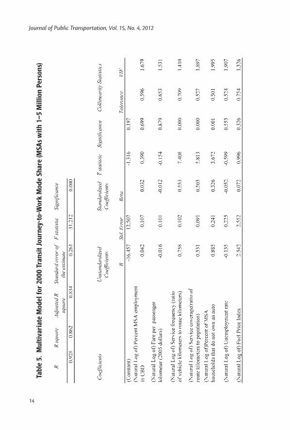
The second model, shown in Table 5, focuses on the relationship between transit commute mode share and our set of explanatory variables in the medium sized MSAs (population of 1 million to 5 million). The model has high R squared and F statistics, indicating that it is a strong explanatory model. As with our first model, we found no statistical relationship between the strength of the CBD and transit ridership.
Three of the four explanatory variables that were significant in the first model are also significant in this model. These variables are: service frequency, service coverage, and the percent carless households. All three variables behaved as hypothesized. As in the first model, MSAs whose transit agencies offered more frequent service and/or better service coverage had higher transit commute mode shares. As in the first model, MSAs with a higher percent of carless households had higher transit commute mode shares. These variables are inelastic with respect to transit commute mode share, with a similar rank order pattern as the model for all MSAs.
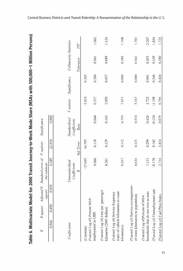
The third model, shown in Table 6, focuses on the relationship between transit commute mode share and our set of explanatory variables in the small MSAs (pop-ulation 500,000 to 1,000,000). Again, the R squared and F statistics indicate that this is a powerful model. This is the only one of the three models where our multi-collinearity test statistics are not comfortably within widely acceptable ranges. One variable, percent of MSA households that do not own a car, has collinearity sta-tistics that are just barely beyond this range, although the statistics are negligible.
13
Central Business Districts and Transit Ridership: A Reexamination of the Relationship in the U. S.
Tabl
e 4.
Mul
tiva
riat
e M
odel
for
2000
Tra
nsit
Jou
rney
-to-
Wor
k M
ode
Shar
e (A
ll M
SAs)
Journal of Public Transportation, Vol. 15, No. 4, 2012
14
Tabl
e 5.
Mul
tiva
riat
e M
odel
for
2000
Tra
nsit
Jou
rney
-to-
Wor
k M
ode
Shar
e (M
SAs
wit
h 1–
5 M
illio
n Pe
rson
s)
15
Central Business Districts and Transit Ridership: A Reexamination of the Relationship in the U. S.
Tabl
e 6.
Mul
tiva
riat
e M
odel
for
2000
Tra
nsit
Jou
rney
-to-
Wor
k M
ode
Shar
e (M
SAs
wit
h 50
0,00
0–1
Mill
ion
Pers
ons)
Journal of Public Transportation, Vol. 15, No. 4, 2012
16
The results of the small MSA model are very similar to the results for the other two models. As before, we found no statistically significant association between strength of the CBD and transit commute mode share, when other explanatory variables are taken into account. As with the other models, the service frequency, service coverage and percent carless household variables are significant and behave as expected. As with the other models, service frequency is more important than ridership (elasticities of 0.857 and 0.634, respectively), although the percent car-less household variable is the most important of the three explanatory variables (elasticity of 1.113).
In summary, the three models show that CBD strength is not associated with tran-sit commute mode share. This finding runs counter to our initial hypotheses (see Table 7). However, all the statistically significant relationships are consistent with our initial hypotheses.
DiscussionOur multivariate analysis indicates that transit commute mode share is not tied to the strength of the CBD when we take into account the other important influ-ences on transit ridership discussed by the literature. The lack of any meaningful statistical connection between the strength of the CBD and transit commute mode share is at odds with some of the literature cited earlier, but this disconnect can be explained. First, the literature cited earlier that reflects the traditional view either defines the strength of the CBD differently (as, for example, the absolute number of jobs in the CBD) or relies on very simple models that do not control for other variables that the authors themselves recognize can influence transit rider-ship. Second, our results are consistent with an emerging body of literature, best exemplified by Brown and Thompson (2008b), which examines the link between transit patronage and the distribution of employment in more nuanced ways. They distinguished between 1) employment inside the CBD, 2) employment outside the CBD but inside the transit service area, and 3) employment outside the transit service area. They found a strong link between the latter two types of employment and transit ridership (positive with respect to the second type of employment and negative with respect to the third type of employment). We were unable to obtain a variable equivalent to their measure of MSA employment outside the CBD but inside the transit service area. It is likely that if we had been able to do so, our results would have echoed their findings.
17
Central Business Districts and Transit Ridership: A Reexamination of the Relationship in the U. S.
Table 7. Evaluation of Expected Relationships
Journal of Public Transportation, Vol. 15, No. 4, 2012
18
Transit commute mode share is, however, tied to several other variables, some of which are (at least partially) within the control of transit managers. Higher transit ridership is strongly associated with higher service frequency and is also associ-ated, albeit slightly less strongly, with better service coverage. Our analysis suggests that agencies will be rewarded with higher ridership if they improve their service frequency or their coverage. However, the likely effects of these policy decisions on service productivity cannot be inferred from this analysis. Of course, it is possible that the key service variables (route miles and service frequency) have larger values where ridership is higher, which raises the possibility that they are endogenous variables. However, the consistency of these statistical results with other work, par-ticularly in the service orientation and service productivity literature, suggests that this might not be the case and that riders are indeed responding to agency deci-sions to provide better service in more locations (Brown and Thompson 2008c). Transit ridership is also tied to factors beyond the control of transit agency manag-ers, including the percent of carless households in the MSA. Unemployment rates are also important, as indicators of overall regional economic health, in particular MSA settings.
Based on our finding that transit commute mode share is not tied to CBD strength, there is the suggestion that transit managers have adjusted their service strategies to better serve decentralized urban environments. However, further research is required to identify the specific strategies they have employed and to determine the effectiveness of these strategies.
References
Beesley, M., and M. Kemp. 1987. Urban transportation. In Mills, E. (ed.), Handbook of Regional and Urban Economics, Volume II: Urban Economics. North Holland Press, Amsterdam.
Brown, J., and G. Thompson. 2008a. Examining the influence of multi-destination service orientation on transit service productivity: A multivariate analysis. Transportation 35(2): 237–252.
Brown, J., and G. Thompson. 2008b. The relationship between transit ridership and urban decentralization: Insights from Atlanta. Urban Studies 45(5&6): 1119–1139.
19
Central Business Districts and Transit Ridership: A Reexamination of the Relationship in the U. S.
Brown, J., and G. Thompson. 2008c. Service orientation, bus-rail service integra-tion, and transit performance: An examination of 45 U.S. metropolitan areas. Transportation Research Record 2042: 82–89.
Ferreri, M. 1992. Comparative costs. In Gray, G. E., and L. A. Hoel (eds.), Public Trans-portation, Second Edition. Prentice-Hall, Englewood Cliffs, NJ.
Florida Department of Transportation. 2005. Florida Transit Information System 2005. Available for download at lctr.eng.fiu.edu/ftis/.
Gómez-Ibáñez, J. 1996. Big city transit ridership, deficits and politics: Avoiding real-ity in Boston. Journal of the American Planning Association 62(1): 30–50.
Hartgen, D., and M. Kinnamon. 1999. Comparative Performance of Major U.S. Bus Transit Systems, 1988–1997. Sixth Edition. Charlotte, NC: Center for Interdisci-plinary Transportation Studies, University of North Carolina at Charlotte.
Heilbrun, J. 1987. Urban Economics and Public Policy, Third Edition. St. Martin’s Press, New York.
Hendrickson, C. 1986. A note on trends in transit commuting in the United States relating to employment in the central business district. Transportation Research Part A 20(1): 33–37.
Jones, D. 1985. Urban Transit Policy: An Economic and Political History. Prentice-Hall, Englewood Cliffs, New Jersey.
Kain, J. 1997. Cost-effective alternatives to Atlanta’s rail rapid transit system. Journal of Transport Economics and Policy January: 25–49.
Kain, J., and Z. Liu. 1999. Secrets of success: Assessing the large increases in transit ridership achieved by Houston and San Diego transit providers. Transportation Research Part A 33(7/8): 601–624.
Kitamura, R. 1989). A causal analysis of car ownership and transit use. Transporta-tion 16(2): 155–173.
Kohn, H. 2000. Factors affecting urban transit ridership. Paper presented at the Bridging the Gaps Conference, Charlottetown, PEI, Canadian Transportation Research Forum.
McCollom, B., and R. Pratt. 2004. Transit pricing and fares. In Traveler Response to Transportation System Changes, Report 95, Transit Cooperative Research
Journal of Public Transportation, Vol. 15, No. 4, 2012
20
Program, Transportation Research Board, National Research Council, Wash-ington, D.C.
McLeod, M., K. Flannelly, L. Flannelly, and R. Behnke. 1991. Multivariate time-series model of transit ridership based on historical, aggregate data: The past, pres-ent and future of Honolulu. Transportation Research Record 1297: 76–84.
Meyer, J., and J. Gómez-Ibáñez. 1981. Autos, Transit, and Cities. Harvard University Press, Cambridge, MA.
Meyer, J., J. Kain, and M. Wohl. 1965. The Urban Transportation Problem. Harvard University Press, Cambridge, MA.
Mierzejewski, E., and W. Ball. 1990. New findings on factors related to transit use. ITE Journal, February: 34–39.
Office of Management and Budget, Executive Office of the President. 2005. Update of statistical area definitions and guidance on their uses. OMB Bulletin 06-01, dated December 5.
Pisarski, A. 1996. Commuting in America II. Eno Foundation, Washington, D.C.
Pucher, J. 2002. Renaissance for public transport in the United States. Transporta-tion Quarterly 56 (1): 33–49.
Pucher, J., and J. Renne. 2003. Socioeconomics of urban travel: Evidence from the 2001 NHTS. Transportation Quarterly 57 (3): 49–78.
Pushkarev, B., and J. Zupan. 1977. Public Transportation and Land Use Policy. Indiana University Press, Bloomington, IN.
Pushkarev, B., and J. Zupan. 1980. Urban Rail in America. Indiana University Press, Bloomington, IN.
Stanley, R., and R. Hyman. 2005. Evaluation of recent ridership increases. Research Results Digest 69, Transit Cooperative Research Program, Transportation Research Board, National Research Council, Washington, D.C.
Taylor, B. 1991. Unjust equity: An examination of California’s transportation devel-opment act. Transportation Research Record 1297: 85–92.
Taylor, B., and D. Miller. 2003. Analyzing the determinants of transit ridership using a two-stage least squares regression on a national sample of urbanized areas. Paper presented at the 82nd Annual Meeting of the Transportation Research Board, Washington, D.C.
21
Central Business Districts and Transit Ridership: A Reexamination of the Relationship in the U. S.
Thompson, G. and Brown, J. 2006. Explaining variation in transit ridership in U.S. metropolitan areas between 1990 and 2000: A multivariate analysis. Transpor-tation Research Record 1986: 172–181.
Thompson, G., and T. Matoff. 2003. Keeping up with the Joneses: Planning for transit in decentralizing regions. Journal of the American Planning Association 69(3): 296–312.
TRL Limited. 2004. The Demand for Public Transport: A Practical Guide. TRL Report TRL 593.
U.S. Bureau of Economic Analysis (2006a). Employment (by County). Available at http://www.bea.gov/bea/regional/reis/defaultcfm?&catable=CA25&series=SIC.
U.S. Bureau of Economic Analysis. 2006b. Population (by county). Available at http://www.bea.gov/bea/regional/reis/default.cfm?catable=CA1-3.
U.S. Bureau of Labor Statistics. 2005a. 2000 Tabulation of unemployment rates from the current population survey. Available at http://www.bls.gov/cps, accessed July 1, 2005.
U.S. Bureau of Labor Statistics. 2005b. Consumer Price Index. Available at http://www.bls.gov, accessed July 1, 2005.
U.S. Bureau of Labor Statistics. 2005c. Consumer Price Index: Motor fuel. Available at http://www.bls.gov, accessed July 1, 2005.
U.S. Census Bureau. 1982. Census of retail trade. Government Printing Office: Washington, D.C.
U.S. Census Bureau. 2000. Census Transportation Planning Package. Bureau of Transportation Statistics, Washington, DC.
About the Authors
Jeffrey R. Brown ([email protected]) is Associate Professor and Director of the Master’s Program in the Department of Urban and Regional Planning at Florida State University. His research interests include the early professionalization of transporta-tion planning, the changing nature of street and highway planning in the United States, transportation finance, and the relevance of different service strategies for making public transit more successful in decentralized urban areas.
Journal of Public Transportation, Vol. 15, No. 4, 2012
22
Dristi Neog ([email protected]) is an Assistant Professor at the Sushant School of Art and Architecture, Gurgaon, India, and a Fellow of the Sus-tainable Planet Institute, Gurgaon, India. She is anchoring a Master’s program in Sustainable Urbanism at the Sushant School and her research interests include sustainable transportation planning and analysis, transportation and land use dynamics, sustainable development, transit planning and application of geographic information systems (GIS) to sustainable urban planning.
Planning Public Transport Networks—The Neglected Influence of Topography
23
Planning Public Transport Networks—The Neglected Influence
of TopographyRhonda Daniels
Corinne Mulley, The University of Sydney
Abstract
The principles of public transport network planning include coverage, frequency, legibility and directness. But trade-offs are made in implementing these principles, reflecting the economic, institutional, temporal, and natural environments in which public transport is planned, funded, and operated. Analysis of the case study of Syd-ney, Australia, shows how implementing network planning principles is influenced by the natural environment. The neglected influence of topography on public trans-port network planning can be improved through understanding of the impact of topography on planning, expansion, operations, and public transport use; measur-ing the nature of the walk access in providing coverage; ensuring planning guidelines recognize topography in measuring walking access; and choosing the most efficient mode topographically while ensuring other policies support multimodal networks.
IntroductionThe impact of the physical environment on urban form is well-known, as is the relationship between urban form and transport use. But the role of the physical environment in influencing the provision of public transport has been neglected, with the principles of public transport network planning often overturned by topography. The paper concentrates on the role of topography in the spatial aspects of network planning decisions including coverage, frequency, legibility, and
Journal of Public Transportation, Vol. 15, No. 4, 2012
24
directness. The paper identifies and discusses how topography is a factor in many aspects of public transport, from network planning, network growth, operations, and use. Sydney, with its physical geography of coastal location, harbors, bays, riv-ers, and deeply dissected plateaus, is used as a case study to analyze how topogra-phy influences rail, bus, and ferry and the elements of public transport planning, growth, operations and use.
The paper is structured as follows: First, network planning principles are discussed. Then the impact of topography on public transport planning, network expansion, operations and use are identified, followed by a case study of Sydney that discusses the impact of topography on public transport in Sydney. The last section discusses and identifies how to better recognize the impact of topography in public trans-port network planning.
Network Planning PrinciplesPublic transport networks reflect interactions among the economic, institutional, temporal, and physical environments in which they have developed and currently exist. The economic environment includes the budget available for public trans-port and cost constraints for capital investment, operations and maintenance (Colin Buchanan and Partners 2003). Institutional environments determine the governance and regulatory environment of who plans, funds, provides, and regu-lates public transport (Van de Velde 1999). The temporal environment includes his-torical factors and the legacy of previous decisions on transport and land use and the modes of public transport available, which is why the network design at any one point in time is a function of its historical evolution (Barker and Robbins 1963). The physical environment includes elements of the natural environment such as climate and topographical features, including water features of harbors, bays and rivers and land features of peninsulas, ridges, slopes, and elevations.
Theoretical guidance on planning spatial networks, from a customer-oriented per-spective as opposed to the operational determination of network design, is scarce. HiTrans Best Practice Guide for medium-size European cities is a recent guide for practitioners that fills the gap, noting that “by tradition, public transport opera-tions have been a practical, non-academic business” (Neilsen et al. 2005, p. 14). Nielsen et al. (2005, p. 168) also note that a literature review did not reveal sources of comprehensive network planning advice. In the U.S., a single chapter (Pratt and Evans 2004) provides guidance on bus routing and coverage in the U.S. While there is no commonly-cited set of principles for planning public transport networks,
Planning Public Transport Networks—The Neglected Influence of Topography
25
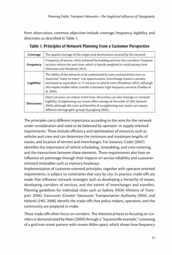
from observation, common objectives include coverage, frequency, legibility, and directness as described in Table 1.
Table 1. Principles of Network Planning from a Customer Perspective
Coverage The spatial coverage of the origins and destinations covered by the network.
FrequencyFrequency of service, often achieved by building services into corridors. Frequent services reduce the wait time, which is heavily weighted in total journey time (Abrantes and Wardman 2011).
Legibility
The ability of the network to be understood by users and potential users to maximize “many to many” trip opportunities. Interchange creates a penalty estimated as equivalent to 17 minutes in-vehicle time (Wardman 2001), although this maybe smaller when transfer is between high-frequency services (Paulley et al. 2006).
Directness
Direct services can reduce travel time. Directness can also impinge on network legibility. Straightening out routes offers savings of the order of 30% (Jansson 2003), although the costs and benefits of straightening out routes can impact different demographic groups (Ljungberg 2005).
The principles carry different importance according to the aims for the network under consideration and need to be balanced by operator- or supply-oriented requirements. These include efficiency and optimization of resources such as vehicles and crew and can determine the minimum and maximum lengths of routes, and location of termini and interchanges. For instance, Ceder (2007) identifies the importance of vehicle scheduling, timetabling, and crew rostering and the interactions between these elements. These requirements also have an influence on patronage through their impacts on service reliability and customer-oriented timetables such as memory headways.Implementation of customer-oriented principles, together with operator-oriented requirements, is subject to constraints that vary by city. In practice, trade-offs are made that influence network strategies such as developing a hierarchy of routes, developing corridors of services, and the extent of interchanges and transfers. Planning guidelines for individual cities such as Sydney (NSW Ministry of Trans-port 2006), Vancouver (Greater Vancouver Transportation Authority 2004), and Helsinki (HKL 2008) identify the trade-offs that policy makers, operators, and the community are prepared to make.
These trade-offs often focus on corridors. The theoretical basis to focusing on cor-ridors is demonstrated by Mees (2000) through a “Squaresville example,” consisting of a grid-iron street pattern with streets 800m apart, which shows how frequency
Journal of Public Transportation, Vol. 15, No. 4, 2012
26
can be enhanced with a given set of resources. However, this assumes services are planned on a featureless, flat plain and does not recognize land use and urban form. High-frequency corridors create a network effect that, with interchange, can expand the number of different destinations that passengers can access at good levels of frequency. While this is a good planning principle, HiTrans (Neilsen et al. 2005, p. 89) recognizes that in practice, two different types of restrictions for the exploitation of the network effect are common: low demand insufficient to sup-port high-frequency services, and infrastructure capacity restrictions both for rail and road-based modes of public transport.
The economic environment is becoming more important, with today’s public transport provision increasingly facing budget constraints. Trade-offs that concen-trate services in corridors, thus enhancing frequency, are seen as good strategies to increase patronage (Currie and Wallis 2008). Pratt and Evans (2004) suggest for the U.S. that planning should simplify and straighten routes so as to provide for new travel demand patterns and remove interchange. In contrast, HiTrans (Neilsen et al. 2005) promotes the focus on simple, high-frequency networks based on high-frequency corridors that provide the network effect for an urban area by relying on transfers and interchanges between routes and modes. This latter approach could be seen as the “European” approach, in which integrated ticketing with no penalty for transfer has been a longstanding feature, well before the introduction of electronic ticketing.
This section on network planning principles has concentrated on the bus mode. In planning multimodal networks, rail-based routes are regarded as fixed in loca-tion, with flexibility achieved by the addition of bus-based services to develop a network. The fixity of rail services means that their contribution to spatial changes in network design is limited, and network planning and design for rail corridors considers only elements such as timing, frequency, and interchange opportunities.
Influence of Topography on Public Transport Planning PrinciplesThe network planning principles of coverage, frequency, legibility, and directness assume a featureless plain. In practice, network planning principles are heavily constrained by the natural environment and topography in both the initial devel-opment and growth of a network. Topography has affected both the historical development of modes and public transport networks as well as the restructur-ing of current networks and expansion and growth of networks. Moreover, the
Planning Public Transport Networks—The Neglected Influence of Topography
27
influence of topography on public transport operations and public transport use is often underestimated in development of public transport networks. Topogra-phy can influence all modes of public transport through its impacts on planning, network expansion, operations, and public transport use. These factors are clearly inter-related and can have a cumulative influence.
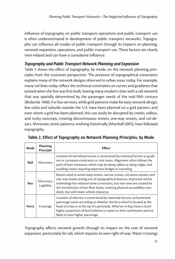
Topography and Public Transport Network Planning and ExpansionTable 2 shows the effect of topography, by mode, on the network planning prin-ciples from the customer perspective. The presence of topographical constraints explains many of the network designs observed in urban areas today. For example, many rail lines today reflect the technical constraints on curves and gradients that existed when the line was first built, leaving many modern cities with a rail network that was spatially determined by the passenger needs of the mid-19th century (Bedarida 1968). For bus services, while grid patterns make for easy network design, few cities and suburbs outside the U.S. have been planned on a grid pattern, and even where a grid has been planned, this can easily be disrupted by creeks, valleys, and rocky outcrops, creating discontinuous streets, one-way streets, and cul-de-sacs. Moreover, street patterns, evolving historically (Marshall 2005), have followed topography.
Table 2. Effect of Topography on Network Planning Principles, by Mode
ModePlanning Principle
Effect
Rail Directness
Location of rail infrastructure is constrained by technical factors or gradi-ent or curvature constraints or cost issues. Alignment often follows the path of least resistance, which may be along valleys or along ridges, and avoiding routes requiring expensive bridges or tunneling
BusDirectness, Legibility
Routes need to avoid steep streets, narrow streets, circuitous streets, and one-way streets arising out of topographical features. Improved vehicle technology has reduced some constraints, but new ones are created by the introduction of low-floor buses, meeting physical accessibility stan-dards, but with lower vehicle clearance.
Ferry Coverage
Location of wharves is constrained by waterside factors, and potential patronage varies according to whether the ferry wharf is located at the head of a bay or at the tip of a peninsula. Wharves in bays have a much higher proportion of land (relative to water) in their catchments and are likely to have higher patronage.
Topography affects network growth through its impact on the cost of network expansion, particularly for rail, which requires its own right-of-way. Water crossings
Journal of Public Transportation, Vol. 15, No. 4, 2012
28
of rivers or harbors, whether by bridge or tunnel, can be expensive, as can tunneling to provide suitable gradients. Topography affects the nature of tunneling material, whether sandstone, silts, or sands, and therefore choice of alignments for new links and location of stations. This is clearly illustrated in the case study of Sydney below.
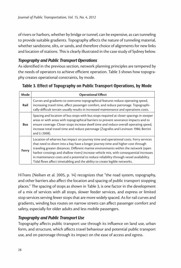
Topography and Public Transport OperationsAs identified in the previous section, network planning principles are tempered by the needs of operators to achieve efficient operation. Table 3 shows how topogra-phy creates operational constraints, by mode.
Table 3. Effect of Topography on Public Transport Operations, by Mode
Mode Operational Effect
RailCurves and gradients to overcome topographical features reduce operating speed, increasing travel time, affect passenger comfort, and reduce patronage. Topographi-cally-difficult terrain usually results in increased maintenance and operations costs.
Bus
Spacing and location of bus stops with bus stops required at closer spacings in steeper areas or with areas with topographical barriers to prevent severance impacts and to ensure coverage. Closer stops increase dwell time and reduce overall operating speed, increase total travel time and reduce patronage (Zografos and Levinson 1986; Bertini and Li 2008).
Ferry
Location of wharves has impact on journey time and operational costs. Ferry services that need to divert into a bay have a longer journey time and higher cost through traveling greater distances. Different marine environments within the network (open harbor crossings and shallow rivers) increase vehicle mix, with consequential increases in maintenance costs and a potential to reduce reliability through vessel availability. Tidal flows affect timetabling and the ability to create legible networks.
HiTrans (Neilsen et al. 2005, p. 14) recognizes that “the road system, topography, and other barriers also affect the location and spacing of public transport stopping places.” The spacing of stops as shown in Table 3, is one factor in the development of a mix of services with all stops, slower feeder services, and express or limited stop services serving fewer stops that are more widely spaced. As for rail curves and gradients, winding bus routes on narrow streets can affect passenger comfort and safety, especially for older adults and less mobile passengers.
Topography and Public Transport UseTopography affects public transport use through its influence on land use, urban form, and structure, which affects travel behaviour and potential public transport use, and on patronage through its impact on the ease of access and egress.
Planning Public Transport Networks—The Neglected Influence of Topography
29
Understanding of urban form and land use, including the size of centers, hierarchy of centers, and center location, is underpinned by the theory of land rent-gradients in a homogeneous physical environment, as summarized in Evans (1985). But topography disturbs these theoretical outcomes. Aspects of land use and urban form affected by topography include concentration of development along cor-ridors such as waterways or ridges, the location of centers, and the catchments for centers, including severance impacts of topographical barriers. Topography can influence the density of development through creating locations perceived to be attractive or unattractive. In the early days of urban development, steep slopes may initially have been considered unattractive due to construction difficulties and higher cost. Over time, land and steep slopes that offer water views have become more attractive and are now likely to have higher densities of development.
Related to this, the urban form and the built environment, influenced by the physical environment of topography, in turn influence travel behaviour including choice of mode (Cervero and Kockelman 1997; Cervero 2002; Handy et al. 2005). Quantifying the direct impact of the physical environment on public transport use is less well understood as it is limited by data and measurement complexities. For instance, Taylor et al. (2009) proposed a conceptual model of the factors influenc-ing aggregate transit demand, including regional geography, which includes popu-lation, density, and area as well as regional topography/climate. However, there were no data source for regional topography/climate.
For access and egress to public transport, there are data and measurement dif-ficulties, including self-selection, where reported studies capture those people who have made the decision to walk given the environment. Taking a different approach, Wibowo and Olszewski (2005) investigated the effort of walking to access public transport in Singapore and found the effort to climb one ascending step is equal to 2.8m of level walking, so the effort to climb one pedestrian bridge with 32 ascending steps is equal to 90m of walking.
Overall, the discussion on public transport planning, operations, and use sug-gests that the network planning principles identified previously may be seriously constrained by topography. Networks that are developed in cities with diverse topographical elements may well end up with a public transport network that looks very different from that suggested by the planning principles. The next sec-tion considers Sydney, the capital of New South Wales, Australia, as a case study to illustrate the constraints imposed by topography on public transport as well as some of the solutions that are transferable elsewhere in the world.
Journal of Public Transportation, Vol. 15, No. 4, 2012
30
Case Study: SydneySydney’s TopographyWhile all the state capital cities in Australia are founded on rivers and share some aspects of Sydney’s topography such as bays, harbors, and a coastal location, the combination of diverse topographical features in Sydney’s physical environment is unique. Sydney, the capital of New South Wales and Australia’s largest city, is a global city centered on a spectacular harbor and surrounded by national parks and ocean beaches (NSW Government 2005).
Sydney’s distinctive topography includes its coastal location, dominated by the drowned river valley forming Sydney Harbour based on the Parramatta and Lane Cove rivers. Other rivers flowing generally from the west east to the coast include the Georges River, Cooks River, and Hacking River to the south of the harbor, creat-ing Botany Bay and Port Hacking. The Hawkesbury–Nepean River is the western and northern boundary to Sydney, flowing at the base of the Blue Mountains to the west and entering the ocean to the north of the city. The rivers and their many creeks and tributaries dissect Sydney, creating ridges, plateaus and valleys. The many rivers also create peninsulas of development along the harbor, which are highly valued for their water views and amenity but can be difficult to serve efficiently by public transport. North of Sydney Harbour, Middle Harbour divides the Lower North Shore from the northern beaches. The northern beaches area has many coastal lagoons, and the long, narrow Pittwater peninsula is a distinctive landform in the far north.
Sydney’s colonial development was affected by this topography, with the first European settlement in 1788 at Sydney Cove on the eastern edge of the Sydney basin, on the southern side of the large harbor. Sydney’s land use strategy notes the impact of topography on development:
If the first fleet had settled at Parramatta rather than Circular Quay, Sydney would be a more typical global city, such as London and Paris, with the CBD in the middle of the urban area on relatively flat ground next to a river that could be bridged eas-ily. Sydney, however, grew from a town perched on the harbor at the eastern edge of the Sydney basin, then spread quickly to the more fertile areas south and west along the rivers, across the flatter lands to the west, and eventually north across the harbor (NSW Government 2005, p. 32).
In the growth of Sydney, land that was initially considered more difficult to build on or less suitable for agriculture, such as rocky outcrops or steep slopes, was left
Planning Public Transport Networks—The Neglected Influence of Topography
31
undeveloped and often preserved as parks and reserves. Indeed, “almost half of Sydney [comprises] national parks, State Forests, regional and local space, water catchments, and wetlands that are protected from inappropriate development” (NSW Government 2005, p. 204).
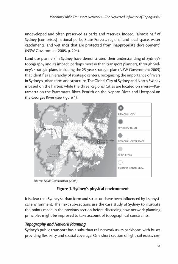
Land use planners in Sydney have demonstrated their understanding of Sydney’s topography and its impact, perhaps moreso than transport planners, through Syd-ney’s strategic plans, including the 25-year strategic plan (NSW Government 2005) that identifies a hierarchy of strategic centers, recognizing the importance of rivers in Sydney’s urban form and structure. The Global City of Sydney and North Sydney is based on the harbor, while the three Regional Cities are located on rivers—Par-ramatta on the Parramatta River, Penrith on the Nepean River, and Liverpool on the Georges River (see Figure 1).
Source: NSW Government (2005)
Figure 1. Sydney’s physical environment
It is clear that Sydney’s urban form and structure have been influenced by its physi-cal environment. The next sub-sections use the case study of Sydney to illustrate the points made in the previous section before discussing how network planning principles might be improved to take account of topographical constraints.
Topography and Network PlanningSydney’s public transport has a suburban rail network as its backbone, with buses providing flexibility and spatial coverage. One short section of light rail exists, cre-
Journal of Public Transportation, Vol. 15, No. 4, 2012
32
ated from the conversion of a previous freight corridor. An extensive ferry network provides connections across the harbor and mitigates, to a certain extent, the lack of water crossings. This section first considers the topographical constraints on the rail network, as this in itself provides knock-on issues for the other modes.
Sydney’s rail network reflects the technical constraints on curves and gradients that existed when lines were first built and that still affect network expansion. For instance, Sydney’s North Shore follows a tortuous route north of the harbor, reflecting technical constraints on grade and curvature when being built in the 1890s. As with many “river” cities, Sydney is constrained by limited water crossings, with only three in total over a river distance of 30km, the first being the iconic Harbour Bridge, completed in 1932.
Topography also has an influence on the network and route planning of Sydney bus services. Very few, if any, parts of Sydney have extensive suburbs with a grid street pattern. Even where subdivisions may have been planned on a traditional grid pattern, the implementation of the grid pattern on the ground is disrupted by creeks, valleys, and cliffs, leading to discontinuous streets, one-way streets, and cul-de-sacs. Few major bus corridors in Sydney are straight, direct routes and are predominantly routes first established many years ago. Many roads in early colo-nial Sydney were based on walking tracks along ridges used by Aboriginal people. These walking tracks developed into roads and, later, tram lines. When bus services replaced trams in the 1950s, they continued to serve the development that had built up around the tram lines. Major bus corridors with a concentration of services forming a radial network into the CBD twist and turn, following ridges. Even where land is flatter, such as the Cumberland Plain in western Sydney, the location of resi-dential and commercial development has been constrained by floodplains. In turn, this has affected the demand for public transport and, consequently, the design of bus routes as part of the network.
Ferries provide important links and, often, much faster access. The ferries not only provide cross-harbor links, providing extra capacity for the water crossing, but are also successful where journeys by bus would be very circuitous because of topogra-phy. For example, in southern Sydney, Bundeena is a small community on the south-ern shore of Port Hacking surrounded by national park. The privately-operated ferry service, which takes approximately 30 minutes between Bundeena and Cronulla, provides an important public transport link as an alternative to the 30-km, 45-min drive from Bundeena through the national park to the nearest station.
Planning Public Transport Networks—The Neglected Influence of Topography
33
Topography and Network Growth and ExpansionTopographical constraints had several related impacts on the most recent rail net-work expansion—the Epping-Chatswood Rail Line, which opened in 2009. There were two options for the proposed rail line to cross the Lane Cove River in the Lane Cove National Park: either a tunnel under the river to minimize visual amenity and vegetation impacts, or a high-level bridge across the river. The decision to cross the river in a tunnel meant that a proposed station at an isolated university campus (UTS Ku-ring-gai) to the east of the river was deleted because the station would be too deep. The gradients involved in rising from the tunnel under the river also meant a longer length of track was required to connect into the existing surface North Shore line. The longer track increased construction cost and increased travel time. In addition, some existing rolling stock could not use the new line due to the impact of steepness on power requirements.
Rail construction costs affected by topography affected decisions made over 2008–2010 on the cancellation of the heavy rail North West Rail Link and its replacement metro rail projects, the North West Metro and CBD Metro. The original concept for the North West Rail Link in flatter western Sydney included an elevated section of track to avoid floodplains. One of the attractions of metro rail as a replacement for the heavy rail North West Rail Link was the smaller tunnel size required and cheaper tunneling costs. Sydney is built on sandstone, which has a high cost for tunneling at up to $400 million per km (NSW Government 2009). While the prop-erties of Sydney sandstone are generally considered good for tunneling, unpredict-able fault lines can be encountered. As a replacement for the North West Rail Link, the North West Metro project was announced in March 2008, with 32 of 37 km in tunnel and 4 harbor crossings (Darling Harbour, White Bay at the Anzac Bridge, Iron Cove at the Iron Cove Bridge, and under the Parramatta River at the Glades-ville Bridge) at a total cost of $12 billion (escalated cost for completion in 2017). Due to the cost of the project and the state’s declining fiscal position, the North West Metro project was canceled in October 2008 and replaced by the shorter CBD Metro project. At 9 km and requiring only 2 harbor crossings, it cost $4.8 billion when announced, but increased to $5.3 billion 6 months later due to uncertainty. The CBD Metro itself was canceled in early 2010. This history illustrates the way in which extending or creating new links in an old and established network that is subject to topographical constraints can be very costly and difficult to justify on normal evaluation procedures.
Journal of Public Transportation, Vol. 15, No. 4, 2012
34
Topography and OperationsIn Sydney, topography affects public transport operating speeds, travel time and costs, and, thus, patronage. On the Sydney rail network, the four main corridors to access the metropolitan network are shared by passenger and freight services. Passenger services have priority on the metropolitan network, with freight services usually restricted from operating on lines in peak times. But due to the topography, it is difficult to provide separate space for dedicated lines for freight and passen-gers. Widening corridors requires blasting through sandstone cliffs and widening water crossings, which can be done, but at a cost.
On the Sydney Light Rail in inner Sydney, the route alignment and station locations were affected by the topography of the sandstone headland. The route uses the existing circuitous freight alignment that was originally carved through sandstone, with the result being slow travel times as well as very deep stations with low vis-ibility and poor access.
With bus services, topography affects operational issues such as the speed of buses and the location of bus stops. The major northern corridor of the Spit Bridge across Middle Harbour illustrates operational impacts, where the steep approaches on both sides of the bridge—with elevation of 95m on the south, 6m at the bridge and 70m on the north—and the winding access on the southern approach slows down buses. In addition, traffic stops while the bridge opens and shuts six times each weekday (in the off-peak) to allow boats in and out of Middle Harbour and eight times each weekend day.
In Sydney, ferries operate in three environments with different characteristics: across the heads of Sydney Harbour to Manly, in the inner harbor, and up the Par-ramatta River. The variety of operating environments requires a mix of vessels from ocean-rated vessels to vessels with low draught and low wash for upper river opera-tions. Walker (2007) discussed the negative impact of fleet diversity on reliability and cost and recommended reducing the number of vessel classes. In contrast to Sydney, Brisbane ferry services operate on the Brisbane River with a single class of vessel. In addition, because of local topography, some Sydney Harbour ferry wharves are accessible to passengers only by steep stairs.
Topography and Public Transport UseIn Sydney, both land use and urban structure as well as access to public transport are affected by topography. This section gives an example from each mode.
Planning Public Transport Networks—The Neglected Influence of Topography
35
Sutherland Shire in the south of the Sydney is bounded by water on three sides, with the ocean to the east, Georges River and Botany Bay to the north, and Port Hacking to the south. A tributary flowing into the Georges River further divides the Shire into east and west portions. There are limited river crossings connecting the area to the rest of the city to the north, with only one rail crossing across the Georges River.
Sutherland Shire is also characterized by a series of narrow peninsulas of residential development to the north and to the south, which are difficult to serve efficiently by bus. Sutherland Shire Council has created an accessibility index for individual parcels of land that includes topography through gradient (Koernicke 2007), show-ing how residents of these peninsulas, which are often very steep, have more lim-ited public transport and less provision of services than the ridge areas of the shire, showing a lower level of accessibility.
North of the harbor, the northern beaches region of is similarly isolated, with lim-ited access points across Middle Harbour and limited rail access. Ferries provide an important link between Manly on the north shore and the CBD.
DiscussionNetwork Planning in SydneyWhile topography has clearly influenced Sydney’s public transport, it is more dif-ficult to determine whether topographical constraints have helped or hindered Sydney’s public transport development and use. Sydney has developed into Aus-tralia’s largest city, with the highest public transport mode share of any Australian city both for the journey to work and for all trip purposes (BITRE 2009). With a CBD-focused rail network, more than 70 percent of work trips to the Sydney CBD are by public transport (Transport Data Centre 2008). In addition to its CBD, Syd-ney has a strong set of suburban centers, identified in the Metropolitan Strategy as Regional Cities and Major Centres. But have these suburban centers developed in response to poor or good public transport? The 3 Regional Cities and 9 of the 11 Major Centres are served by rail and connected by a network of Strategic Bus Corridors, but less well so than the CBD. Public transport use for work trips to the non-CBD centres varies from 10 percent to just over 40 percent (TDC 2008). Park-ing is still readily available at most non-CBD centres.
The topographical constraints identified previously have been posited as being all “bad” for public transport network planning, operations, and use. However, these same topographical barriers can serve to channel demand into more concentrated
Journal of Public Transportation, Vol. 15, No. 4, 2012
36
services. As such, the constraints may make some services viable where this might not have otherwise been the case. But concentrating services into constrained corridors can also lead to bottlenecks that create adverse congested conditions, particularly if there is competition between public transport and the private car. To effectively concentrate patronage using the topographical constraints positively requires government to identify public transport as the key or only user of the corridor.
Network planning in Sydney is guided by the Service Planning Guidelines: Sydney Contract Regions (NSW Ministry of Transport 2006). While network planning focuses on connecting centers, guidelines are unhelpful in not using the same lan-guage to identify the hierarchy of centers as the strategic land use plan. In Sydney, bus networks are planned as a hierarchy of routes: Regional Routes, District Routes, and Local Routes. Criteria in the guidelines include:
• Coverage:Ninetypercentofhouseholds tobewithin400mofa rail lineand/or a Regional or District bus route during commuter peaks, interpeak and weekend day time; and 90 percent of households to be within 800m of a rail line and/or a Regional or District bus route at other times.
• Network legibility:Peakandoff-peakservicesshouldusethesameroutewherever possible.
• Routedesign(directness):Maximumdiversionfromthefastestorshortestroute (between termini) to be no more than 20 percent.
The network area coverage criterion is the key benchmark, calculated “as the crow flies.” As this paper has demonstrated, 400m of steep access is very different from access of 400m along flat land. It is clear that the guidelines treat Sydney as uni-form, with no allowance for different physical environments. In addition, by aiming to provide the same spatial coverage to everyone, it does not take account of the way in which topographically-difficult areas may require a disproportionate alloca-tion of the public transport budget for both capital and operating costs. In turn, this raises equity issues since in Sydney, as with other waterside cities, people with higher incomes live in the more attractive and expensive locations, such as water-fronts, which are the more challenging and expensive to serve by public transport.
Implications for Public Transport Network Planning While any city has a unique combination of features, and Sydney is no excep-tion, there are more general lessons that can be learned from the case study for implementing and understanding trade-offs among the four planning principles of
Planning Public Transport Networks—The Neglected Influence of Topography
37
coverage, frequency, legibility, and directness in the presence of topographical con-straints. The implementation of these lessons will vary depending on the institu-tional and regulatory environment for public transport planning. The most impor-tant message is for a centralized regulatory environment in which the government provides planning guidelines; here, the planning guidelines should recognize the influence of topography in terms of coverage and the way this is related to access and egress from public transport stops and stations. In deregulated environments where operators plan services to maximize revenue or profit, they may give more primacy to corridor strategies at the expense of coverage.
For consumers, the case study shows topography has the most influence on strat-egies to achieve coverage of origins and destinations. Coverage of origins is often expressed as a walk distance to a bus stop, such as 400 m. Guidelines for Vancouver, Canada, for example, reduce the expected walking distance for steep grades (GVTA 2004). Perth guidelines (Public Transport Authority 2003) have a goal of a bus stop within 500m of 95 percent of Perth’s population but recognize the pedshed concept for walkable catchments, defined as actual area within a 400m (5-minute) walking distance, expressed as a percentage of the theoretical area within a 400m walking distance, where a good target is 60 percent. In network planning principles, coverage should be calculated by reference to walking accessibility in terms of the equivalent walk effort required, not just distance, as shown by Wibowo and Olsze-wski (2005).
While GIS can be used to take topography including gradients into account, fur-ther research is needed to better understand which elements of topography affect people’s walking decisions—Can footpaths overcome steep gradients? How much does gradient influence walking distance? Are more stops required in steeper areas?
As topography influences location of land uses and the transport that accesses land uses, transport and land use planners must encourage and support integrated transport and land use planning through strategic and local planning to ensure that major land uses and centers are located where they can be served efficiently by public transport.
ConclusionThe case study of Sydney, with its combination of topographical features, highlights the two-way process of the relevance of taking topography into account in the planning and provision of public transport and the way in which the development of public transport is influenced by topography. A failure to recognize the impact of

Journal of Public Transportation, Vol. 15, No. 4, 2012
38
topography in, for example, planning guidelines, can give regressive equity impacts from trade-offs among network planning principles of coverage, frequency, legibil-ity and directness. Moreover, the presence of topographical constraints means that extending the public transport system is expensive in both capital and operational terms, with trade-offs between the areas to serve becoming necessary in a budget-ary and evaluation constrained environment.
Topography would be better taken into account in public transport network planning in several ways: better understanding its impact on planning, expansion, operations, and public transport use; better measuring the nature of the walk access in providing coverage; ensuring that planning guidelines measure walking access realistically, recognizing topography; and choosing the most efficient mode topographically while ensuring that other policies support multimodal networks. Integrated transport and land use planning can also ensure that public transport is provided most efficiently in topographically-constrained environments.
References
Abrantes, P. A. L., and M. R. Wardman. 2011. Meta-analysis of UK values of travel time: An update. Transportation Research Part A 45(1): 1–17.
Barker, T. C., and M. Robbins. 1963. A History of London Transport, Vol. 1: The Nine-teenth Century. George Allen and Unwin.
Bedarida, F. 1968. The growth of urban history in France: Some methodological trends. In Dyos, H. J. (ed.), The Study of Urban History. London: Edward Arnold.
Bertini, R. L., and H. Li. 2008. Toward optimal transit stop spacing. Sixth Interna-tional Conference on Traffic & Transportation Studies (ICTTS), Nanning, China, August 5–8. http://web.pdx.edu/~bertini/papers/spacing_ICTTS2008_final.pdf.
BITRE. 2009. Information Sheet 31—Urban passenger transport: How people move about in Australian cities. Bureau of Infrastructure, Transport and Regional Economics, Canberra.
Ceder, A. 2007. Public Transit Planning and Operation. Oxford, UK: Butterworth Heinemann.
Planning Public Transport Networks—The Neglected Influence of Topography
39
Cervero, R. 2002. Built environments and mode choice: Toward a normative framework. Transportation Research Part D: Transport and Environment 7(4): 265–284.
Cervero, R., and K. Kockelman. 1997. Travel demand and the 3Ds: Density, diversity, and design. Transportation Research Part D: Transport and Environment 2(3): 199–219.
Colin Buchanan and Partners. 2003. Transferability of Best Practice in Trans-port Policy Delivery: Final Report. http://www.scotland.gov.uk/Publica-tions/2003/08/17895/23881.
Currie, G., and I. Wallis. 2008. Effective ways to grow urban bus markets: A synthesis of evidence. Journal of Transport Geography 16(6): 419–429.
Evans, A. W. (1985) Urban Economics, An Introduction. Oxford, UK: Basil Blackwell.
Greater Vancouver Transportation Authority. 2004. Transit Service Guidelines Pub-lic Summary Report, GVTA.
Handy, S., X. Cao, and P. Mokhtarian. 2005. Correlation or causality between the built environment and travel behaviour? Evidence from Northern California. Transportation Research Part D: Transport and Environment 10(6): 427–444.
HKL. 2008. Public Transport Planning Guidelines in Helsinki. HKL Publication Series A: 1/2008, HKL Planning Unit, Helsinki.
Jansson, J. O. 2003. Key factors for boosting the bus transport market in medium-size towns. Competition and Ownership in Land Passenger Transport Thredbo 8.
Koernicke, I. 2007. Accessibility constraints mapping for walking and public transport in the Sutherland Shire. Papers of the 30th Australasian Transport Research Forum, Melbourne. www.patrec.org/atrf.aspx
Ljungberg, A. 2005. Using Geographic Information System (GIS) doing CBA on new bus route systems—An empirical example of the city of Linkoping. 9th Confer-ence on Competition and Ownership in Land Transport, Lisbon, Portugal.
Marshall, S. 2005. Streets and Patterns. London: Spon Press.
Mees, P. 2000. A Very Public Solution. Melbourne.
Neilsen, G., J. D. Nelson, C. Mulley, G. Tegner, G. Lind, and T. Lange. 2005. HiTrans Best Practice Guide 2: Public Transport—Planning the Networks. HiTrans, www.hitrans.org.
Journal of Public Transportation, Vol. 15, No. 4, 2012
40
NSW Government. 2005. Metropolitan Strategy City of Cities: A Plan for Sydney’s Future. December, www.metrostrategy.nsw.gov.au.
NSW Government. 2009. Public Notice: Grants Distribution. The Sydney Morning Herald, 30 September.
NSW Ministry of Transport. 2006. Service Planning Guidelines: Sydney Contract Regions. June. www.transport.nsw.gov.au/busreform/service-planning-guide-lines.pdf.
Paulley, N., R. Balcombe, R. Mackett, H. Titheridge, J. Preston, M. Wardman, J. Shires, and P. White. 2006. The demand for public transport: The effects of fares, qual-ity of service, income and car ownership. Transport Policy 13(4): 295–306.
Pratt, R., and R. Evans. 2004. Bus routing and coverage. Chapter 10, Traveler Response to Transportation System Changes, TCRP 95. Transportation Research Board, Washington DC.
Public Transport Authority. 2003. Design and Planning Guidelines for Public Trans-port Infrastructure: Bus Route Planning and Transit Streets. Western Australia.
Taylor, B., D. Miller, H. Iseki, and C. Fink. 2009. Nature and/or nurture? Analyzing the determinants of transit ridership across U.S. urbanized areas. Transportation Research A: Policy and Practice 43A(1): 60–77.
Transport Infrastructure Development Corporation. 2008. North West Rail Link Supplementary Submissions Report. March, Sydney, http://majorprojects.plan-ning.nsw.gov.au/files/21028/Submissions%20Report%20Part%2001.pdf.
Transport Data Centre. 2008. Transfigures employment and commuting in Syd-ney’s centres, 1996–2006. Transport Data Centre, NSW Ministry of Transport, Sydney.
van de Velde, D. M. 1999. Organizational forms and entrepreneurship in public transport, Part 1: Classifying organizational forms. Transport Policy 6: 147–157.
Walker, B. 2007. Report of the special commission of inquiry into Sydney Ferries Corporation. October, www.transport.nsw.gov.au/inquiries/walker-ferry-report.pdf.
Wardman, M. 2001. A review of British evidence on time and service quality valua-tions. Transportation Research Part E 37: 107–128.
Planning Public Transport Networks—The Neglected Influence of Topography
41
Wibowo, S. S., and P. Olszewski. 2005. Modeling walking accessibility to public transport terminals. Case study of Singapore Mass Rapid Transit. Journal of the Eastern Asia Society for Transportation Studies 6: 147–156.
Zografos, K. G., and H. S. Levinson. 1986. Passenger service times for a non–fare bus system. Transportation Research Record 1051: 42–48.
About the Authors
Dr. Rhonda Daniels ([email protected]) was formerly a Senior Research Fellow in Public Transport at the Institute of Transport. She has public sector experience in transport planning, transport policy and integrating transport and land use in NSW and research interests in improving accessibility through public transport.
Professor Corinne Mulley ([email protected]) is the founding Chair in Public Transport at the Institute of Transport and Logistics Studies at the University of Sydney. As a transport economist, she has researched and published at the interface of transport policy and economics, in particular on issues relating to public transport. She led a high-profile European and UK consortia undertak-ing benchmarking in urban public transport and has provided both practical and strategic advice to local and national governments on benchmarking, rural trans-port issues, and public transport management. Prof. Mulley's research is motivated by a need to provide evidence for policy initiatives, and she has been involved in such research at local, regional, national, and European levels. She has an enduring interest in modern transport history and in the way it can inform current thinking about policy.

Journal of Public Transportation, Vol. 15, No. 4, 2012
42
43
The Effect of Proximity to Urban Rail on Housing Prices in Ottawa
The Effect of Proximity to Urban Rail on Housing Prices in OttawaChristopher M. Hewitt, M.A., and W. E. (Ted) Hewitt, Ph.D.
The University of Western Ontario
Abstract
Increasingly, urban rail transit (URT) is seen as a desirable solution for transporta-tion challenges faced by both urban planners and residents of suburban areas alike. The availability and ease of access to URT, in turn, may result in distortions in local real estate markets. The conventional wisdom, in fact, suggests that construction of urban rail lines serves as a magnet for new housing development and, in turn, can lead to increases in property values in proximity to URT stations. Existing studies have, in good measure, confirmed this belief, but largely on the basis of global area studies that can often mask locally differentiating factors affecting housing prices. Using data from the City of Ottawa, this study seeks to move beyond such analyses by using spatial regression and mapping techniques that reveal that the relationship between URT stations and housing prices is far more complex than is commonly believed. The study demonstrates that while at the macro-level housing prices do vary positively with proximity to URT stations, the relationship is spatially dependent and may be affected by factors unique to specific locales.
IntroductionUrban rail transit1 (URT) is an increasingly important feature in major cities insofar as it provides effective transportation to work, leisure activities, and shopping for citizens, particularly in suburban areas (Hess and Almeida 2007). There are also
1 Urban rail transit is any form of “rail [transit] in an urban area, including both heavy and light rail, which may be underground, at level or elevated” (Flyvbjerg 2007, 12).
Journal of Public Transportation, Vol. 15, No. 4, 2012
44
considerable cost savings accruing to transit users due to the reduced need for personal vehicles, as well as the satisfaction of knowing that one has contributed to positive environmental outcomes. As a consequence, there is often a desire to reside in proximity to URT stations, which provide easy access to the central busi-ness district (CBD) and other distant parts of the city.
To date, a number of studies have demonstrated a relationship between proximity to URT and property values (see, for example, Bowes and Ihlanfeldt 2001; Chen et al. 1998; Hess and Almeida 2007; Nelson and McCleskey 1990; Ryan 1999). For the most part, these have confirmed a conventional wisdom that suggests that residing near URT stations can have a positive impact on property values. In a limited num-ber of studies, however, the reverse has been shown; that is, living too close to URT lines may actually depress housing prices under certain circumstances, owing to inconveniences associated with construction and or operation of suburban trains (see, for example, Landis et al. 1995; Nelson 1992; Ryan 2005).
Using advanced spatial regression techniques in combination with detailed map-ping and employing a broad range of data from multiple sources, this study seeks to bring clarity to this debate by examining the effect of proximity to URT stations on property values in the city of Ottawa, Canada. In accord with virtually all studies on the topic to date, the study reveals URT location to, indeed, be a sound predic-tor of housing prices. It is also one, however, that is spatially defined and operates in a somewhat more complex fashion than the existing literature would suggest. Specifically, the research demonstrates that both positive and negative impacts of proximity to URT stations on housing prices are in evidence within the same sam-pling frame, largely dependent upon spatial location along URT lines.
Current Research on URT Location and Housing PricesFor this study, 22 analyses conducted between 1973 and 2010 focusing on the rela-tionship between URT location and housing prices were examined. The vast major-ity of studies were conducted in the United States, some involving multiple cities. About one-quarter were undertaken in other countries, primarily in Asia, with one each in Europe and Latin America. Only two academic studies examining the relationship between the two variables in the Canadian context—both conducted prior to 1985—were discovered, both focusing on the city of Toronto.
Overall, this body of research has presented somewhat divergent tendencies. For the most part, studies have shown a negative relationship between housing prices and distance to the location of URT stations. In other words, housing prices tend to

45
The Effect of Proximity to Urban Rail on Housing Prices in Ottawa
decline the farther away from the station the housing property is located. Studies conducted in Boston, Atlanta, Chicago, Portland, and Washington (Baum-Snow and Kahn 2000), Atlanta (Bowes and Inlanfeldt 2001; Nelson and McCleskey 1990), Buffalo (Hess and Almeida 2007), Dallas (Clower and Weinstein 2002), Philadelphia (Slater 1974), Portland (Al-Moasind et al. 1993; Dueker and Bianco 1999; Chen et al. 1998), San Diego (Duncan 2008), San Francisco (Weinberger 2001), Bangkok (Chalermpong 2007), Seoul (Bae et al. 2003), and Shanghai (Pan and Zhang 2008) all affirm this relationship at varying levels of strength. The two studies undertaken in Canada are similarly in accord. A study by Dewees (1976) found that site values increased within one-third mile of transit stations, while Bajic (1983) found that in an around the Spadina surface metro route, housing prices increased by approxi-mately $2,200, on average.
In other cases, however, findings have been less conclusive. In Landis et al.’s (1995) four-site examination of San Diego, San Francisco, Sacramento, and San Jose, the relationship between housing prices and distance to URT stations was both nega-tive and positive, suggesting that, in some cases, there is a definite downside to living near transit rail lines, possibly associated with noise pollution and visual esthetics. Similarly mixed results were reported by Nelson (1992) for Atlanta, Ryan (2005) for San Diego, and Munoz-Raskin (2010) for Bogotá.
To some extent, the methodologies employed by these studies may have precipi-tated this mixed outcome. For the most part using a hedonic model applied to the entire study area, the results almost invariably indicate a single rate of change for property values at increasing distances from URT stations (see, for example, Dun-can 2008; Lewis-Workman and Brod 1997; Pan and Zhang 2008). The models thus assume a stationary relationship between the housing prices and other possible explanatory variables across the board. In fact, any number of factors in addition to URT location may affect housing prices differentially in varying locations (see Bae et al. 2003; Hess and Almeida 2007; Munoz-Raskin 2010). This, in turn, suggests that property values likely can and do vary from one station to another, and that the rate of change over distance may also vary accordingly—all pointing to the fact that any relationship that is non-stationary over space will not be modeled particu-larly well by a single parameter estimate and, indeed, this global estimate may be locally very misleading (see Fotheringham et al. 2002).
Some of the attendant challenges demonstrated by these more limited studies may have been abated had they used a mapping approach in their analyses. In fact, while many do present maps, these are used almost exclusively for reference purposes
Journal of Public Transportation, Vol. 15, No. 4, 2012
46
only (Hess and Almeida 2007; Munoz-Raskin 2010; Pan and Zhang 2008; Zhang et al. 1998).2 For the most part, presentation of results is restricted to charts and graphs. While helpful, given the possibilities for relationship variance cited above, they sim-ply cannot visualize a spatial relationship effectively enough to catch these.
The primary contribution of this case study to the literature is to bring advanced multiple regression and spatial techniques to a more sophisticated level of under-standing of the relationship between housing prices and URT station locations. What it reveals, beyond the basic understanding of the relationship posited within the literature, is that conclusions based on global trends within regions often obscure different, and sometimes opposing, tendencies within defined localities. In revealing these hidden patterns, the study thus provides not only a methodology for future study of this issue, but tools of potential interest and use to urban planners.
Data and MethodologyThe research undertaken for this study was conducted in Ottawa, Canada, located on the south bank of the Ottawa River. Ottawa is Canada’s capital city, with a large government employment sector and in the heart of a metropolitan region with a population of approximately 1,000,000. The City’s URT line—known as the O-Train—was officially launched in 2001 (Sebree 2002). Currently, the O-Train runs along an eight-kilometer section of track originally constructed by the Canadian Pacific Railway for freight use (Transport Canada 2008). The line extends between the Bayview and Greenboro districts of the city, passing through industrial areas, shopping districts, and more densely-populated neighbourhoods (Transport Canada 2008). The O-Train and URT, in general, have also been subject to a series of studies undertaken by Transport Canada (2008) and the City of Ottawa (Abouhe-nidy 2008; Leclair 2002; Leclair 2004; City of Ottawa 2010; City of Ottawa et al. 2008) regarding feasibility and future potential.
A large number of sources were used in carrying out the research for this study. The reference data were collected from several sources. The road and rail network information was obtained from the 2003 Ottawa Topographic Mapping dataset maintained by the Serge A. Sauer Map Library at the University of Western Ontario (Ottawa 2003). The land use features were obtained from a secure website data-base that is distributed through the University’s library system (Western 2010). Key points of interest in the city were determined from the results of an O-Train survey
2 The review found that maps were used more frequently as reference maps to present the study area.
47
The Effect of Proximity to Urban Rail on Housing Prices in Ottawa
conducted in 2002 (Leclair 2002).3 Population change and public transit-related population attributes, defined at the census tract (2,500–8,000 inhabitants) and dissemination area (400–700 inhabitants) level, were obtained from Statistics Canada (Statistics Canada 2006a, 2006b, 2008). Reference information from these various sources was plotted using a geographic information system (GIS) devel-oped for the purpose of this study.
Data related to the primary variables under consideration were obtained from two sources. The O-Train route was obtained from the City of Ottawa website (City of Ottawa 2010) as well as reports prepared by the City of Ottawa (see McCormick Rankin Corp. and Delcan 2008). The exact locations of the O-Train stations were identified on Google Maps and then plotted on maps developed for this study. Distance datasets were calculated using GIS-based measurements of the distance (in meters) from each property by street route to the nearest O-Train station. Straight-line distance measurements to several significant “neighborhood” features including water bodies, park land, and the points of interest that were defined pre-viously were included as well.
The property dataset was obtained through written permission from the Ottawa Real Estate Board (REB) (Ottawa Real Estate Board 2010). Housing sales data were collected from specific neighborhoods within the study area, defined as those neighborhoods located within approximately four kilometers of the O-Train route. All sales were recorded for the calendar years 2006 to 2009, coinciding with census data collection and during a period well into the operational phase of the O-Train. Of the more than 80,000 properties populating the study area, the sold properties were examined (n=3735), which were then plotted as individual points on a map using the address mapping feature of ArcMap (Statistics Canada 2006a, 2008). Some duplicate data were present, owing to the fact that a number of properties had been sold more than once. For these properties, the simple mean selling price was calculated and the most recent selling date for that property was recorded. Along with property values, a number of specific residential attributes were also obtained from the Ottawa REB dataset. This included information on the style (apartment, single-detached, townhouse, etc.) and type (bungalow, two-story, split-level)4 of single-family dwellings under study and specific features such as number of garages, fireplaces, and so forth that may reasonably affect housing prices.
3 The interest points were South Keys Mall, Preston Street, Downtown, the University of Ottawa, and Carleton University. These are indicated on Figure 1.
4 Dwelling size and type were coded ordinally based on the average value of each category.

Journal of Public Transportation, Vol. 15, No. 4, 2012
48
An annotated list of all variables generated from the data referenced above is pre-sented in Table 1. A map of the Ottawa O-Train network is presented in Figure 1, and study points (properties) analyzed as part of this study are presented in Figure 2.
Table 1. Study Variables
Variable Type Variable Definition Units Source
Dependent VariablePRICE
Amount property sold for
$ OREB
Independent Variables
Proximity to O-Train Station
TOTAL_LENGWalking distance to
O-Train stationm
Calculated using Network Analyst
Property Variables BEDRS_TOT Number of bedrooms Count OREB
BATHS_TOT Number of bathrooms Count OREB
AREA_2 Area of property Ft2 OREB
TYPEVALUE Type of house Value OREB
STYLEVALUE Style of house Value OREB
BASEMENTVALevel of development
in the basementValue OREB
XGARAGES Number of garages Count OREB
AGE Age of property YearOREB (2010 –
year built)
FIREPLACE Number of fireplaces Count OREB
TOTAL_PA Amount of parking Count OREB
GROSS_TAX Amount of tax $ OREB
Location VariablesDist_WATR
Distance to nearest water feature
mCalculated as a
straight line
Dist_PARKDistance to nearest
parkm
Calculated as a straight line
Dist_POIDistance to point of in-terest as identified by O-Train user survey
mCalculated as a
straight line
Neighborhood Variables Pop_Change
Change in population from 1996 – 2001 and
2001 – 2006Count
Calculated from Census data
AVG_INC Average income $ Census data
PUBLIC_TRA Public transit users Count Census data
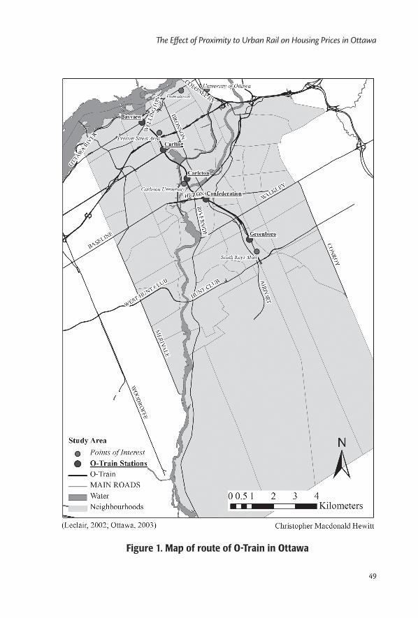
49
The Effect of Proximity to Urban Rail on Housing Prices in Ottawa
Figure 1. Map of route of O-Train in Ottawa
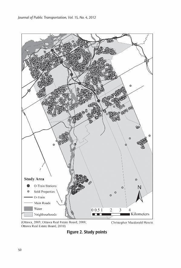
Journal of Public Transportation, Vol. 15, No. 4, 2012
50
Figure 2. Study points
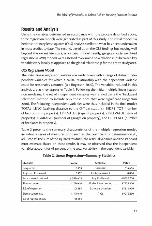
51
The Effect of Proximity to Urban Rail on Housing Prices in Ottawa
Results and AnalysisUsing the variables determined in accordance with the process described above, three regression models were generated as part of this study. The initial model is a hedonic ordinary least squares (OLS) analysis similar to what has been undertaken in most studies to date. The second, based upon the OLS findings but moving well beyond the extant literature, is a spatial model. Finally, geographically weighted regression (GWR) models were assessed to examine how relationships between key variables vary locally as opposed to the global relationship for the entire study area.
OLS Regression ModelThe initial linear regression analysis was undertaken with a range of distinct inde-pendent variables for which a causal relationship with the dependent variable could be reasonably assumed (see Rogerson 2010). The variables included in this analysis are as they appear in Table 1. Following the initial multiple linear regres-sion modeling, the set of independent variables was refined using the “backward selection” method to include only those ones that were significant (Rogerson 2010). The following independent variables were thus included in the final model: TOTAL_LENG (walking distance to the O-Train stations), BEDRS_TOT (number of bedrooms in property), TYPEVALUE (type of property), STYLEVALUE (style of property), XGARAGES (number of garages on property), and FIREPLACE (number of fireplaces in property).
Table 2 presents the summary characteristics of the multiple regression model, including a series of measures of fit such as the coefficient of determination R2, adjusted R2, the sum of the squared residuals, the residual variance, and the standard error estimate. Based on these results, it may be observed that the independent variables account for 45 percent of the total variability in the dependent variable.
Table 2. Linear Regression—Summary Statistics
Statistic Value Statistic Value
R-squared 0.453 F-statistic 514.464
Adjusted R-squared 0.452 Prob(F-statistic) 0.000
Sum squared residual 4.398e+13 Log likelihood -48630.700
Sigma-square 1.179e+10 Akaike info criterion 97275.300
S.E. of regression 108585 Schwarz criterion 97318.900
Sigma-square ML 1.177e+10 AICc 97275.430
S.E of regression ML 108484
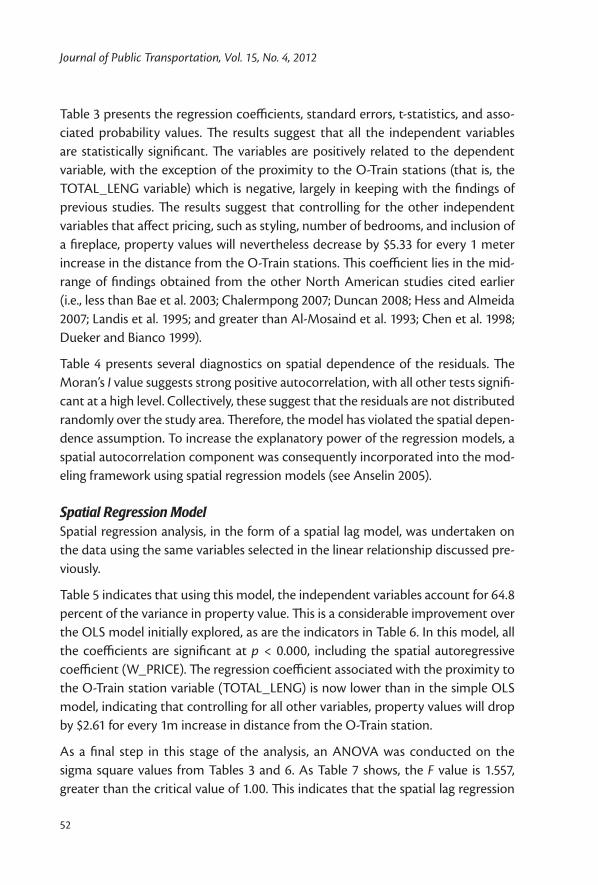
Journal of Public Transportation, Vol. 15, No. 4, 2012
52
Table 3 presents the regression coefficients, standard errors, t-statistics, and asso-ciated probability values. The results suggest that all the independent variables are statistically significant. The variables are positively related to the dependent variable, with the exception of the proximity to the O-Train stations (that is, the TOTAL_LENG variable) which is negative, largely in keeping with the findings of previous studies. The results suggest that controlling for the other independent variables that affect pricing, such as styling, number of bedrooms, and inclusion of a fireplace, property values will nevertheless decrease by $5.33 for every 1 meter increase in the distance from the O-Train stations. This coefficient lies in the mid-range of findings obtained from the other North American studies cited earlier (i.e., less than Bae et al. 2003; Chalermpong 2007; Duncan 2008; Hess and Almeida 2007; Landis et al. 1995; and greater than Al-Mosaind et al. 1993; Chen et al. 1998; Dueker and Bianco 1999).
Table 4 presents several diagnostics on spatial dependence of the residuals. The Moran’s I value suggests strong positive autocorrelation, with all other tests signifi-cant at a high level. Collectively, these suggest that the residuals are not distributed randomly over the study area. Therefore, the model has violated the spatial depen-dence assumption. To increase the explanatory power of the regression models, a spatial autocorrelation component was consequently incorporated into the mod-eling framework using spatial regression models (see Anselin 2005).
Spatial Regression ModelSpatial regression analysis, in the form of a spatial lag model, was undertaken on the data using the same variables selected in the linear relationship discussed pre-viously.
Table 5 indicates that using this model, the independent variables account for 64.8 percent of the variance in property value. This is a considerable improvement over the OLS model initially explored, as are the indicators in Table 6. In this model, all the coefficients are significant at p < 0.000, including the spatial autoregressive coefficient (W_PRICE). The regression coefficient associated with the proximity to the O-Train station variable (TOTAL_LENG) is now lower than in the simple OLS model, indicating that controlling for all other variables, property values will drop by $2.61 for every 1m increase in distance from the O-Train station.
As a final step in this stage of the analysis, an ANOVA was conducted on the sigma square values from Tables 3 and 6. As Table 7 shows, the F value is 1.557, greater than the critical value of 1.00. This indicates that the spatial lag regression
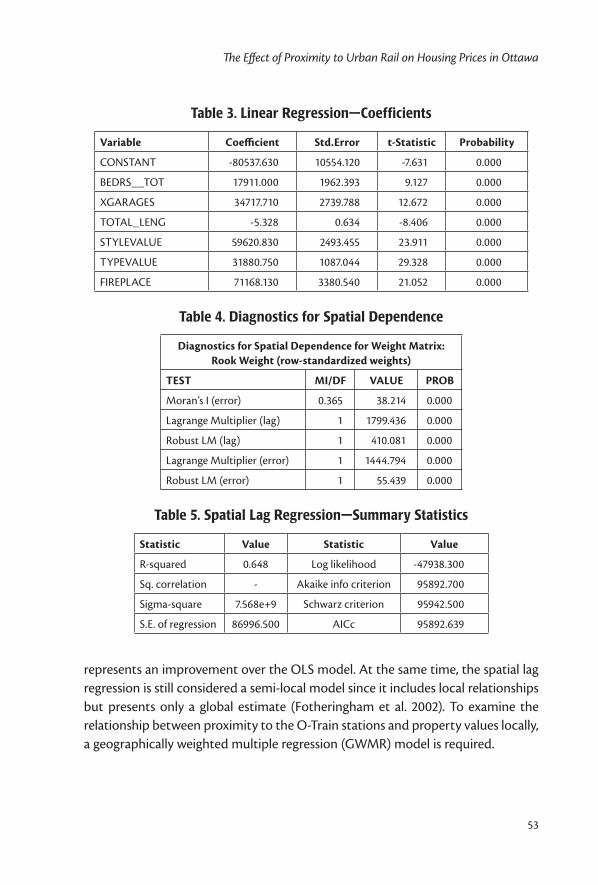
53
The Effect of Proximity to Urban Rail on Housing Prices in Ottawa
represents an improvement over the OLS model. At the same time, the spatial lag regression is still considered a semi-local model since it includes local relationships but presents only a global estimate (Fotheringham et al. 2002). To examine the relationship between proximity to the O-Train stations and property values locally, a geographically weighted multiple regression (GWMR) model is required.
Table 3. Linear Regression—Coefficients
Variable Coefficient Std.Error t-Statistic Probability
CONSTANT -80537.630 10554.120 -7.631 0.000
BEDRS__TOT 17911.000 1962.393 9.127 0.000
XGARAGES 34717.710 2739.788 12.672 0.000
TOTAL_LENG -5.328 0.634 -8.406 0.000
STYLEVALUE 59620.830 2493.455 23.911 0.000
TYPEVALUE 31880.750 1087.044 29.328 0.000
FIREPLACE 71168.130 3380.540 21.052 0.000
Table 4. Diagnostics for Spatial Dependence
Diagnostics for Spatial Dependence for Weight Matrix: Rook Weight (row-standardized weights)
TEST MI/DF VALUE PROB
Moran’s I (error) 0.365 38.214 0.000
Lagrange Multiplier (lag) 1 1799.436 0.000
Robust LM (lag) 1 410.081 0.000
Lagrange Multiplier (error) 1 1444.794 0.000
Robust LM (error) 1 55.439 0.000
Table 5. Spatial Lag Regression—Summary Statistics
Statistic Value Statistic Value
R-squared 0.648 Log likelihood -47938.300
Sq. correlation - Akaike info criterion 95892.700
Sigma-square 7.568e+9 Schwarz criterion 95942.500
S.E. of regression 86996.500 AICc 95892.639
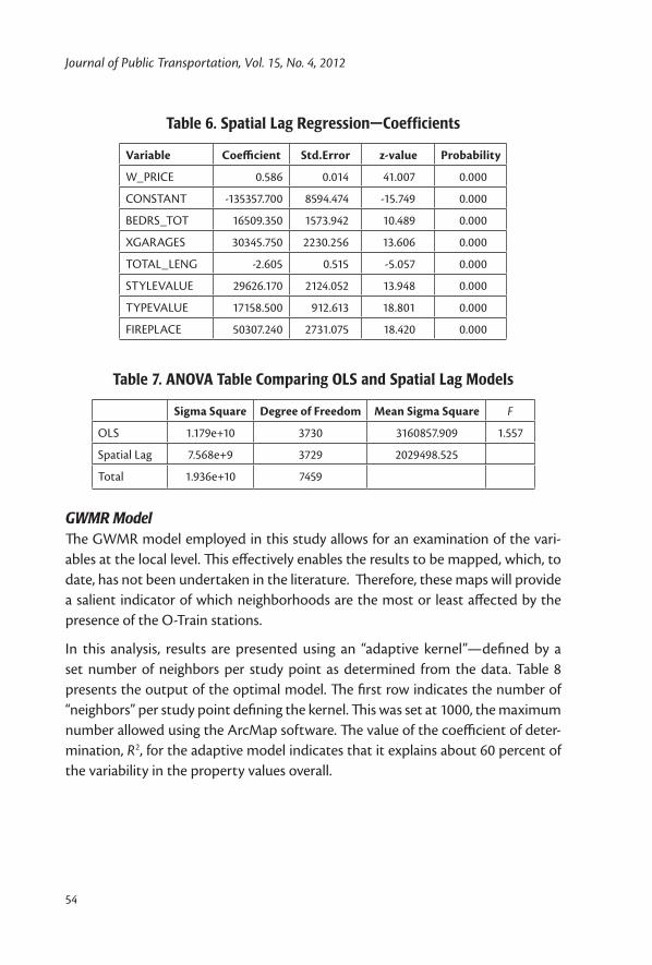
Journal of Public Transportation, Vol. 15, No. 4, 2012
54
Table 6. Spatial Lag Regression—Coefficients
Variable Coefficient Std.Error z-value Probability
W_PRICE 0.586 0.014 41.007 0.000
CONSTANT -135357.700 8594.474 -15.749 0.000
BEDRS_TOT 16509.350 1573.942 10.489 0.000
XGARAGES 30345.750 2230.256 13.606 0.000
TOTAL_LENG -2.605 0.515 -5.057 0.000
STYLEVALUE 29626.170 2124.052 13.948 0.000
TYPEVALUE 17158.500 912.613 18.801 0.000
FIREPLACE 50307.240 2731.075 18.420 0.000
Table 7. ANOVA Table Comparing OLS and Spatial Lag Models
Sigma Square Degree of Freedom Mean Sigma Square F
OLS 1.179e+10 3730 3160857.909 1.557
Spatial Lag 7.568e+9 3729 2029498.525
Total 1.936e+10 7459
GWMR ModelThe GWMR model employed in this study allows for an examination of the vari-ables at the local level. This effectively enables the results to be mapped, which, to date, has not been undertaken in the literature. Therefore, these maps will provide a salient indicator of which neighborhoods are the most or least affected by the presence of the O-Train stations.
In this analysis, results are presented using an “adaptive kernel”—defined by a set number of neighbors per study point as determined from the data. Table 8 presents the output of the optimal model. The first row indicates the number of “neighbors” per study point defining the kernel. This was set at 1000, the maximum number allowed using the ArcMap software. The value of the coefficient of deter-mination, R2, for the adaptive model indicates that it explains about 60 percent of the variability in the property values overall.
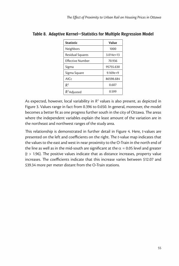
55
The Effect of Proximity to Urban Rail on Housing Prices in Ottawa
Table 8. Adaptive Kernel—Statistics for Multiple Regression Model
Statistic Value
Neighbors 1000
Residual Squares 3.014e+13
Effective Number 70.936
Sigma 95755.630
Sigma Square 9.169e+9
AICc 86598.684
R2 0.607
R2Adjusted 0.599
As expected, however, local variability in R2 values is also present, as depicted in Figure 3. Values range in fact from 0.396 to 0.650. In general, moreover, the model becomes a better fit as one progress further south in the city of Ottawa. The areas where the independent variables explain the least amount of the variation are in the northeast and northwest ranges of the study area.
This relationship is demonstrated in further detail in Figure 4. Here, t-values are presented on the left and coefficients on the right. The t-value map indicates that the values to the east and west in near proximity to the O-Train in the north end of the line as well as in the mid-south are significant at the α = 0.05 level and greater (t > 1.96). The positive values indicate that as distance increases, property value increases. The coefficients indicate that this increase varies between $12.07 and $39.34 more per meter distant from the O-Train stations.
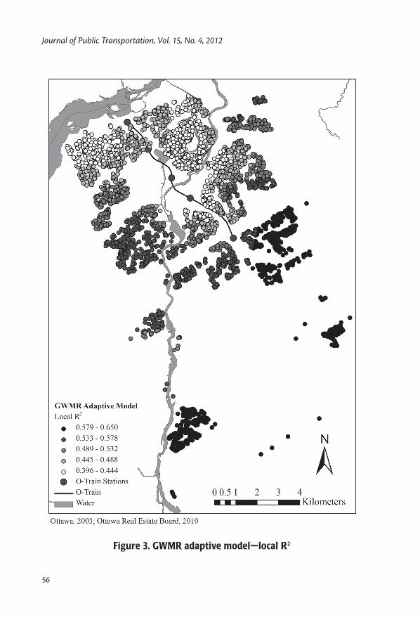
Journal of Public Transportation, Vol. 15, No. 4, 2012
56
Figure 3. GWMR adaptive model—local R2
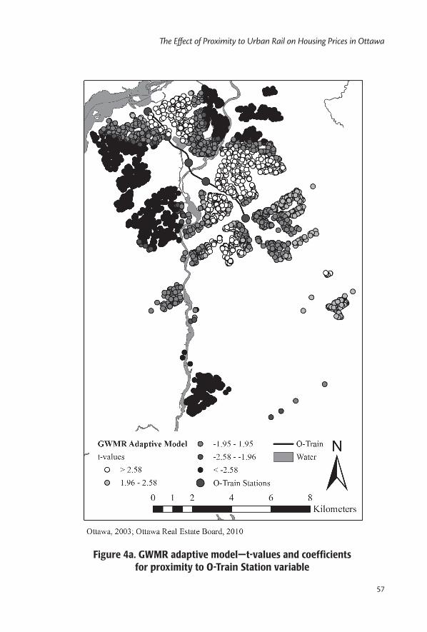
57
The Effect of Proximity to Urban Rail on Housing Prices in Ottawa
Figure 4a. GWMR adaptive model—t-values and coefficients for proximity to O-Train Station variable

Journal of Public Transportation, Vol. 15, No. 4, 2012
58
Figure 4b. GWMR adaptive model—t-values and coefficients for proximity to O-Train Station variable
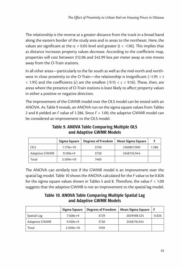
59
The Effect of Proximity to Urban Rail on Housing Prices in Ottawa
The relationship is the reverse at a greater distance from the track in a broad band along the eastern border of the study area and in areas to the northeast. Here, the values are significant at the α = 0.05 level and greater (t < -1.96). This implies that as distance increases property values decrease. According to the coefficient map, properties will cost between $12.06 and $42.99 less per meter away as one moves away from the O-Train stations.
In all other areas—particularly to the far south as well as the mid-north and north-west in close proximity to the O-Train—the relationship is insignificant (–1.95 < t < 1.95) and the coefficients (c) are the smallest (-9.15 < c < 9.16). These, then, are areas where the presence of O-Train stations is least likely to affect property values in either a positive or negative direction.
The improvement of the GWMR model over the OLS model can be tested with an ANOVA. As Table 9 reveals, an ANOVA run on the sigma square values from Tables 2 and 8 yielded an F value of 1.286. Since F > 1.00, the adaptive GWMR model can be considered an improvement to the OLS model.
Table 9. ANOVA Table Comparing Multiple OLS and Adaptive GWMR Models
Sigma Square Degrees of Freedom Mean Sigma Square F
OLS 1.179e+10 3730 3160857.909 1.286
Adaptive GWMR 9.169e+9 3730 2458176.944
Total 3.509e+10 7460
The ANOVA can similarly test if the GWMR model is an improvement over the spatial lag model. Table 10 shows the ANOVA calculated for the F value to be 0.826 for the sigma square values shown in Tables 5 and 8. Therefore, the value F < 1.00 suggests that the adaptive GWMR is not an improvement to the spatial lag model.
Table 10. ANOVA Table Comparing Multiple Spatial Lag and Adaptive GWMR Models
Sigma Square Degrees of Freedom Mean Sigma Square F
Spatial Lag 7.568e+9 3729 2029498.525 0.826
Adaptive GWMR 9.169e+9 3730 2458176.944
Total 3.509e+10 7459
Journal of Public Transportation, Vol. 15, No. 4, 2012
60
ConclusionsThe vast majority of previous studies examining proximity to URT stations and property value employed an OLS approach, while very few studies considered a spatial model. In addition, they tended uniformly to report global relationships. None effectively used more advanced techniques such as geographically weighted multiple regression (GWMR) to examine the relationship between the residential property values and proximity to URT stations at the local level. In addition, very few studies displayed their results as maps.
Given those limitations of previous studies, the aim of this research was to provide a comprehensive analysis of the relationship between the property values and proximity to URT stations using a variety of regression models and GIS tools.
This study established that the results of the hedonic OLS model used here (and by implication, other OLS models employed previously in the literature) were insuffi-cient for drawing conclusions about the relationship between proximity to O-Train stations and property values in Ottawa. This insufficiency was due to the problem of spatial autocorrelation of the residuals from the regression model. To correct for this, further analysis determined that a spatial model would be a better tool for analyzing the relationship. However, while identifying the existence of likely spatial differences, the model was able to provide only a global analysis of the relationship between proximity to the O-Train stations and property values. Consequently, a GWMR model was applied to analyze more directly the relationship locally. The study demonstrated, in fact, that the spatial lag model was the “optimal” method for examining the relationship both locally and globally.
In terms of its overall findings, the study demonstrated that while not the most important factor in determining house prices, there is a statistically significant rela-tionship between proximity to the O-Train stations and property values in the City of Ottawa. The results of the global regression analyses also indicated—in keeping with a large number of studies within the extant literature—that the relationship is negative; that is, the property values tend to decrease with increasing distance from the O-Train stations.
More importantly, however, the study revealed that such elementary analysis effectively hides a more complex relationship between the two variables under study. Further analysis clearly demonstrated that this is a relationship that also varies spatially; that is, the strength and direction of the relationship is locationally dependent, with housing prices in some areas affected positively and in other areas
61
The Effect of Proximity to Urban Rail on Housing Prices in Ottawa
negatively by distance from the O-Train stations. Specifically, many neighborhoods in closest proximity to the O-Train route saw a negative impact on housing prices, while many areas located further away experienced a significant increase. This, in turn, tends to support the finding of a small minority of studies to date that have been drawn to similar conclusions, albeit with less sophisticated tools (see, for example, Landis et al. 1995; Nelson 1992; Munoz-Raskin 2010).
There are several explanations potentially accounting for this result. One possible factor—mentioned frequently in the literature—relates to noise pollution and potentially bus and car traffic associated with the operation of the O-Train line. It may simply be that housing in proximity to the line is less desirable as homeowners seek the refuge of quieter streets located further away from the line. An associ-ated concern may be related to the history and potential future of the O-Train service. Before 2001, the O-Train line was used for freight trains. In fact, the track is still considered a freight line since the Canadian Pacific Railway maintains owner-ship (Transport Canada 2008). Therefore, property values may remain depressed in proximity to the O-Train line due to the possibility of a failure of the O-Train venture and a perceived eventual return to freight train travel through the cor-ridor. Properties of the surrounding area affecting affluence and or desirability of neighborhoods may also have an influence, such as distance from industrial parks, the CBD, parks, malls, and airports. Examination of all of these myriad influences remains, however, beyond the scope of this study. Further research may help to clarify the precise nature of these relationship variables and their correlation with the two primary variables.
Based upon this study, however, one outcome is clear—controlling for the myriad of factors that help determine property values, proximity to URT stations does have an impact on pricing, but one that varies depending on residential location. Along with its contribution to knowledge in this field, at very least, then, such infor-mation may be relevant and beneficial to future urban development in Ottawa and other regions where urban rail transit already exists or is planned. For urban planners, the study suggests the following cautions:
1. Depending upon the neighborhood, location of URT stations may not posi-tively affect property values and, thus, not be uniformly welcomed by local homeowners (or local-level political representatives).
2. Desirability of residing close to URTs and, thus, volume of usage of transit systems may not be uniform throughout the system.
3. Zoning in proximity to URT stations needs to take into account local features
Journal of Public Transportation, Vol. 15, No. 4, 2012
62
as well as factors associated with access to transit to take full advantage of land rents.
Acknowledgments
The authors would like to thank Carol Mallett for her assistance in providing access to the Ottawa real estate database and Dr. Jacek Malczewski for advice provided during both the data collection and analysis phases of this study.
References
Abouhenidy, M. 2008. Moving forward with rapid transit. White Paper, 34–40.
Al–Mosaind, M. A., K. J. Dueker, and J. G. Strathman. 1993. Light rail transit sta-tions and property values: A hedonic price approach. Transportation Research Record 1400: 90–94.
Anselin, L. 2005. Exploring spatial data with GeoDaTM: A workbook. Center for Spa-tially Integrated Social Science, Urbana, Illinois.
Bae, C.-H. C., M.-J. Jun, and H. Park. 2003. The impact of Seoul’s Subway Line 5 on residential property values. Transport Policy 10: 85–94.
Bajic, V. 1983. The effects of a new subway line on housing prices in Metropolitan Toronto. Urban Studies 20: 147–158.
Baum–Snow, N. and M. E. Kahn. 2000. The effects of new public projects to expand urban rail transit. Journal of Public Economics 77: 241–263.
Bowes, D. R., and K. R. Ihlanfeldt. 2001. Identifying the impacts of rail transit sta-tions on residential property values. Journal of Urban Economics 50: 1–25.
Chalermpong, S. 2007. Rail transit and residential land use in developing countries: Hedonic study of residential property prices in Bangkok, Thailand. Transporta-tion Research Record 2038: 111–119.
City of Ottawa, McCormick Rankin Corp., and Delcan. 2008. Transportation master plan infrastructure requirement study: Development of a downtown transit solution and network implications. Retrieved February 11, 2010, from www.ottawa.ca.
63
The Effect of Proximity to Urban Rail on Housing Prices in Ottawa
City of Ottawa. 2010, Last Update. City of Ottawa [Homepage for City of Ottawa, Canada]. Retrieved July 21, 2010, from www.ottawa.ca.
Clower, T. L., and B. L. Weinstein. 2002. The impact of Dallas Texas Area Rapid Transit light rail stations on taxable property valuations. Australasian Journal of Regional Studies 8(3): 389–400.
Dewees, D. 1976. The effect of a subway on residential property values in Toronto. Journal of Urban Economics 3: 357–369.
Dueker, K. J., and M. J. Bianco. 1999. Light rail transit impacts in Portland: The first ten years. Transportation Research Record 1685: 171–180.
Duncan, M. 2008. Comparing rail transit capitalization benefits for single-family and condominium units in San Diego, California. Transportation Research Record 2067: 120–130.
Flyvbjerg, B. 2007. Cost overruns and demand shortfalls in urban rail and other infrastructure. Transportation Planning and Technology 30: 1, 9–30.
Fotheringham, A. S., C. Brunsdon, and M. Charlton. 2002. Geographically Weighted Regression: The Analysis of Spatially Varying Relationships. Chichester: John Wiley & Sons, Ltd.
Hess, D. B., and T. M. Almeida. 2007. Impact of proximity to light rail rapid transit on station-area property values in Buffalo, New York. Urban Studies 44(5/6): 1041–1068.
Landis, J., S. Guhathukurta, W. Huang, M. Zhang, B. Fukuji, and S. Sen. 1995. Rail transit investments, real estate values, and land use change: A comparative analysis of five California rail transit systems. Research Report No. 48, Institute of Urban and Regional Studies, University of California, Berkeley.
Leclair, R. T. 2002. O–Train evaluation report. Retrieved October 26, 2010, from www.ottawa.ca.
Leclair, R. T. 2004. The O–Train: The straight facts. Retrieved October, 2010, from www.ottawa.ca.
Lewis-Workman, S., and D. Brod. 1997. Measuring the neighborhood benefits of rail transit accessibility. Transportation Research Record 1576: 147–153.
Munoz-Raskin, R. 2010. Walking accessibility to bus rapid transit: Does it affect property values? The Case of Bogota, Colombia. Transport Policy 17: 72–84.
Journal of Public Transportation, Vol. 15, No. 4, 2012
64
Nelson, A. C. 1992. Effects of elevated heavy rail transit stations on house prices with respect to neighborhood income. Transportation Research Record 1359: 127–132.
Nelson, A. C., and S. J. McCleskey. 1990. Improving the effects of elevated transit stations on neighborhoods. Transportation Research Record 1266: 173–180.
Ottawa. 2003. 1:10,000 scale topographic data. [computer file]. Ottawa: City of Ottawa.
Ottawa Real Estate Board. 2010. Last Update. MLXchange [Real Estate Website for Property Listings]. Retrieved June, 2010, from http://oreb.mlxchange.com/.
Pan, H., and M. Zhang. 2008. Rail transit impacts on land use: Evidence from Shang-hai, China. Transportation Research Record 2048: 16–25.
Rogerson, P. A. 2010. Statistical Methods for Geography. London: Sage Publications Ltd.
Ryan, S. 1999. Property values and transportation facilities: Finding the transporta-tion–land use connection. Journal of Planning Literature 13: 412–427.
Ryan, S. 2005. The value of access to highways and light rail transit: Evidence for industrial and office firms. Urban Studies 42(4): 751–764.
Sebree, G. M. 2002. O–Train: Is light rail on the verge of revolution? Trains 6211: 30–31.
Slater, P. B. 1973. Spatial and temporal effects in residential sales prices. Journal of the American Statistical Association 68343: 554–560.
Slater, P. B. 1974. Disaggregated spatial–temporal analysis of residential sales prices. Journal of the American Statistical Association 69346: 554–560.
Statistics Canada. 2006a. Census of population, 2006: Cartographic boundary, digi-tal boundary, ecumene, road network, road network and geographic attribute files/. Census of population, 2006: Maps [machine readable data file]. Ottawa, ON: Statistics Canada (producer), Statistics Canada, Data Liberation Initiative (distributors).
Statistics Canada. 2006b. Census of population, 2006: Geosuite: Population (2006/2001) and dwelling counts (2006) for census tracts [machine readable data file]. Ottawa, ON: Statistics Canada (producer), Statistics Canada, Data Liberation Initiative (distributors).
65
The Effect of Proximity to Urban Rail on Housing Prices in Ottawa
Statistics Canada. 2008. Census of population, 2006: Table 94–581–XCB2006002: Profile for Canada, provinces, territories, census divisions, census subdivisions and dissemination areas [machine readable data file]. Ottawa, ON: Statistics Canada (producer), Statistics Canada, Data Liberation Initiative (distributors).
Statistics Canada, 2010. 2006 Census Dictionary. Retrieved June, 10, 2010, from http://www12.statcan.gc.ca/census–recensement/2006/ref/dict/index–eng.cfm.
Transport Canada, 2008. O–Train light rail project. Case Studies in Sustainable Transportation, Case Study 7, 1–9.
Weinberger, R. R. 2001. Light rail proximity: Benefit or detriment in the case of Santa Clara County, California? Transportation Research Record 1747: 104–113.
Western. 2010. Equinox data delivery system [Internet-based source for census data]. Retrieved June, 2010, from: http://equinox.uwo.ca/EN/BasicSearch.asp.
Zhang, M., Q. Shen, and J. Sussman. 1998. Job accessibility in the San Juan Met-ropolitan Region: Implications for rail transit benefit analysis. Transportation Research Record 1618: 22–31.
About the Authors
Christopher M. Hewitt ([email protected]) is a Ph.D. student in Geography at the University of Western Ontario in London, Canada. His interests include contem-porary transportation geography and historical GIS. Currently, he is studying the medieval landscape of the Battle of Hastings in southern England, and he recently published an article on this topic entitled “The Geographic Origins of the Norman Conquerors of England” in Historical Geography.
W. E. (Ted) Hewitt ([email protected]) is Professor of Sociology at the University of Western Ontario and Public Policy Scholar at the Woodrow Wilson International Center for Scholars in Washington. He has published extensively on issues related to urban social movements, local government, and international cooperation for urban development. His work has appeared in monographs, edited works, and a range of academic journals including Cities, Habitat International, Journal of Developing Areas, and Third World Quarterly.

Journal of Public Transportation, Vol. 15, No. 4, 2012
66
67
Cost Estimation of Fare-Free ADA Complementary Paratransit Service in Illinois
Cost Estimation of Fare-Free ADA Complementary Paratransit Service
in IllinoisPaul Metaxatos and Lise Dirks University of Illinois at Chicago
Abstract
Instituting a free fare for ADA complementary paratransit service in the state of Illinois will expectedly increase the demand and associated costs of providing the specialized service. This paper proposes a method to estimate such demand and cost increases. Our results show an estimated average increase in annual ADA trips between 121 and 171 percent in the Chicago area. Given previous industry free-ride experiments, the latent demand exhibited by the large number of persons with dis-abilities living within ¾ mile of a fixed route, and the expected diversion of wheel-chair riders currently using fixed routes, we believe it is not unreasonable to expect increases in ridership approaching 100 percent. Compared to the (2007$) baseline total statewide cost of $99.3 million, the estimated cost due to increased demand would be between $123.9 and $160.6 million.
IntroductionThe Americans with Disabilities Act of 1990 (ADA) created a requirement for complementary paratransit service for all public transit agencies that provide fixed-route service. Complementary paratransit service is intended to complement the fixed-route service and serve individuals who, because of their disabilities, are unable to use the fixed-route transit system. The service must operate on the same days and times of service within ¾ mile of the fixed route, and fares cannot exceed
Journal of Public Transportation, Vol. 15, No. 4, 2012
68
twice the base adult fare. In fulfilling their ADA obligations, transit operators have a responsibility to consider current and probable future demand for complementary paratransit service and to plan and budget to meet all of the expected demand (Koffman et al. 2007).
In January 2008, then Illinois Governor Rod Blagojevich used his amendatory veto power when approving the state’s transit funding legislation to allow persons over the age of 65 to ride the state’s transit systems free. This controversial decision resulted in a loss of revenue to the transit providers in the state. The Illinois Depart-ment of Transportation directed the Urban Transportation Center at the Univer-sity of Illinois to undertake a demand estimate of the ridership and financial impact if ADA Special Paratransit Services were made free. Neither the governor nor the Illinois General Assembly have taken any action to make ADA Special Services free, although they did approve a free-ride program for persons with disabilities who use fixed-route and rail transit services.
Instituting a free fare for ADA complementary paratransit service in the state of Illi-nois will expectedly increase the demand and the associated costs of providing the specialized service. This paper proposes a method to estimate such demand and cost increases using statistical analysis in combination with industry experience that acknowledges that there are several factors affecting the demand for ADA special services. Overall, these factors that tend to magnify the demand resulting from free fares are discussed below.
• Growth of disabled population. The Census predicts an increase in the dis-abled population in the Chicago region over a 10-year period of 8.7 percent (RTA 2007).
• Low-income disabled population. The percent of low-income persons with disabilities is higher than the percentage of low income of the general popula-tion. While 30 percent of the Chicago region is low-income, a survey by the Chicago Transit Authority (CTA) in 1998 found 55 percent of the disabled population to be low-income (RTA 2007; Spielberg and Pratt 2004).
• Percentage of population with disabilities. The percentage of the population defined by the Census as disabled is 16 percent in the Chicago region and 16.6 percent downstate (see Table 7).
• Normal growth in number of trips. The Regional ADA Plan by the Regional Transit Authority (RTA) projected the increase in the number of rides of ADA
69
Cost Estimation of Fare-Free ADA Complementary Paratransit Service in Illinois
special services of 10 percent annually in the city of Chicago and 6 percent annually in the suburbs (RTA, CTA, and Pace 2006).
• The relationship with fixed-route fares. The fixed-route fare for people with disabilities is one half the base adult fare ($0.85 for CTA, $0.75 for Pace regular reduced, and $0.60 for Pace local reduced). By reducing the paratransit fare to free, there will be a diversion of riders from fixed routes to paratransit. In 2006, the last full year of data on lift usage by the CTA, there were 305,705 lift usages reported (CTA 2011). In 2007, Pace (the suburban Chicago transit provider) carried 25,509 lift trips on its fixed-route buses (Pace 2007). Many of these trips would be diverted to paratransit if the paratransit fare became free. In some cases, transit agencies may reduce the fixed-route fare to free in order to divert paratransit riders to fixed-route. In any case, it is expected that the fixed-route fare would be free if the paratransit fare were to be made free for riders with disabilities.
• Increased capacity will result in more subscriptions. Subscription services cannot exceed 50 percent capacity during any service hour (RTA, CTA and Pace 2006) – unless there is non-subscription capacity (U.S. GPO 2011). If capacity is increased as a result of free fares, it will also increase the capac-ity for subscription services, which have a demand in excess of single trips.
• Fixed-route free fares greatly encourage discretionary trips. Experience with free fares for fixed-route and dial-a-ride has resulted in an increase in demand for social and discretionary trips, including “joy riding,” for example, just to get out of the house (Perone and Volinski 2003). Most of the current ADA trips are for medical and work trips; however, institution of a free fare may increase discretionary ADA trips (Spielberg and Pratt 2004).
• Free fares may encourage “dumping” by other social service agencies. Social service agencies would have a financial incentive to encourage clients to utilize the free service in lieu of the agency-provided services (West 1996).
Industry ExperienceFixed Route Transit Fare Elasticity Traditional fixed-route transit demand elasticity relies on the “Simpson & Curtin” demand elasticity—shrinkage ratio, to be more accurate—of -0.33, meaning for every 3 percent increase in fare, there will be a corresponding 1 percent loss of ridership (McCollom and Pratt 2004). An informative discussion about various elasticity measures for transportation demand is provided elsewhere (Pratt 2000).
Journal of Public Transportation, Vol. 15, No. 4, 2012
70
The American Public Transportation Association (APTA) has done further analysis of fixed bus demand and developed a range of elasticity from -0.18 to -0.43 depend-ing on peak or off-peak service and the size of the metropolitan area. This demand elasticity has also been used to predict ridership when fares are reduced. There is no agreement in the industry that the elasticity for fare increases is also valid for fare reductions. However, using this method to predict free fares, a 100 percent decrease in fares would result in an increase in fixed-route ridership between 18 and 43 percent depending on size of metro area and whether it is peak or off-peak service (APTA 1991).
Non-ADA Paratransit Fare ElasticityThere has been fare elasticity developed for paratransit that closely resembles fixed route elasticity:
• Norfolk, Virginia, dial-a-ride showed a range of elasticity of -0.16 to -0.64 (Spielberg and Pratt 2004)
• Ann Arbor, Michigan, dial-a-ride showed -0.44 (Spielberg and Pratt 2004)
• Levittown, New York, shared ride taxi showed -0.54 (Spielberg and Pratt 2004)
• AppalCART (Boone County), North Carolina, free-fare door-to-door para-transit service since 2005, showed -0.59 the first year and -0.13 the second year (AppalCart 2011)
Using the elasticity from the examples above, and assuming that the empirical results above are transferable across cities, a reduction in fare to zero would result in a paratransit ridership range increase between 16 and 64 percent.
Free Fare DemonstrationsThere have been free fare demonstrations of fixed-route services, where fares were reduced 100 percent and made free to the general public, which have resulted in measurable increases in ridership. Denver made off-peak fares free and experienced an increase in total ridership of 36 percent (Doxsey and Spear 1981). Trenton, New Jersey, obtained an increase in total ridership of 16 percent (Studenmund and Connor 1982). Austin, Texas, experienced a total ridership increase of 75 percent but adjusted the result from free fares to 10 percent due to the existence of other factors, including increases in service (Perone and Volinski 2003). The AppalCART paratransit free-fare example above showed an increase in total ridership of 59 percent. Other literature suggests anticipated increases in total ridership resulting from free fares of approximately 50 percent (Perone and Volinski 2003).
71
Cost Estimation of Fare-Free ADA Complementary Paratransit Service in Illinois
ADA Trip Rates Per CapitaSpielberg and Pratt (2004) reported annual trips per capita in cities with ADA fares less than $0.50 at a rate roughly twice the rate as cities with fares of $1.00 or more.
TCRP Demand CurveA recent report (Koffman et al. 2007) on ADA complementary paratransit demand estimation predicts demand for service by ADA-eligible individuals, for trips within ¾ mile of fixed-route service, based on reservations taken from 1 to 14 days in advance. Demand is predicted for service that is not capacity-constrained by sig-nificant numbers of denials, unreliable service, or excessive telephone wait times to reach a reservations agent. Statistical models were developed based on data from 28 representative systems. To the extent possible, demand is predicted only for trips that ADA-eligible individuals are unable to make by fixed-route service. The methodology gives predicted annual ridership and annual ridership per capita, as well as confidence limits for these statistics. The demand estimates are based on the following six factors:
1. ADA service area population: total population according to the 2000 U.S. Census for the actual area served by ADA paratransit. Depending on service policies, this may be just the area ¾ mile around fixed-route service or a larger area.
2. Base Fare: the full cash fare for an ADA paratransit trip before any discounts for advance purchase or use of a monthly pass, and before adding any zone charges.
3. The percent of applicants found conditionally eligible: 100 × (number of people found eligible with conditions) ÷ (number of people who apply for ADA paratransit eligibility).
4. Conditional trip determination: 1 if trip-by-trip determination based on conditions of eligibility is done, 0 otherwise.
5. Percent below the poverty rate: 100 × ( number of people in households with incomes below poverty rate in area actually served by ADA paratransit as reported in the 2000 U.S. census) ÷ (ADA service area population from #1 above).
6. Effective on-time window: the total variation in pick-up time, before or after the last time that was given to the customer, before the trip is no longer counted as being “on-time.” For example, if a vehicle is considered late begin-ning 20 minutes after the promised time, but customers are expected to be
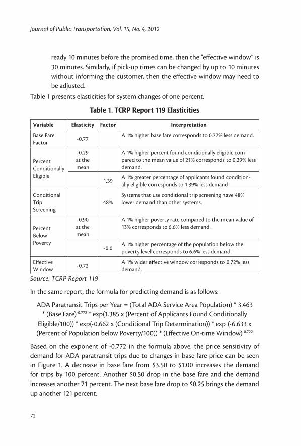
Journal of Public Transportation, Vol. 15, No. 4, 2012
72
ready 10 minutes before the promised time, then the “effective window” is 30 minutes. Similarly, if pick-up times can be changed by up to 10 minutes without informing the customer, then the effective window may need to be adjusted.
Table 1 presents elasticities for system changes of one percent.
Table 1. TCRP Report 119 Elasticities
Variable Elasticity Factor Interpretation
Base Fare Factor
-0.77A 1% higher base fare corresponds to 0.77% less demand.
Percent Conditionally Eligible
-0.29at the mean
A 1% higher percent found conditionally eligible com-pared to the mean value of 21% corresponds to 0.29% less demand.
1.39A 1% greater percentage of applicants found condition-ally eligible corresponds to 1.39% less demand.
Conditional Trip Screening
48%Systems that use conditional trip screening have 48% lower demand than other systems.
Percent Below Poverty
-0.90at the mean
A 1% higher poverty rate compared to the mean value of 13% corresponds to 6.6% less demand.
-6.6A 1% higher percentage of the population below the poverty level corresponds to 6.6% less demand.
Effective Window
-0.72A 1% wider effective window corresponds to 0.72% less demand.
Source: TCRP Report 119
In the same report, the formula for predicting demand is as follows:
ADA Paratransit Trips per Year = (Total ADA Service Area Population) * 3.463 * (Base Fare)-0.772 * exp(1.385 x (Percent of Applicants Found Conditionally
Eligible/100)) * exp(-0.662 x (Conditional Trip Determination)) * exp (-6.633 x (Percent of Population below Poverty/100)) * (Effective On-time Window)-0.722
Based on the exponent of -0.772 in the formula above, the price sensitivity of demand for ADA paratransit trips due to changes in base fare price can be seen in Figure 1. A decrease in base fare from $3.50 to $1.00 increases the demand for trips by 100 percent. Another $0.50 drop in the base fare and the demand increases another 71 percent. The next base fare drop to $0.25 brings the demand up another 121 percent.

73
Cost Estimation of Fare-Free ADA Complementary Paratransit Service in Illinois
Figure 1. TCRP Report 119 demand curve
The implication of the TCRP demand curve is that as base fare closes in the neighbor-hood of a fare-free policy, the ADA demand for paratransit trips becomes “infinitely large,” which is obviously absurd given the supply constraints. Besides, it would be difficult to justify the huge number of eligible paratransit ADA riders or the dramatic change in trip making corresponding to such “infinite” demand for trips.
The veracity of this argument can be readily demonstrated by inserting different values in the spreadsheet tool that accompanies the TCRP report (onlinepubs.trb.org/onlinepubs/tcrp/tcrp_rpt_119Tool.xls). For example, in an area with 1,000,000 population, the predicted annual ADA ridership is 18,581,500 trips for a fare-free policy (actually, the fare was set to $0.01 because the TCRP model is not defined at $0 fare), while doubling the area’s population increases the ADA annual trips to 37,162,999, which is almost 10 times the number of trips the New York City Transit Authority currently provides.
Clearly, the TCRP demand curve as presented cannot be used to estimate the impact of fare-free policies. In fairness, that was not the purpose of the TCRP demand curve, the estimation of which was partially based on a base fare range between $0.50 and $3.50 among the 28 transit properties studied.
TCRP Demand Curve AdjustmentGiven the need to obtain a reasonable measure to assess the demand for trips due to a fare-free policy, we decided to adjust the previous TCRP demand curve. Three reasons led us to such a decision: (a) uncertainty regarding availability of local
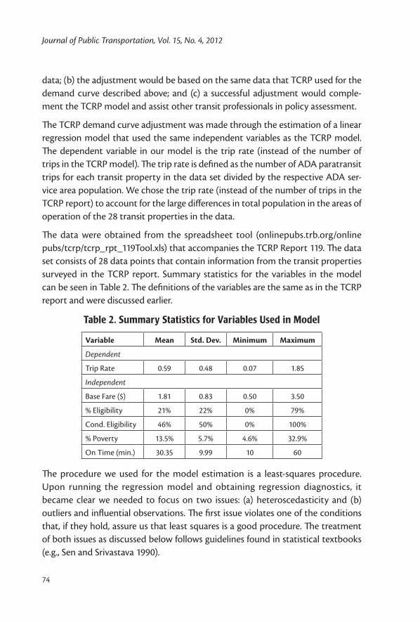
Journal of Public Transportation, Vol. 15, No. 4, 2012
74
data; (b) the adjustment would be based on the same data that TCRP used for the demand curve described above; and (c) a successful adjustment would comple-ment the TCRP model and assist other transit professionals in policy assessment.
The TCRP demand curve adjustment was made through the estimation of a linear regression model that used the same independent variables as the TCRP model. The dependent variable in our model is the trip rate (instead of the number of trips in the TCRP model). The trip rate is defined as the number of ADA paratransit trips for each transit property in the data set divided by the respective ADA ser-vice area population. We chose the trip rate (instead of the number of trips in the TCRP report) to account for the large differences in total population in the areas of operation of the 28 transit properties in the data.
The data were obtained from the spreadsheet tool (onlinepubs.trb.org/online pubs/tcrp/tcrp_rpt_119Tool.xls) that accompanies the TCRP Report 119. The data set consists of 28 data points that contain information from the transit properties surveyed in the TCRP report. Summary statistics for the variables in the model can be seen in Table 2. The definitions of the variables are the same as in the TCRP report and were discussed earlier.
Table 2. Summary Statistics for Variables Used in Model
Variable Mean Std. Dev. Minimum Maximum
Dependent
Trip Rate 0.59 0.48 0.07 1.85
Independent
Base Fare ($) 1.81 0.83 0.50 3.50
% Eligibility 21% 22% 0% 79%
Cond. Eligibility 46% 50% 0% 100%
% Poverty 13.5% 5.7% 4.6% 32.9%
On Time (min.) 30.35 9.99 10 60
The procedure we used for the model estimation is a least-squares procedure. Upon running the regression model and obtaining regression diagnostics, it became clear we needed to focus on two issues: (a) heteroscedasticity and (b) outliers and influential observations. The first issue violates one of the conditions that, if they hold, assure us that least squares is a good procedure. The treatment of both issues as discussed below follows guidelines found in statistical textbooks (e.g., Sen and Srivastava 1990).
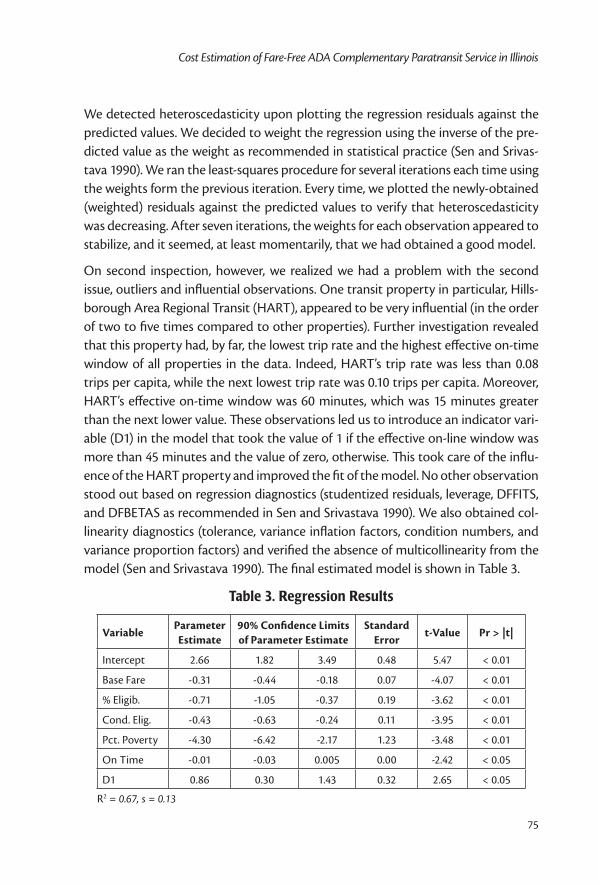
75
Cost Estimation of Fare-Free ADA Complementary Paratransit Service in Illinois
We detected heteroscedasticity upon plotting the regression residuals against the predicted values. We decided to weight the regression using the inverse of the pre-dicted value as the weight as recommended in statistical practice (Sen and Srivas-tava 1990). We ran the least-squares procedure for several iterations each time using the weights form the previous iteration. Every time, we plotted the newly-obtained (weighted) residuals against the predicted values to verify that heteroscedasticity was decreasing. After seven iterations, the weights for each observation appeared to stabilize, and it seemed, at least momentarily, that we had obtained a good model.
On second inspection, however, we realized we had a problem with the second issue, outliers and influential observations. One transit property in particular, Hills-borough Area Regional Transit (HART), appeared to be very influential (in the order of two to five times compared to other properties). Further investigation revealed that this property had, by far, the lowest trip rate and the highest effective on-time window of all properties in the data. Indeed, HART’s trip rate was less than 0.08 trips per capita, while the next lowest trip rate was 0.10 trips per capita. Moreover, HART’s effective on-time window was 60 minutes, which was 15 minutes greater than the next lower value. These observations led us to introduce an indicator vari-able (D1) in the model that took the value of 1 if the effective on-line window was more than 45 minutes and the value of zero, otherwise. This took care of the influ-ence of the HART property and improved the fit of the model. No other observation stood out based on regression diagnostics (studentized residuals, leverage, DFFITS, and DFBETAS as recommended in Sen and Srivastava 1990). We also obtained col-linearity diagnostics (tolerance, variance inflation factors, condition numbers, and variance proportion factors) and verified the absence of multicollinearity from the model (Sen and Srivastava 1990). The final estimated model is shown in Table 3.
Table 3. Regression Results
VariableParameter Estimate
90% Confidence Limits of Parameter Estimate
Standard Error
t-Value Pr > |t|
Intercept 2.66 1.82 3.49 0.48 5.47 < 0.01
Base Fare -0.31 -0.44 -0.18 0.07 -4.07 < 0.01
% Eligib. -0.71 -1.05 -0.37 0.19 -3.62 < 0.01
Cond. Elig. -0.43 -0.63 -0.24 0.11 -3.95 < 0.01
Pct. Poverty -4.30 -6.42 -2.17 1.23 -3.48 < 0.01
On Time -0.01 -0.03 0.005 0.00 -2.42 < 0.05
D1 0.86 0.30 1.43 0.32 2.65 < 0.05
R2 = 0.67, s = 0.13
Journal of Public Transportation, Vol. 15, No. 4, 2012
76
All of the coefficients are significant at the 95% confidence level. The model has a reasonable goodness of fit as measured by R-squared with 67 percent of variation in the ADA paratransit trip rate explained. The following observations can be made by examining the results for each variable in the model:
• The significant intercept term gives the predicted trip rate when all other variables are set to zero. This has no practical meaning.
• The fare coefficient implies that every drop in the base fare by $1 would increase ridership by 0.31 trips per capita (all other variables are held con-stant).
• Ridership decreases with the percent of applicants found conditionally ADA-eligible. Systems that have higher percentages of applicants found conditionally-eligible (rather than fully-eligible or eligible without conditions) have lower demand.
• Conditional trip screening reduces paratransit usage. Given that this is a 0/1 variable, the coefficient of this variable would indicate that systems that use conditional trip screening have 43 percent less ridership than systems that do not use conditional trip screening. A possible explanation of this is that riders reduce their requests based on the conditions they have been given or based on experiences in which they have requested trips and been turned down for trip-specific eligibility reasons. Another reason might be that sys-tems that use conditional trip screening also have more rigorous eligibility screening practices in general in ways not captured by the percentage of applicants found fully or conditionally eligible (Koffman 2007).
• Trip making decreases at higher poverty rates. Recall that this variable measures the total area-wide poverty rate, not the rate of poverty among people with disabilities. In general, people with higher income travel more than people with lower income. It is also likely that communities with higher poverty rates will have fewer available activities that generate travel than more affluent communities.
• Longer effective windows reduce trip making, but its effect is not pro-nounced.
Implications of Model Results for a Free Fare PolicyThe parameter estimate of the base fare is -0.31 with a 90 percent confidence inter-val of [-0.44, -0.18]. As a result, and assuming the other variables in the model are held constant, reducing the base fare from $3 to $0 would increase the average trip
77
Cost Estimation of Fare-Free ADA Complementary Paratransit Service in Illinois
rate by (3 ×0.31 = 0.93 trips per capita) or a percentage increase (at the mean trip rate of 0.59 in Table 2) of ([0.59 + 0.93]/0.59 = 257%). Moreover, 90 percent of the time, the trip rate is expected to increase (at the mean) between 191 and 323 per-cent. With the additional assumption that the total population in the service area will remain unchanged in the short term, the findings regarding trip rates translate directly into the demand for ADA complementary paratransit trips.
Note that the predicted trip rate increase does not necessarily mean that paratran-sit riders would start making more trips enticed by the free-fare policy (although this should not be excluded at least to some extent). Such an increase along with increases due to latent demand and demand shift from fixed-route services (as mentioned earlier in this paper) would increase the total number of ADA para-transit trips. As a result, given that the total population (the denominator) remains fixed, the trips-per-capita value increases.
It would also be worth noting that factors such as inflation and fare policy changes in the future could affect the calculus of the cost impacts of a free-fare policy. Additionally, a potential demand shift from fixed-route services could also affect such cost impacts. These factors could not be addressed in this paper. Moreover, using an average cost per trip as the basis for estimating the predicted costs over the entire spectrum of anticipated demand increase may prove to be a high-end estimate of total costs because of economies of scale in the provision of free-fare services.
Table 4 summarizes the impact of the zero-fare policy for different parts of the Chicago region. It is important to note that such impacts can be reasonably antici-pated under two provisions:
• Pace ADA paratransit operations are similar (in terms of eligibility and effective on-time window) from those in the transit agencies included in the data set we analyzed. Indeed, the RTA indicates 100 percent eligibility and a 20-minute on-time window (RTA 2006), which is within the ranges reported in TCRP Report 119.
• The percentage of people in households with incomes below the poverty rate in the Chicago area is similar to those from other parts of the country in the data set analyzed. Indeed, the poverty rate in Illinois ranges from 4 to 19 percent compared to the 3 to 33 percent range reported in TCRP Report 119.

Journal of Public Transportation, Vol. 15, No. 4, 2012
78
Table 4. Expected Demand Increase in Chicago Area
Region/CountyCurrent
FareExpected Annual Demand Increase
Range of Annual Demand Increase (90% Certainty)
Cook* & DuPage Counties $3.00 150% 129% to 171%
Lake, Kane, Will & McHenry Counties
$2.50 141% 124% to 159%
City of Chicago $2.25 137% 121% to 153%
*excluding the City of Chicago
In the Chicago region, the current ADA trip rate reported by Pace is 1.85. Consid-ering the fare differential in separate parts of the region, the range of impacts on demand of a free-fare policy is reported in Table 4. Note that the larger the drop from a current base-fare value to a zero-fare policy, the larger the range (uncer-tainty) of the impact on the demand for ADA trips.
Perhaps a few words of caution are in order here. The particular model specifica-tion does not prevent estimating negative trip rates for certain combinations of the independent factors. Fortunately, this was not the case with the data analyzed; all predicted rates were positive, with 26 out of 28 trip rates within the prediction interval. In addition, many factors that could potentially affect the ADA demand are not included in the model and, therefore, their impact should be corroborated from other sources. Meanwhile, the model above is a reasonable approach to quan-tify the impacts of a zero-fare policy on ADA paratransit demand.
Cost Estimation of a Free Fare PolicyAverage Cost Per TripThe cost to provide origin-to-destination ADA special services varies with the type of service provided, vehicle characteristics, the vendor, and the type of contract. In northeastern Illinois, Pace contracts for service in both the city and suburbs. The majority of the systems in the rest of the state contract with private vendors and, in some cases, in conjunction with their dial-a-ride for the general public and older adults. Table 5 shows the average cost per trip as reported by the transit agencies for 2007. Note that the suburban cost in Table 5 includes a contract cost of $31.16 per trip plus an imputed capital cost of a paratransit vehicle of $0.94 per trip.
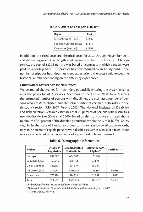
79
Cost Estimation of Fare-Free ADA Complementary Paratransit Service in Illinois
Table 5. Average Cost per ADA Trip
Region Cost
City of Chicago (Pace) $32.35
Suburban Chicago (Pace) $32.10
Downstate (average) $26.43
In addition, the cited costs are historical costs for 2007 through November 2011 and, depending on contract length, could increase in the future. For city of Chicago service, the cost of $32.35 per trip was based on contracts in which vendors were paid on a per-trip basis. This practice has now changed to an hourly basis. If the number of trips per hour does not meet expectations, the costs could exceed the historical number depending on the efficiency experienced.
Estimation of Market Size for New RidersWe estimated the market for new riders potentially entering the system given a zero fare policy for ADA services. According to the Census 2000, Table 6 shows the estimated number of persons with disabilities, the estimated number of per-sons who are ADA-eligible, and the total number of certified ADA riders in the six-county region (RTA 2007; Perone 2002). The National Institute on Disability and Rehabilitation Research estimates that 20 percent of persons with disabilities use mobility devices (Kaye et al. 2000). Based on this statistic, we estimated that a minimum of 20 percent of the disabled population within the ¾-mile buffer is ADA eligible. In the state of Illinois, according to transit agency certification records, only 18.7 percent of eligible persons with disabilities within ¾ mile of a fixed-route service are certified, which is evidence of a great deal of latent demand.
Table 6. Demographic Information
RegionDisabled*
PopulationDisabled within
¾ Mile BufferEstimated ADA
Eligible**Certified***
Chicago 604,602 604,602 120,920 -
Suburban Cook 368,956 368,353 73,671 -
Collar Counties 318,183 291,519 58,304 -
Chicago Region 1,291,741 1,264,474 252,895 42,038
Downstate 707,976 314,759 62,952 14,421
Total 1,999,717 1,579,233 315,847 56,459
*Disabled populations are estimated from Census SF3 data ** National Institute on Disability and Rehabilitation Research (Kaye et al. 2000) ***Transit Agency Records
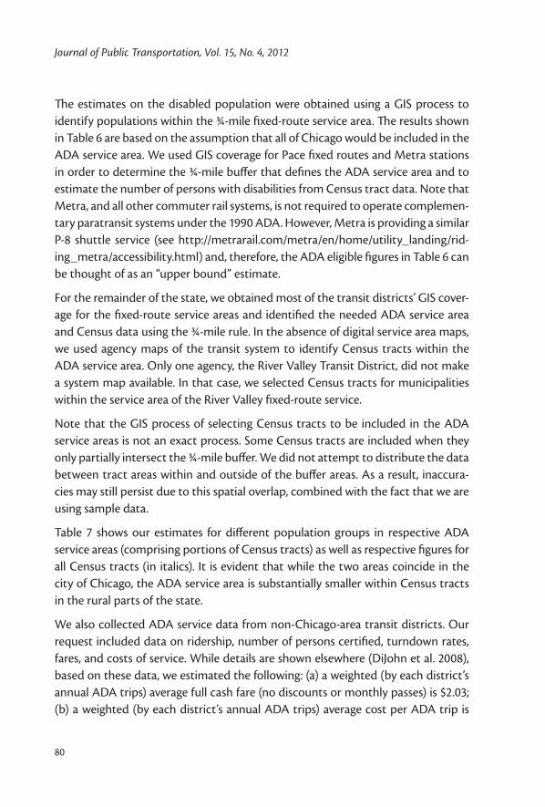
Journal of Public Transportation, Vol. 15, No. 4, 2012
80
The estimates on the disabled population were obtained using a GIS process to identify populations within the ¾-mile fixed-route service area. The results shown in Table 6 are based on the assumption that all of Chicago would be included in the ADA service area. We used GIS coverage for Pace fixed routes and Metra stations in order to determine the ¾-mile buffer that defines the ADA service area and to estimate the number of persons with disabilities from Census tract data. Note that Metra, and all other commuter rail systems, is not required to operate complemen-tary paratransit systems under the 1990 ADA. However, Metra is providing a similar P-8 shuttle service (see http://metrarail.com/metra/en/home/utility_landing/rid-ing_metra/accessibility.html) and, therefore, the ADA eligible figures in Table 6 can be thought of as an “upper bound” estimate.
For the remainder of the state, we obtained most of the transit districts’ GIS cover-age for the fixed-route service areas and identified the needed ADA service area and Census data using the ¾-mile rule. In the absence of digital service area maps, we used agency maps of the transit system to identify Census tracts within the ADA service area. Only one agency, the River Valley Transit District, did not make a system map available. In that case, we selected Census tracts for municipalities within the service area of the River Valley fixed-route service.
Note that the GIS process of selecting Census tracts to be included in the ADA service areas is not an exact process. Some Census tracts are included when they only partially intersect the ¾-mile buffer. We did not attempt to distribute the data between tract areas within and outside of the buffer areas. As a result, inaccura-cies may still persist due to this spatial overlap, combined with the fact that we are using sample data.
Table 7 shows our estimates for different population groups in respective ADA service areas (comprising portions of Census tracts) as well as respective figures for all Census tracts (in italics). It is evident that while the two areas coincide in the city of Chicago, the ADA service area is substantially smaller within Census tracts in the rural parts of the state.
We also collected ADA service data from non-Chicago-area transit districts. Our request included data on ridership, number of persons certified, turndown rates, fares, and costs of service. While details are shown elsewhere (DiJohn et al. 2008), based on these data, we estimated the following: (a) a weighted (by each district’s annual ADA trips) average full cash fare (no discounts or monthly passes) is $2.03; (b) a weighted (by each district’s annual ADA trips) average cost per ADA trip is
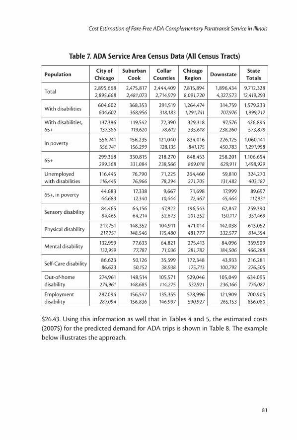
81
Cost Estimation of Fare-Free ADA Complementary Paratransit Service in Illinois
Table 7. ADA Service Area Census Data (All Census Tracts)
PopulationCity of
ChicagoSuburban
CookCollar
CountiesChicago Region
DownstateState Totals
Total2,895,6682,895,668
2,475,8172,481,073
2,444,4092,714,979
7,815,8948,091,720
1,896,4344,327,573
9,712,32812,419,293
With disabilities604,602604,602
368,353368,956
291,519318,183
1,264,4741,291,741
314,759707,976
1,579,2331,999,717
With disabilities, 65+
137,386137,386
119,542119,620
72,39078,612
329,318335,618
97,576238,260
426,894573,878
In poverty556,741556,741
156,235156,299
121,040128,135
834,016841,175
226,125450,783
1,060,1411,291,958
65+299,368299,368
330,815331,084
218,270238,566
848,453869,018
258,201629,911
1,106,6541,498,929
Unemployed with disabilities
116,445116,445
76,79076,966
71,22578,294
264,460271,705
59,810131,482
324,270403,187
65+, in poverty44,68344,683
17,33817,340
9,66710,444
71,69872,467
17,99945,464
89,697117,931
Sensory disability84,46584,465
64,15664,214
47,92252,673
196,543201,352
62,847150,117
259,390351,469
Physical disability217,751217,751
148,352148,546
104,911115,480
471,014481,777
142,038332,577
613,052814,354
Mental disability132,959132,959
77,63377,787
64,82171,036
275,413281,782
84,096184,506
359,509466,288
Self-Care disability86,62386,623
50,12650,152
35,59938,938
172,348175,713
43,933100,792
216,281276,505
Out-of-home disability
274,961274,961
148,514148,685
105,571114,275
529,046537,921
105,049236,166
634,095774,087
Employment disability
287,094287,094
156,547156,836
135,355146,997
578,996590,927
121,909265,153
700,905856,080
$26.43. Using this information as well that in Tables 4 and 5, the estimated costs (2007$) for the predicted demand for ADA trips is shown in Table 8. The example below illustrates the approach.
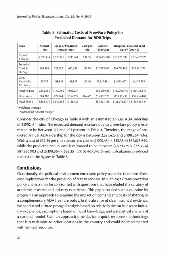
Journal of Public Transportation, Vol. 15, No. 4, 2012
82
Table 8. Estimated Costs of Free-Fare Policy for Predicted Demand for ADA Trips
Area Annual Trips
Range of Predicted Annual Trips
Cost per Trip
Current Total Cost
Range in Predicted Total Cost** (2007 $)
City of Chicago
2,090,434 2,529,425 3,198,364 $32.35 $67,625,540 $81,826,903 $103,467,076
Suburban Cook & DuPage
404,288 521,532 691,332 $32.10 $12,977,645 $16,741,162 $22,191,773
Lake, Kane Will, McHenry
87,772 108,837 139,557 $32.10 $2,817,481 $3,493,677 $4,479,795
Total Region 2,582,494 3,159,794 4,029,254 - $83,420,666 $102,061,742 $130,138,644
Downstate 604,280 827,864 1,154,175 $26.43* $15,971,120 $21,880,435 $30,504,840
Total Illinois 3,186,774 3,987,658 5,183,429 - $99,391,786 $123,942,177 $160,643,484
*weighted average**rounded to nearest integer
Consider the city of Chicago in Table 8 with an estimated annual ADA ridership of 2,090,434 rides. The expected demand increase due to a free-fare policy is esti-mated to be between 121 and 153 percent in Table 4. Therefore, the range of pre-dicted annual ADA ridership for the city is between 2,529,425 and 3,198,364 rides. With a cost of $32.35 per trip, the current cost is (2,090,434 × $32.35 =) $67,625,540, while the predicted annual cost is estimated to be between (2,529,425 × $32.35 =) $81,826,903 and (3,198,364 × $32.35 =) $103,467,076. Similar calculations produced the rest of the figures in Table 8.
ConclusionsOccasionally, the political environment entertains policy scenarios that have direct cost implications for the provision of transit services. In such cases, transportation policy analysts may be confronted with questions that have eluded the scrutiny of academic research and industry experience. This paper tackled such a question by proposing an approach to examine the impact on demand and costs of shifting to a complementary ADA free-fare policy. In the absence of clear historical evidence, we conducted a three-pronged analysis based on relatively similar but scant indus-try experience, assumptions based on local knowledge, and a statistical analysis of a national model. Such an approach provides for a quick response methodology that is transferable to other locations in the country and could be implemented with limited resources.
83
Cost Estimation of Fare-Free ADA Complementary Paratransit Service in Illinois
In doing so, the methodology complements the work conducted for TCRP Report 119 by examining the fare elasticity of demand in the neighborhood of free fare. The industry experience and local knowledge about ADA complementary opera-tions, on the other hand, allowed us to “validate” the answers obtained from the statistical analysis. As a result, we are confident that the predicted range of impacts on demand and costs are sufficiently reasonable to use in a high-level planning analysis of “what-if” scenarios.
References
American Public Transportation Association. 1991. Effects of fare changes on bus ridership. Washington, DC. http://www.apta.com/research/info/online/elastic.cfm (accessed December 2011).
AppalCart. 2011. Fact sheet and press releases, 2006 and 2007. http://www.appal-cart.appstate.edu/EN/US/ (accessed December 2011).
Chicago Transit Authority. 2011. 2005 vs. 2006 performance indicators. http://www.transitchicago.com/news/motion/board/122046perfind4Q2006.pdf (accessed December 2011).
DiJohn, J., P. Metaxatos, L. Dirks, and K. Allen. 2008. ADA special services: Price elas-ticity for the provision of free service in the state of Illinois. Final report. Illinois Department of Transportation Division of Public and Intermodal Transporta-tion. May 14, 2008.
Doxsey, L. B., and B. D. Spear (1981). Free-fare transit: Some empirical findings. Transportation Research Record 799: 47–49.
Kaye, H., S., T. Kang, and M. P. Laplante. 2000. Mobility device use in the United States: Disability statistics report. University of California, San Francisco for National Institute on Disability and Rehabilitation, June 2000.
Koffman, D., D. Lewis, D. Chia, J. Burkhardt, and M. Bradley. 2007. Improving ADA complementary paratransit demand estimation. Transit Cooperative Research Program, Report 119.
McCollom, B. E., and R. H. Pratt. 2004. Traveler response to transportation system changes: Chapter 12 – transit pricing and fares. Transit Cooperative Research Program, Report 95.
Journal of Public Transportation, Vol. 15, No. 4, 2012
84
Pace Suburban Bus. 2007. Suburban service and regional ADA budget results. Arlington Heights, Illinois, November 2007.
Perone, J. 2002. Advantages and disadvantages of fare-free transit policy. National Center for Transit Research, Report No. 473-1333. Tampa, FL., October 2002.
Perone, J., and J. Volinski. 2003. Fare, free or something in between? Center for Urban Transportation Research, University of South Florida, Tampa, FL.
Pratt, R. H. 2000. Traveler response to transportation system changes. Transit Cooperative Research Program, Web Document 12. Interim Handbook.
Regional Transportation Authority. 2007. Connecting communities through coor-dination: The Northeastern Illinois Coordinated Public Transit—Human Ser-vices Transportation Plan (HSTP). September, 2007, Chicago, Illinois.
Regional Transportation Authority, Chicago Transit Authority and Pace Suburban Bus Service, 2006. Regional ADA paratransit plan for persons with disabilities. January 2006, Chicago, Illinois.
Sen, A., and M. Srivastava, 1990. Regression Analysis: Theory, Methods and Applica-tions. New York: Springer-Verlag.
Spielberg, F,. and R. H. Pratt. 2004. Traveler response to transportation system changes: Chapter 6—Demand responsive/ADA. Transit Cooperative Research Program, Report 95.
Studenmund, A. H., and D. Connor. 1982. The free-fare transit experiment. Trans-portation Research 15(4): 261–270.
U.S. Government Printing Office via GPO Access. 2011. Transportation Services for Individuals with Disabilities. 49CFR37, p. 440. http://www.fta.dot.gov/civil-rights/ada/civil_rights_3906.html (accessed December 2011).
West, J. 1996. Implementing the Americans with Disabilities Act. Blackwell Publish-ing, Cambridge, MA.
About the Authors
Paul Metaxatos ([email protected]) is Associate Director for Research Programs and Research Assistant Professor in the Urban Transportation Center, University of Illinois at Chicago. He has conducted numerous transit planning studies in Illinois.

85
Cost Estimation of Fare-Free ADA Complementary Paratransit Service in Illinois
He most recently advised the Regional Transportation Authority in Chicago about the ridership and cost implications of an older adult free-ride program.
Lise Dirks ([email protected]) is Senior Associate in the Urban Transportation Center, University of Illinois at Chicago. She specializes in GIS development and has worked on numerous transit planning studies in Illinois.

Journal of Public Transportation, Vol. 15, No. 4, 2012
86
87
Transit Operator Evaluation of Three Wheelchair Securement Systems
Transit Operator Evaluation of Three Wheelchair Securement Systems in a
Large Accessible Transit VehicleLinda van Roosmalen, Douglas Hobson, Patricia Karg, Emily DeLeo, Erik Porach
University of Pittsburgh
Abstract
The safety, ease of use, and independent use of three wheelchair securement systems and three different types of wheeled mobility devices (WhMD), including a manual wheelchair, a powered wheelchair, and a three-wheeled scooter, were evaluated by eight vehicle operators of a large accessible public transit vehicle (LATV). The secure-ment systems included a forward-facing four-point tiedown system, a prototype forward-facing autodocking system, and a prototype rear-facing-wheelchair pas-senger (RF-WP) system. The eight LATV operators transported wheelchair-seated passengers in each wheelchair securement system, after which they completed a questionnaire.
Operators responded generally positively to the autodocking and RF-WP systems because they were observed by the drivers to be quicker and easier to use and allowed more independent use by wheelchair-seated passengers compared to the four-point tiedown system. From all three securement systems, operators favored the forward-facing autodocking system, because no assistance from operators is required to use it and most users preferred the forward-facing orientation in the vehicle. The autodocking system was perceived to be safe and easy to use by wheelchair- and scooter-seated passengers. These study results promote the need for alternative and improved securement systems that can be used by wheelchair and scooter-seated
Journal of Public Transportation, Vol. 15, No. 4, 2012
88
passengers that travel in LATVs in forward- or rearward-facing directions. Ideally, future securement solutions should not require assistance from LATV operators for their operation and should allow wheelchair- and scooter-seated passengers to ride public transportation safely and independently.
IntroductionIn the United States, the majority of public transportation vehicles have become accessible to individuals using wheeled mobility devices (WhMD). This is largely due to the U. S. Department of Transportation’s (DOT) Americans with Disabilities Act (ADA) regulations requiring public transportation to be fully accessible to individuals with disabilities (U. S. DOT 2010). Lifts and ramps provide an indepen-dent means to board and exit motor vehicles, and wheelchair securement stations equipped with wheelchair tiedown and occupant restraint systems (WTORS) are commonly installed so that operators can safely secure wheelchairs and restrain wheelchair-seated passengers. However, section 37.5 of DOT’s ADA stipulates that vehicle operators cannot require the use of occupant restraints by wheelchair pas-sengers unless transit authorities have adopted a written policy that mandates the use of occupant restraints (U. S. DOT 2010).
Current Status of on WTORS used on LATVsIn general, WTORS in large, accessible transit vehicles (LATV) cannot be indepen-dently used by wheelchair users and require assistance from a vehicle operator. Several studies have investigated the use and, more importantly, the non-use of WTORS by operators when they transport wheelchair-seated individuals in LATVs (Abelson et al. 2008; Foreman and Hardin 2001). The Foreman and Hardin (2001) survey focused on challenges faced by operators in LATVs related to WTORS. They found that scooters, in particular, are difficult to secure and often cannot be adequately secured due to a lack of identifiable securement points and limitations of currently-installed wheelchair securement technologies that require narrow frame members for looping around webbing-type straps and hardware. In fact, 46 percent of survey respondents reported that operators encounter difficulties when attempting to secure three- and four-wheel scooters (Foreman and Hardin 2001). Current WTORS also require operators to leave their driver station and to come in close contact with passengers (Foreman and Hardin 2001). Tiedown sys-tems using retractor technology are easy to tighten; however, tiedowns with the traditional manual adjustment buckles are time-consuming to use (Blower et al. 2005). Boarding a wheelchair in combination with a lengthy securement process
89
Transit Operator Evaluation of Three Wheelchair Securement Systems
conflicts with the daily struggle for vehicle operators to meet bus route schedules. Finally, wheelchair-seated passengers and operators complain about dirty, twisted, or missing tiedown straps and occupant restraints (Abelson et al. 2008).
ADA defines a wheelchair as a mobility aid belonging to any class of three- or four-wheeled devices, usable indoors, designed for and used by individuals with mobil-ity impairments, whether operated manually or powered. A common wheelchair does not exceed 30 inches in width and 48 inches in length measured two inches above the ground and does not weigh more than 600 pounds when occupied (U.S. DOT 2010). Non-common wheelchairs that do not fit the definition of a com-mon wheelchair can make the securement process difficult and sometimes even impossible (Foreman and Hardin 2001; Hardin et al. 2002; Project Action 2008). An additional complication is that long and narrow WhMDs such as scooters have a high center of gravity in combination with a narrow wheelbase and may therefore tip over when not properly secured. A study done by Turkovich et al. (2011) dem-onstrated that common scooters and wheelchairs tip over during normal vehicle maneuvers (such as turning and braking) in an LATV. It is not uncommon in other countries for transit systems to prohibit the transport of over-size mobility devices and scooters on LATVs (United Kingdom Department for Transport 2006). In the U.S., however, ADA regulations prohibit discrimination and require transit authori-ties to accommodate any individual seated in a common wheelchair. More and more WhMDs are being produced that comply with the RESNA WC19 voluntary industry safety standard for wheelchairs used as seats in motor vehicles. Compli-ance with the standard improves safety and the ease of application of four-point strap-type tiedowns by requiring four easily-identifiable securement points on the wheelchair (ANSI/RESNA 2001). These WC19 wheelchairs are crash-tested, and their four securement points are clearly labeled and attached or integrated into the wheelchair or seating frame. WC19 wheelchairs also have anchorage points for a pelvic restraint that has been designed to protect wheelchair-seated occupants riding in a motor vehicle and are rated for accommodation of vehicle-anchored occupant restraints. The use of WC19 wheelchairs, however, is limited at this point in time, and challenges with securement use remain an issue.
There are additional issues with the current vehicle-installed WTORS that affect how LATV operators adhere to safe and best practices. Some wheelchair-seated passengers refuse to have their wheelchair secured to the vehicle. Dealing with unwilling passengers makes operator adherence to company policy and follow-ing best practices, i.e., securing wheelchairs and restraining occupants, difficult.
Journal of Public Transportation, Vol. 15, No. 4, 2012
90
Inconsistent policies and inconsistent reinforcement of policies may result either in trip denial for wheelchair passengers unwilling to be secured or wheelchair passengers traveling unsafely. Insufficient operator training in combination with non-common wheelchairs onboard LATVs can also result in poor wheelchair securement practices and an increased injury risk to wheelchair-seated and ambu-latory passengers (Foreman and Hardin 2001). An additional concern is the current confusion and lack of knowledge that exists among LATV operators as to whether or not wheelchair passengers must wear a seatbelt and/or have their wheelchair secured, especially since other ambulatory passengers often do not require safety measures such as seatbelts on board LATVs (Foreman and Hardin 2001; Hardin et al. 2002). Although the use of WTORS may minimize risk to WhMD passengers and others on board LATVs, 16 percent of respondents in an operator study done by Foreman and Hardin (2001) reported injuries that did not occur to wheelchair users but to operators as a result of using WTORS on WhMDs. These occupational injuries included back strains, arm and shoulder injuries, carpel tunnel syndrome, cuts, scrapes and bruises. Improved WTORS are being developed to address some of these issues.
Improvements to WTORSOregon State University was one of the first to develop an operator-independent securement solution for wheelchair passengers that requires a wheelchair-mounted bracket (adaptor) that engages with a vehicle-mounted docking device (Hobson and van Roosmalen 2007). The concept of autodocking was further explored at the University of Pittsburgh (Hobson and van Roosmalen 2007). This concept was based on a standardized universal interface geometry that is specified in ISO 10542 and RESNA WC19 standards (ISO 2005). Autodocking technologies have yet to become commercially available and successful. Success depends greatly on the mutual efforts of wheelchair manufacturers (to produce wheelchairs with universal [ISO] adaptors) and transit organizations (to install ISO-compliant dock-ing devices in LATVs).
Another passive securement solution has been adopted in European public transit and some U.S. and Canadian public transit systems (Hunter-Zaworski 2004). This technology can be identified by its rear-facing approach to containing occupied WhMDs in LATVs (RF-WP systems). This system, in its simplest form, consists of a padded area behind a (rear-facing) wheelchair user and usually includes an aisle-mounted structure to prevent tipping or swerving of WhMDs. This system is believed to be operator- and wheelchair-passenger friendly in that it allows inde-
91
Transit Operator Evaluation of Three Wheelchair Securement Systems
pendent operation by most WhMD passengers that board LATVs. A concern with currently used RF-WP systems is the insufficient lateral containment this system offers to WhMDs that are exposed to accelerations related to LATV turning.
Research remains ongoing to understand the safety of the various securement systems during normal and emergency driving maneuvers in LATVs (Turkovich et al. 2011; van Roosmalen et al. 2011). Shaw (2008) found that public transportation is a very safe mode of transportation and accidents due to vehicle crashes are rare. However, incidents related to normal vehicle maneuvering are more frequent and have been reported by several researchers in the field (Frost and Bertocci 2009, 2010; Songer et al. 2004). Incidents in LATVs are commonly due to poor wheelchair securement and/or restraint of wheelchair- and scooter-seated passengers (Frost and Bertocci 2009).
This study’s long-term goal is to minimize wheelchair-related incidents and lower risk of injury among WhMD-seated passengers traveling on LATVs by providing guidance on securement and restraint design approaches that will increase use. It also aims to listen to the voice of the customer (operators, passengers) when selecting technologies for the fast pace environment of modern public transporta-tion. This study is part of a broader study where wheelchair- and scooter-seated individuals were surveyed and asked for their perceived safety, comfort, and inde-pendence when using three types of wheelchair securement stations on board an LATV (Turkovich et al. 2009; van Roosmalen et al. 2011). The results in this publication are focused on operators of LATVs and their perceived ease of use of three types of wheelchair securement stations. Findings from this study clarify the preferred operator and wheelchair user responsibilities with respect to WTORS and guides product designers in the improvement of existing and development of alternative wheelchair safety systems on board LATVs that meet operator needs and wheelchair-seated passenger needs.
ObjectiveThe perceived safety and usability of prototype autodocking and RF-WP systems was compared to a commercial four-point tiedown system by means of a survey. The objective was to learn LATV operators’ and operator trainers’ opinions on ways in which wheelchair securement systems can be improved to optimize system safety, usability, and operational feasibility in the LATV environment.
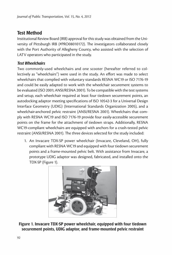
Journal of Public Transportation, Vol. 15, No. 4, 2012
92
Test MethodInstitutional Review Board (IRB) approval for this study was obtained from the Uni-versity of Pittsburgh IRB (#PRO08010172). The investigators collaborated closely with the Port Authority of Allegheny County, who assisted with the selection of LATV operators who participated in the study.
Test WheelchairsTwo commonly-used wheelchairs and one scooter (hereafter referred to col-lectively as “wheelchairs”) were used in the study. An effort was made to select wheelchairs that complied with voluntary standards RESNA WC19 or ISO 7176-19 and could be easily adapted to work with the wheelchair securement systems to be evaluated (ISO 2001; ANSI/RESNA 2001). To be compatible with the test systems and setup, each wheelchair required at least four tiedown securement points, an autodocking adaptor meeting specifications of ISO 10542-3 for a Universal Design Interface Geometry (UDIG) (International Standards Organization 2005), and a wheelchair-anchored pelvic restraint (ANSI/RESNA 2001). Wheelchairs that com-ply with RESNA WC19 and ISO 7176-19 provide four easily-accessible securement points on the frame for the attachment of tiedown straps. Additionally, RESNA WC19-compliant wheelchairs are equipped with anchors for a crash-tested pelvic restraint (ANSI/RESNA 2001). The three devices selected for the study included:
1. An Invacare TDX-SP power wheelchair (Invacare, Cleveland, OH), fully compliant with RESNA WC19 and equipped with four tiedown securement points and a frame-mounted pelvic belt. With assistance from Invacare, a prototype UDIG adaptor was designed, fabricated, and installed onto the TDX-SP (Figure 1).
Figure 1. Invacare TDX-SP power wheelchair, equipped with four tiedown securement points, UDIG adaptor, and frame-mounted pelvic restraint
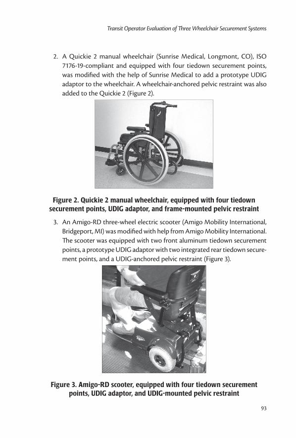
93
Transit Operator Evaluation of Three Wheelchair Securement Systems
2. A Quickie 2 manual wheelchair (Sunrise Medical, Longmont, CO), ISO 7176-19-compliant and equipped with four tiedown securement points, was modified with the help of Sunrise Medical to add a prototype UDIG adaptor to the wheelchair. A wheelchair-anchored pelvic restraint was also added to the Quickie 2 (Figure 2).
Figure 2. Quickie 2 manual wheelchair, equipped with four tiedown securement points, UDIG adaptor, and frame-mounted pelvic restraint
3. An Amigo-RD three-wheel electric scooter (Amigo Mobility International, Bridgeport, MI) was modified with help from Amigo Mobility International. The scooter was equipped with two front aluminum tiedown securement points, a prototype UDIG adaptor with two integrated rear tiedown secure-ment points, and a UDIG-anchored pelvic restraint (Figure 3).
Figure 3. Amigo-RD scooter, equipped with four tiedown securement points, UDIG adaptor, and UDIG-mounted pelvic restraint
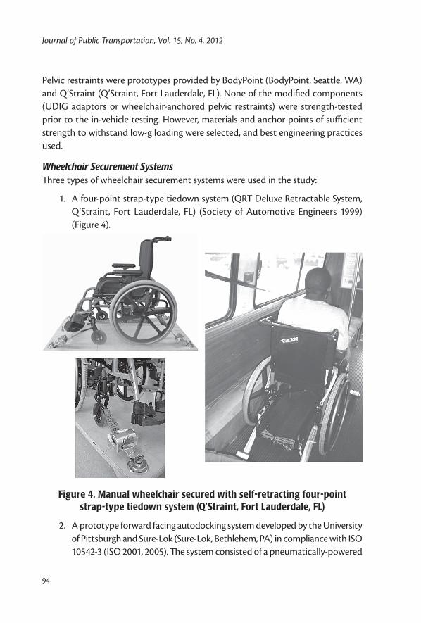
Journal of Public Transportation, Vol. 15, No. 4, 2012
94
Pelvic restraints were prototypes provided by BodyPoint (BodyPoint, Seattle, WA) and Q’Straint (Q’Straint, Fort Lauderdale, FL). None of the modified components (UDIG adaptors or wheelchair-anchored pelvic restraints) were strength-tested prior to the in-vehicle testing. However, materials and anchor points of sufficient strength to withstand low-g loading were selected, and best engineering practices used.
Wheelchair Securement SystemsThree types of wheelchair securement systems were used in the study:
1. A four-point strap-type tiedown system (QRT Deluxe Retractable System, Q’Straint, Fort Lauderdale, FL) (Society of Automotive Engineers 1999) (Figure 4).
Figure 4. Manual wheelchair secured with self-retracting four-point strap-type tiedown system (Q’Straint, Fort Lauderdale, FL)
2. A prototype forward facing autodocking system developed by the University of Pittsburgh and Sure-Lok (Sure-Lok, Bethlehem, PA) in compliance with ISO 10542-3 (ISO 2001, 2005). The system consisted of a pneumatically-powered
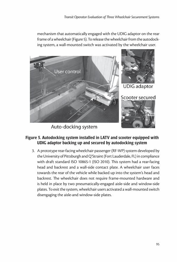
95
Transit Operator Evaluation of Three Wheelchair Securement Systems
mechanism that automatically engaged with the UDIG adaptor on the rear frame of a wheelchair (Figure 5). To release the wheelchair from the autodock-ing system, a wall-mounted switch was activated by the wheelchair user.
Figure 5. Autodocking system installed in LATV and scooter equipped with UDIG adaptor backing up and secured by autodocking system
3. A prototype rear-facing wheelchair passenger (RF-WP) system developed by the University of Pittsburgh and Q’Straint (Fort Lauderdale, FL) in compliance with draft standard ISO 10865-1 (ISO 2010). This system had a rear-facing head and backrest and a wall-side contact plate. A wheelchair user faces towards the rear of the vehicle while backed up into the system’s head and backrest. The wheelchair does not require frame-mounted hardware and is held in place by two pneumatically-engaged aisle-side and window-side plates. To exit the system, wheelchair users activated a wall-mounted switch disengaging the aisle-and window-side plates.
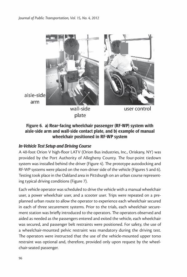
Journal of Public Transportation, Vol. 15, No. 4, 2012
96
Figure 6. a) Rear-facing wheelchair passenger (RF-WP) system with aisle-side arm and wall-side contact plate, and b) example of manual
wheelchair positioned in RF-WP system
In-Vehicle Test Setup and Driving CourseA 40-foot Orion V high-floor LATV (Orion Bus industries, Inc., Oriskany, NY) was provided by the Port Authority of Allegheny County. The four-point tiedown system was installed behind the driver (Figure 4). The prototype autodocking and RF-WP systems were placed on the non-driver side of the vehicle (Figures 5 and 6). Testing took place in the Oakland area in Pittsburgh on an urban course represent-ing typical driving conditions (Figure 7).
Each vehicle operator was scheduled to drive the vehicle with a manual wheelchair user, a power wheelchair user, and a scooter user. Trips were repeated on a pre-planned urban route to allow the operator to experience each wheelchair secured in each of three securement systems. Prior to the trials, each wheelchair secure-ment station was briefly introduced to the operators. The operators observed and aided as needed as the passengers entered and exited the vehicle, each wheelchair was secured, and passenger belt restraints were positioned. For safety, the use of a wheelchair-mounted pelvic restraint was mandatory during the driving test. The operators were instructed that the use of the vehicle-mounted upper torso restraint was optional and, therefore, provided only upon request by the wheel-chair-seated passenger.

97
Transit Operator Evaluation of Three Wheelchair Securement Systems
Figure 7. Map illustrating vehicle test route in Oakland
A questionnaire was developed and administered prior to and after comple-tion of the in-vehicle trials. The pre-test part of the survey covered questions on demographics and operator experience with existing wheelchair securement and occupant restraint systems. The post-test part of the survey asked for ratings on the ease of use, perceived safety, and independent use of the three different wheelchair securement systems. Operators were also asked to identify what they liked and disliked about each securement syste, which system they liked the best and least, and which was most and least safe for the passenger, was easiest and hardest to use, would be the most and least comfortable for the passenger, took the most and
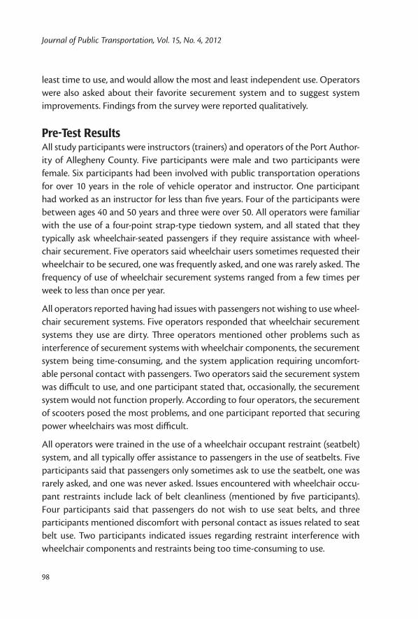
Journal of Public Transportation, Vol. 15, No. 4, 2012
98
least time to use, and would allow the most and least independent use. Operators were also asked about their favorite securement system and to suggest system improvements. Findings from the survey were reported qualitatively.
Pre-Test ResultsAll study participants were instructors (trainers) and operators of the Port Author-ity of Allegheny County. Five participants were male and two participants were female. Six participants had been involved with public transportation operations for over 10 years in the role of vehicle operator and instructor. One participant had worked as an instructor for less than five years. Four of the participants were between ages 40 and 50 years and three were over 50. All operators were familiar with the use of a four-point strap-type tiedown system, and all stated that they typically ask wheelchair-seated passengers if they require assistance with wheel-chair securement. Five operators said wheelchair users sometimes requested their wheelchair to be secured, one was frequently asked, and one was rarely asked. The frequency of use of wheelchair securement systems ranged from a few times per week to less than once per year.
All operators reported having had issues with passengers not wishing to use wheel-chair securement systems. Five operators responded that wheelchair securement systems they use are dirty. Three operators mentioned other problems such as interference of securement systems with wheelchair components, the securement system being time-consuming, and the system application requiring uncomfort-able personal contact with passengers. Two operators said the securement system was difficult to use, and one participant stated that, occasionally, the securement system would not function properly. According to four operators, the securement of scooters posed the most problems, and one participant reported that securing power wheelchairs was most difficult.
All operators were trained in the use of a wheelchair occupant restraint (seatbelt) system, and all typically offer assistance to passengers in the use of seatbelts. Five participants said that passengers only sometimes ask to use the seatbelt, one was rarely asked, and one was never asked. Issues encountered with wheelchair occu-pant restraints include lack of belt cleanliness (mentioned by five participants). Four participants said that passengers do not wish to use seat belts, and three participants mentioned discomfort with personal contact as issues related to seat belt use. Two participants indicated issues regarding restraint interference with wheelchair components and restraints being too time-consuming to use.
99
Transit Operator Evaluation of Three Wheelchair Securement Systems
Operators were asked if they ever felt uncomfortable or that it was unsafe for wheelchair-seated passengers during transit; four participants indicated rarely or never, and three participants said they occasionally felt this way. Participants felt uncomfortable when wheelchair-seated passengers refused to be secured or restrained or when they were unable to be secured or restrained properly due to mechanical issues with the wheelchair or WTORS. One operator mentioned being worried about other standing passengers falling onto or against a wheelchair-seated passenger.
When it comes to using the wheelchair ramp or lift when loading/unloading pas-sengers, four operators said they rarely or never felt uncomfortable or that is was unsafe. Three operators said they would sometimes feel uncomfortable or unsafe and listed ramp fatigue (due to frequent ramp use), ramp malfunction, and the risk of the wheelchair-seated patrons tipping over on the ramp or lift as reasons.
When asked the level of assistance they typically provide to wheelchair-seated passengers, five operators said they provided assistance with securing wheelchairs. Only one operator stated helping wheelchair-seated passengers with all five tasks listed (on/off ramp/lift, maneuvering into wheelchair station, securing the wheel-chair, applying seat belts, and transferring in/out of the wheelchair).
The main dislike operators reported was the unsanitary four-point tiedown station due to accumulating dirt on straps and belts. Operators suggested that a wheel-chair securement system that does not use straps can be more easily maintained and is more operator-friendly.
Post-Test ResultsLikesOperators were exposed to each wheelchair securement system while transporting individuals seated in a manual wheelchair, power wheelchair, or a scooter. After-wards, operators were asked to describe the securement system characteristics they liked.
For the four-point tiedown system, two operators answered they did not like any-thing about the system. Other operators listed that they thought it was easy to use/quick (3 operators) and they liked the idea of the retractable straps (2 operators) compared to tiedown systems with manually adjustable straps. For the autodock-ing system, five operators responded they liked that the system was user indepen-dent, and four commented positively on the system’s ease of use/quickness. Inde-

Journal of Public Transportation, Vol. 15, No. 4, 2012
100
pendent use by wheelchair users of the rear-facing system was mentioned by five operators, as was security (2 operators) and ease of use/quick (3 operators). Worth pointing out is that operators found the four-point and the autodocking systems less space-consuming (2 operators). One operator listed the headrest on the RF-WP system as a likeable feature.
DislikesOperators were then asked to describe the dislikes of each system. The four-point tiedown system received the most dislikes (13 comments), the autodocking received fewer dislikes (7 comments), and the RF-WP system received the least amount of negative comments (5 comments).
Operators said they disliked the four-point tiedown system the most because it was difficult to use and time-consuming (4 comments) or dirty (3 comments) and because they felt they were invading the passengers’ personal space (2 comments), it was operator dependent, and passengers opted to not use the system (2 com-ments). One operator also disliked that pieces of the system go missing. The pos-sibility of system failure was listed as a concern in both the autodocking system (3 comments) and the RF-WP system (2 comments). Two operators also had concerns that the autodocking system may be difficult to use due to the need to back up and keep aligned with the system and the need for attachments (anchorages) on the wheelchair to allow it to work with the autodocking system. For the autodocking system, two operators said they liked everything about it, and one said they liked everything about the RF-WP system.
Rating of FeaturesOperators were asked to rate each securement system (on a scale from 1–10, with 1 = Very Poor, 10 = Excellent) on perceived safety, quick use, ease of use, and independent use by the wheelchair rider (see Figure 8). The RF-WP system received the best average score for safety/movement during stops and safety/movement during turns (9.9 and 9.6, respectively). The autodocking system had the highest average for wheelchair safety/movement during vehicle accelerations (9.6). On the rankings for quick use, the RF-WP system and autodocking received similar aver-age ratings (8.7 and 8.6. respectively), with the four-point tiedown system receiving the lowest average rating (5.0). When operators were asked which system provided the best user independence, the RF-WP system received the highest average rat-ing (9.4), with the four-point tiedown system falling far behind (0.6). Last, subjects were asked which system was easiest to use; the autodocking and RF-WP system
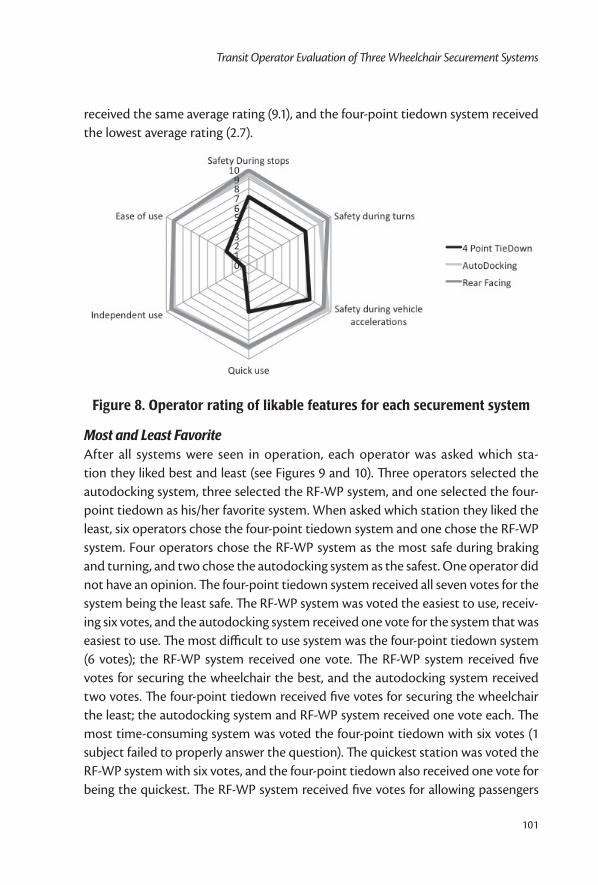
101
Transit Operator Evaluation of Three Wheelchair Securement Systems
received the same average rating (9.1), and the four-point tiedown system received the lowest average rating (2.7).
Figure 8. Operator rating of likable features for each securement system
Most and Least FavoriteAfter all systems were seen in operation, each operator was asked which sta-tion they liked best and least (see Figures 9 and 10). Three operators selected the autodocking system, three selected the RF-WP system, and one selected the four-point tiedown as his/her favorite system. When asked which station they liked the least, six operators chose the four-point tiedown system and one chose the RF-WP system. Four operators chose the RF-WP system as the most safe during braking and turning, and two chose the autodocking system as the safest. One operator did not have an opinion. The four-point tiedown system received all seven votes for the system being the least safe. The RF-WP system was voted the easiest to use, receiv-ing six votes, and the autodocking system received one vote for the system that was easiest to use. The most difficult to use system was the four-point tiedown system (6 votes); the RF-WP system received one vote. The RF-WP system received five votes for securing the wheelchair the best, and the autodocking system received two votes. The four-point tiedown received five votes for securing the wheelchair the least; the autodocking system and RF-WP system received one vote each. The most time-consuming system was voted the four-point tiedown with six votes (1 subject failed to properly answer the question). The quickest station was voted the RF-WP system with six votes, and the four-point tiedown also received one vote for being the quickest. The RF-WP system received five votes for allowing passengers
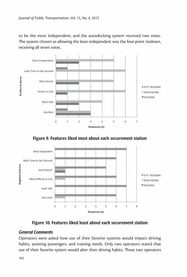
Journal of Public Transportation, Vol. 15, No. 4, 2012
102
to be the most independent, and the autodocking system received two votes. The system chosen as allowing the least independent was the four-point tiedown, receiving all seven votes.
Figure 9. Features liked most about each securement station
Figure 10. Features liked least about each securement station
General CommentsOperators were asked how use of their favorite systems would impact driving habits, assisting passengers, and training needs. Only two operators stated that use of their favorite system would alter their driving habits. These two operators
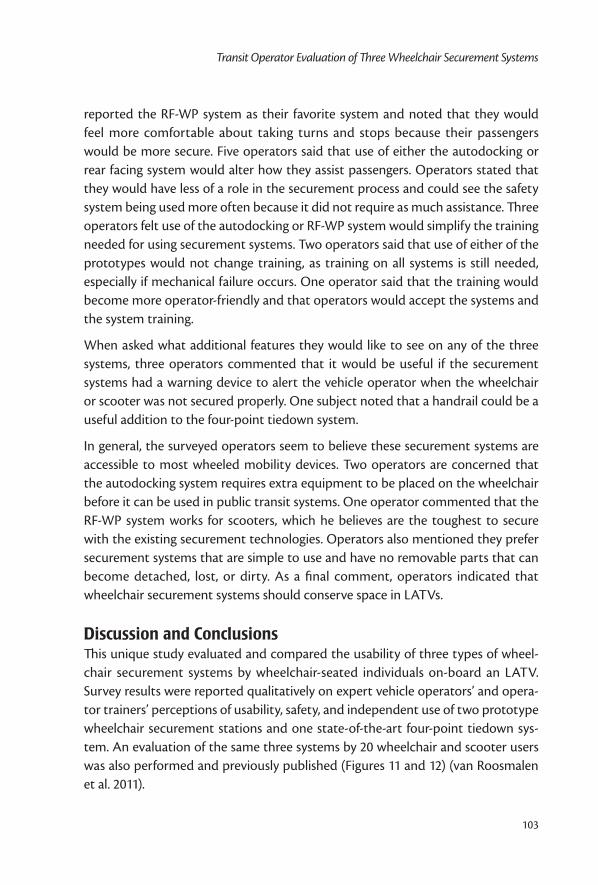
103
Transit Operator Evaluation of Three Wheelchair Securement Systems
reported the RF-WP system as their favorite system and noted that they would feel more comfortable about taking turns and stops because their passengers would be more secure. Five operators said that use of either the autodocking or rear facing system would alter how they assist passengers. Operators stated that they would have less of a role in the securement process and could see the safety system being used more often because it did not require as much assistance. Three operators felt use of the autodocking or RF-WP system would simplify the training needed for using securement systems. Two operators said that use of either of the prototypes would not change training, as training on all systems is still needed, especially if mechanical failure occurs. One operator said that the training would become more operator-friendly and that operators would accept the systems and the system training.
When asked what additional features they would like to see on any of the three systems, three operators commented that it would be useful if the securement systems had a warning device to alert the vehicle operator when the wheelchair or scooter was not secured properly. One subject noted that a handrail could be a useful addition to the four-point tiedown system.
In general, the surveyed operators seem to believe these securement systems are accessible to most wheeled mobility devices. Two operators are concerned that the autodocking system requires extra equipment to be placed on the wheelchair before it can be used in public transit systems. One operator commented that the RF-WP system works for scooters, which he believes are the toughest to secure with the existing securement technologies. Operators also mentioned they prefer securement systems that are simple to use and have no removable parts that can become detached, lost, or dirty. As a final comment, operators indicated that wheelchair securement systems should conserve space in LATVs.
Discussion and ConclusionsThis unique study evaluated and compared the usability of three types of wheel-chair securement systems by wheelchair-seated individuals on-board an LATV. Survey results were reported qualitatively on expert vehicle operators’ and opera-tor trainers’ perceptions of usability, safety, and independent use of two prototype wheelchair securement stations and one state-of-the-art four-point tiedown sys-tem. An evaluation of the same three systems by 20 wheelchair and scooter users was also performed and previously published (Figures 11 and 12) (van Roosmalen et al. 2011).
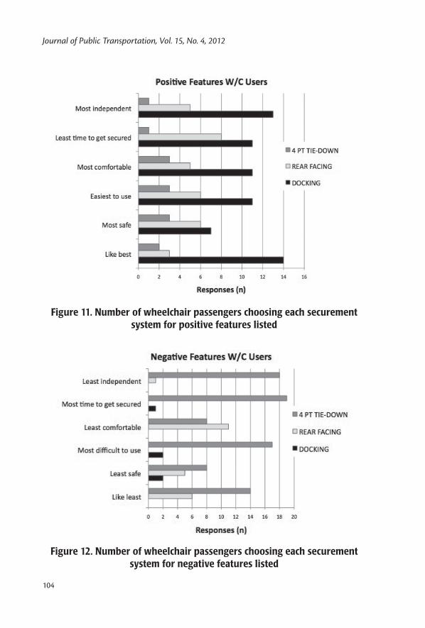
Journal of Public Transportation, Vol. 15, No. 4, 2012
104
Figure 11. Number of wheelchair passengers choosing each securement system for positive features listed
Figure 12. Number of wheelchair passengers choosing each securement system for negative features listed
105
Transit Operator Evaluation of Three Wheelchair Securement Systems
Operators liked the RF-WP system best due to the fact that it does not require operator assistance; it works for scooters; it is quick, secure, and easy to use; and no hardware is needed on wheelchairs for it to work in LATVs. Although also rated highly, the autodocking system raised concern by operators due to the require-ment for wheelchair passengers to align properly and steer backward into the system. While operators prefer the RF-WP system best, wheelchair passengers responded most positively to the autodocking system. According to the wheel-chair passengers surveyed, the RF-WP was favorable due to its perceived stability, ease of use, and security, and because the RF-WP system did not require special wheelchair hardware for it to work on board an LATV. However, about 75 percent of wheelchair passengers mentioned discomfort associated with the use of the RF-WP system, resulting in 30 percent disliking the RF-WP system and 55 percent finding the RF-WP least comfortable to ride in. The discomfort was not only due to riding rearward but also to its perceived contribution to rocking movement induced by vehicle braking and accelerating during rearward travel in the RF-WP system. To improve RF-WP systems, wheelchair passengers suggested a means for upper-body support, improved usability of the system to aid wheelchair passengers in navigating into the system, and an interface that informs wheelchair passengers on upcoming stops. Wheelchair passengers agreed with LATV operators that the autodocking system needs some form of confirmation that the wheelchair is prop-erly aligned and secured in the system.
Operators and wheelchair passengers agreed regarding the four-point tiedown sys-tem. Both liked the four-point tiedown system least due to its lack of independence for wheelchair passengers, its use being time-consuming, its difficulty of use, and the perception of it being less safe and secure than the autodocking and RF-WP systems. Wheelchair passengers suggested redesigning the four-point tiedown sys-tem so that wheelchair users can use the system without operator assistance. They also suggested adding a handhold to the securement station and recommended a better upper-torso restraint to provide more stability.
Public transportation has been attractive to passengers because of its accessible, public nature. Low-floor buses in combination with automated ramps have made a difference in how the increasing number of wheelchair passengers access LATVs. However, current wheelchair securement systems remain designed to require operator assistance. This defeats the purpose of truly accessible transportation and results in misuse and disuse of tiedown systems (Buning et al. 2007; Foreman and Hardin 2001; Frost et al. 2009; Nelson/Nygaard Consulting Associates 2008).
Journal of Public Transportation, Vol. 15, No. 4, 2012
106
For LATVs to be fully accessible, wheelchair securement systems and stations need to be designed accessible to the fullest extent possible. This means that the major-ity of wheelchair and scooter passengers who are able to independently travel can enter the securement station and be independently capable of operating the securement system to secure their wheelchair or scooter. This study supports the need for improvement in securement systems to meet the needs of both LATV operators as well as wheelchair passengers. Future securement systems need to be designed for quick use, the option of forward-facing travel, secure fit, ability to provide feedback to operators and users on correct securement, and usability by the majority of wheelchair passengers. The results from this study will be used to develop novel wheelchair securement systems for use in LATVs.
Acknowledgments
Support for this study was provided by the Department of Education, National Institute on Disability and Rehabilitation Research and the Rehabilitation Engineer-ing Research Center on Wheelchair Transportation Safety (Grant # H133E060064). The opinions expressed herein are from the authors and do not necessarily repre-sent those of the funding agency.
The authors express their thanks to Pittsburgh Port Authority Transit for secure-ment system installation and providing a vehicle and drivers for testing purposes. The authors acknowledge BodyPoint, Q’Straint, Invacare, Amigo, Sunrise Medical, and Sure-Lok for their support with designing prototypes, manufacturing compo-nents, and donating wheelchairs, securement systems, and seat belts.
References
Abelson, J., B. Altom, and D. Cannon. 2008. Status report on the use of wheelchairs and other mobility devices on public and private transportation. San Fran-cisco, California: Easter Seals Project ACTION.
ANSI/RESNA. 2001. ANSI/RESNA WC-19: Wheelchairs used as seats in motor vehi-cles. Arlington: American National Standards Institute (ANSI)/Rehabilitation Engineering Society of North America (RESNA).
Blower, D., L. Schneider, and J. Woodrooffe. 2005. Characterization of transit-bus accidents resulting in passenger injuries for use in developing alternative meth-
107
Transit Operator Evaluation of Three Wheelchair Securement Systems
ods for transporting wheelchair-seated travelers. International Truck & Bus Safety & Security Symposium, November 14–16, 2005, Itasca, IL.
Buning, M. E., C. A. Getchell, G. E. Bertocci, and S. G. Fitzgerald. 2007. Riding a bus while seated in a wheelchair: A pilot study of attitudes and behavior regarding safety practices. Assistive Technology 19(4): 166–179.
Foreman, C., and J. Hardin. 2001. The challenges of wheelchair securement: Search-ing for solutions. Tampa: Center for Urban Transportation Research, National Center for Transit Research, University of South Florida.
Frost, K. L., and G. E. Bertocci. 2009. Retrospective review of adverse incidents involving passengers seated in wheeled mobility devices while traveling in large accessible transit vehicles. Medical Engineering and Physics 32(3): 230–236.
Frost, K. L., and G. Bertocci. 2010. Ingress/egress incidents involving wheelchair users in a fixed-route public transit environment. Public Transportation 13(3): 41–62.
Hardin, J. A., C. C. Foreman, and L. Callejas. 2002. Synthesis of securement device options and strategies. Tampa: National Center for Transit Research (NCTR).
Hobson, D. A., and L. van Roosmalen. 2007. Towards the next generation of wheel-chair securement. Development of a demonstration UDIG-compatible wheel-chair docking device. Assistive Technology 19(4): 210–222.
Hunter-Zaworski, Kate. 2004. An NCAT progress report: Rear facing securement for BRT–A Transit IDEA Project (July 2004). Oregon State University.
International Standards Organization (ISO). 2001. ISO7176, Part 19: Technical sys-tems and aids for disabled or handicapped persons—wheelchairs. Wheeled mobility devices for use in motor vehicles. Geneva, Switzerland: International Standards Organization.
ISO. 2001. ISO/DIS 10542-1: Wheelchair tiedowns and occupant restraint systems—Part 1: Requirements and test methods. Geneva, Switzerland: International Standards Organization.
ISO. 2005. 10542-3: Technical systems and aids for disabled or handicapped per-sons—Wheelchair tiedown and occupant-restraint systems—Part 3: Docking type tiedown systems. Geneva, Switzerland: International Standards Organiza-tion.
Journal of Public Transportation, Vol. 15, No. 4, 2012
108
ISO. 2010. ISO/DIS 10865 Part 1: Assistive products for persons with disability—Wheelchair containment and occupant retention systems for motor vehicles designed for use by both sitting and standing passengers—Part 1: Systems for rearward facing wheelchair-seated passengers. Geneva, Switzerland: Interna-tional Standards Organization.
Nelson/Nygaard Consulting Associates. 2008. Status report on the use of wheel-chairs and other mobility devices on public and private transportation. Wash-ington, D.C: Easter Seals Project ACTION.
Project Action. 2008. Status report on the use of wheelchairs and other mobility devices on public and private transportation. San Francisco, CA.
Shaw, G. 2008. Investigation of large transit vehicle accidents and establishing appropriate protection for wheelchair riders. Journal of Rehabilitation Research and Development 45(1): 85–108.
Society of Automotive Engineers (SAE). 1999. SAE J2249: Wheelchair tiedowns and occupant restraint systems: Surface vehicle recommended practice. Warren-dale, PA: SAE.
Songer, T., S. G. Fitzgerald, and K. Rotko. 2004. The injury risk to wheelchair occu-pants using motor vehicle transportation. 48th Annual Proceedings of the Association for the Advancement of Automotive Medicine.
Turkovich, M. J., L. van Roosmalen, Hobson D. A., and E. A. Porach. 2011. The effect of city bus maneuvers on wheelchair movement. Journal of Public Transporta-tion 14(3): 147–169.
Turkovich, M, J., L. van Roosmalen, D. A. Hobson, and E. A. Porach. 2009. Assess-ment of wheelchair securement systems in a large accessible transit vehicle. Rehabilitation Engineering Society of North America, June, New Orleans.
United Kingdom Department for Transport. 2011. Carriage of mobility scooters on public transport—Feasibility study 2006 [cited March 2 2011]. Available from http://www.dft.gov.uk/transportforyou/access/tipws/cmspt/carriageofmo-bilityscooterson6163.
U. S. Department of Transportation (DOT). 2010. Part 37—Transportation services for individuals with disabilities. 49 CFR 37: Federal Transit Administration.
U. S. DOT. 2010. Part 38—Accessibility specifications for transportation vehicles. 49 CFR 38: Federal Transit Administration.
109
Transit Operator Evaluation of Three Wheelchair Securement Systems
van Roosmalen, L., P. Karg, D. A. Hobson, M. Turkovich, and E. Porach. 2011. User evaluation of wheelchair securement systems in large transit vehicles. Journal of Rehabilitation Research and Development 48(7): 823–838.
About the Authors
Linda van Roosmalen, Ph.D. ([email protected]) is Principal at LINC Design LLC, Verona, PA (www.LINC-Design.com) and lead investigator on the RERC on Wheelchair Transportation Safety.
Douglas A. Hobson, Ph.D. ([email protected]) is Emeritus Associate Profes-sor at the University of Pittsburgh in the Department of Rehabilitation Science and Technology.
Patricia E. Karg, M.S. ([email protected]) is Assistant Professor at the University of Pittsburgh in the Department of Rehabilitation Science and Technology and Co-Director of the RERC on Wheelchair Transportation Safety.
Emily DeLeo, B.S. ([email protected]) is a graduate student at the School of Physical Therapy, Duke University, Durham, NC.
Erik Porach, B.S. ([email protected]) is a Research Specialist at the University of Pittsburgh Department of Rehabilitation Science and Technology. He supports projects in the RERC on Telerehabilitation, Spinal Cord Injury, and on Wheelchair Transportation Safety.

Journal of Public Transportation, Vol. 15, No. 4, 2012
110
Simulated Analysis of Exclusive Bus Lanes on Expressways: Case Study in Beijing, China
111
Simulated Analysis of Exclusive Bus Lanes on Expressways: Case Study in Beijing, China
Lin Zhu, Beijing Jiaotong University Lei Yu, Ph.D., P.E., Texas Southern University
Xu-Mei Chen, Ph.D., Beijing Jiaotong University Ji-Fu Guo, Beijing Transportation Research Center
Abstract
Deploying exclusive bus lanes is considered an important strategy for supporting public transit priority policy. This paper uses a simulation approach to evaluate planned exclusive bus lanes on expressways in Beijing, China. Two scenarios for deploying exclusive bus lanes—a curbside bus lane scenario and a median bus lane scenario—were designed. Then, a micro-simulation network platform using VISSIM was established and calibrated, with all relative errors between the simulated time-varying speeds and the field speeds less than 15 percent. Afterwards, the two bus lane scenarios were simulated, evaluated, and subsequently compared with current traffic conditions without bus lanes. It was found that for both the mainline and the whole network, the operational efficiencies of buses, general traffic, and all mixed traffic are improved with the deployment of exclusive bus lanes. Further, the median bus lane scenario slightly outperforms the curbside bus lane scenario in this case.
IntroductionAs of April 2012, the number of motor vehicles in Beijing, China, was about 5.06 million. The increasing number of vehicles has resulted in many problems, such as traffic congestion, increased emissions, and noise. Improving public traffic is a key
Journal of Public Transportation, Vol. 15, No. 4, 2012
112
strategy for solving traffic problems and has received increased attention from various government agencies in Beijing. Employing exclusive bus lanes is also a basic public transit priority. The basic idea of deploying exclusive bus lanes is to accom-modate large travel demands and improve urban traffic operational efficiency by implementing the proper allocation of space and time resources between buses and general traffic (Yang and Ma 1997). In 1997, Beijing installed its first exclusive bus lane on the right curbside lane of Chang’an Street, which is used only by buses from 6 am to 8 pm. Construction of bus lanes in Beijing is quite slow, and only about 20 bus lanes are built each year. Until now, the total length of exclusive bus lanes was about 303 kilometers in Beijing, which is far from the requests of public transit planning and management. Therefore, in the 12th five-year plan of Beijing, more than 150 exclusive bus lanes will be built.
Expressways are the major arterials in the urban traffic network of Beijing, carry-ing more than 50 percent of the total daily traffic of the city. Traffic conditions on expressways in Beijing indicate that there are extremely high traffic volumes, a high density of public transit lines, large bus flows at bus stops, and high densities at on- and off-ramps. A commonly-observed phenomenon is that, to get through the already-congested roads, automobiles and buses must compete for the right-of-way without concessions, resulting in even worse traffic conditions. Therefore, relevant agencies are proposing to deploy exclusive bus lanes on expressways to reduce conflicts between vehicles by physically separating automobiles and buses. However, exclusive bus lanes are usually constructed on urban arterials and other key roads of general grades, and employing exclusive bus lanes on expressways is less common.
There is no doubt that exclusive bus lanes will have some degree of impact on road traffic, which has been studied by a number of researchers. Based on simulations and field surveys, St. Jacques and Levinson (1997) developed an analysis procedure for estimating capacities and speeds on arterials with at least one exclusive bus lane with either no, partial, or exclusive use of the adjacent lane. Siddique and Khan (2006) used NETSIM to model and forecast traffic conditions along BRT corridors in Ottawa for 2021, which were compared with traffic conditions in 2001. The study focused on the capacity analysis of BRT operation on exclusive bus lanes.
Although the deployment of exclusive bus lanes on expressways has been planned, relevant studies are still rare. Chen et al. (2009) analyzed the impacts of exclusive bus lanes on the capacity of the ring-road expressway using the VISSIM model. The analyzed parameters included the styles and distances of ramps, length of weaving
Simulated Analysis of Exclusive Bus Lanes on Expressways: Case Study in Beijing, China
113
sections, bus headway, and others. The simulation results showed that weaving sec-tion length and bus headway are more sensitive, especially for on- and off-ramps for curbside bus lanes.
In light of the above, the research in this paper simulated the impact of deploying exclusive bus lanes on an expressway. To this end, it first carried out a series of com-prehensive traffic surveys and data collections along the Western 3rd Ring-Road Expressway in Beijing. Second, it explained the conditions of setting an exclusive bus lane and designed two bus lane scenarios, including a median bus lane and a curbside bus lane. Then, it established a simulation platform using VISSIM for the Western 3rd Ring-Road Expressway and calibrated the model parameters. Finally, it comparatively simulated and evaluated the two designed scenarios of an exclusive bus lane.
Study Area and Data CollectionDescription of Western 3rd Ring-Road ExpresswayExisting ring-road expressways in Beijing include the 2nd, 3rd, 4th, 5th, and 6th ring-road expressways. The selected network in this study is the main portion of the Western 3rd Ring-Road Expressway Network, which is about 8.5 kilometers long in the south-north direction, including 7 interchange bridges, as shown in Figure 1. The Western 3rd Ring-Road Expressway provides 3 lanes in each direction with widths of 3.5 meters, 3.25 meters, and 3.5 meters for median, center, and shoulder lanes, respectively, as well as an emergency lane that is 4.75 meters wide. There are frontage roads present with two lanes in each direction along the expressway, which are connected to the mainline through ramps. A green zone with a width of 2 meters is reserved in the middle of two directions as well as between the mainline and frontage roads.
One of the busiest traffic corridors in Beijing, the Western 3rd Ring-Road Express-way is crossed by four urban expressways and four major arterials. Along and near the expressway, there exist Lize Bridge Coach Station, Liuli Bridge Coach Station, Lianghuachi Coach Station, and Beijing Western Railway Station, the largest railway station in Beijing. Public transit demand is quite high in this area, with a total of more than 40,000 passengers per day getting on and off buses at each bus stop. The bus cross-sectional volume in the peak hours reaches 300 vehicles per hour, including 12- or 14-meter single buses; articulated buses 14, 16 or 18 meters in length; and 10- or 12-meter double-deck buses. Thus, many large vehicles run on
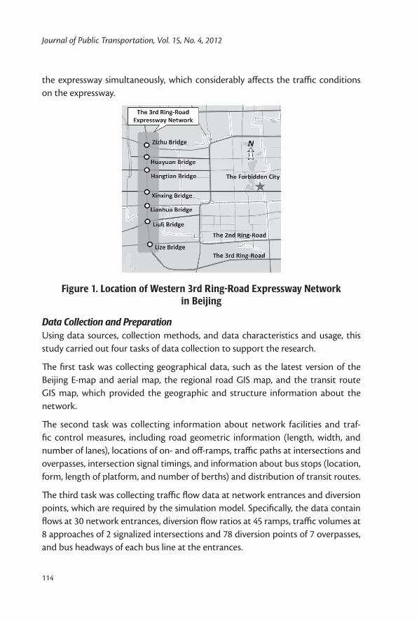
Journal of Public Transportation, Vol. 15, No. 4, 2012
114
the expressway simultaneously, which considerably affects the traffic conditions on the expressway.
Figure 1. Location of Western 3rd Ring-Road Expressway Network in Beijing
Data Collection and PreparationUsing data sources, collection methods, and data characteristics and usage, this study carried out four tasks of data collection to support the research.
The first task was collecting geographical data, such as the latest version of the Beijing E-map and aerial map, the regional road GIS map, and the transit route GIS map, which provided the geographic and structure information about the network.
The second task was collecting information about network facilities and traf-fic control measures, including road geometric information (length, width, and number of lanes), locations of on- and off-ramps, traffic paths at intersections and overpasses, intersection signal timings, and information about bus stops (location, form, length of platform, and number of berths) and distribution of transit routes.
The third task was collecting traffic flow data at network entrances and diversion points, which are required by the simulation model. Specifically, the data contain flows at 30 network entrances, diversion flow ratios at 45 ramps, traffic volumes at 8 approaches of 2 signalized intersections and 78 diversion points of 7 overpasses, and bus headways of each bus line at the entrances.
Simulated Analysis of Exclusive Bus Lanes on Expressways: Case Study in Beijing, China
115
The final part task collecting data from Remote Traffic Microwave Sensors (RTMS) and the transit data from Global Position System (GPS). RTMS data can provide flow and speed information at 20 sections along the Western 3rd Ring-Road Expressway. The original data collected at 2-minute intervals by RTMS were aggre-gated into data at time intervals of 10 minutes, 1 hour, or 2 hours. In the study, hand-carried GPS units were used to collect bus speed data at 2-second intervals for selected bus lines by boarding on buses. These data were used in the calibration and validation of the simulation model.
Design of Exclusive Bus Lanes on ExpresswaysConditions of Setting an Exclusive Bus Lane This section explains the conditions of setting an exclusive bus lane, as follows:
(1) Geometric conditions on the road: There should be at least 2 lanes in each direction on the road, and it is better if there are 3 or 4 lanes (Lu 2003). Considering the needed space for bus vehicles, the width of a bus lane usu-ally equals 3.5 meters, which can be appropriately reduced but should be at least 3 meters (Yang 2003). The Western 3rd Ring-Road Expressway has 3 lanes in each direction with widths of 3.5 meters, 3.25 meters, and 3.5 meter, respectively, and an emergency lane that is 4.75 meters wide. Accordingly, the geometric structure of the Western 3rd Ring-Road Expressway meets the physical requirements of deploying exclusive bus lanes.
(2) Traffic saturation level on the road: It is necessary to deploy an exclusive bus lane when the volume-to-capacity ratio on a road arrives at or exceeds the value of 0.8 (Zhang et al. 2000). According to the surveyed flow data, the average volume-to-capacity ratio on the Western 3rd Ring-Road Express-way is 0.94, and the values of several sections are higher than 1.
(3) Bus volume on the road section: It is suggested to build an exclusive bus lane if bus volume on a road section in peak hours is higher than 150 vehicles per hour (Yang et al. 2000). The field surveyed data indicate that the bus volume in the peak hours on the mainline of the Western 3rd Ring-Road Expressway is more than 225 vehicles per hour.
(4) Public transit passenger volume on the road section: The Highway Capacity Manual (National Research Council 2000) suggests that passenger volume on a bus lane should be 50 percent higher than that on other lanes, and this value should be more than 3,000 person-trips per hour on the planned
Journal of Public Transportation, Vol. 15, No. 4, 2012
116
bus lane in Shanghai (Lin et al. 2007). According to the surveyed data, the average passenger volume of public transit on the Western 3rd Ring-Road Expressway is about 17,750 person-trips per hour in the peak hours and occupies about 70 percent of total service passenger volume on the section.
Consequently, it is qualified and necessary to deploy an exclusive bus lane on the Western 3rd Ring-Road Expressway in Beijing.
Scenario Designs of Exclusive Bus LaneThe key elements in the design of exclusive bus lanes on expressways include physi-cal location of the bus lane, structure of the bus stops, ramp control towards buses, and corresponding adjustment of bus lines, all of which have been considered in the designs of the two exclusive bus lane scenarios on the Western 3rd Ring-Road Expressway. Basic on the current structure of the roads, two exclusive bus lane scenarios were designed (as shown in Figure 2), which were modeled and evaluated with the established VISSIM simulation model.
Basic ScenarioCurrent traffic conditions without the exclusive bus lane were simulated based on the field data collected.
Scenario 1: Curbside Bus Lane Scenario
With the road structure of the mainline unchanged, a curbside lane was used as the bus lane in this scenario. There were no major structural and positional changes on bus stops, i.e., bus bays remained the same, passenger waiting areas continued to occupy the green zone, and buses parked in the emergency lane, as shown in Figure 2. Buses ran on the curbside lane and could enter or exit the bus lane conveniently. All buses followed the current routes.
Scenario 2: Median Bus Lane Scenario
In this scenario, the median lane was used as the bus lane. Therefore, bus stops were moved from the curbside to the center of the expressway. The widths of the general traffic lanes and the emergency lane were slightly narrowed to ensure adequate space required for parking the buses. Figure 2 shows the configuration of the bus stop area in the median bus lane scenario. Buses had to enter or exit the median bus lane by crossing two general traffic lanes, which caused a serious interference with traffic. Therefore, a bus ramp control strategy was proposed, which meant that when running in the median bus lane, buses could enter the mainline only from one on-ramp and exit the mainline only from one off-ramp. In this design, bus
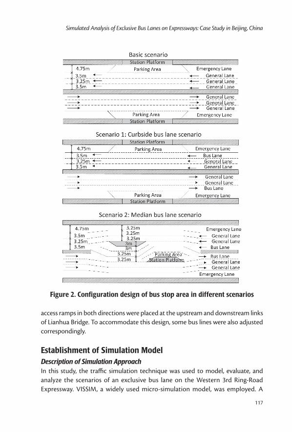
Simulated Analysis of Exclusive Bus Lanes on Expressways: Case Study in Beijing, China
117
Figure 2. Configuration design of bus stop area in different scenarios
access ramps in both directions were placed at the upstream and downstream links of Lianhua Bridge. To accommodate this design, some bus lines were also adjusted correspondingly.
Establishment of Simulation ModelDescription of Simulation ApproachIn this study, the traffic simulation technique was used to model, evaluate, and analyze the scenarios of an exclusive bus lane on the Western 3rd Ring-Road Expressway. VISSIM, a widely used micro-simulation model, was employed. A
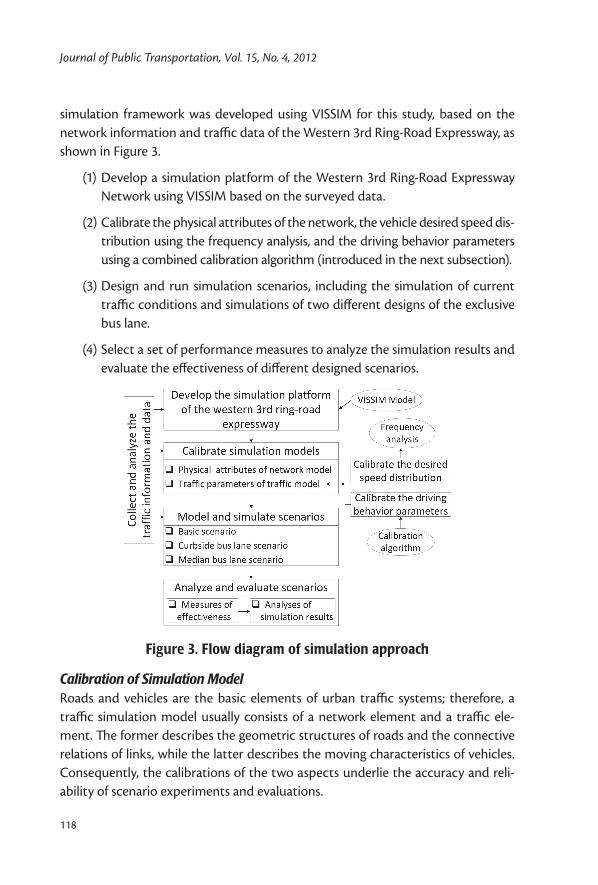
Journal of Public Transportation, Vol. 15, No. 4, 2012
118
simulation framework was developed using VISSIM for this study, based on the network information and traffic data of the Western 3rd Ring-Road Expressway, as shown in Figure 3.
(1) Develop a simulation platform of the Western 3rd Ring-Road Expressway Network using VISSIM based on the surveyed data.
(2) Calibrate the physical attributes of the network, the vehicle desired speed dis-tribution using the frequency analysis, and the driving behavior parameters using a combined calibration algorithm (introduced in the next subsection).
(3) Design and run simulation scenarios, including the simulation of current traffic conditions and simulations of two different designs of the exclusive bus lane.
(4) Select a set of performance measures to analyze the simulation results and evaluate the effectiveness of different designed scenarios.
Figure 3. Flow diagram of simulation approach
Calibration of Simulation ModelRoads and vehicles are the basic elements of urban traffic systems; therefore, a traffic simulation model usually consists of a network element and a traffic ele-ment. The former describes the geometric structures of roads and the connective relations of links, while the latter describes the moving characteristics of vehicles. Consequently, the calibrations of the two aspects underlie the accuracy and reli-ability of scenario experiments and evaluations.
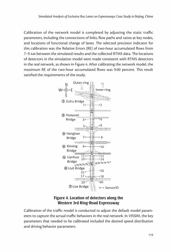
Simulated Analysis of Exclusive Bus Lanes on Expressways: Case Study in Beijing, China
119
Calibration of the network model is completed by adjusting the static traffic parameters, including the connections of links, flow paths and ratios at key nodes, and locations of functional change of lanes. The selected precision indicator for this calibration was the Relative Errors (RE) of two-hour accumulated flows from 7–9 am between the simulated results and the collected RTMS data. The locations of detectors in the simulation model were made consistent with RTMS detectors in the real network, as shown in Figure 4. After calibrating the network model, the maximum RE of the two-hour accumulated flows was 9.00 percent. This result satisfied the requirements of the study.
Figure 4. Location of detectors along the Western 3rd Ring-Road Expressway
Calibration of the traffic model is conducted to adjust the default model param-eters to capture the actual traffic behaviors in the real network. In VISSIM, the key parameters that needed to be calibrated included the desired speed distribution and driving behavior parameters.
Journal of Public Transportation, Vol. 15, No. 4, 2012
120
In VISSIM, desired speed distribution is defined to describe the fact that a driver will travel at a desired speed (with a stochastic variation) when not hindered by other vehicles. The maximum and minimum values for the desired speed, as well as the intermediate points, are determined by a frequency analysis of the vehicle speed data collected during free-flow periods. The desired speed distribution of general traffic was obtained by analyzing the speed data from RTMS on the West-ern 3rd Ring-Road Expressway from 12–6 am on October 7 and 8, 2008; the desired speed distribution of buses on general lanes was obtained by analyzing the GPS speed data of buses on the Western 3rd Ring-Road Expressway from 2–4 pm (the lowest bus-flow period). It was noted that there are no deployed bus lanes on the Western 3rd Ring-Road Expressway at present. Therefore, the GPS speed data of buses on the section from Xizhimen Bridge to Jishuitan Bridge of the 2nd ring-road from 7–9 am were collected and analyzed to obtain the desired speed distribution of buses on the bus lane and represent the bus running condition on the bus lane on the Western 3rd Ring-Road Expressway.
In VISSIM, driving behavior parameters describe the vehicle-following and lane-changing behaviors, lateral behavior, and reaction behavior to signals. In a sensitiv-ity analysis of parameters using a simple network, 10 driving behavior parameters were screened, including the maximum look-ahead distance, average standstill distance, additive part of safety distance, multiplicable part of safety distance, maximum deceleration for lane changes, accepted deceleration for lane changes, waiting time before diffusion, minimum headway for lane changes, reduction rate (as meters per 1 m/s²), and minimum lateral distance for 50 km/h. Combining the Generic Algorithm (GA) with the Simultaneous Perturbation Stochastic Approxi-mation Algorithm (SPSA), a calibration program for driving behavior parameters was developed using Visual C++ and MATLAB languages. First, the parameters were locked in a relatively small area using the GA, overcoming the SPSA’s short-coming of inefficient global optimization; then, the SPSA was used to solve the problem in the locked area, overcoming the slow convergence of GA. In the calibra-tion process, the Sum of Squared Error (SSE) between the simulated time-varying speeds and the actual speeds was selected as the measure to determine the best combination of the 10 parameters for the Western 3rd Ring-Road Expressway sim-ulation model. The calibration algorithm is explained in detail by Chen et al. (2011).
After completing the calibrations of network model and traffic model, the time-varying speeds at 10-minute intervals were output from 20 detectors, and then the simulation results were compared with the RTMS data. The simulated time-varying
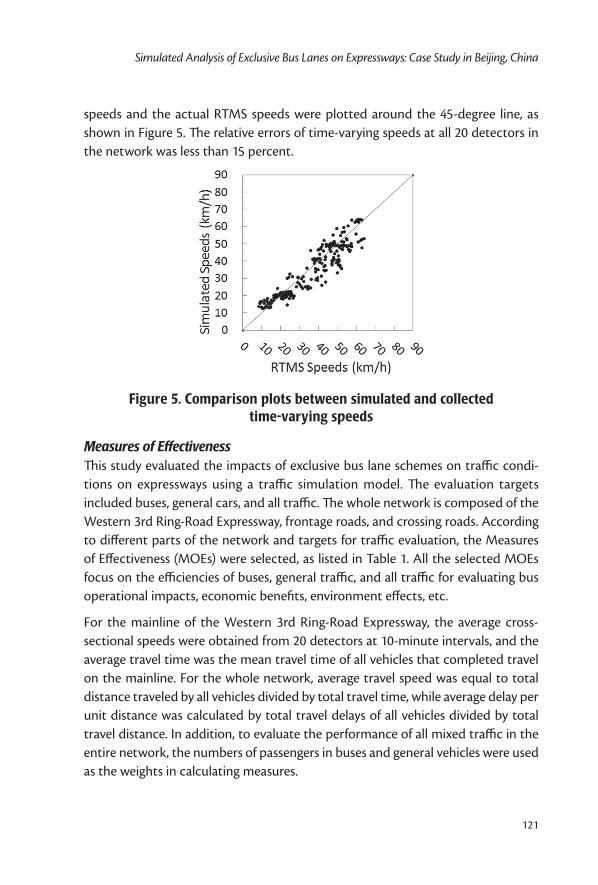
Simulated Analysis of Exclusive Bus Lanes on Expressways: Case Study in Beijing, China
121
speeds and the actual RTMS speeds were plotted around the 45-degree line, as shown in Figure 5. The relative errors of time-varying speeds at all 20 detectors in the network was less than 15 percent.
Figure 5. Comparison plots between simulated and collected time-varying speeds
Measures of EffectivenessThis study evaluated the impacts of exclusive bus lane schemes on traffic condi-tions on expressways using a traffic simulation model. The evaluation targets included buses, general cars, and all traffic. The whole network is composed of the Western 3rd Ring-Road Expressway, frontage roads, and crossing roads. According to different parts of the network and targets for traffic evaluation, the Measures of Effectiveness (MOEs) were selected, as listed in Table 1. All the selected MOEs focus on the efficiencies of buses, general traffic, and all traffic for evaluating bus operational impacts, economic benefits, environment effects, etc.
For the mainline of the Western 3rd Ring-Road Expressway, the average cross-sectional speeds were obtained from 20 detectors at 10-minute intervals, and the average travel time was the mean travel time of all vehicles that completed travel on the mainline. For the whole network, average travel speed was equal to total distance traveled by all vehicles divided by total travel time, while average delay per unit distance was calculated by total travel delays of all vehicles divided by total travel distance. In addition, to evaluate the performance of all mixed traffic in the entire network, the numbers of passengers in buses and general vehicles were used as the weights in calculating measures.
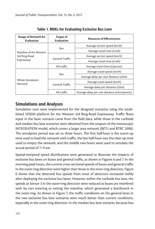
Journal of Public Transportation, Vol. 15, No. 4, 2012
122
Table 1. MOEs for Evaluating Exclusive Bus Lane
Range of Network for Evaluation
Target of Evaluation
Measures of Effectiveness
Mainline of the Western 3rd Ring-Road Expressway
BusAverage section speed (km/h)
Average travel time (s/veh)
General TrafficAverage section speed (km/h)
Average travel time (s/veh)
All traffic Average travel time (s/person)
Whole Simulation Network
BusAverage travel speed (km/h)
Average delay per unit distance (s/km)
General TrafficAverage travel speed (km/h)
Average delay per distance (s/km)
All traffic Average delay per unit distance (s/km/person)
Simulations and AnalysesSimulation runs were implemented for the designed scenarios using the estab-lished VISSIM platform for the Western 3rd Ring-Road Expressway. Traffic flows input in the basic scenario came from the field data, while those in the curbside and median bus lane scenarios were obtained from the outputs of the mesoscopic INTEGRATION model, which covers a larger area network (BJTU and BTRC 2008). The simulation period was set to three hours. The first half-hour is the warm-up time used to load the network with traffic, the last half-hour was the clear-up time used to empty the network, and the middle two hours were used to simulate the actual period of 7–9 am.
Spatial-temporal speed distributions were generated to illustrate the impacts of exclusive bus lanes on buses and general traffic, as shown in Figures 6 and 7. In the morning peak hours, the current cross-sectional speeds of buses and general traffic in the outer-ring direction were higher than those in the inner-ring direction. Figure 6 shows that the detected bus speeds from most of detectors increased visibly after deploying the exclusive bus lanes. However, within the curbside bus lane, the speeds at Sensor 3 in the outer-ring direction were reduced as buses are interfered with by cars entering or exiting the mainline, which generated a bottleneck in the outer-ring. As shown in Figure 7, the traffic conditions on the general lanes in the two exclusive bus lane scenarios were much better than current conditions, especially in the outer-ring direction. In the median bus lane scenario, because bus
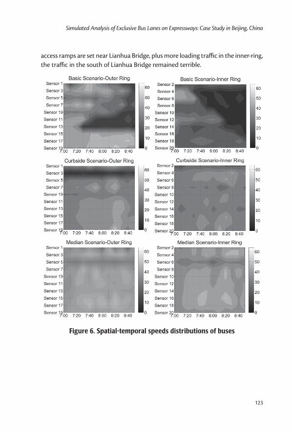
Simulated Analysis of Exclusive Bus Lanes on Expressways: Case Study in Beijing, China
123
access ramps are set near Lianhua Bridge, plus more loading traffic in the inner-ring, the traffic in the south of Lianhua Bridge remained terrible.
Figure 6. Spatial-temporal speeds distributions of buses
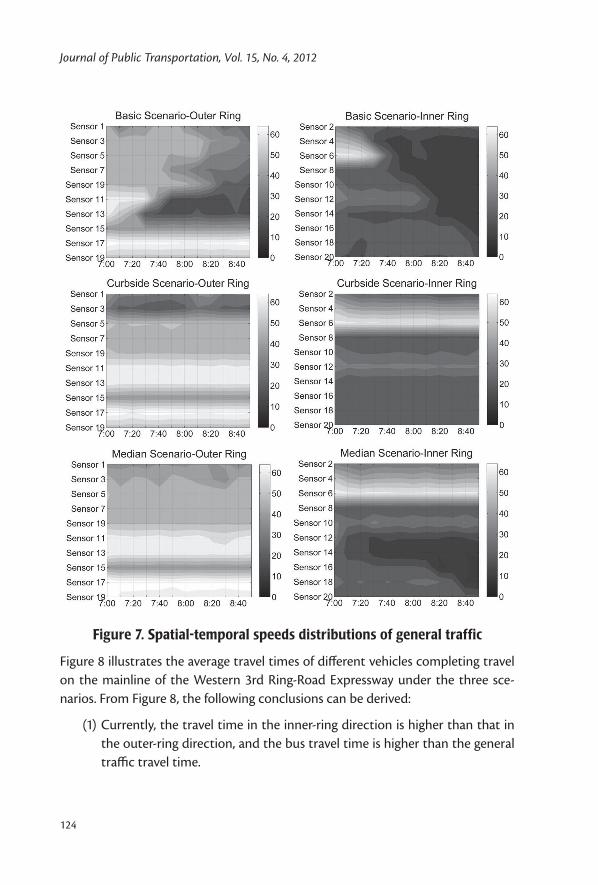
Journal of Public Transportation, Vol. 15, No. 4, 2012
124
Figure 7. Spatial-temporal speeds distributions of general traffic
Figure 8 illustrates the average travel times of different vehicles completing travel on the mainline of the Western 3rd Ring-Road Expressway under the three sce-narios. From Figure 8, the following conclusions can be derived:
(1) Currently, the travel time in the inner-ring direction is higher than that in the outer-ring direction, and the bus travel time is higher than the general traffic travel time.
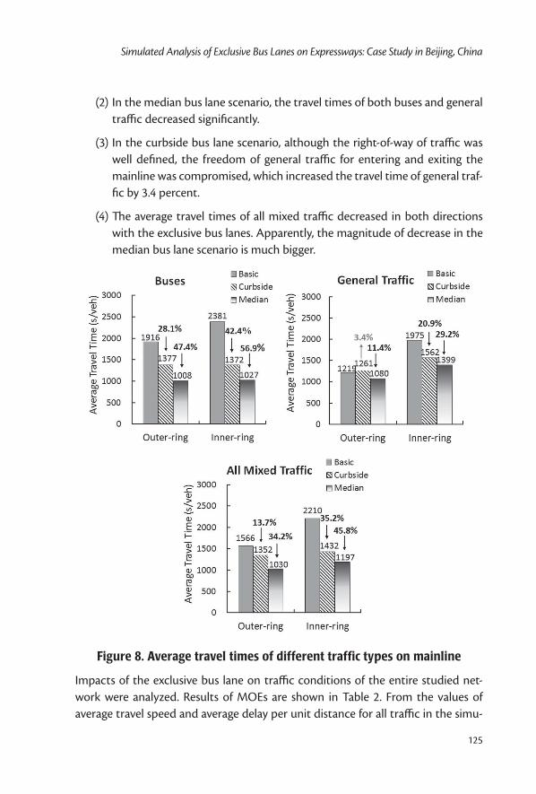
Simulated Analysis of Exclusive Bus Lanes on Expressways: Case Study in Beijing, China
125
(2) In the median bus lane scenario, the travel times of both buses and general traffic decreased significantly.
(3) In the curbside bus lane scenario, although the right-of-way of traffic was well defined, the freedom of general traffic for entering and exiting the mainline was compromised, which increased the travel time of general traf-fic by 3.4 percent.
(4) The average travel times of all mixed traffic decreased in both directions with the exclusive bus lanes. Apparently, the magnitude of decrease in the median bus lane scenario is much bigger.
Figure 8. Average travel times of different traffic types on mainline
Impacts of the exclusive bus lane on traffic conditions of the entire studied net-work were analyzed. Results of MOEs are shown in Table 2. From the values of average travel speed and average delay per unit distance for all traffic in the simu-
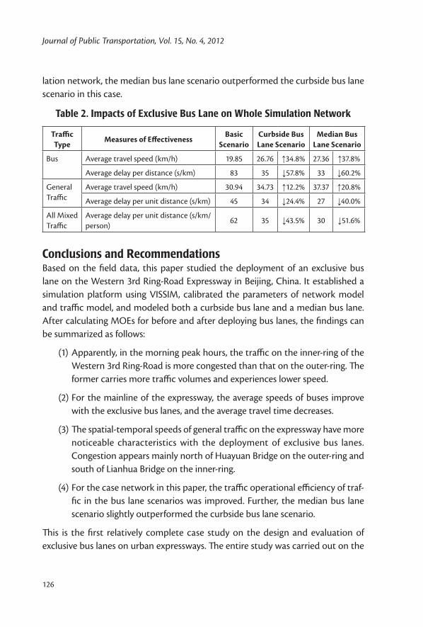
Journal of Public Transportation, Vol. 15, No. 4, 2012
126
lation network, the median bus lane scenario outperformed the curbside bus lane scenario in this case.
Table 2. Impacts of Exclusive Bus Lane on Whole Simulation Network
Traffic Type
Measures of EffectivenessBasic
ScenarioCurbside Bus Lane Scenario
Median Bus Lane Scenario
Bus Average travel speed (km/h) 19.85 26.76 ↑34.8% 27.36 ↑37.8%
Average delay per distance (s/km) 83 35 ↓57.8% 33 ↓60.2%
General Traffic
Average travel speed (km/h) 30.94 34.73 ↑12.2% 37.37 ↑20.8%
Average delay per unit distance (s/km) 45 34 ↓24.4% 27 ↓40.0%
All Mixed Traffic
Average delay per unit distance (s/km/person)
62 35 ↓43.5% 30 ↓51.6%
Conclusions and RecommendationsBased on the field data, this paper studied the deployment of an exclusive bus lane on the Western 3rd Ring-Road Expressway in Beijing, China. It established a simulation platform using VISSIM, calibrated the parameters of network model and traffic model, and modeled both a curbside bus lane and a median bus lane. After calculating MOEs for before and after deploying bus lanes, the findings can be summarized as follows:
(1) Apparently, in the morning peak hours, the traffic on the inner-ring of the Western 3rd Ring-Road is more congested than that on the outer-ring. The former carries more traffic volumes and experiences lower speed.
(2) For the mainline of the expressway, the average speeds of buses improve with the exclusive bus lanes, and the average travel time decreases.
(3) The spatial-temporal speeds of general traffic on the expressway have more noticeable characteristics with the deployment of exclusive bus lanes. Congestion appears mainly north of Huayuan Bridge on the outer-ring and south of Lianhua Bridge on the inner-ring.
(4) For the case network in this paper, the traffic operational efficiency of traf-fic in the bus lane scenarios was improved. Further, the median bus lane scenario slightly outperformed the curbside bus lane scenario.
This is the first relatively complete case study on the design and evaluation of exclusive bus lanes on urban expressways. The entire study was carried out on the
Simulated Analysis of Exclusive Bus Lanes on Expressways: Case Study in Beijing, China
127
basis of comprehensive and extensive field traffic data. Therefore, the study results are of practically significance.
Evaluations in the paper, which focus mainly on traffic impacts, are still quite gen-eral. It is recommended that further studies be conducted on the special traffic operational problems associated with the deployment of exclusive bus lanes, such as impacts on the traffic near bus stops, traffic conditions near on- and off-ramps, etc. This paper focuses only on the corridor network of the Western 3rd Ring-Road Expressway. It is, therefore, recommended that the study be expanded in the future to other networks with different locations and scopes, such as the other ring-road expressways or radial roads.
Acknowledgment
This paper was prepared based on support from Major Projects of the Beijing Transportation Research Center #T08L04404 and #CZ200704 and from Funda-mental Research Funds for the Central Universities #2009YJS045.
References
Beijing Jiaotong University (BJTU) and Beijing Transportation Research Center (BTRC). 2008. The Research Report of Dynamic Traffic Model for Beijing. Beijing, China.
Chen X. M., L. Yu, L. Zhu, J. F. Guo, and M. Z. Sun. 2009. Capacity analysis of weaving sections on an urban expressway with exclusive bus lanes using microscopic traffic simulation. 88th Transportation Research Board Annual Meeting CD-ROM, #09-0535, Washington, D.C.
Chen X. M., L. Yu, L. Y. Zhu, Y. Zhang, and Z. Lin. 2011. Calibrating and validating a micro-simulation model of a bus rapid transit corridor with heuristic optimiza-tion methods. 90th Transportation Research Board Annual Meeting CD-ROM, #11-2641, Washington, D.C.
Lin T., K. F. Yang, and J. X. Zheng. 2007. Study on bus lane system planning method: Case study of Shenzhen. Traffic & Transportation 7: 1–4.
Lu J. 2003. Study of installation conditions of bus lanes. Communications Standard-ization 1: 59–61.
Journal of Public Transportation, Vol. 15, No. 4, 2012
128
National Research Council. 2000. Highway Capacity Manual 2000. Washington, D.C.: Transportation Research Board.
Siddique, A. J., and A. M. Khan. 2006. Microscopic simulation approach to capac-ity analysis of bus rapid transit corridors. Journal of Public Transportation 9: 181–200.
St. Jacques, K., and H. S. Levinson. 1997. Operational analysis of bus lanes on arte-rials. TCRP A-7. Washington, D.C.: Transportation Research Board, National Research Council.
Yang, X. G., and L. Ma. 1997. Design features and priority control and management on urban bus lanes. City Planning Review 3: 36–37.
Yang, X. G., G. W. Zhou, M. S. Hang, and C. H. Shi. 2000. Technologies and methods of transit priority. Urban Transport of China 2: 1–12.
Yang, X. G. 2003. Manual of Urban Traffic Design. Beijing: China Communications Press.
Zhang, W. H., Y. J. Huang, and G. Hu. 2003. Study on design standards for urban bus lanes. Communications Standardization 7: 33–36.
About the Authors
Lin Zhu ([email protected]) is a Ph.D. Candidate at School of Traffic and Transportation, Beijing Jiaotong University, Beijing, China. Her research interests involve public transit planning and management, transportation simulation, and Intelligent Transportation Systems.
Lei Yu, Ph.D., P.E. ([email protected]) is Professor and Dean of the College of Science and Technology, Texas Southern University, and a Yangtze River Scholar of Beijing Jiaotong University. He has managed more than 80 research projects and published more than 200 scientific papers.
Xu-Mei Chen, Ph.D. ([email protected]) is Associate Professor at the School of Traf-fic and Transportation, Beijing Jiaotong University, Beijing, China. Her researches interests involve ITS technologies, urban traffic planning and management, public transit operation, and industry policy of transportation.
Ji-Fu Guo, Ph.D. ([email protected]) is Director of Beijing Transportation Research Center. His main research areas involve traffic forecasting, metro/highway planning, traffic impact analysis, traffic simulation, and traffic environment analysis.