journal of technical analysis (jota). issue 07 (1980, february)

Market Technicians Association

JOURNAL Issue 7 February 1980

MARKET TECHNICIANS ASSOCIATiON JOURNAL

Issue 7

February, 1980

Published by: Market Technicians Association 70 Pine Street

New York, New York 10005

Copyright 1980 by Market Technicians Association

intentionally blank

2

Market Technicians Association Journal

Editor: William DiIanni, V.P. Wellington Management Co. 28 State Street Boston, Massachusetts 02109

Associate Editor: Cheryl Stafford Wellington Management Co.

Editorial Advisor: William S. Doane Fidelity Management & Research

Thanks to the following MTA members and subscribers for their part in the creation of this issue:

Bernard Fremerman Charles D. Kirkpatrick II Arthur A. Merrill Richard C. Orr Henry 0. Pruden, Ph.D. Stan Weinstein

3

MARKET TECHNICIANS ASSOCIATION MEMBERSHIP and SUBSCRIPTION INFORMATION

REGULAR MEMBERSHIP - $50 per year plus $10 one-time application fee.

Receives the Journal, the monthly MTA Newsletter, invitations to all meetings, voting member status and a discount on the Annual Seminar Fee. Eligibility requires that the emphasis of the applicant's professional work involve technical analysis.

SUBSCRIBER STATUS - $50 per year plus $10 one-time application fee.

Receives the Journal and the MTA Newsletter, which contains shorter articles on technical analysis, and the subscriber receives special announcements of the MTA meetings open to The New York Society of Security Analysts and/or the public, plus a discount on the Annual Seminar Fee.

ANNUAL SUBSCRIPTION TO THE MTA JOURNAL - $35 per year.

SINGLE ISSUES OF THE MTA JOURNAL (including back issues)

are available for $10 to regular members or subscribers $15 to non-members and non-subscribers

The Market Technicians Association Journal is scheduled to be published three times each fiscal year, in approximately November, February and May.

An Annual Seminar is held each spring.

Inquiries for Membership should be directed to:

Fred R. Gruber, V.P. United Jersey Bank 210 Main Street Hackensack, New Jersey 07602

4

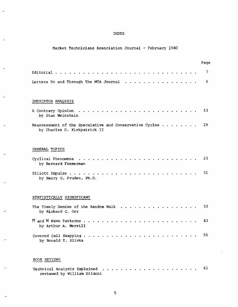
INDEX

Market Technicians Association Journal - February 1980

Page

Editorial............................... 7

Letters To and Through The MTA Journal . . . . . . . . . . . . . . . . 9

INDICATOR ANALYSIS

A Contrary Opinion . . . . . . . . . . . . . . . . . . . . . . . . . . 13 by Stan Weinstein

Reassessment of the Speculative and Conservative Cycles . . . . . . . . 19 by Charles D. Kirkpatrick II

GENERAL TOPICS

Cyclical Phenomena . . . . . . . . . . . . . . . . . . . . . . . . . . 23 by Bernard Fremerman

Elliott Impulse . . . . . . . . . . . . . . . . . . . . . . . . . . . . 31 by Henry 0. Pruden, Ph.D.

STATISTICALLY SIGNIFICANT

The Timely Demise of the Random Walk . . . . . . . . . . . . . . . . . 33 by Richard C. Orr

M and Wwave Patterns. . . . . . . . . . . . . . . . . . . . . . . . . 43 by Arthur A. Merrill

Covered Call Swapping . . . . . . . . . . . . . . . . . . . . . . . . . 55 by Ronald T. Slivka

BOOK REVIEWS

Technical Analysis Explained . . . . . . . . . . . . . . . . . . . . . 61 reviewed by William DiIanni

5

intentionally blank

6

EDITORIAL: ON WRITING AND CRITICISM

One must be impressed with the quantity and quality of books being published on a subject matter close to the hearts of all of us; namely, "Elliott Wave Principle" by Frost and Prechter, "Technical Analysis Explained" by Marty Pring, "Cycles" by Dick Stoken, "Buy Low, Sell High" by John Mahoney, "Stock Market Strategy" by Richard Crowell, just to name a few.

The work, the depth, the quality shines through as the proverbial beacon in the night encouraging others to follow. Undoubtedly, many others will be inspired by their efforts to bring out new ideas and update old ones. There is a trend beginning here that should be encouraged and exploited via the published book process and via the articles written for the Market Technicians Association Journal.

We were likewise gratified by the response the staff received for the last issue of the Journal. The issue was praised both on the matter of format and the matter of content. And since content is more important, we wish to thank all who contributed of their time and talent . . . both are precious.

I sense there is another trend emerging, however, that is a bit distrubing. And that is "ad hominem" criticism that creeps up from time to time in public talks and other forms of writing. It is understandable that over a beer with a few close friends, one can accentuate an opinion by saying: "Yes, I read his last market letter and the so-and-so is an idiot!" . . . (or some other denigrating verbiage). What should be frowned upon is the

use of some such statement in writings or public addresses. We can surely assume these "ad hominem" attacks are to be taken in good fun, but they could get out of hand and are clearly not in good taste.

If an organization such as the Market Technicians Association is to main- tain high standards of quality, one should not allow such behaviour to go too far. For the level of any organization is also judged by the behaviour level of its members or guests. And "ad hominem" attacks are the lowest form of criticism, the least dignified . . . levelled at the man, not the material.

But proper criticism has its place and can be helpful for all involved. As Francis Mauriac said: II . . . Certainly the writer despises these criti- cisms, but he cannot prevent himself from thinking about them a great deal: because even if the conclusions of so-and-so appear to him unjust and crude, he cannot say the same of the premises. Thus he is bound to be led back to his own profound interior contradictions. The silliest article has this in its favor: that it obliges the author to face up to this problem, and we should not ask more of our judges than to be led back to confront our own difficulties."

Three cheers for writing, criticism and good taste!

William DiIanni, Editor February, 1980

intentionally blank

8

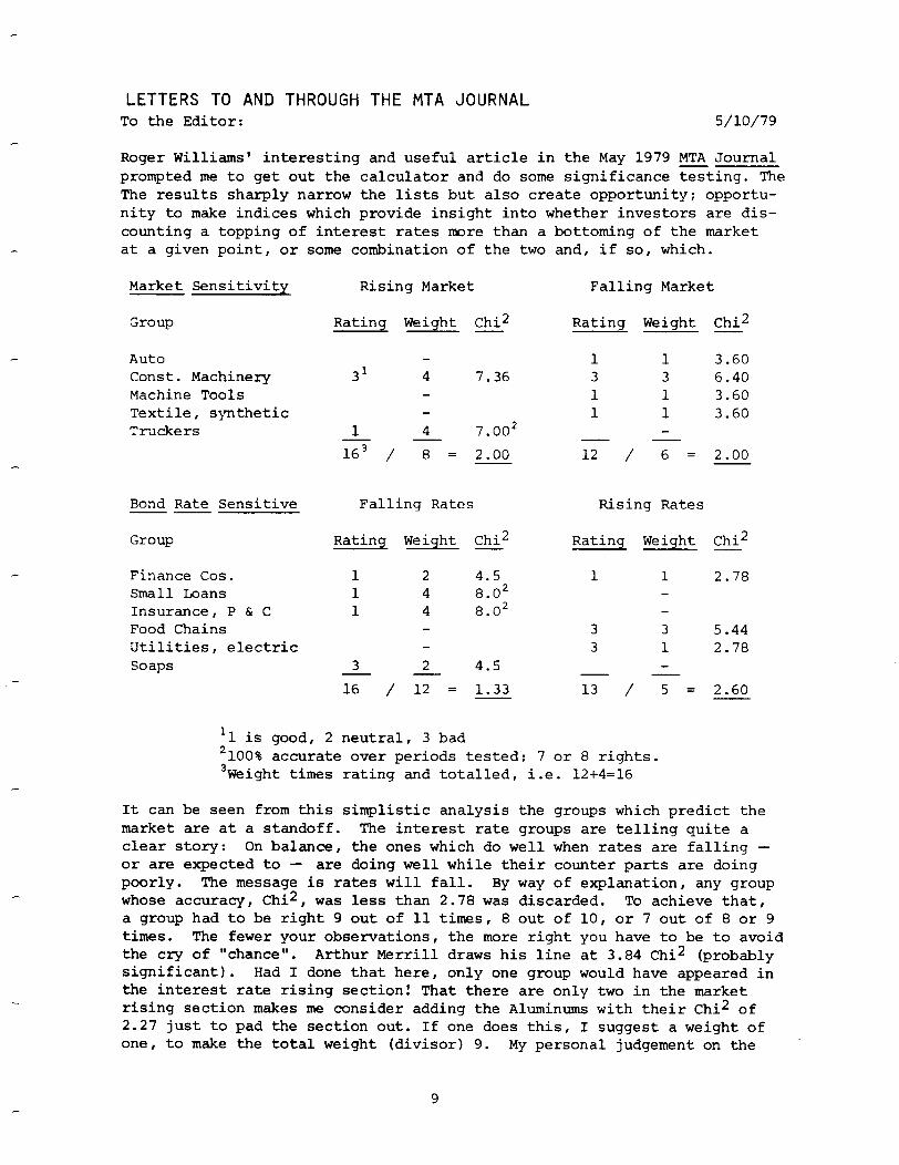
LETTERS TO AND THROUGH THE MTA JOURNAL To the Editor: 5/10/79

Roger Williams' interesting and useful article in the May 1979 MTA Journal prompted me to get out the calculator and do some significance testing. The The results sharply narrow the lists but also create opportunity; opportunity to make indices which provide insight into whether investors are dis- counting a topping of interest rates more than a bottoming of the market at a given point, or some combination of the two and, if so, which.

Market Sensitivity Rising Market Falling Market

Group Rating Weight Chi2 Rating Weight Chi2

Auto Const. Machinery Machine Tools Textile, synthetic Truckers

3l 4 7.36

1 4 7.002

163 / 8 = 2.00

1 1 3.60 3 3 6.40 1 1 3.60 1 1 3.60

12 / 6 = 2.00

Bond Rate Sensitive --

Group

Finance Cos. Small Loans Insurance, P & C Food Chains Utilities, electric Soaps

'1 is good, ?

Falling Rates Rising Rates

Rating Weight Chi2

1 2 4.5 1 4 8.02 1 4 8.02

3 2 4.5

16 / 12 = 1.33

2 neutral, 3 bad

Rating Weight Chi2

1 1 2.78

3 3 5.44 3 1 2.78

13 / 5 = 2.60

'100% accurate over periods tested: 7 or 8 rights. 3Weight times rating and totalled, i.e. 12+4=16

It can be seen from this simplistic analysis the groups which predict the market are at a standoff. The interest rate groups are telling quite a clear story: On balance, the ones which do well when rates are falling - or are expected to - are doing well while their counter parts are doing poorly. The message is rates will fall. By way of explanation, any group whose accuracy, Chi2, was less than 2.78 was discarded. To achieve that, a group had to be right 9 out of 11 times, 8 out of 10, or 7 out of 8 or 9 times. The fewer your observations, the more right you have to be to avoid the cry of "chance". Arthur Merrill draws his line at 3.84 Chi2 (probably significant). Had I done that here, only one group would have appeared in the interest rate rising section! That there are only two in the market rising section makes me consider adding the Aluminums with their Chi2 of 2.27 just to pad the section out. If one does this, I suggest a weight of one, to make the total weight (divisor) 9. My personal judgement on the ~

9

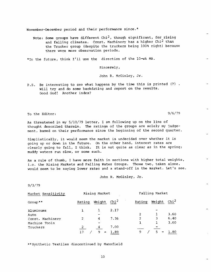
November-December period and their performance since.*

Note: Some groups have different Chi*, though significant, for rising and falling climates. Const. Machinery has a higher Chi* than the Trucker group (despite the truckers being 100% right) because there were more observation periods.

*In the future, think I'll use the direction of the lo-wk MA.

Sincerely,

John R. McGinley, Jr.

P.S. Be interesting to see what happens by the time this is printed (?I . Will try and do some backdating and report on the results. Good God! Another index?

To the Editor: 9/6/79

As threatened in my 5/10/79 letter, I am following up on the line of thought described therein. The ratings of the groups are solely my judgement, based on their performance since the beginning of the second quarter.

Simplistically, it would seem the market is undecided over whether it is going up or down in the future. Cm the other hand, interest rates are clearly going to fall, I think. It is not quite as clear as in the spring; muddy waters run slow, or some such.

As a rule of thumb, I have more faith in sections with higher total weights, i.e. the Rising Markets and Falling Rates Groups. Those two, taken alone, would seem to be saying lower rates and a stand-off in the market. Let's see.


9/3/79

Market Sensitivity Rising Market

Group** Rating Weight G2

Aluminums Auto Const. Machinery Machine Tools Truckers

1 1 2.17

2 4 7.36

2 4 7.00

17 / 9= 1.89

Falling Market

Rating Weight Chi*

2 1 3.60 2 3 6.40 1 1 3.60

9 / 5 = 1.80

**Synthetic Textiles discontinued by Mansfield

10

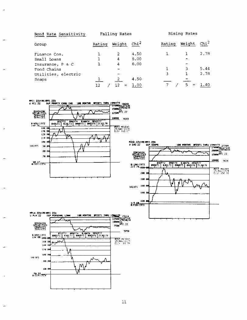
Bond Rate Sensitivity --

Group

Finance Cos. Small Loans Insurance, P & C Food Chains Utilities, electric Soaps

Falling Rates Rising Rates

Rating Weight Chi2 Rating Weight Chi2

1 2 4.50 1 4 8.00 1 4 8.00

1 2 4.50

12 / 12 = 1.00

NPCI zZlKas)(Kc.LN u PC1.22 SLP PWPTV emu INS,

1 1 2.78

1 3 5.44 3 1 2.78

7 / 5= 1.40

N?LN 2mnsMPc zzu

UPLYZZ SL

To the Editor: January 8, 1980

Can't remember if I've sent this to you already, so forgive if duplication.

Being curious, I got out the calculator and did a regression of the numbers As I no

which created the chart on page 60 of the November 1979 MTA Journal. suspected in my previous letter, one must in fact take a loss to face risk by this sample!!

The regression numbers are:

a = -2.51 (Where the line crosses the Y axis, i.e. the point of no risk, sic.)

b = 1.31 (The rate at which the line rises for each unit of the X axis)

r2 = .54 Which means all of this is baloney; the fit is so bad!

I've sketched the line in on the enclosed copy.


.

12

A CONTRARY OPINION

Stan Weinstein The Professional Tape Reader

The way things are going lately, any upmove that lasts longer than 3 weeks and totals more than 40 points is considered a "major rally". The market runs 50 points in one direction, only to reverse and then give it all back over the next few weeks. This is why timing has been so crucial as the market has gone “nowhere fast". It's hard to believe that almost six years ago (March, 19741, the DJI was topping out at 904 after a big intermediate term rally, and just this past October, it again failed at 904.86. More incredible is the fact that solid intermediate term bottoms were hit in 1971 at 791, 1973 at 784, 1975 at 781, 1977 at 793, 1978 at 779 and just two months ago at 792. Obviously, it's not only the economy that is suffering from "stagflation". Even during this very difficult period, there have been good profit opportunities available through the use of market timing and stock selection. Nevertheless, let's face it, it's easier and far more profitable when you get sustainable market moves last- ing years (not weeks) such as we experienced so often during the 1950s and 1960s. I therefore started ruminating a la Humphrey B. Neil1 about whether the market is destined to remain a roller coaster affair during the 1980s or whether there is a good chance that long term uptrends could once again become part of the Wall Street vocabulary.

My conclusion quite simply is positive - I feel that there is an excellent chance that The Dow 1050 will be overcome within the next few years and that growth will replace stagnation in the marketplace. Here's why I feel as I do: first of all, let's look at sentiment and public expectations. After the "Swinging Sixties", expectations were very optimistic about the next decade. Just about everyone and his broker knew that the 1970s were going to be big growth years. They were even affectionately dubbed the "Soaring Seventies" (ten years later, I think most investors would vote for my choice: The Soggy Seventies). As is usually the case, investors and generals fight the last war and mass expectations rarely come true. So it was no surprise that growth disappeared in the 1970s and timing became crucial for survival. Now as we approach the next decade, there is far greater pessimism than at any time since the late 1940s. To see just how fashionable gloom has become, look at the incredible proliferation of

13

of Gloom and Doom Seminars which tell us that Real Estate, Diamonds, Gold, Silver, even Comic Books have been a better inflation hedge over the past 10 years than the stock market. To my way of thinking, Contrary Opinion alone would have to make you feel quite hopeful about the coming decade - but there is more . . .

The Pension Funds (who exert such an important market influence) have become unbelieveably bearish on the market. Look at the accompanying chart. It shows the percentage breakdown (between stocks and bonds) of new purchases by the Pension Funds. A quick glance shows a very interesting fact. In the early 195Os, the Pension Funds put only 20% of their new money into stocks and 80% into bonds. "Groupthink" is dangerous even among sophisticated investors, so it isn't surprising that bonds were near the beginning of a 30 year major bear trend and stocks were just embarking on a close to 20 year super bull cycle. Then in the late 196Os, as stocks were topping out, the Pension Funds started to fight that "last war" and decided stocks were really a better investment than bonds and they therefore put more and more of their money into common stocks. This trend finally reached its climatic peak in the 1971-1972 period when stocks were bought by them right up to the hilt. We were soon thereafter experiencing the 1973-1974 market crash which was the worst smash in over 40 years.

Which brings us up to the present. The great majority of Pension Fund managers have once again learned a lesson and after getting clobbered in common stocks, they are investing less of their new funds than at any time in the past 30 years - even less than in 19501 Unless the laws of human nature have been repealed and psychology and Contrary Opinion no longer mean anything, their current record low level of buying has a very bullish long term meaning. And if it does, and we start to envision how much money could potentially be shifted by this important group into stocks, you can see the incredible potential.

However,there is far more that makes me feel that we could be entering what will come to be known as the "Exciting Eighties". bet's now look at two objective indicators that support this subjective belief of mine. Measuring the number of secondaries can produce a useful longer term indicator. We track this gauge as a 10 week MA to get an overall trend undistorted by a single week's figures. There is no one magic level that flashes a perfect signal,and,over the years, I have had to adjust the parameters downward due to certain secular trends. However,as a rough rule of thumb, up until 1974, the guidelines were that peaks above 60 represented a danger area in the market and bottoms under 15 signalled safe buying areas. Since then, the boundaries have been lowered to 25-30 for a warning signal and 5 or lower for a basing area. Starting with 1960 to give us some historical perspective, readings were extremely low but moved up to a peak of 65 by November, 1961 . . . comfortably ahead of the 1962 crash. The next happening is that

14

DOW JOUES INDUSTRIALS loo0 loo0

900 900

800 800 700 700 600 600 500 500 10 10 WEEK MA. OF SECONDARY OFFERINGS WEEK MA. OF SECONDARY OFFERINGS 150 150 h h

50

’ 1 1965 1 1966 ( 1967 11968 I1369 11970. I1971 1 19721 197311974 ( 1975 (1976 1 1977 I1978 11979 1

the number of secondaries dropped sharply from that high level to a paltry few in June and July of 1962 - right at the bottom for the DJI providing an excellent advance signal for gathering stocks during the Cuban missile crisis that autumn. The number of secondaries remained low all the way through the benign bull years of 1963 and 1964 revealing that it was going to be a long running bullish affair. This indicator did not start upward until the Spring of 1965, when a high near 80 was registered that May. Following a sharp intermediate reaction, the total stayed high during the remainder of that year,just ahead of the 1966 bear market. Then after the market crashed, these insiders did their thing again. A sharp reduction in the number of secondaries followed so that down near the market bottom in September, 1966, the reading got as low as 11. That was a solid signal for a new bull market blossoming. This indicator remained quiet until May 1968 when dumping of big blocks via secondaries started to shoot up again reach- ing a peak in December, 1968 near 95. Once again, that was a great clue signalling the coming 1969-1970 crash. That high level was maintained throughout the first half of 1969 showing it was going to be a long and difficult bear market even after the initial price slide. The next period of extremely low readings came in June, 1970 close to that major bottom as this indicator registered a mere 5 secondaries. After the initial explosive

upleg, a warning was given when the number of secondaries shot up to over 100 in the Spring and Summer of 1971 and remained high despite a steep intermediate term drop in prices that year. Such persistance was an added- and emphatic- warning that the market was in serious trouble. Then in mid- 1972, the 10 week level reached an incredible 161 and you couldn't have ask- ed for a better early warning that disaster lay ahead and the market soon embarked on the worst slide since 1929-1932.

The next important signal was flashed two years later,in the summer of 1974, when there were absolutely no secondaries being offered. Such confidence in holding onto large positions proved to be a terrific early clue for the bottom that came in October, 1974; and as the zero readings continued, a double bottom was made that December. The next trouble spot was June, 1976 as the ratio moved up to 28 (new parameters) which foreshadowed the Septem- ber, 1976-February, 1978 bear slide. In February of 1978 as the market was

15

scraping bottom near 740, the ratio dropped back to a very low 2 which ended up being a signal for the February-September, 1978 upmove. Then,in August of that year,the ratio moved back up to 26 which preceded the 1978 October massacre. Again in February, 1979, the ratio fell to a low of 4 preceding a good move in the market back up toward the 900 area. Which brings us up to the present. Once again, after having moved up to a moderately high level near 20 in October, this gauge has fallen down to a low level of 4. While certainly not a pinpoint guide, based on this indicator alone, it would appear that the odds are overwhelmingly against a major bear market starting in the near future and the probabilities are quite good of a solid bull move.

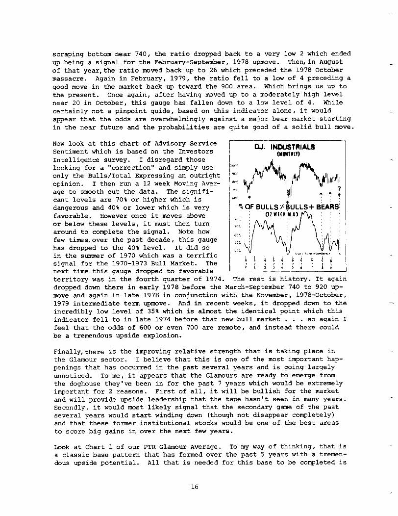
Now look at this chart of Advisory Service Sentiment which is based on the Investors Intelligence survey. I disregard those looking for a "correction" and simply use only the Bulls/Total Expressing an outright opinion. I then run a 12 week Moving Aver age to smooth out the data. The significant levels are 70% or higher which is dangerous and 40% or lower which is very favorable. However once it moves above or below these levels, it must then turn around to complete the signal. Note how few times,over the past decade, this gauge has dropped to the 40% level. It did so in the summer of 1970 which was a terrific signal for the 1970-1973 Bull Market. The next time this gauge dropped to favorable

% CjF BULLS .I $ULLS+ B&S:

territory was in the fourth quarter of 1974. The rest is history. It again dropped down there in early 1978 before the March-September 740 to 920 upmove and again in late 1978 in conjunction with the November, 1978-October, 1979 intermediate term upmove. And in recent weeks, it dropped down to the incredibly low level of 35% which is almost the identical point which this indicator fell to in late 1974 before that new bull market . . . so again I feel that the odds of 600 or even 700 are remote, and instead there could be a tremendous upside explosion.

Finally,there is the improving relative strength that is taking place in the Glamour sector. I believe that this is one of the most important hap- penings that has occurred in the past several years and is going largely unnoticed. To me, it appears that the Glamours are ready to emerge from the doghouse they've been in for the past 7 years which would be extremely important for 2 reasons. First of all, it will be bullish for the market and will provide upside leadership that the tape hasn't seen in many years. Secondly, it would most likely signal that the secondary game of the past several years would start winding down (though not disappear completely) and that these former institutional stocks would be one of the best areas to score big gains in over the next few years.

Look at Chart 1 of our PTR Glamour Average. To my way of thinking, that is a classic base pattern that has formed over the past 5 years with a tremendous upside potential. All that is needed for this base to be completed is

16

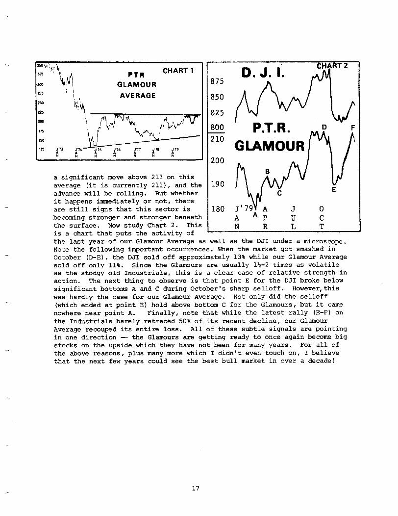
PTR CHART 1

GLAMOUR

AVERAGE

D. 3. I. :zRT2

800 ’ P.T.R. D -“- F

a significant move above 213 on this average (it is currently 2111, and the advance will be rolling. But whether it happens immediately or not, there are still signs that this sector is 180 J 0 becoming stronger and stronger beneath

J’791 t

A K

3 C the surface. Now study Chart 2. Thiz N L T is a chart that puts the activity of the last year of our Glamour Average as well as the DJI under a microscope. Note the following important occurrences. When the market got smashed in October (D-E), the DJI sold off approximately 13% while our Glamour Average sold off only 11%. Since the Glamours are usually 15-2 times as volatile as the stodgy old Industrials, this is a clear case of relative strength in action. The next thing to observe is that point E for the DJI broke below significant bottoms A and C during October's sharp selloff. However,this was hardly the case for our Glamour Average. Not only did the selloff (which ended at point E) hold above bottom C for the Glamours, but it came nowhere near point A. Finally, note that while the latest rally (E-F) on the Industrials barely re.traced 50% of its recent decline, our Glamour Average recouped its entire loss. All of these subtle signals are pointing in one direction - the Glamours are getting ready to once again become big stocks on the upside which they have not been for many years. For all of the above reasons, plus many more which I didn't even touch on, I believe that the next few years could see the best bull market in over a decade!

17

intentionally blank

18

REASSESSMENT OF THE SPECULATIVE AND CONSERVATIVE CYCLES

Charles D. Kirkpatrick II

Like many others, we have long believed that various segments of the stock market act independently of one another. Among these, the most obvious differences have occurred between the speculative and conservative sectors, i.e., between small capitalization and large capitalization issues.' We also have indicated that four-year markets seemed to alternate their leadership between conservative and speculative, a rotation which led us to hypothesize an eight-year period of leadership in which each type of market was repeated eight years later. Therefore, the 1966 market was dominated by speculative issues, the 1970 by conservative, and the 1974 again by speculative. To date, however, the market beginning in 1978 has failed to produce the anticipated reversal back to conservative leadership. Specula- tive indices (American Stock Exchange, for instance,) have made new highs while the conservative (Dow Jones Industrial) has only just recently shown signs of incipient strength. The continued strength of the speculative sector has created the need for us to re-evaluate the validity of our original thesis.

At the suggestion of William Doane, we undertook a study of speculative versus conservative sectors in order to determine if their periodicities were different than the eight years we had originally presumed. In the case of the speculative market, as represented by Standard & Poor's Low Priced Index, we found that the periodicity was still the eight years theorized previously. However, the conservative market had a periodicity closer to 12 years and was considerably less volatile. When we combined the differing periodicities of the two sectors, we found that both sectors occasionally acted in concert with each other, as in 1961 when they both rose. Yet at other times, including the present, the speculative sector

'We prefer to use speculative and conservative as opposed to industry groups, for example, because they are often composed of both sectors and have found that the concept of stock analysis based on a general sense of qual,ity transcends most ordinary methods of categorizing stocks.

19

was in the process of peaking while the conservative sector was still in the process of bottoming out. When the four-year low did occur, conse- quently, it failed to produce the dynamic new leadership which is anticipated when one or the other sector is rising from a low. One year after the four-year low, the conservative sector is beginning to strengthen while the speculative sector is peaking and beginning its relative decline. By re-analyzing the data and determining the different periodicities for each sector, we are able to explain the seeming inconsistency which presently exists between the speculative and conservative issues.

Our data was the annual mean for the Standard & Poor's 500, the Standard & Poor's Low Priced Index, and the Dow Jones Industrial Average. We took the Low Priced Index as representative of the speculative sector, the Dow Jones Industrial as representative of the conservative, and the Standard & Poor's 500 as representative of the entire market. First, we divided each sector by the S&P 500 to eliminate the long bias of a rising market and to dampen the effect of the four-year and other market cycles. Then we again dampen- ed each ratio with a ten year moving average and observed the oscillation of the annual means about that ten-year average in each sector.

Obviously, the speculative sector was more volatile than the conservative and showed an annual mean peak deviation from the ten-year moving average of 30.9%. We also noted that where a trend was drawn through the data, the mean compound annual increase over the S&P 500 was only 0.1% per year. The Low Price Index, therefore, while oscillating rather widely, had only gain- ed slightly over the remainder of stocks in the period from 1928 when it was just introduced. (It might someday be a useful tool in demonstrating that the incurring of risk, as defined by volatility, has not improved performance over long periods of time.)

More importantly, however, we found that the oscillation had a periodicity of roughly eight years, as we had originally suspected. One difficulty in pinpointing the precise periodicity is due to the lack of a sufficient number of cycles since the inception of the index. Whenever the data is limited, the reliability of the results must be suspect. Based on a rather crude inspection of the data, we concluded that a period of 8.17 years exists in the Low Priced ratio. Such a finding is totally inconsistent with our previous findings on similar periods in the ratio of the Low Priced to the Dow Jones Industrial and explains why a speculative period seems to occur in every other four-year market.

Taking the periodicity of 8.17 years and peak deviations from a ten-year moving average of 30.9%, we fitted a cosine formula in order to encompass peaks and valleys as precisely as we could and have plotted the result in the chart at the end of the article. This should represent a rough approx- imation of the behavior of the Low Price ratio (to the S&P 500) about its ten-year moving average.

One factor which we did not assess was the change in makeup of the Index over the period from 1928 or whether or not the stocks included were considered speculative at the various times. We have taken for granted that such considerations are not of extreme importance in this study.

20

One of the most interesting results of this study was that the conservative sector was not dominated by the eight-year periodicity. Again we took the average (Dow Jones Industrial), divided its annual mean by that of the S&P 500 to be declining at a compounded rate of close to 5%, although for our purposes, this was immaterial because the moving average screened out the trend automatically.

Naturally, the oscillations of the conservative ratio about its moving average were considerably less than those of the more speculative sector averaged only 6.0% of the moving average value. Compared to the speculative sector, which oscillated 30.9% about its moving average, the conservative sector looked quite calm. One of the reasons for the earlier assumption that an eight-year alternating period existed in the two sectors was that the speculative sector, with its eight-year periodicity, oscillated so strongly that it tended to hide the less volatile action of the conservative sector. An eight-year periodicity had been assumed for the conservative sector only because when compared to the large motion of the speculative, it seemed to oscillate in the opposite direction. We found, however, that this sector instead had a periodicity of closer to 12 years, but because of its lesser strength, this periodicity had been overlooked before.

When we examined the Dow Jones Industrial Average prior to 1928, we found that the periodicity had changed during the 1930s from that of an eight- year periodicity. We presume that before the 1920s and 193Os, the Indus- trials were considered more speculative and, therefore, followed the speculative periodicity of nearly eight years. For example, previous to the 192Os, railroads were considered to be conservative and, for that period, rail averages show a cyclicality of closer to 12 years as the conservative industrials show today. Because of the change in periodicity in the 192Os, however, fewer examples than we would prefer exist, and we must, therefore, again warn that this estimate for periodicity may have a large error factor. Keeping in mind these limitations, our best estimate is 11.9 years which closely approximates three four-year markets. This observation partially helps to explain why the current market which we thought would be dominated by conservative issues has failed to do so.

We also fitted a cosine formula to the peaks and valleys of the conservative sector and plotted the results of the ideal periodicity and effect on the chart at the end of the article. The lesser oscillation strength is readily apparent when compared to the oscillations of the speculative sector. In the lower portion of the chart, we plotted the differences between the two idealized cycles to give an idealized view of how the speculative sector would appear to the conservative. We also superimposed the actual values for the speculative sector less the conservative in order to demonstrate how well the combination of the two ideal segments parallel the actual numbers and how well they explain the present.

In the early 196Os, the speculative top in 1961 was accompanied by large moves in both the speculative and conservative sectors. While the domi- nance of the speculative sector, because of its larger volatility, over- shadowed the conservative move, its actions become quite clear on the

21

chart where idealized waves are portrayed. The speculative peak in 1968 was accompanied by very little action in the conservative sector and this is again demonstrated in the idealized versions of each sector. The current market shows that a peak in the relative strength of the speculative issues has been seen. Because of its extra length, however, the conservative cycle is not due to strengthen significantly until next year. Where before we had assumed a simple rotating leadership between speculative and conservative, because of its longer periodicity conservative leadership can occur later, as it will next year.

Our analysis of the parts, therefore, has explained why the whole has not performed as expected previously. The conservative sector is not quite ready, the speculative is dying , and a conspicuous lack of leadership pre- vails. Those fears which are based on the expectation of a large market drop due to the failure of the Dow Jones to lead should be allayed.

rlllllllrl~llllll rlllllllllllllil ’ ' ' 50 55 60 65 70 75 80 $5

I iDEAL SLP LOU PRICE S6P 500

SLP LW PRICE Dou JONES INDUSTRIAL -- S6P 500

r\ I I

IDEAL MTA JONES INCUSTRIAL Sa? d-

30 H 60 65 m 75 80 95

, I, 1 I I I I I I I1 III, I1 .il I I I Ill I bl I I III CJ

DEPARTURES FROM TEN-YEAR MOVING AVERAGE

22

CYCLICAL PHENOMENA

Bernard Fremerman

Over the years, man has shown an inclination to disbelieve new scientific evidence which later proves to have tremendous influence on the sum of human knowledge. In the early 17th Century when Johannes Kepler first proposed that the moon, through some mysterious force, was the cause of the tides here on Earth, the scientific community dismissed his idea as nonsense. It wasn't until some 40 years later when Issac Newton proposed his laws of motion and gravitation that Kepler's idea was accepted. Like- wise, Kepler's concept of the three basic laws of the motions of planets was ridiculed by contemporary scientists, only to be validated later by Newton's work. If the work of Kepler and Newton had never been done, and if today's scientific community were presented with the concept that the moon and sun cause the ocean's tides,it is highly unlikely that this idea would be accepted. It would,in fact,be considered most "meta-physical".

In the early part of the 20th Century, Albert Einstein proposed his Special and General Theories of Relativity. For at least 10 years the scientific community would not accept them because,axmong other things, it meant that their basic concept of the universe had to be restructured. Even as late as 1941,German scientists derided Einstein's theory as "The Jew Theory" of relativity.

I believe that civilization is on the verge of another major breakthrough in human knowledge, whose effect could be as profound as any heretofore seen. It may well give us a better understanding of human behavior, natural phenomena and man's relation to his environment. Bits and pieces of evidence exist in such diverse fields as natural science, wars, economics, health, biology and radio interference which suggest that regular periodicity exist in events, and that such periodicities seem to have some correlation to extra-terrestial phenomena. The entire subject is a massive jig-saw puzzle, but we have enough expertise in science today to unravel some of these mysteries.

The man who has probably contributed the most to this entire area of study is the late Edward R. Dewey, former director of the Foundation for the

23

Study of Cycles, in Pittsburgh, Pennsylvania. Some of the more notable people who have served on the Board of Directors of the Foundation include Charles G. Abbot, retired secretary of the Smithsonian Institution; Harold E. Anthony, curator of the Frick Laboratory at the American Museum of Natu- ral History; Vice Admiral (retired) Harold G. Bowen, United States Navy; John Q. Stewart, Professor of Astronomical Physics at Princeton; Lord Beveridge, the English economist: Donald Herzberg, Dean and Professor at Rutgers University; Max A. Lauffer, Jr., Andrew Mellon Professor of Bio- physics at the University of Pittsburgh, and Harlow Shapley, former director of the Harvard Observatory.

Dewey had spent over 40 years collecting evidence and trying to fit the pieces together,although he was not the first. Many others have contributed extensively to the subject in various diciplines. It is my purpose to outline some of the more significant work that has been done and which has come to my attention. All of the research outlined here can be documented.

Economics

One of the first proposals that sunspots might have a relationship to human affairs was suggested in 1801 by Sir William Herschel, an astronomer who called attention to a correlation between sunspot activity and the price of wheat. Thirty or forty years later, Dr. Hyde Clarke of England took note of an 11 year cycle in trade and speculation and advanced the idea that there might be a physical cause. In 1860, a Frenchman, Clemet Juglar discovered an economic cycle of about 8 to 10 years. In 1878, W. Stanley Jevons, a British economist,noted a relationship between economic enthusiasm and increased sunspot activity. Economists generally tend to dismiss this theory as an intellectual pursuit without foundation.

In 1881, an English astronomer, N. R. Pogson found a connection between sunspot activity and the price of grain in India. In 1919 Professor Ellsworth Huntington of Yale suggested that solar radiation had an effect on human beings, and this in turn on business conditions.

In 1913, a Dutchman, J. van Gelderen also noted a 10 year cycle in economics, as well as a much larger one extending over several decades. In 1926, a Russian economist, Nicolai Kondratieff,wrote of a long term cycle of 50 to 60 years in economics. About the same time Joseph Kitchin noted an economic cycle of about 40 months. In 1934 an economic study of "Solar and Economic Relationships" was prepared by Dr. Carlos Garcia-Mata and Felix I. Shaffner of Harvard University. This study was published in The Quarterly Journal of Economics. They set out to disprove Jevon's ideas and ended up confirming and elaborating on them.

Edgar Lawrence Smith, a member of the Royal Economic Society wrote a series of books isolating and exposing economic cycles of various periodicities. In 1959 he published Common Stocks and Business Cycles which re- lated economic phenomena to planetary orbits. In 1965, Charles G. Collins an investment adviser, wrote in the Financial Analysts Journal that the largest percentage stock market declines since 1971 have coincided with

24

sunspot data, and the influence of Mercury depends on the phases of Venus, Earth and Jupiter. Writing in Nature, November 10, 1972, K. D. Wood found a close relationship between the computed tidal force of these same four planets and the 11.1 year sunspot cycle.

Radio Wave Interference --

Before his retirement from RCA Communications Company in 1968, John H. Nelson was assigned the task of predicting short-wave radio interference. He discovered that specific patterns of heliocentric positions of the planets seemed to have a strong correlation to such interference. His accuracy in predicting the daily timing and amount of radio disturbances was better than 90 percent over an extended number of years. He has been a consultant to NASA and to Jet Propulsion Laboratories, using his techniques to predict solar flares and radio interference. I spoke with Mr. Nelson recently and he told me that he has also noticed that planetary alignments seem to correlate to terrestial earthquake activity. This dis- covery seems to confirm the work of John R. Gribbin and Stephen H. Plagemann, two astrophysicists, in their book The Jupiter Effect. The basic thesis of their work is that because of gravitational forces, geocentric planetary alignments trigger off earthquakes and that a major grand alignment is due in 1982 - an event that occurs every 179 years.

Sociological

In 1926 Professor A. L. Tchijevsky of the University of Moscow presented a paper to the American Meteorological Society in Philadelphia outlining an index of mass human excitability which manifested itself in waves of about 11.1 years and correlated with the 11 year sunspot cycle. He wrote: "The maximum of human activities in correlation with the maximum of sunspot activity, expresses itself in the following:

a. The dissemination of different doctrines (political, religious, etc.) the spreading of heresies, religious riots, pilgrimages, etc.

b. The appearance of social , military and religious leaders, reformers, etc.

C. The formation of political , military and religious and commercial corporations, associations, unions, leagues, sects, companies, etc."

Biological and Medical

Medical and biological effects of solar forces have been documented for years by doctors and scientists. In 1920 a French physician, Dr. Maurice Faure and an astronomer, M. Vollet collaborated on a study which showed a relationship between greater sunspot activity and a higher rate of sudden deaths.

A. L. Tchijevsky, referred to earlier in this paper, also noted that diph- theria, cholera, typhus, small pox and influenza reached peak proportions

25

or followed the year in which average sunspot numbers have reached fifty.

I became interested in cyclical research after having accidentally stumbled on it in October of 1975. With the help of several friends and a computer we were able to define and isolate one very regular cycle that has persisted in the price of two different stocks listed on the New York Stock Exchange. Trading on the basis of this one cycle alone between 1970 and 1976, would have yielded a profit to loss ratio of about 3 to 1 in one stock and 2 to 1 in the other. This cycle also appears in the Dow Jones Industrial Average, although it does not seem as pronounced in previous years going back to 1963. It may be coincidence, but we find a strong correlation between this cycle and a unique astronomical observation.

There are faint hints that some of the longer term economic cycles are trending downward at the present time, and may "bottom out" over the next 5 to 25 years. If those cycles represent reality, they might well foretell major world-wide economic and social upheavals. It would seem a good idea to find out about them as soon as possible.

It is noteworthy that a number of economists have made contributions to this area of knowledge, but because of "conventional wisdom" their contemporaries have refused to accept them. It is, after all, a bit dis- turbing to man's ego that his economic decisions might be controlled by some "mysterious" forces.

Wars

In 1936, Loring B. Andrews, a Harvard astronomer found a correlation over a 200 year period between sunspot activity and wars and international crises. The late Professor Raymond H. Wheeler while at the University of Kansas compiled an Index of International War Battles and Civil War Battles, as- signing numerical ratings to every recorded engagement extending back to 600 B.C. In 1950 the Foundation for the Study of Cycles researched Profes- sor Wheeler's work and was able to isolate four repeating cyclical patterns in the Index of International Battles. These cycles were of 142 year, 57 years, 22.14 years and 11.2 years. The combination (synthesis) of these four cycles has held a close relationship to the ebb and flow of intema- tional battles up to the present time. This synthesis also forecasts a major peak in international battles for about 1982. Later, the Foundation isolated five additional periodicities in the war index. Including these cycles indicates that ideally, the war cycles peaked in the mid-1970s and are now in a down-trend.

Astronomical Studies

A number of contemporary astronomers have published scientific papers describing a relationship between planetary positions and solar activity. To my knowledge, none of them have attempted to relate these alignments to terrestial events. In 1965, Paul D. Jose writing in the Astronomical Jour- nal,disclosed a 178.7 year periodicity in the positions of planets, the sun's motion and in sunspot numbers. In a 1972 issue of the same publica- tion, E. K. Bigg has shown that the period of Mercury's orbit appears

26

-

at times of maximum solar disturbances. An interesting and timely observation concerning influenza is that the three major epidemics in this century, the Swine flue in 1918-19, the Asian flu in 1957-58 and the Hong Kong flu in 1968-69 all coincided with the peak sunspot activity in the 11.1 year solar cycle.

In the early 1930s Maki Takata, a Japanese doctor developed a method of determining when a woman was fertile by studying her ovarian cycle. He utilized a chemical reaction test of the albumen in blood serum. He found that the activity of the albumen fluctuated to enable him to know at what stage his patients were in the ovarian cycle. Similar tests of the blood serum of male patients did not show this fluctuation. In 1938 doctors all over the world were using "The Takata Effect" when they suddenly reported that the test results were varying widely and randomly in both male and female blood samples. Subsequent investigation revealed that these random movements occured simultaneously all over the world. Dr. Takata performed a series of tests over the next 20 years and found a definite relationship between changes in the chemistry of blood serum and changes in solar activity.

In 1934 two German researchers, Bernhard and Traute Dull found a relationship between tuberculosis deaths and violent solar explosions. In 1942 two German doctors Back and Schluck discovered that eclampsia, a convul- sive attack during preganacy, is more prevalent on days when the sun had been active. In 1952 Dr. Lingemann of West Germany found a relationship between the incidence of pulmonary hemorrhage and solar activity.

The work of Soviet Hemotologist Nicolas Schulz, published in 1960 showed a relationship between the increase in lymphocytes in human blood and solar activity. Between 1954 and 1960 Professor B. De Budder of the Uni- versity of Frankfurt-am-Main, Professor Romensky, Soviet physician, Dr. Giordano of Pavia, Italy and French physician Poumailloux all have shown evidence of the interrelationship between solar activity and various physical disorders of the human body.

The work of Professor Frank Brown of Northwestern University has revealed a number of incredible extra-terrestial (solar and lunar) phenomena that are correlated to biological changes in plant and animal life. He found that he can influence the direction of movement of flatworms by placing them in magnetic field.

Oysters open and close their valves in harmony with the tides. Dr. Brown removed a group of oysters from the waters of New England and transported them to Evanston, Illinois. Within a few weeks, these oysters had changed the rhythm of opening and closing their valves so that they were in syn- chrony with what the tides would have been at Evanston if there was an ocean there.

Dr. Brown has also conducted experiments with potato plants. He has measured the amount of oxygen given off by these plants and finds a strong cycle of 23 hours, 56 minutes and 4 seconds in their oxygen emission. There seems to be no explainable mechanism, but the period of this cycle

27

corresponds precisely to the length of the disereal day - which is the time it takes for the earth to make one revolution with respect to the stars beyond our solar system.

In Syracuse, New York, Dr. Robert 0. Becker, an orthopedic surgeon has observed that when he exposed rats to a 60 hertz field they exhibited hor- monal and biochemical changes similar to those caused by stress. Dr. James H. McElhaney of West Virginia University found that low frequency electric fields can cause bone tumors in rats.

A physician at the University of Southern Illinois, Dr. Ame Sollberger, has done extensive research into biological rhythms in the human body, and a book published in 1971, Body Time,by Gay Gaer Lute, details literally hundreds of experiments by medical doctors and biologists in human and biological body rhythms, many of which are in harmony with extra-terrestial phenomena.

One other piece of research that was done by a contemporary French psychol- ogist Michel Gauquelin deserves mention as incredible as it sounds. In a book published in 1973, Cosmic Influences on Human Behavior, he details a -- study of 25,000 celebrities in Germany, Italy, Belgium and Holland. He found that the positions of the planets at the precise time of birth had predictive capabilities insofar as the profession of these 25,000 people was concerned. His work was checked and verified by a number of scientists including Dr. J. Allen Hynek, Chairman of the Department of Astronomy at Northwestern University, who wrote the introduction to his book.

The Mechanism

In my limited view, it seems that the mechanism which functions in all of these phenomena is either electro-magnetic or gravitational. (According to Martin Gardner, a writer for Scientific American, Einstein and others have suspected that these two forces have something in common and have tried to develop a "Unified Field Theory" that will unite gravity and electromagetism in one set of mathematical equations, but no one has yet been successful.) I see all biological organisms as sensitive electronic "receivers" responding to very subtle signals from the cosmos. I believe that the sun is an important link to this whole phenomenon. I am hopeful that further research can be undertaken to either prove or disprove this thesis.

As I see it, there are two basic approaches to be taken, although other avenues may exist and prove even more fruitful. The first approach involves wave form analysis - that is analyzing empirical data for evidence of recurring periodicities. This is basically the approach of Dewey. The second approach involves heliocentric and geocentric planetary positions and relating them to terrestial events, the form of research taken by Nelson and being undertaken by the Foundation for the Study of Cycles.

I feel that even though these cyclic phenomena are influences, they are not the whole story. There are likely many random forces in effect too. All of the evidence is not in, but that which exists is too strong to deny.

28

The Paradoxical Nature of Cycles -

A most difficult aspect of cycle study to comprehend parallels Heisenberg's Uncertainty Principle. In sub-atomic physics, the exact position of an electron can be determined. However, the simultaneous determination of its speed and direction is not possible. Conversely, the speed and direction of an electron can be determined,but its position cannot be simultaneously located. As a matter of fact, physicists believe that the very act of observing the phenomenon changes the behavior patterns - a most difficult set of circumstances with which to deal.

In studying cycles of human behavior,we encounter similar difficulties. We humans who are observing our own behavior are also part of the phenomenon. How does our observation (and action) affect the results? For example, suppose that a set of real cycles exist in the price of the common stock of XYZ Company. And suppose that "everyone" is aware of them. How will this knowledge affect the outcome? Will such knowledge become a self- fulfilling prophecy or will it negate any predicted future action in the price of the stock? The entire subject has an "Alice-in-Wonderland" character to it which strains our perception of reality.

A Course of Action - -

Some of the people engaged in cycle research see potential economic and social upheavals in the near future. Some feel that the forces in motion are already irreversible. There are two major areas of concern.

The first involves the economy. Preliminary long-term cyclical analysis indicates that there is a good probability that we have at the most, five or six years before severe world-wide economic resession sets in. The second area of potential catastrophy is the possibility of major intema- tional war, also indicated by long term cycle studies.

Man, through his greed and short-sightedness, has shown an inclination to step rough-shod over his fellow man in the name of economic advance. The possible collapse of the world's economy and the potential destructiveness of another major war will be the direct result of man's lack of wisdom in guiding his won destiny and his lack of awareness of a major force behind his irrational behavior.

We need not look very far to see the evidence. We recently emerged from a war which was one of the most costly adventures in which our country was ever involved - both in terms of blood and in terms of economic resources. This was indeed one of the greatest monuments to our own igno- rance and irrationality.

A second monument exists in the field of economic planning. If we question the top ten expert economists in the world, as to the causes of our economic problems and ask them for suggestions for a remedy, we will likely get ten different opinions - each delivered with forcefulness and with resounding authority. I believe that the truth of the matter is that none of them really know because none have the whole picture.

29

It is imperative that immediate consideration be given to undertake careful scientific studies to either confirm or deny the reality of regular periodic cycles in war and economics. A great deal of work has already been done, and it is my belief that we are on the verge of becoming aware of the causation.

If we unscramble some of these mysteries we might be able to ward off or at least limit the destructive effects. It is hoped that this paper will stimulate sufficient interest to encourage someone to provide the needed financial means to carry out the needed research.

December 1, 1976

(Revised December 18, 1978)

30

ELLIOTT IMPULSE

Henry 0. Pruden, Ph.D.*

Some powerful, mysterious and beneficent force must be evolving. A first impulse from it has blessed us with two fine books on the Elliott Wave Prin- ciple: Robert C. Beckman, Supertiming: The Unique Elliott Wave System (published in 1979 by the Library of Investment Study, P.O. Box 25177, Los

-Angeles, CA. 900251, and A. J. Frost and Robert E. Prechter, Jr., Elliott Wave Principle: Key to Stock Market Profits (published in 1978 by New Classics Library, P.O. Box 262, Chappaqua, New York, 10514).

Not only have these two books mysteriously appeared at approximately the same time, but they are mysteriously parallel to each other in purpose, resources, content and format. Both books are written for the serious (sophisticated?) student who has not yet incorporated Elliott analysis into his (her) technical repertoire. Beckman, Frost and Prechter propose to enable us to conduct our own Elliott Wave Analyses. They justly assume that there is a scarcity of handy references on Elliott's approach; they do us a service by admirably filling this void.

A similarity between the two books no doubt stems from a commonality of resources: R. N. Elliott's original The Wave Principle (Financial World, 19381, Elliott's magnum opus, Nature's Law (1947) and the various works of Hamilton Bolton (circa 1960). The precepts found in these resources are faithfully recorded in the books' contents, where the reader immediately encounters Elliott's basic assumption that the market evolves in a law- like pattern of five upward zig-zagging waves and three downward corrective waves. Both books then lead you on an excursion through the arcane world of Fibonacci and mathematical foundations, show you the hierarchy of wave order, spell out correct wave counting procedure, and explain the use of channeling, ratios, time periods, complementary approaches and indicators.

*Dr. Pruden is a private investor, a Lecturer at Golden Gate University and a member of the Board of Directors of the Technical Securities Analysts Association of San Francisco, as well as a subscriber to the MTA.

31

These alone are worth the cost. Yet these books'greatest wealth lies beyond this in the guidance these authors provide the student for getting through such Elliott labyrinths as alternations, corrections, extensions, irregularities and the many other exceptions to the rule which deter or detour so many students. Both books are good at careful explanations and are amply illustrated with charts.

The differences between the books lies in style and emphasis, which mirror the personalities and surroundings of the authors. Beckman is an American in London who exposes the reader to share-price behavior there as well as in the U.S.A. His deft handling of Elliott applications conveys a deep personal appreciation of Elliott analysis, born from closely following the market via the Wave Principle. Frost and Prechter, who also enliven Elliott examples with their own experiences, are almost in a direct line of descent from Elliott and Bolton, with Frost forging a link from them to the newer generation represented by Prechter. In keeping with the rich tra- dition of this lineage, Frost and Prechter ably carry out a supercycle pro- jection of the Dow Jones Industrial Average.

Beckman, Frost and Prechter are avid prosylitisers of the Elliott Wave Principle, which they sincerely believe possess key, unique powers of market timing. Give them a try . . . they might convert you.

32

The Timely Demise of the Random Walk

Richard C. Orr*

1. Introduction The foundations of technical analysis lie in several key assumptions.

Among these are the existence of areas of support and resistance, which are horizontal boundaries to stock price movement, and the existence of trend lines together with their

more general forms such as moving averages or cycles. The original random walk theory as applied to the movement of stock prices directly challanged these assumptions and hence

the whole area of technical analysis. The random walk model asserts that at any given time the probability is p that a stock price will rise and the probability is l-p that it will fall, where p is some fixed constant. If p is either less than l/3 or greater than 2/3, so that the probability of a move in one direction is at least twice that of the probability of a

move in the other direction, then, if the random walk model is valid, we can easily determine stock trends. However, if p is l/2, or some value close to l/2, then the validity of the random walk model for stock price movement would imply that most of technical analysis and fundamental analysis are useless as methods for forecasting stock prices.

The statistical experiment described in this paper, therefore, has been designed to refute the applicability of this model as a realistic description of stock price movements.

Subsequent modifications of the random walk model, such as Cootner’s random walk within reflecting barriers, are much more compatable with technical analysis and will not be discussed here. * *

*Dr. Orr is Associate Professor and former chairman of the Department of Mathematics,

State University of New York, Oswego, New York. He is currently a consultant to Pershing & Company, New York.

**For an excellent exposition of much of the early work supporting and rejecting the random walk model see Cootner, Paul, The Random Character of Stock Market Prices,

---- M. I.T. Press, 1964.

33

2. A Brief Review of Hypothesis Testing. Before describing our experiment in detail, we turn first to a simpler

example as a means of reviewing the relevant statistics.* Suppose in observing a particular

roulette wheel over a reasonably long period of time we feel that black numbers are winners much more frequently than are red numbers. How do we test to see if the wheel

is biased in favor of black numbers? First, we formulate the null hypothesis, namely: that

the wheel is fair; black should occur as often as does red “in the long run”. Next, we formulate the alternative hypothesis, namely: the wheel is unfair. The occurrences of red

and black numbers in random spins of a roulette wheel which is fair are described by a

particular probability distribution and there is a small chance, even with a fair wheel, that we might still have, say, twenty black numbers occur in a row. Therefore, we must also set the tolerance for error which we will accept, known as the level of significance of the experiment. Suppose that we decide to test the hypothesis that black and red numbers have an equal probability of occurring at the -01 level of significance by recording a total

of 100 red or black numbers, while ignoring any green numbers.** If we are able to reject the null hypothesis, that the wheel is fair, at the .Ol level of significance then we will have

a result which 99 out of 100 times is due to the fact that the wheel is unfair, but 1 out of 100 times is due to an unusual occurrence in the experiment. This kind of result is similar to the conviction of a defendant in a court of law because the jury was convinced of his guilt “beyond a reasonable doubt”. Our “reasonable doubt” in this example is the .Ol probability of error. If, on the other hand, we fail to reject the null hypothesis at the .Ol level of significance, this does not mean that the null hypothesis is correct with

probability .99. To continue our analogy to a courtroom situation, the defendant is presumed innocent until proven guilty beyond a reasonable doubt. Failure to convict could mean that the defendant was innocent, but it could also mean that while he was guilty, there was simply not enough evidence to be found to allow a conviction, given

that the jury must be 99 percent sure before finding the defendant guilty. Note that juries don’t find defendants “innocent”, they find them “not guilty”. Returning to our

experiment, suppose that our sample yields 70 black winners and 30 red winners. The wheel could be unfair if it tends to give us either too many black numbers or not enough

black numbers as winners. Thus our .Ol chance for error must be divided into a .005 chance for too many black numbers and a .005 chance for too few of them. A test of this type with two alternatives is called two-sided. Checking statistical tables we find that for

a fair wheel the probability of 70 black winners in 100 spins is less than .005 and hence

we reject the null hypothesis in favor of the alternative hypothesis that the wheel is unfair.***

*This material can be found in any introductory text for mathematical statistics, for example, Johnson, R., Elementary Statistics, Second Edition, Duxbury Press, 1976.

**Recall that the house’s edge in roulette is created by placing a 37th number, 0, on the wheel in Europe and, additionally, a 38th number, 00, on the wheel in the United States. In our experiment, any spin resulting in 0 or 00 as a winner will simply be disregarded.

***This binomial distribution can be approximated by a normal distribution with mean 50 and standard deviation 5, so 70 is about 4 standard deviations above the mean, after

a continuity correction.

34

On the other hand, an outcome of 60 black winning numbers would not give us sufficient evidence to reject the null hypothesis at the .Ol level of significance. Again, such a result would not imply that the wheel was fair, but merely that we were unable to be 99

percent sure that it was unfair.

The important idea to keep in mind, then, is that in testing stock price

movements against a random walk model, failure to find a significant difference in the two does not imply that they are the same.

3. Description of the Main Experiment. It seems clear that the variation of stock prices, defined mathematically to

be the sum of the absolute value of the changes in these prices, is so large compared to the net change, even over a fairly short period of time, that any statistical test based

entirely on the correlation between successive changes would not yield meaningful results. If the hypothesis that stock prices change in a random manner is to be decisively

tested, we need to find a way to prevent the stock’s deviation in price movement from a random walk model while the stock is in an uptrend from nullifying the deviation which

occurs when the stock is in a downtrend. The following experiment solves this problem by focusing on time rather than on price change.

We will base the null hypothesis on the assumption that at any time a

given index or stock price has an equal probability of rising or falling. A more general case will be mentioned later. We will attempt to reject the null hypothesis at the .OOOOOl level

of significance, In other words, we will only allow a chance for error in this experiment of one in one million.* We will ignor any changes which are equal to zero, so in our

sequence of prices each term is either higher or lower than its predecessor. A peak in prices is defined to be any price which is higher than both its predecessor and its

successor, while a trough is defined to be a price which is lower than both its predecessor

and its successor. We measure the average number of time intervals (days, weeks, months, etc.) either between successive peaks or between successive troughs. A graph of the random walk model appears on the next page. Assuming the null hypothesis to be correct, the distribution of the number of days between peaks or troughs should have

mean equal to 4 and standard deviation equal to 2. A derivation of these results appears in an appendix to this paper. The length of time between successive peaks or troughs is certainly less strongly correlated to the trend of the prices than would be changes in the prices themselves. Hence, at the outset, we would appear to have a better chance of

resolving this issue than have others in the past. The null hypothesis is that in the population from which we sample, the mean number of days between successive peaks (or troughs) is 4. The standard deviation for this population is 2.

*This is ample for our purposes. The actual prob-value, the best possible level of

significance at which we could still reject the null hypothesis, is closer to 10m20.

35

Graph of the Random Walk Model with p =.5

M is a peak which is actually formed the succeeding day (week, month, etc.) when the stock price reaches S. The next peak will be formed on the first day that the price falls after having risen. For example, the peak at N is formed one day later when the stock price reaches F. In this example, the “distance” between M and N is three days. Because the number of days between peaks is equal to the number of days between the points at which the peaks were actually formed, we could measure the distance from S to F rather than from M to N, if it was more convenient. By symmetry, if the above graph is reflected so that all moves up become moves down, and conversely, then we have a model describing the distances between successive troughs.

36

Our sample consists of 1369 consecutive values, from July 5, 1973 to

December 29, 1978, of the Indicator Digest unweighted index of 1500 NYSE stocks,

better known as IDA. This is an appropriate set of data, since under the null hypothesis, if stock prices move at random then so must the IDA. Another experiment using only

data on individual stock prices appears in the next section. The IDA data contains 246 troughs and 245 peaks (these numbers can never differ from each other by more than one). Because a trough appears before a peak in the data, we measure the distance

between consecutive troughs, but equally impressive results would be obtained by measuring the distance between consecutive peaks, instead. The first trough in our data

occurs on July 9, 1973 while the last trough occurs on December 28, 1978. This yields 245 distances with a sample mean equal to 5.57. The Central Limit Theorem tells us that a sampling distribution of sample means is normally distributed (within our tolerances)

with mean equal to 4 and standard error equal to 2/m This implies that our sample mean of 5.57 is more than 12 standard deviations above the population mean!* As this is a two-sided test we need to ascertain whether or not a z score this large can occur with

probability greater than .0000005. A quick check of a normal distribution table tells us that indeed it cannot occur with that large a probability. We therefore reject the null hypothesis that these prices behave like a random walk with p = l/2.

Using a derivation similar to the one given in our appendix, we can show that the generalized random walk model, with the probability of a stock rising equal to p,

has its mean number of days between successive peaks (or troughs) equal to l/p(l-p). Note that if the probability of a stock falling is p, then its probability of rising is l-p and

we again have the mean number of days between peaks (or troughs) equal to 1/(1-p) (1-(1-p)) = l/(1-p)p. While the IDA data previously discussed would not reject the

null hypothesis that the mean is l/p(l-p) for, say, p=3/4, some of the data in the next

section will place even this hypothesis in jeopardy. Not withstanding that, I suspect that most of us would be delighted to have a 3 to 1 edge in forecasting current price changes.

*Recall that the equation for z score is

where 2 =5.57, & =4, < =2, and X =245.

Hence, z =12.287.

37

4. Individual Stocks: Preliminary Results. In the following experiments, approximately 120 consecutive prices (daily

or weekly) for individual stocks are investigated. This sample size is barely large enough to give any results which might be considered meaningful. Time constraints forced the use

of data which, for the most part, was readily accessable by our computer. Any reader

with an interest in this kind of investigation who has rapid access to perhaps one or two thousand consecutive prices for a fairly large number of stocks is urged to repeat these experiments with his or her own data.

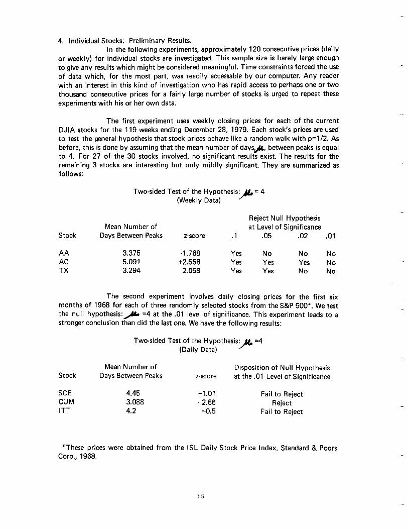
The first experiment uses weekly closing prices for each of the current

DJIA stocks for the 119 weeks ending December 28, 1979. Each stock’s prices are used to test the general hypothesis that stock prices behave like a random walk with p=1/2. As

before, this is done by assuming that the mean number of days& between peaks is equal to 4. For 27 of the 30 stocks involved, no significant results exist. The results for the

remaining 3 stocks are interesting but only mildly significant. They are summarized as follows:

Two-sided Test of the Hypothesis: F

=4

(Weekly Data)

Stock

AA

AC TX

Mean Number of

Days Between Peaks

3.375

5.091 3.294

z-score

-1.768

+2.558 -2.058

Reject Null Hypothesis

at Level of Significance

.l .05 .02 .Ol

Yes No No No Yes Yes Yes No Yes Yes No No

The second experiment involves daily closing prices for the first six months of 1968 for each of three randomly selected stocks from the S&P 500”. We test the null hypothesis:,& =4 at the .Ol level of significance. This experiment leads to a

stronger conclusion than did the last one. We have the following results:

Two-sided Test of the Hypothesis: P

=4 (Daily Data)

Stock

SCE CUM ITT

Mean Number of Days Between Peaks

4.45 3.088

4.2

z-score

+1 .Ol

- 2.66 +o. 5

Disposition of Null Hypothesis

at the .Ol Level of Significance

Fail to Reject Reject

Fail to Reject

*These prices were obtained from the

Corp., 1968.

ISL Daily Stock Price I ndex, Standard & Poors

38

One interesting point to note is that since, for any p between 0 and 1, l/p(l-p) is never less than 4, (in hindsight) we could have rejected a null hypothesis that stocks behave like a random walk for any fixed p, using the sample of prices for Cummins Engine Co. stock.

5. Summary The daily price study of CUM allows us to reject the hypothesis that stock

prices behave like a random walk. The level of significance (.Ol) is good,* but experiments involving a much larger set of data would probably yield more powerful results. For completeness, the DJIA weekly price experiment is included, although the results are not really satisfactory. On the other hand, the much larger set of IDA data

gives us a sample which overwhelmingly rejects the random walk model for stock price movement.

*By way of contrast, many early investigations of stock price movement were carried

out at levels of significance between .05 and .Ol.

39

Appendix: Derivation of the Mean and Standard Deviation for the Number of Days Between Successive Peaks.

Let d represent the number of days between any two successive peaks.

The mean of d, denoted E (d), is calculated by finding the (infinite) sum of the product

of d, the number of paths of length d, and the probability that a path of length d occurs. Note that the probability of a given path occurring is just the product of the probabilities for each segment of the path. (See the earlier graph.)

Days

2 3 4

*+I

We then have:

Paths Probability Product

1 (l/2)(1/2) = l/4 l/2 2 (l/2)(1/2)(1/2) = 1;s 314 3 (l/2)(1/2)(1/2)(1/2) = l/16 314

94

E(d) =

(J/2)**’

To find the actual value of this sum, let

Then,

and hence,

40

Dividing by 4, we have:

From elementary statistics we know that:

r a= E(d’) - (&q

where 6 represents the standard deviation of d. used to find E (d), we obtain:

To calculate this sum, let --

In a manner similar to that which we

Then,

Dividing by 2, we have:

and thus:

so that c = 2. Our conclusion is, therefore, that the distribution of the number of days between successive peaks has a mean of 4 and a standard deviation of 2. As previously

mentioned, the symmetry of this model leads us to the same mean and standard deviation for the number of days between successive troughs.

41

intentionally blank

42

M 81 W WAVE PATTERNS

Arthur A. Merrill Merrill Analysis Inc.

w PATTERN

M PATTERN

Aim:

Consider the zigzag movements of stock prices, ignoring minor fluctuations. Pick any five consecutive turning points. If the first of the four swings is upward, the pattern forms an M. If the first swing is downward, the - pattern is a W. -

Are some of the four swing patterns bullish? Are some bearish? How big was the swing following the pattern?

Robert Levy has attacked this problem for individual stocks'. He measured the performance in the 4, 13 and 26 weeks following each pattern. The paper which follows considers the market as a whole, as measured by the Dow Jones Industrials, ignoring swings of less than 5%. The extent of the swing following each pattern was measured and averaged.

Classification:

Levy suggested identifying the pattern by ranking the five points from highest to lowest, then reading the ranks from left to right. In the example above, the W pattern is number 15342; the M pattern is 41325.

we have separated the 32 possible patterns into 16 M patterns and 16 W patterns.

'"Predictive Significance of Five Point Chart Patterns", Robert A. Levy, Journal of Business, U. of Chicago July 1971.

43

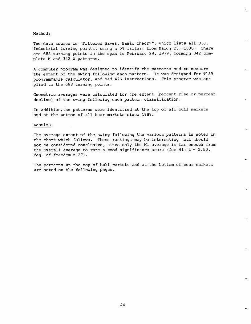
Method:

The data source is "Filtered Waves, Basic Theory", which lists all D.J. Industrial turning points, using a 5% filter, from March 25, 1898. There are 688 turning points in the span to February 28, 1979, forming 342 complete M and 342 W patterns.

A computer program was designed to identify the patterns and to measure the extent of the swing following each pattern. It was designed for T159 programmable calculator, and had 476 instructions. This program was applied to the 688 turning points.

Geometric averages were calculated for the extent (percent rise or percent decline) of the swing following each pattern classification.

In addition,the patterns were identified at the top of all bull markets and at the bottom of all bear markets since 1989.

Results:

The average extent of the swing following the various patterns is noted in the chart which follows. These rankings may be interesting but should not be considered conclusive, since only the Ml average is far enough from the overall average to rate a good significance score (for Ml: t = 2.50, deg. of freedom = 27).

The patterns at the top of bull markets and at the bottom of bear markets are noted on the following pages.

44

(Geometric ovemqes)

Ml6 w3 WI3

WII

,, M4,YIS

t f

” W2 W4

Y8 @ wr w9

‘O

MI4

M3 us YII Yl2

i

I2 t-

Y2

Ml0 Y7 u9

@ = Ove roll Average

9 AAY

I n the pages which follow, n = the number of times the pattern waa found

in the 342 M or 342 W patterns since March 25, 1898.

7’0 rise: this is the percent rise average (geometric) in the swing immediately following an M pattern, or the percent decline in the swing following a W pattern. It is compared with the overall average of all swings,

using a 5% filter.

45

u

m

L#l?iJ-

!!I L

n

l

01

n

H-

5 t

n

5

t

n

~-

c)

N

l L#lTsl- f N

n

WI

0 B 3

n *

l3l-

iz n N

N

*

m-

m 5 n

n

* n

s

Ye

N 0

n N

H-

s In

e

0 N N m- i m v) - E 5

n

Y)

L#lzl-

r 0 N In I.7 0 q - s m N 0 0

m- 2 to 4 N UT I

CD

E

z

N

46

2 I 4 3 5

I

M2 \ \ ? IP

4 I

M3

\ \

% 3 I

3 14 2 5

M4

\ , /1J\. I

Ml n=28 (no.of occurrences: the total for the M patterns is 3.42)

Aver. rise (swing following pattern): 13.89% This is the highest of all the M patterns, and is the only one that has a truly significant difference for the overall average.

Bear market bottoms: This pattern appeared at the end of seven of the fifteen bear markets since 1898. The fifth point of the pattern was the low point of the bear. Is this a confirma- tion of the selling climax idea? It certainly indicates an oversold condition.

Bull market tops: This pattern appears at the top of four bull markets, initiating the new bear with a sharp downtrend.

M2 n=16 Aver. rise: 9.69% This is one of the lowest. Bear market bottoms: two Bull market tops: none

This is a downward zigzag followed by an upward zigzag. These reversals of zigzags have been called "head and shoulders". Several patterns exhibit this reversal.

M3 n= 43 This is the second most popular of the M patterns.

Aver. rise: 9.08% This is below the overall average. Bear market bottoms: four Bull market tops: three (including the 1929 top)

This is a downtrend, but not as steep as Ml.

M4 n= 16 Aver. rise: 11.12% This is close to the average. Bear market bottoms: three Bull market tops: none

This is another reversal from a downward zigzag to an upward zigzag.

3 15 2 4

47

3241 5

M6

325 I4

M7

h \ \ ? 4 I 4 1 325

M5 n=13 Aver. rise: 9.94% This is below average. Bear market bottoms: one Bull market tops: none

This is a "broadening formation". The swings get larger from left to right.

M6 n=6 This one of the rarest of the patterns. Aver. rise: 11.86% This is the third best. Bear market bottoms: one Bull market tops: none

This is a downward zigzag followed by a sharp rise and decline.

M7 n=28 Aver. rise: 9.29% One of the lowest. Bear market bottoms: two Bull market tops: six This is tied with Ml5 for the

most tops.

This pattern begins with a sharp rise followed by a dymward zigzag.

M8 M8 n=4

? I

\

r\r-

Aver. rise: 10.65% This is average. Bear market bottoms: none Bull market tops: none

t This is a wide swing downward zigzag followed by an upward zigzag.

4 I 5 2 3

48

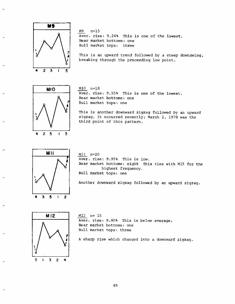
Y9

4 \ t ? 4 I 423 I5

MI0

i I

VP

\ 8

425 I3

MII 1 i I

41” \ \ 4 3 5 I 2

Ml2

&Ic\ Ip # \ \

5 I 3 2 4

M9 n=15 Aver. rise: 9.24% This is one of the lowest. Bear market bottoms: one Bull market tops: three

This is an upward trend followed by a steep downswing, breaking through the preceeding low point.

Ml0 n=18 Aver. rise: 9.55% This is one of the lowest. Bear market bottoms: one Bull market tops: one

This is another downward zigzag followed by an upward zigzag. It occurred recently; March 1, 1978 was the third point of this pattern.

Ml1 n=20 Aver. rise: 9.95% This is low. Bear market bottoms: eight This ties with Ml5 for the

highest frequency. Bull market tops: one

Another downward zigzag followed by an upward zigzag.

Ml2 n= 15 Aver. rise: 9.80% This is below average. Bear market bottoms: one Bull market tops: three

A sharp rise which changed into a downward zigzag.

49

Ml3 ? A

PI I

\ \ 51423

I Ml4

sJ\

? I I \ 1 52314

Ml5

5 24 I3

Ml6

Ml3 n=12 Aver. rise: 12.79% This is the second best of the M

patterns. Bear market bottoms: one Bull market tops: none

This is a triangle with upward breakout.

Ml4 n=24 Aver. rise: 10.12% Bear market bottoms: one Bull market tops: four (including 1929)

This pattern begins with a promising uptrend, but concludes with a bad break.

Ml5 n=44 This is the most frequent of the M patterns. Aver. rise: 11.15% This is close to average. Bear market bottoms: eight This is tied with M 11 for

maximum frequency. Bull market tops: six This is tied with Ml6 for top

frequency.

This pattern occurred recently. February 28, 1979 was the fifth point of this pattern. It's a fine uptrend.

Ml6 n=40 This is the third most frequent. Aver. rise: 11.50% This is the fourth best. Bear market bottoms: four Bull market tops: one

This is a sharp uptrend. Compare it to M15.

50

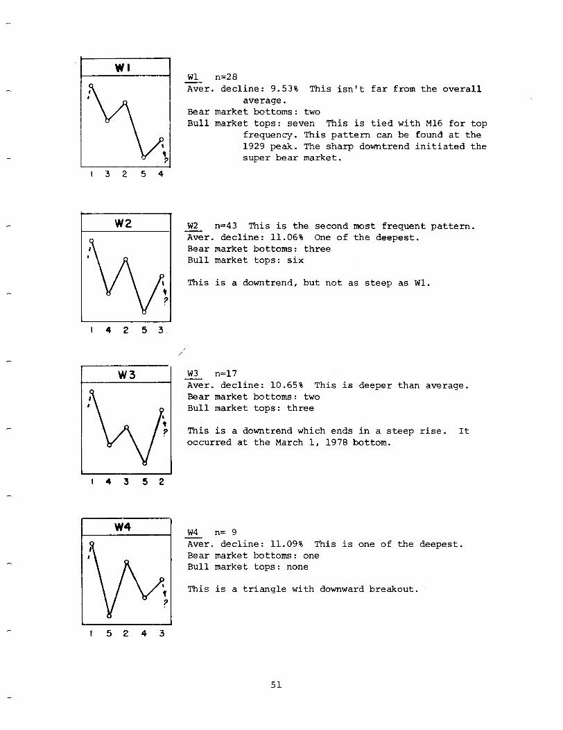
WI

I ,

\2/ \ t ;

I 3 2 5 4

w2

I ,

;/\/

\ c ?

I 4 2 5 3

w3

I I

I t

\2/

7

I4352

Wl n=28 Aver. decline: 9.53% This isn't far from the overall

average. Bear market bottoms: two Bull market tops: seven This is tied with Ml6 for top

frequency. This pattern can be found at the 1929 peak. The sharp downtrend initiated the super bear market.

w2 n=43 This is the second most frequent pattern. Gr. decline: 11.06% One of the deepest. Bear market bottoms: three Bull market tops: six

This is a downtrend, but not as steep as Wl.

/

w3 n=17 Aver. decline: 10.65% This is deeper than average. Bear market bottoms: two Bull market tops: three

This is a downtrend which ends in a steep rise. It occurred at the March 1, 1978 bottom.

I w4 n= 9 Aver. decline: 11.09% This is one of the deepest. Bear market bottoms: one Bull market tops: none

This is a triangle with downward breakout.

I 5 2 4 3

51

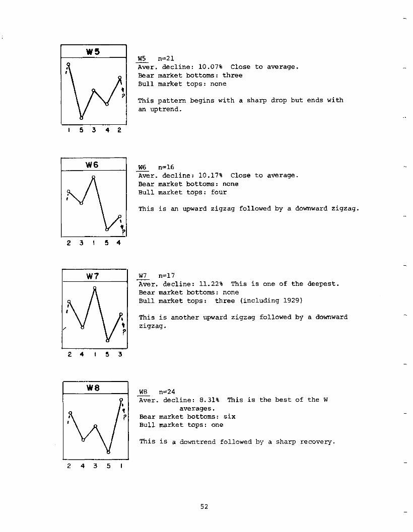
w5 n=21 Gr. decline: 10.07% Close to average. Bear market bottoms: three Bull market tops: none

This pattern begins with a sharp drop but ends with an uptrend.

I 5 3 4 2

W6 W6 n-16 Gr. decline: 10.17% Close to average. Bear market bottoms: none Bull market tops: four

This is an upward zigzag followed by a downward zigzag.

w7

I I

\ik

1 / #

?

24153

w7 n=17 xr. decline: 11.22% This is one of the deepest. Bear market bottoms: none Bull market tops: three (including 1929)

This is another upward zigzag followed by a downward zigzag.

W8 W8 n=24

)A/-

Gr. decline: 8.31% This is the best of the W 1 1 averages.

1 7 Bear market bottoms: six I Bull market tops: one

This is a downtrend followed by a sharp recovery.

2 4 3 5 I

52

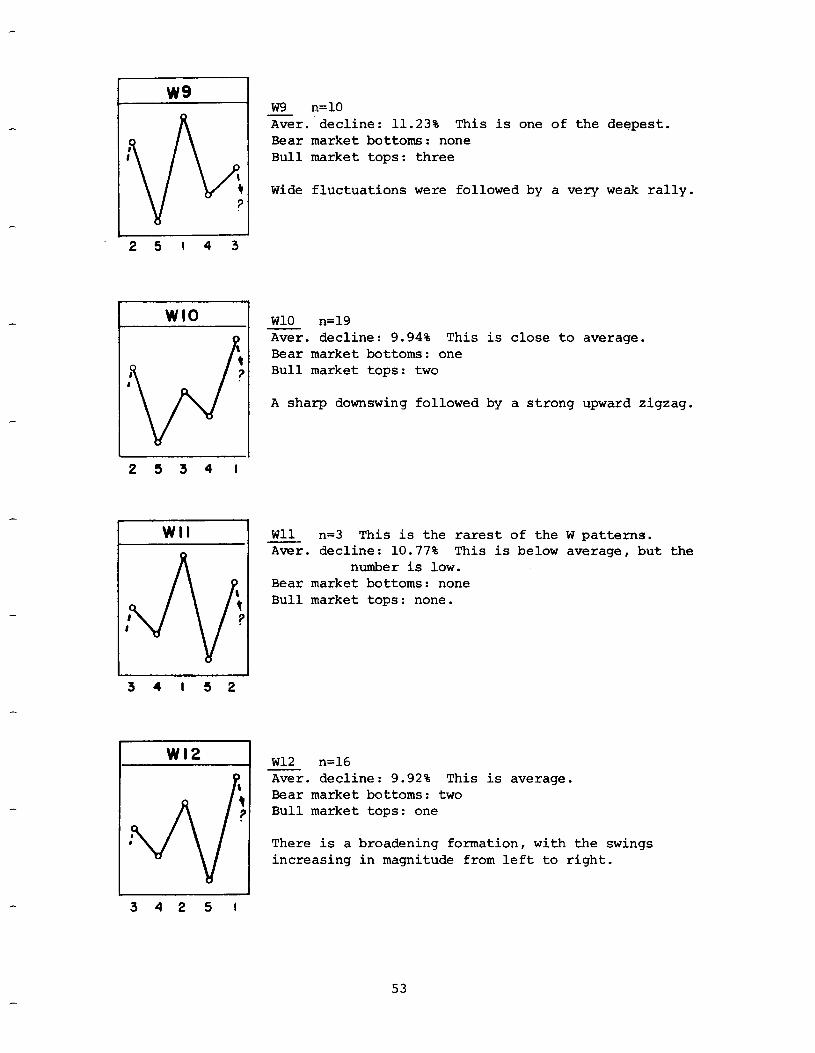
I i- w9 n=lO

A Aver. decline: 11.23% This is one of the deepest. Bear market bottoms: none Bull market tops: three

Wide fluctuations were followed by a very weak rally.

WlO n=19 x. decline: 9.94% This is close to average. Bear market bottoms: one Bull market tops: two

A sharp downswing followed by a strong upward zigzag.

2534 I

Wll n=3 This is the rarest of the W patterns. Aver. decline: 10.77% This is below average, but the

number is low. Bear market bottoms: none Bull market tops: none.

34152

WI2 \ 9 ? 4 :

w12 n=16 Aver. decline: 9.92% This is average. Bear market bottoms: two Bull market tops: one

There is a broadening formation, with the swings increasing in magnitude from left to right.

34251

53

WI3 .-- ___~ I

I

v’l’

c I 3 I

w13 n=22 Aver. decline: 10.54% This is deeper than average. Bear market bottoms: none Bull market peaks: four

This is another upward zigzag followed by a downward zigzag.

3 5 I4 2

WI4

I t

d

?

I I

35241

WIG

45231

w14 n=36 This is the third highest in frequency. Aver. decline: 9.67% This is better than average. Bear market bottoms: two Bull market tops: five

1 This is a fine uptrend. It occurred recently: i March 1, 1978 had this pattern.

w15 n=13 Average decline: 8.47% This is second best. Bear market bottoms: one Bull market tops: two

A strong upward zigzag is followed by a minor downward zigzag.

W16 n=48 This is the most frequent W pattern. Aver. decline: 8.97% This is the third best. Bear market bottoms: seven Bull market tops: seven (including 1929)

This uptrend is steeper than W14.

54

COVERED CALL SWAPPING

Ronald T. Slivka*

As the expiration date of a call option approaches, the manager of a covered call portfolio will want to exchange that option for another with a longer time to expiration. The choices he faces are numerous, for even a single stock will often have a dozen or more different calls available from which to select. To cope with this diversity, rules are frequently adopted to simplify the selection process. For example, a choice is often made to switch to the option having a strike price closest to the current stock price and a time to expiration of about 6 months.

Use of this rule generally assures the new option will possess an adequate time premium for covered call writing and also will have reasonable current liquidity. Such rules, helpful as they may be in coping with diversity of choice, are not always based on calculated economic judgment. It is possible, for example, to improve on such rules by carefully computing the risk and expected return associated with each call option and using the resulting information to determine which call to write. The purpose of this paper is to demonstrate the procedures by which such computations can be made and then utilized to improve portfolio performance.

Covered Call Risk and Return ---

In covered call writing one call is written for each 100 shares of stock owned. The profit and loss profile at the expiration date of option is shown in Figure 1 for this combination of stock and option. The call has an exercise price of E, an initial price, po, and the stock has a future price of x at expiration. The profile of the return on investment (ROI) for the covered call is also shown in Figure 1. As expected, it has a shape very similar to the profit and loss profile. Also shown in Figure 1 is the lognormal probability distribution, p(x), for the future stock price. In this Figure the stock price at the time the call was written is

*Mr. Slivka is Vice President at Morgan Guaranty Trust Company, where he is co-manager of an optioned portfolio of stocks.

55

taken to be E, for convenience. Using this information, we can derive the probability distribution of the return on investment, P(R), shown last in Figure 1. The expected ROI and the standard deviation of ROI can be obtained from this last probability distribution and these two quantities respectively constitute the most conventionally accepted measures of return and risk. For each available option, a risk and return can be calculated and the results arranged for convenience in making investment decisions. It may be seen from this example in Figure 1 that the risk, as defined here, will decrease progressively as the option involved is further in the money. At the same time the dollar return will move lower.

To numerically calculate the risk and return for each stock in the optioned portfolio we begin with the statistical definitions of risk and return:

1. Return = r

P(x) ROI (x) dx = E 0

2. Risk = j/ variance of ROI

3. variance of ROI = /- (ROI(x) - Fj2 P(x) dx 0

One of the most frequently used probability distributions for stock price movement is derived assuming a normal distribution of the variable v, where v is given by

4. v = ln(x/x,) - (r-s2/2)T

SE

x = future stock price

x0 = initial stock price

r = daily growth rate of the stock

S2 = daily variance of the rate of stock price movement

T = time to expiration of call option

All the values required to calculate v are known in advance or are easily obtained from historic stock price data. Numerical values of P(x) are most readily obtained from special computer subroutine programs available on most time-shared computing networks. Some computer subroutines for P(x) are also in the public domain and may be used on in-house computing facil- ities. The ROI profile is easily constructed using the known value of the option at expiration and the initial values of the stock and option prices. The return and risk are then computed by numerical intergration in accord- ance with their definitions as given in equations 1, 2 and 3 above. As complicated as this calculation appears its actual implementation is quite straightforward. A computer program is written to combine all basic information on the stock and options of interest. This program then displays the results of the calculation for use by the portfolio manager.

56

Figure 1

Covered Call Profit C Loss Profile, D(x); ROI Profile, ROI(x);

Stock Price Distribution, P(x); ROI Distribution, P(R)

I D(x)

I I I

ROI(x)

P_(R) I

I E ROI max

57

Covered Call Swapping and Other Uses ---

Displayed in Table I for Boeing are the risk and return results for seven covered calls at the close of business on 12/20/79. These covered calls are listed by ROI from lowest to highest. This rank ordering by ROI makes it possible to locate with minimal difficulty, candidates for call swapping. If, for example, we have an August 50 call in our portfolio we can buy back this call and sell a February 50 picking up about 5% in ROI. For that matter we can swap one option in the list to any other option with a higher ROI. Of course, the addition of commissions into the calculation will reduce all returns leaving the risk values unchanged. Arbitrage candidates similarly can be recognized. For example, the August 50 call canbe arbi- traged against the February 50 or May 50 calls if we wish. The arbitrage, naturally, should yield a positive return after commissions to be considered. Finally, we can use this table to set up spreads. Of critical importance to the profitability of a spread is the degree to which the options involved are overvalued or undervalued. If we wish to set up a diagonal bear spread, for example, we can see immediately from the Table that it is far better to buy an August 50 than a February 50 before selling the Feb- ruary 45.

None of the swapping, arbitrage or spreading strategies can successfully be pursued without including the effects of commission costs and the bid- ask spread. Commission costs are highly variable depending upon the price of the option, the number of option contracts involved, the type of trans- action (swapping, spreading, etc.) and the discounts negotiated with the broker. The complications of a complete commission schedule including all of these effects is best handled by a computer program, for exactness , or by well-tested rules of thumb. In most instances a proper starting point is afforded by inspection of the uniform schedule of commissions in effect prior to May 1, 1975, the date after which commissions were negotiated commissions, discounted 30% from this base schedule appear in Table II along with corresponding option prices. A simple linear relationship exists between the commissions per option (C) and the option price (p) of the form

5. C = 5.272 + 0.9996 p

This relationship makes it easy to compute commissions on trades of about 10 contracts. Similar relationships exist for other quantities of calls traded. In the case where we are swapping 10 February 50s at $5 for 10 May 50s at $6, total commissions on the trades come to approximately $215.40. These commissions reduce the ROI for each option and therefore for the swap as a whole, sometimes making it unattractive. Even if the swap still looks attractive at this point we must make one final adjustment for the bid-ask spread. Prices used in the computation of the ROI in Table I were the average of the bid and ask prices. Execution of the swap may require we buy at the ask and sell at the bid, a spread which may range typically from l/8 to l/2 point. A reasonable estimate of this spread should be used to adjust downward the dollar return resulting from the proposed swap. Following adjustment of the potential swaps for commissions and the bid-ask spread , many fewer candidates remain, as expected.

58

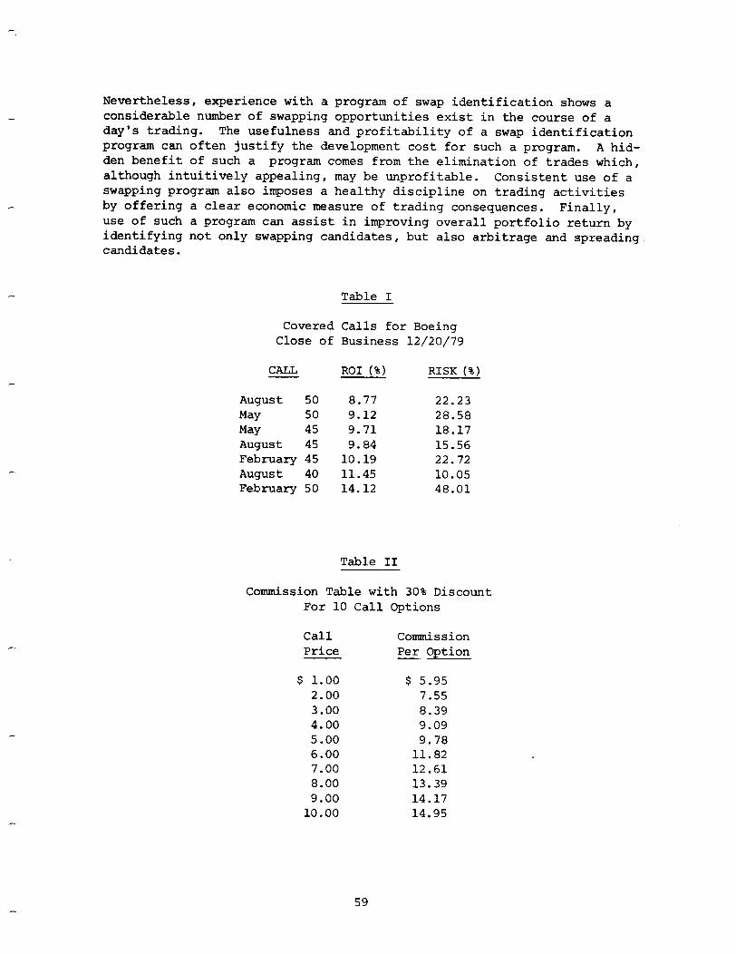
Nevertheless, experience with a program of swap identification shows a considerable number of swapping opportunities exist in the course of a day's trading. The usefulness and profitability of a swap identification program can often justify the development cost for such a program. A hid- den benefit of such a program comes from the elimination of trades which, although intuitively appealing, may be unprofitable. Consistent use of a swapping program also imposes a healthy discipline on trading activities by offering a clear economic measure of trading consequences. Finally, use of such a program can assist in improving overall portfolio return by identifying not only swapping candidates, but also arbitrage and spreading candidates.

Table I

Covered Calls for Boeing Close of Business 12/20/79

CALL ROI (%) RISK (%)

August 50 8.77 22.23 May 50 9.12 28.58 May 45 9.71 18.17 August 45 9.84 15.56 February 45 10.19 22.72 August 40 11.45 10.05 February 50 14.12 48.01

Table II

Commission Table with 30% Discount For 10 Call Options

Call Price

Commission Per Option -.

$ 1.00 $ 5.95 2.00 7.55 3.00 8.39 4.00 9.09 5.00 9.78 6.00 11.82 7.00 12.61 8.00 13.39 9.00 14.17

10.00 14.95

59

intentionally blank

60

Book .

rewews

TECHNICAL ANALYSIS EXPLAINED by Martin J. Pring

Published by McGraw-Hill Book Co. (1980)

Reviewed by: William DiIanni, V.P. Wellington Management Company

The author of this book is Marty Pring who works with the well-known and highly respected advisory service - The Bank Credit Analyst. Marty is also a member of the Market Technicians Association and a good friend. It goes without saying, this book does him and the above organizations proud.

It is quickly apparent that a lot of work went into this book as the author covered the gamut of indicators, methods and theories for the proper understanding of the internal workings of the market. His purpose was directed to knowledge concerning the technical position of the market itself and not the shorter term trading swings and individual stock selection. "The majority of stocks move in sympathy with the overall trend of the market, so an analysis of the macro picture is a good starting point for any serious investment strategy." The book is virtually all inclusive even though some subjects as Dow Theory and Elliott Wave analysis were treated briefly: and as he said, - "left to other books which adequately covered the subject".

The important thing about this book is its comprehensiveness and design. Nearly all methods and indicators of every persuasion have been scrutinized by definition, purpose and construction, with the advantages and disadvan- tages of each. The figures and examples are flawlessly drawn and more than adequate to give the reader a thorough understanding of the matter in question.

Moving from the general to the particular, Marty details trend determination techniques, market structure, interest rates, and other aspects of market behaviour as sentiment and flow of funds indicators. There are 268 pages of well-packed information, and 160 pages of important statistics starting from the year 1790.

As stated before, his coverage of Elliott Wave Principles was brief. Being a student of Elliott Wave Theory myself, I share his caveats but was under- standably disappointed with his cursory treatment of the matter. Marty claims it is too subjective. There may be some truth to this criticism, but the theory does give one a sense of the magnitude of trend and a sense

61

of cyclical expectation. It can prevent one from selling too soon or buying too early. And there is nothing wrong with having a sense of the longevity of sector leadership even though it can be plotted and checked in conventional technical terms. For even Marty admits that "no perfect indicator has ever been developed and one probably never will be". Likewise, the criticism of Elliott in particular is a bit contradictory, since the author says at the outset:

"TO be successful, technical analysis should be regarded as an art, not a science. While many of the mechanistic techniques described in subsequent pages offer reliable indications of changing market conditions, all suffer from the common characteristic that they do sometimes fail to operate satisfacto- rily. This characteristic presents no problem to the con- sciously disciplined investor, since a good working knowledge of the principles underlying major movements in the market, and a balanced view of tis overall technical position, offer a much superior framework within which to operate.

There is, after all, no substitute for independent thought. The action of the technical indicators portrays the underlying characteristics of the market, and it is up to the analyst to put the pieces of the jigsaw puzzle together and come up with a working hypothesis."

Why wouldn't Elliott fit into these paragraphs? Isn't Elliott the ultimate art? (Read Pruden's article in this issue, page 31.)

The epilogue has some very interesting and important principles which we all know and too often forget - I would like to quote the section here:

"At the outset the suggestion was made that the keys to success in the stock market were knowledge and action. The 'knowledge' part of the equation has been discussed as com- prehensively as possible, but the final work has been re- served for investor 'action', since the way in which knowledge is used is just as important as the understanding process itself.

It remains to point out some common errors which all of us commit more often than we would like to. The most obvious of these can be avoided by applying the following principles.

1. Perspective. The interpretation of any indicator should not be based on short-term trading patterns; it should always consider the longer-term implications.

2. Objectivity. A conclusion should not be drawn on the basis of one or two 'reliable' or 'favorite' indicators. The possibility that these indicators could give mis- leading signals demonstrates the need to form a balanced view derived from all available information.

62

3. Humility. One of the hardest lessons in life is learning to admit a mistake. The knowledge of all market partici- pants in the aggregate is, and always will be, greater than that of any one individual or group of individuals. This knowledge is expressed in the action of the market itself as represented by the various indicators. Anyone who 'fights the tape' or the verdict of the market will swiftly suffer the consequences. Under such circumstances, it is as well to become humble and let the mar-

ket give its own verdict; a review of the indicators will frequently suggest its future direction. Occasion- ally the analysis proves to be wrong, and the market fails to act as anticipated. If this unexpected action changes the basis on which the original conclusion was drawn, it is wise to admit the mistake and alter the conclusion.

4. Tenacity. If the circumstances outlined above develop but it is considered that the technical position has not changed, the original opinion should not be changed either.

5. Independent Thought. Should a review of the indicators suggest a position that is not attuned to the majority view, that conclusion is probably well founded. On the other hand, a conclusion should never be drawn simply because it is opposed to that of the majority. In other words, contrariness for its own sake is not valid. Usually the majority conclusion is based on a false assumption, so it is prudent to examine such assumptions to determine their accuracy.

6. Simplicity. Most things done well are also done simply. Because the market operates on common sense, the best approaches to it are basically very simple. If one must resort to complex computer programming and model building, the chances are that the basic techniques have not been mastered and therefore an analytical crutch is required.

7. Discretion. There is a persistent temptation to call every possible market turn, along with the duration of every move the stock market is likely to make. This de- luded belief in one's power to pull off the impossible inevitably results in failure, a loss of confidence, and damage to one's reputation. For this reason, analysis should concentrate on identifying major turning points rather than predicting the duration of a move-for there is no known formula on which consistent and accurate forecasts of this type can be based."

63

In sum, the book is a truly excellent effort to bring under one cover a host of indicators, methods and theories that every technician or market analyst should know. Technical Analysis Explained should definitely be a working handbook for the beginner and the professional alike - for a periodic review of the basics is always important and helpful for everyone.

But as with everything else in life, the implementation will always depend on the insights and genius of the user. There is always a danger of getting lost in the tools themselves. Hence, proper use of this technical arsenal rests in a proper synthesis after years of experience over many market cycles.

As for subjectiveness - it is not always bad. The only things in life devoid of subjectivity are simple arithmetic, as 2 + 2 = 4; and perhaps, the first principles in philosophy.

We all look forward with eager anticipation to the other books Marty is writing. Meantime, this book is a must!

64

intentionally blank

65

intentionally blank

66

journal of technical analysis (jota). issue 07 (1980, february)

Economy & Finance

mta journal

mta meetings

stock market strategy

annual seminar fee

following mta members

monthly mta newsletter

new jersey

indicator analysis