journal of theoretical biology - uni-freiburg.de

Journal of Theoretical Biology 335 (2013) 222–234

Contents lists available at SciVerse ScienceDirect

Journal of Theoretical Biology

0022-51http://d

n Corrof Edinb

E-m

journal homepage: www.elsevier.com/locate/yjtbi

Signatures of nonlinearity in single cell noise-induced oscillations

Philipp Thomas a,b,c, Arthur V. Straube c, Jens Timmer d, Christian Fleck f,g, Ramon Grima a,e,n

a School of Biological Sciences, University of Edinburgh, United Kingdomb School of Mathematics, University of Edinburgh, United Kingdomc Department of Physics, Humboldt University of Berlin, Germanyd BIOSS Centre for Biological Signalling Studies, University of Freiburg, Germanye Freiburg Institute for Advanced Studies, University of Freiburg, Germanyf Laboratory for Systems and Synthetic Biology, Wageningen University, Netherlandsg Centre for Biological Systems Analysis (ZBSA), University of Freiburg, Germany

H I G H L I G H T S

� We develop a general theory of noise-induced oscillations in subcellular volumes.
� The theory provides the power spectrum in closed form for any monostable network.� The spectra close to a Hopf bifurcation have three universal features.� The predicted features are seen in experimental single cell data.� Simulations of circadian and mitotic oscillators verify the theory's accuracy.
a r t i c l e i n f o

Article history:Received 10 January 2013Received in revised form20 May 2013Accepted 18 June 2013Available online 2 July 2013

Keywords:Master equationsStochastic differential equationsOscillationsLinear noise approximationIntrinsic noise

93/$ - see front matter & 2013 Elsevier Ltd. Ax.doi.org/10.1016/j.jtbi.2013.06.021

esponding author at: C. H. Waddington Buildiurgh, EH9 3JD, UK. Tel.: +44 131 651 9060.ail address: [email protected] (R. Grima

a b s t r a c t

A class of theoretical models seeks to explain rhythmic single cell data by postulating that they aregenerated by intrinsic noise in biochemical systems whose deterministic models exhibit only dampedoscillations. The main features of such noise-induced oscillations are quantified by the power spectrumwhich measures the dependence of the oscillatory signal's power with frequency. In this paper we derivean approximate closed-form expression for the power spectrum of any monostable biochemical systemclose to a Hopf bifurcation, where noise-induced oscillations are most pronounced. Unlike the commonlyused linear noise approximation which is valid in the macroscopic limit of large volumes, our theory isvalid over a wide range of volumes and hence affords a more suitable description of single cell noise-induced oscillations. Our theory predicts that the spectra have three universal features: (i) a dominantpeak at some frequency, (ii) a smaller peak at twice the frequency of the dominant peak and (iii) a peak atzero frequency. Of these, the linear noise approximation predicts only the first feature while theremaining two stem from the combination of intrinsic noise and nonlinearity in the law of mass action.The theoretical expressions are shown to accurately match the power spectra determined from stochasticsimulations of mitotic and circadian oscillators. Furthermore it is shown how recently acquired single cellrhythmic fibroblast data displays all the features predicted by our theory and that the experimentalspectrum is well described by our theory but not by the conventional linear noise approximation.

& 2013 Elsevier Ltd. All rights reserved.

1. Introduction

Cellular rhythms are ubiquitous throughout many tissues of thebody (Mohawk et al., 2012). The central pacemaker of themammalian circadian clock located in the suprachiasmatic nucleusis thought to be entrained to a light-dark cycle and to reset the

ll rights reserved.

ng, Mayfield Road, University

).

expression of clock genes in peripheral tissues in vivo (Mohawket al., 2012). For example, 10% of the transcriptome and 20% of theproteome in mouse liver are expressed rhythmically (Panda et al.,2002; Reddy et al., 2006). Similar fractions have been found to beunder circadian control in the human metabolome indicating thatrhythmic expression of clock genes controls many downstreampathways (Dallmann et al., 2012).

In the absence of pacemaker control, isolated peripheral clocksfunction as sustained but independently phased cell autonomous24 h-oscillators under constant light conditions (Welsh et al.,2004; Nagoshi et al., 2004). In consequence initially synchronized

www.sciencedirect.com/science/journal/00225193

www.elsevier.com/locate/yjtbi

http://dx.doi.org/10.1016/j.jtbi.2013.06.021



http://crossmark.dyndns.org/dialog/?doi=10.1016/j.jtbi.2013.06.021&domain=pdf



mailto:[email protected]


days

02468

0 5 10 15 20 2502468

0 5 10 15 20 25

0 5 10 15 20 2502468

0 5 10 15 20 2502468

days

luminescence

Fig. 1. Single cell circadian oscillations in individual fibroblast cells over two weeks after medium change reproduced from experimental dataset S1 in Leise et al. (2012).(a–c) Single time course of protein luminescence of first three individual fibroblast cells shows sustained oscillations. (d) Population average over the first 20 cells shows adampening of the oscillations due to dephasing of individual cell rhythms.

P. Thomas et al. / Journal of Theoretical Biology 335 (2013) 222–234 223

cell cultures display only damped oscillations on the ensemblelevel due to a gradual dephasing of individual cellular clocks(Welsh et al., 2004; Westermark et al., 2009). Fig. 1 illustrates thisphenomenon by comparing three time traces of protein lumines-cence (a–c) from single fibroblast cells against the averagedresponse of a culture of 20 cells shown in (d). The images havebeen reproduced from dataset S1 in Leise et al. (2012).

It is still under debate what is the underlying single cellmechanism responsible for producing oscillations. In the absenceof noise, populations of synchronized self-sustained oscillatorsexhibit in-phase oscillations of constant amplitude while popula-tions of damped oscillators show an in-phase decaying amplitude.In both cases, taking into account the molecular fluctuationsstemming from the stochastic nature of the underlying biochem-ical reactions leads to a population of cells with sustained (noisy)oscillations and with cell-to-cell variation in the phase. Hencepresently experimental single cell data can be explained by bothnoisy self-sustained and damped oscillator models (Westermarket al., 2009).

The fact that molecular noise induces a deterministicallydamped oscillator to exhibit sustained oscillations has led to thisphenomenon being called noise-induced oscillations (NIOs) (Vilaret al., 2002; McKane et al., 2007). The amplitude of theseoscillations is proportional to 1=

ffiffiffiffiN

pwhere N is the mean number

of molecules. Hence NIOs have been deemed important forreactions involving a typically small number of molecules suchas those occurring inside cells (Grima and Schnell, 2008). Similarmechanisms to generate NIOs have been described as coherenceresonance with non-excitable dynamics in the contexts of epi-demics (Kuske et al., 2007), predator–prey interactions (Rozenfeldet al., 2001) and lasers models (Ushakov et al., 2005).

The power spectrum of concentration fluctuations has been themain measure used to quantify NIOs, both experimentally andtheoretically, to date (Gang et al., 1993; Hou and Xin, 2003; Welshet al., 2004; Davis and Roussel, 206; Li and Lang, 2008; Geva-Zatorsky et al., 2010; Ko et al., 2010). Briefly speaking the powerspectrum measures how the square amplitude of a signal isdistributed with frequency. In particular, peaks in the powerspectrum indicate the presence of NIOs. For systems composedof purely first-order reactions, exact expressions for the powerspectrum of concentration fluctuations can be derived from thechemical master equation (CME) (the accepted mesoscopicdescription of biochemical kinetics) (Warren et al., 2006;Simpson et al., 2004). However, most biochemical systems ofinterest do not fall in the latter category since they are composedof a large number of bimolecular reactions arising from oligomerbinding, cooperativity, allostery or phosphorylation of proteins(Novák and Tyson, 2008). A popular means to obtain approximateexpressions for the power spectra of systems composed of both

unimolecular and bimolecular reactions is the linear noise approx-imation (LNA) of the CME (Van Kampen, 1976; Dauxois et al., 2009;McKane et al., 2007; Qian, 2011; Toner and Grima, 2013) wherebythe probability distribution solution of the CME is approximatedby a Gaussian. It is, however, the case that the LNA provides a goodapproximation to the CME only in the limit of large volumes atconstant concentrations, i.e., the limit of large molecule numbers.Given that molecule numbers of several key intracellular playersare in the range of few tens to several thousands (Schwanhäusseret al., 2011), it is plausible that the predictions of the LNA maybelimited in scope for biological systems. Indeed recent studies(Grima, 2009, 2010, 2012; Thomas et al., 2010; Ramaswamyet al., 2012) have shown that the mean concentrations andvariances of interacting chemical species present in low moleculenumber can be considerably different than those given by the LNA;these effects originate from the combination of intrinsic noise andnonlinearity in the law of mass action. Similarly analytical studiesof two-variable epidemic (Chaffee and Kuske, 2011) and predator–prey models (Scott, 2012) revealed NIOs with more than onefrequency that are not captured by linear analysis. While it is clearthat the LNA must miss some of the crucial features of single cellNIOs, athorough investigation of these effects has not been carriedout to-date.

In this paper we obtain the leading order correction to theLNA's prediction of the power spectrum of the fluctuations for ageneral biochemical reaction pathway whose corresponding deter-ministic system is just below a super-critical Hopf bifurcation. Weshow that this novel nonlinear contribution to the power spec-trum yields additional peaks at zero frequency and at twice thefrequency of the peak predicted by the LNA. The analytical resultsare verified by comparison with experimental single cell data ofrhythmic fibroblast cells and with detailed stochastic simulationsof an oscillator controlling mitosis and of a transcriptional feed-back oscillator.

2. Preliminaries: linear theory of noise-induced oscillations

2.1. The standard description of stochastic chemical kinetics

We consider a general chemical system consisting of a numberN of distinct chemical species interacting via R chemical reactionsof the type

s1jX1 þ⋯þ sNjXN-kjr1jX1 þ⋯þ rNjXN ð1Þ

occurring in a volume of mesoscopic size Ω. Here j is an indexrunning from 1 to R, Xi denotes chemical species i, sij and rij are thestoichiometric coefficients and kj is the rate constant of the jthreaction. Under well-mixed conditions there are two descriptions

P. Thomas et al. / Journal of Theoretical Biology 335 (2013) 222–234224

that have been commonly employed to describe such systems. Inthe first approach the time-dependent concentrationsϕ¼ ðϕ1;…;ϕNÞT are obtained from the solution of deterministicrate equations (REs):

∂∂t

ϕ¼ f ðϕÞ: ð2Þ

In the second approach the mesoscopic state is given by a vector ofpopulation numbers n¼ ðn1;…;nNÞT drawn from a probabilitydistribution. The time evolution equation of this probabilityΠðn; tÞ is given by the CME (Gillespie, 2007; van Kampen, 2007):

∂Πðn; tÞ∂t

¼ ∑R

j ¼ 1ðajðn�μjÞΠðn�μj; tÞ�ajðnÞΠðn; tÞÞ: ð3Þ

where ajðnÞdt is the probability that the jth reaction occurs withininfinitesimal time dt and the state n changes to nþ μj whereμj ¼ ðr1j�s1j; r2j�s2j;…; rNj�sNjÞ. Following Gillespie (2007) we shallrefer to μj as the state-change vector for the jth reaction. It hasbeen shown that the relation between the functions f and thepropensities aj is given by the macroscopic limit f ðϕÞ ¼ limΩ-1∑jμjajðΩϕÞ=Ω in which both descriptions, Eqs. (2) and (3), areequivalent (van Kampen, 2007; Thomas et al., 2012). It is, however,well appreciated that this limit does not accurately capture thedynamics of biochemical reactions in individual cells but ratherresembles more closely the average over populations ofidentical cells.

The discrepancy between the two approaches stems from thefact that the deterministic approach assumes the molecule num-bers in a cell to be sufficiently large while the stochastic onesuffers no such restriction. A popular method to simulate stochas-tic time traces distributed according to the solution of Eq. (3) is thestochastic simulation algorithm (SSA) as introduced by Gillespie.Such simulations are widely used to show off qualitative devia-tions from the deterministic description such as the existence ofnoise-induced oscillations which were indeed observed in Gilles-pie's seminal paper introducing the SSA (Gillespie, 1977).

As mentioned in the Introduction, NIOs are quantified bymeans of the power spectrum of concentration fluctuations. Thisis formally defined as follows. The autocorrelation function of thesth species is given by

ΣsðτÞ ¼ nsðtÞ�⟨ns⟩Ω

� �nsðt þ τÞ�⟨ns⟩

Ω

� �� ; ð4Þ

which allows to identify periodicities present in individual realiza-tions ns(t) of the stochastic process. Note that the angled bracketsdenote the ensemble average and t is any time for which thesystem has achieved steady-state. The power spectral density offluctuations is then defined by the Fourier transform of theautocorrelation function

PsðωÞ ¼Z 1

�1dτ e�iωτΣsðτÞ; ð5Þ

such that PsðωÞdω=ð2πÞ is the power contained in the infinitesimalfrequency interval dω=ð2πÞ. For brevity we refer to Eq. (5) simply asthe power spectrum of the concentration fluctuations of species s.

2.2. Power spectra within the linear noise approximation

While the power spectrum Eq. (5) is easy to obtain experimen-tally or to calculate from stochastic simulations using the SSA, it isnot generally possible to obtain exact expressions for it unless thesystem is composed of only unimolecular reactions (Warren et al.,2006). The use of the LNA bypasses this difficulty, and we nextbriefly review this approach (for more details see the sectionMethods).

The LNA has been derived by van Kampen using the system sizeexpansion (van Kampen, 2007) and has been subsequently exten-sively used to quantify NIOs by others. The LNA result states that inthe limit of large molecule numbers, the fluctuating concentrationpredicted by the CME for a single cell is approximately equal to asum of two terms: a contribution describing the populationaverage ϕðtÞ given by the REs, Eq. (2), and another contributiondescribing fluctuations ϵðtÞ about them in a single cell:

nðtÞΩ

¼ϕðtÞ þ ϵðtÞ; ð6Þ

where the time-evolution of the fluctuations ϵðtÞ is given by thelinear Langevin equation

ddt

ϵðtÞ ¼ JðϕðtÞÞϵðtÞ þΩ�1=2BðϕðtÞÞΓðtÞ; ð7Þ

where the matrix J denotes the Jacobian of the deterministicequation, Eq. (2), the elements of the matrix B readBij ¼Ω�1=2μij

ffiffiffiffiffiffiffiffiffiffiffiffiffiffiajðΩϕÞp

where μij is the ith component of the vectorμj and the R-dimensional vector Γ is Gaussian white noise satisfy-ing ⟨ΓiðtÞΓjðt′Þ⟩¼ δijδðt�t′Þ for each pair of reactions. Note thatunderlined symbols represent matrices throughout the paper.Note also that our notation is slightly different than the one usedby van Kampen where the quantity ϵðtÞ has been rescaled by afactor of Ω1=2 (see van Kampen, 2007, Chapter X).

It can be shown by taking the Fourier transform of Eq. (7) thatthe power spectrum of fluctuations in species s is given by

PLNAs ðωÞ ¼ 1

Ω½ðJ�iωÞ�1BBT ðJT þ iωÞ�1�ss; ð8Þ

which can be more usefully written using the eigenrepresentationof the Jacobian

PLNAs ðωÞ ¼ 1

Ω∑ijU�1

si

½ ~B ~B† �ij

ðλi�iωÞðλnj þ iωÞU�†js ; ð9Þ

where U�1 is the matrix of eigenvectors of J and the λ's are itseigenvalues, as given by the relationship UJU�1 ¼ diagðλ1; λ2;…; λNÞ.The matrix ~B is defined as equal to UB. Note that U�† is shorthandnotation for ðU�1Þ†. By inspection of the above equation one candeduce that when there exists a pair of complex conjugate eigenva-lues the dependence of the denominator can yield a Lorentzian peakat a nonzero frequency which is the signature of a NIO (McKane et al.,2007).

In what follows we assume that the eigenvalue spectrum ofthe Jacobian J is composed of a pair of conjugate eigenvaluesλ1 ¼�γ þ iω0, λ2 ¼�γ�iω0 and N�2 real negative eigenvalues λiwhere i¼ 3;…;N. The deterministic dynamics then corresponds toa focus which becomes unstable as γ-0, i.e., the Hopf bifurcationpoint. In particular, by considering the dominant term in Eq. (9)(corresponding to i¼ j¼ 1), one can deduce that the powerspectrum has a peak at ω≈ω0 wheneverγ

ω051; ð10Þ

i.e., the phenomenon of NIO becomes particularly conspicuouswhen the deterministic dynamics is close to a critical point givingrise to a limit cycle through a Hopf bifurcation (Ushakov et al.,2005). In this case the total power is concentrated in the peak andcan be approximated by the peak height ð∼G=ðΩγ2ÞÞ, whereG¼ ½ ~B ~B

†�11, multiplied by its spectral width ð∼γÞ, is of the order

GΩγ

: ð11Þ

Since the total power is equal to the variance of the NIO it followsthat Eq. (11) needs to be sufficiently small for the LNA to hold.Similar criteria have been obtained using multiple scale analysis inKuske et al. (2007) (see Eq. (24) therein). In the same limit the


sample paths of Eq. (7) can be interpreted as given by a fast oscillationwith frequency ω0 whose amplitude is stochastically modulated onthe slow timescale 1=γ (Baxendale and Greenwood, 2011).

3. Results: nonlinear theory of noise-induced oscillations

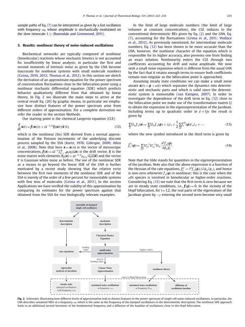
Biochemical networks are typically composed of nonlinear(bimolecular) reactions whose stochastic kinetics is not accountedfor insufficiently by linear analysis; in particular the first andsecond moments of intrinsic noise as given by the LNA becomeinaccurate for nonlinear systems with small molecule numbers(Grima, 2010, 2012; Thomas et al., 2012). In this section we sketchthe derivation of an approximate equation for the power spectrumof concentration fluctuations close to the bifurcation point using anonlinear stochastic differential equation (SDE) which predictsbehavior qualitatively different from that obtained by lineartheory. In Fig. 2 we illustrate the main steps to arrive at thecentral result Eq. (20) by graphic means, in particular we empha-size how distinct features of the power spectrum arise fromdifferent orders of approximation. For a complete derivation werefer the reader to the section Methods.

Our starting point is the chemical Langevin equation (CLE)

ddt

xðtÞ ¼ f ðxðtÞÞ þΩ�1=2BðxðtÞÞΓðtÞ; ð12Þ

which is the nonlinear (Ito) SDE derived from a normal approx-imation of the Poisson increments of the underlying discreteprocess sampled by the SSA (Kurtz, 1976; Gillespie, 2000; Allenet al., 2008). Note that here x¼ n=Ω is the vector of mesoscopicconcentrations, f ðxÞ ¼Ω�1∑R

j ¼ 1μjajðΩxÞ is the drift vector, B is thenoise matrix with elements BijðxÞ ¼Ω�1=2μij

ffiffiffiffiffiffiffiffiffiffiffiffiffiffiajðΩxÞp

and the vectorΓ is Gaussian white noise as before. The use of the nonlinear SDEas a means to go beyond the linear SDE of the LNA is furthermotivated by a recent study showing that the relative errorbetween the first two moments of the nonlinear SDE and of theSSA is merely of the order of a few percent for monostable systemswith few tens of molecules (Grima et al., 2011). In the sectionApplications we have verified the validity of this approximation bycomparing its estimates for the power spectrum against thatobtained from the SSA for two biologically relevant examples.

Fig. 2. Schematic illustrating how different levels of approximation lead to distinct featuLNA describes sustained NIOs at a frequency ω0 which is the same as the frequency of thleads to an additional second harmonic of the fundamental frequency and a diffusion o

In the limit of large molecule numbers (the limit of largevolumes at constant concentration), the CLE reduces to theconventional deterministic REs given by Eq. (2) and the LNA, Eq.(7), accounting for the fluctuations (Grima et al., 2011; Wallaceet al., 2012). As previously mentioned, for intermediate moleculenumbers, Eq. (12) has been shown to be more accurate than theLNA, however, the nonlinear character of the equation which isresponsible for its higher accuracy, also prevents one from findingan exact solution. Nonlinearity enters the CLE through twocoefficients accounting for drift and noise amplitude. We nowseek a small noise expansion which is different from the usual LNAby the fact that it retains enough terms to ensure both coefficientsremain non-singular as the bifurcation point is approached.

Assuming steady state conditions we can make a small noiseansatz xðtÞ ¼ ϕþ ϵðtÞ which separates the dynamics into determi-nistic and stochastic parts and which is valid since the determi-nistic system is monostable (van Kampen, 2007). In order toinvestigate the dependence of the drift term in Eq. (12) close tothe bifurcation point we make use of the transformation matrix Uto obtain the expansion in the eigenrepresentation of the Jacobian.Including terms up to quadratic order in ~ϵ ¼Uϵ the result isgiven by

∑αUiαf αðxÞ ¼∑

αUiαf αðϕÞ þ λi ~ϵ i þ

12∑αβ

~Jαβ

i ðϕÞ~ϵα ~ϵβ þ⋯ ð13Þ

where the new symbol introduced in the third term is given by

~Jrsi ðϕÞ ¼ ∑

αμνU�1

μr U�1νs Uiα

∂2f αðϕÞ∂ϕμϕν

: ð14Þ

Note that the tilde stands for quantities in the eigenrepresentationof the Jacobian. Note also that the above expression is a function ofthe Hessian of the rate equations, Jμνα ¼ ∂2f αðϕÞ=ð∂ϕμ∂ϕνÞ, and henceis non-zero whenever f αðϕÞ is nonlinear; this is the case when theαth species is involved in bimolecular or higher-order reactions.Considering Eq. (13) we note that the first term is zero because weare in steady state conditions, i.e., f ðϕÞ ¼ 0. In the vicinity of theHopf bifurcation, for i¼1,2, the real parts of the eigenvalues of theJacobian given by �γ entering the second term become very small

res in the power spectrum of single cell noise-induced oscillations. In particular, thee damped oscillations in the deterministic description. The nonlinear SDE approachf the baseline of oscillations close to the Hopf bifurcation.


and hence the real parts of the third term dominate. Thus up tosecond-order terms must be retained to guarantee that the driftcoefficient is not singular as the bifurcation point is approached. Incontrast, for the noise coefficient the leading order contribution issufficient since the first term in its expansion, ~BiαðϕÞ is non-zero atthe bifurcation. Hence using the eigenrepresentation of the Jaco-bian the nonlinear Langevin equation, Eq. (12), can be approxi-mated as

∂t ~ϵiðtÞ ¼ λi ~ϵi þ12∑αβ

~Jαβ

i ðϕÞ~ϵα ~ϵβ þΩ�1=2∑α

~BiαðϕÞΓαðtÞ; ð15Þ

close to the bifurcation point. Still, the power spectrum of theabove Langevin equation cannot be obtained straightforwardlysince the nonlinear character of the equation is retained and henceto proceed further an approximation method becomes indispen-sable. We now substitute the Fourier transform

~ϵ iðtÞ ¼Z 1

�1

dω2π

eiωt ϵ̂ iðωÞ; ð16Þ

into Eq. (15) and expand ϵ̂ i in powers of the inverse square root ofthe system size

ϵ̂ iðωÞ ¼Ω�1=2ϵ̂ð0Þi ðωÞ þΩ�1ϵ̂ð1Þi ðωÞ þ OðΩ�3=2Þ: ð17Þ

After equating terms of order Ω�1=2 and subsequently those oforder Ω�1 one finds that the power spectrum of the sth speciesexpressed in the eigenrepresentation of the Jacobian is given by

PsðωÞ ¼ PLNAs ðωÞ

þ 1Ω2 U

�1ð⟨ϵ̂ð1ÞðωÞϵ̂ð1Þ†ðωÞ⟩�δðωÞ⟨~ϵð1Þ⟩⟨~ϵð1ÞT⟩ÞU�† ; ð18Þ

where the first term is related to the spectrum of ϵ̂ð0Þi ðωÞ byPLNAs ðωÞ ¼U�1⟨ϵ̂ð0ÞðωÞϵ̂ð0Þ†ðωÞ⟩U�† and is exactly equivalent to Eq.

(9) obtained by the LNA while the second is a correction termrelated to the spectrum of ϵ̂ð1Þi ðωÞ accounting for nonlinear effectsin Langevin equation (15).

As shown in the Methods section, Eq. (18) simplifies to

PsðωÞ ¼1Ω∑ijU�1

si

½ ~B ~B† �ij

ðλi�iωÞðλnj þ iωÞU�†js

� 12Ω2 ∑

ij∑αβμν

U�1si

~Jαβ

i ~sαμ

ðλi�iωÞ1

λα þ λβ�iωþ 1

λnμ þ λnν þ iω

!

�~Jnμν

j ~snνβ

ðλnj þ iωÞU�†js þ OðΩ�5=2Þ; ð19Þ

where ~sij ¼�½ ~B ~B†�ij=ðλi þ λnj Þ is the LNA covariance matrix of the

eigenmodes. The above expression is the spectrum of the non-linear Langevin equation (15) accurate to order Ω�2. The latter aswe have argued approximates the CME in the limit of largepopulation numbers close to the Hopf bifurcation point. In theMethods section we have shown that close to the bifurcation,the covariance of the near-critical eigenmodes is diagonallydominant, i.e., ~s ij≃δijG=ð2γÞ (for i and j equal to 1 or 2) withG¼ ½ ~B ~B

†�11 ¼ ½ ~B ~B†�22 and hence these yield the major contribu-

tions to the sum. Given this reasoning we can write the powerspectrum of the concentration fluctuations of species s close to thebifurcation:

PsðωÞ≈PLNAs ðωÞ þΩ�2G2

2γjM11

s ðωÞj2ðω�2ω0Þ2 þ ð2γÞ2

þ 2jM12

s ðωÞj2ω2 þ ð2γÞ2

!; ð20Þ

where non-resonant contributions have been omitted. The coeffi-cients in the above expression are given by

Mijs ðωÞ ¼ ∑

αμν½ðJ�iωÞ�1�sαU�1

μi U�1νj

∂2f αðϕÞ∂ϕμ∂ϕν

: ð21Þ

The first term in Eq. (20) is the prediction of the LNA whichleads to a peak at ω≃ω0. Specifically, the second term in Eq. (20)leads to a peak at twice the LNA frequency ω≃2ω0, and the thirdterm leads to a peak at zero frequency ω≃0 whenever we are closeto the Hopf bifurcation point. These extra peaks are due to thecombined influence of noise and nonlinearity of the chemicalreactions. As argued in the previous section the fundamental peakgives a contribution of order G=ðΩγÞ to the overall variance;similarly it can be shown that the total power concentrated inthe additional two peaks is of order

GΩγ

� �2

: ð22Þ

It hence follows that the corrections in Eq. (20) become significantwhen G=Ω≃γ, i.e., when there exists a balance between thenoise coefficient G=Ω and the distance from the bifurcationpoint γ. The conditions for the observability of the additionalpeaks at twice the frequency of the principal peak and at zerofrequency require

jM11s ð2ω0Þj≠0; jM12

s ð0Þj≠0; ð23Þ

respectively. Using the above together with Eq. (21) it follows thatthe Hessian of the corresponding deterministic system ∂2f αðϕÞ=ð∂ϕμ∂ϕνÞ needs to be non-zero at the bifurcation point; however,this condition is not sufficient. Assuming that jM11

s ð2ω0Þj is acontinuous function of ω0 then clearly the first condition in Eq.(23) is fulfilled for all values of 2ω0 except the zeros of M11

s whichdepend on the specific rate constants of the network underconsideration. The second condition in Eq. (23) is independent ofω0 and is as we show in the next section not generally true for allbiochemical processes of interest.

The physical meaning of the peak at zero frequency is not asintuitive as the peaks at non-zero frequency and requires furtherexplanation. Given that γ is very small (since we are close to theHopf bifurcation) and assuming that M12

s ð0Þ≠0 then it follows thatthe spectrum associated with the last term on the right hand sideof Eq. (20) is approximately proportional to jM12

s ð0Þj2ω�2 forω0⪢ω⪢γ. A spectrum characterized by this scaling form is asso-ciated with random walk noise; to be more precise, given aLangevin equation ∂txðtÞ ¼

ffiffiffiffiffiffiffi2D

pΓðtÞ where D is the diffusion

coefficient and ΓðtÞ is white noise, then the power spectrum ofthe signal x(t) is equal to 2D=ω2. Thus it follows that the fluctuat-ing signal whose spectrum is given by Eq. (20) can be interpretedas the sum of the three components: (i) a component whichfluctuates about the mean with diffusion coefficient jM12

s ð0Þj2G2=

ð2Ω2γÞ; (ii) a noisy component with power concentrated at afrequency of ω0; (iii) another oscillatory component as (ii) butwith power concentrated at a frequency of 2ω0. These componentsare, respectively, associated with the spectra given by the lastterm, the first term and the second term on the right hand side ofEq. (20). We also note that the integral of Eq. (20) over ω gives thevariance of the fluctuations in species s close to the bifurcation;this is a sum of the variance predicted by the LNA and a correctionterm of order Ω�2. The latter is always positive and hence it can bestated that to the order of the approximation used, the LNAinvariably underestimates the variance close to a Hopf bifurcation.

In the next section we apply our theory to the three cases ofbiological interest. In particular we show how the theory can beused to explain recently obtained experimental single cell rhythmdata and also illustrate by means of two examples how onecalculates Eq. (20) for a given system of interest. Stochasticsimulations using the SSA are used to verify the accuracy of ourtheory for intermediate volumes and also to probe small volumephenomena which are beyond its predictive power.


4. Applications

4.1. Noise-induced oscillations observed in individual fibroblast cells

Recently, Leise et al. (2012) reported experimental proteinluminescence data from cultures of 80 highly rhythmic fibroblastcells. Single cell spectra were obtained from individual observa-tions over a six week period and averaged over the cell population.This data (see dataset S1; also shown in Leise et al. (2012, Fig. 6(b))has the main features predicted by our theory, namely a peak atzero frequency, a dominant peak at the circadian frequency and asecond harmonic. We therefore investigate if the experimentaldata can be fit by our proposed theoretical expression for thepower spectrum, Eq. (20). Our strategy is as follows: (i) wepropose a biologically plausible network motif explaining theobserved oscillatory single cell dynamics, (ii) we fit the principalpeak of the experimental power spectrum using the LNA for thismotif and (iii) we refine our fit by taking into account theadditional peaks in the spectrum using our main result, Eq. (20),applied to the motif.

The ability of biological systems to oscillate is often associatedwith the presence of a negative feedback loop in the underlyingbiochemical network (Novák and Tyson, 2008). Given the fact thatany biochemical oscillator must be composed of at least threecomponents we propose a negative feedback motif involvingmRNA (M) and two forms of a protein (P and Pn) as a candidatefor explaining the experimental rhythmic fibroblast data (see Fig. 3(a) for an illustration). The dynamics for this motif could forexample be deterministically described by the set of coupled rateequations

∂tϕM ¼ k0k1 þ ϕP

�α1ϕM ; ð24Þ

∂tϕPn ¼ β1ϕM�α2ϕPn ; ð25Þ

∂tϕP ¼ β2ϕPn� k2ϕP

k3 þ ϕP; ð26Þ

where ϕM , ϕPn and ϕP are the concentrations of mRNA and the twoproteins. The Jacobian for these rate equations is given by

J ¼�α1 0 �χ

β1 �α2 00 β2 �α3

0B@

1CA; ð27Þ

where α1;2;3, β1;2 and χ are positive constants. Note that χ measuresthe strength of the negative feedback loop and is equal tok0=ðk1 þ ϕPÞ2 whereas α3 is a measure of the nonlinear protein

Fig. 3. Least squares fit of the experimental power spectrum of circadian rhythm in fibroexplaining the single cell dynamics observed in Leise et al. (2012). (b) Fit of the experimeand by the proposed nonlinear theory (magenta solid line) is shown. Note that the LNA cand at a second harmonic frequency. The nonlinear theory is in excellent quantitativtheoretical curves are given in the main text. (For interpretation of the references to co

degradation rate and is equal to k2k3=ðk3 þ ϕPÞ2. Indeed it can beshown that this is a generic form for the Jacobian of all negativefeedback motifs with three components (Tyson, 2002). The onlyentries of the Jacobian which are functions of a concentration areJ13 and J33 which are functions of ϕP , the concentration of protein.Hence the only non-zero Hessian elements are J331 and J333 ; this issince we assumed that feedback repression and protein degrada-tion steps occur via bimolecular (nonlinear) mechanisms. TheRouth–Hurwitz theorem implies that the steady state is stableprovided ðα1 þ α2 þ α3Þðα1α2 þ α2α3 þ α3α1Þ4α1α2α3 þ β1β2χ. Ifequality holds the system undergoes a Hopf bifurcation. Close tothe bifurcation the system has a pair of complex conjugateeigenvalues with dominant imaginary part which can be approxi-mated by ω0≈

ffiffiffiffiffiffiffiffiffiffiffiffiffiffiffiffiffiffiffiffiffiffiffiffiffiffiffiffiffiffiffiffiffiffiffiffiffiffiffiffiffiα1α2 þ α2α3 þ α3α1

p; this determines the frequency

of the principal peak of the power spectrum of the negativefeedback loop close to the bifurcation.

We now use the functional form of the LNA power spectrum,Eq. (8) together with Eq. (27), to obtain a fit of the protein speciesP's spectrum to the principal peak of the experimental powerspectrum. Since our proposed oscillator is composed of threecomponents but the available experimental data is for only oneof these components, we reduce the number of free parameters tofit the LNA by setting α1;2 ¼ β1;2 and assuming the noise matrix BBT

is proportional to the unit matrix, i.e., a total of four freeparameters since the Jacobian has three parameters and thediagonal noise matrix has one parameter. We then use a leastsquares nonlinear fitting procedure to obtain these four para-meters; the result is shown as a gray dashed line in Fig. 3(b) wherethe parameters are α1;2 ¼ β1;2 ¼ 0:51, α3 ¼ 0:82, χ ¼ 5:99 andΩ�1½BBT �11 ¼Ω�1½BBT �22 ¼Ω�1½BBT �33 ¼ 0:01. The solid blue linein Fig. 3(b) shows the power spectrum reproduced from theexperimental dataset obtained by Leise et al. (2012).

We next refined our fit by using Eq. (20) in the previous section.To compute this we need the two parameters determining thecritical eigenmodes of the Jacobian (γ and ω0), the noise coefficientG=Ω, the matrix U of eigenvectors of the Jacobian and the Hessian.All of the latter except for the Hessian can be computed from thefour free parameters previously determined by fitting the LNAspectrum since these completely determine the Jacobian and thenoise matrix. We use a nonlinear fitting procedure as before todetermine the two non-zero components of the Hessian matrixand find J331 ¼ 16:20 and J333 ¼ 2:23. The spectrum given by Eq. (20)and using the total of six parameter values determined by thefitting procedure is shown as a magenta line in Fig. 3(b). Theagreement between the experimental data (blue line) and ourtheory is remarkable when considering that we required only twoadditional parameters to fit the two new features predicted by our

blast cells by the LNA and our nonlinear theory. (a) A biologically plausible motif forntal power spectrum (solid blue line) by the linear (LNA) theory (gray dashed line)aptures well the principal peak while it misses the appearance of the peaks at zeroe agreement with all features of the experimental data. The parameters for thelor in this figure caption, the reader is referred to the web version of this article.)


theory, namely the peak at zero frequency and the second orderharmonic. Subtracting a constant background of 0.001% of thecentral peak height from the experimental spectrum improved theagreement, presumably because this eliminates measurementnoise which our theory does not describe.

We shall next consider two theoretical models of biochemicalrelevance and show in detail how one calculates the analyticalpower spectrum Eq. (20) for these systems. We also verifyall our predictions by detailed stochastic simulations usingthe SSA.

4.2. Oscillator control of mitosis

Here we investigate the effect of NIOs on a simple modelproposed by Tyson and Kauffman (1975) for the control of themitotic phase of the cell cycle

∅-X-Y-∅; 2Y þ X-3Y ; ð28Þwhere the species X and Y are the forms of inactive and activeproteins, respectively. In the following we give a detailed step-by-step derivation how the power spectrum given by Eq. (20) isobtained for the model under consideration. For the above set ofreactions, the state-change vectors are given by

μ1 ¼ ð1;0ÞT ; μ2 ¼ ð�1;1ÞT ; μ3 ¼ ð0;�1ÞT ; μ4 ¼ ð�1;1ÞT ; ð29Þwhere the first and second entries in these vectors represent thechange in the number of X and Y molecules for each reaction,respectively. Note that the reactions are here numbered from 1 to 4,where the order follows that in which they appear in (28). Theassociated propensities are

aðμ1; xΩÞ ¼Ωk; aðμ2; xΩÞ ¼Ωbx; aðμ3; xΩÞ ¼Ωy; aðμ4; xΩÞ ¼Ωy2x:

ð30ÞWe have here used x and y to denote the number of molecules perunit volume of the respective species. The constants k and b denotethe rate constants of the first and second reaction in (28), respec-tively, while the remaining reactions are assumed to occur withunit rate. Note also that the last propensity has been approximatedby its large concentration limit, namely the same limit by which theCLE is valid. The corresponding CLE for this set of reaction is thengiven by

ddt

x¼ k�bx�y2xþΩ�1=2ðffiffiffik

pΓ1ðtÞ�

ffiffiffiffiffibx

pΓ2ðtÞ�

ffiffiffiffiffiffiffiffiy2x

qΓ4ðtÞÞ; ð31aÞ

ddt

y¼ bxþ y2x�yþΩ�1=2ðffiffiffiffiffibx

pΓ2ðtÞ�

ffiffiffiy

pΓ3ðtÞ þ

ffiffiffiffiffiffiffiffiy2x

qΓ4ðtÞÞ: ð31bÞ

The analysis will be carried out in two steps: first we work out thepower spectrum within the LNA and next we compute the novelhigher-order corrections. An inspection of Eq. (8) shows that tocalculate the LNA, we need the Jacobian of the REs, J, and the noisematrix, B. The REs are obtained from the nonlinear Langevinequations (31) above by taking the limit Ω-1. These are found tohave a steady state solution ϕX ¼ k=ðk2 þ bÞ and ϕY ¼ k. We make thefollowing convenient definitions: k¼ 2�1=2ω0ð1þ ω2

0Þ1=2 andb¼ ðθ2 þ γ�k2Þ where θ2 ¼ ð

ffiffiffiffiffiffiffiffiffiffiffiffiffiffiffiffiffiffiffiffiffiffiffiffiffiffiffiffiffiffiffiffiffiffiffiffiffiffiffiffiffiffiffiffiffi4γðγ�1Þ þ ð1þ 2ω2

0Þ2q

�1Þ=2; it thenfollows that at steady state we can write the Jacobian as

J ¼ �γ�θ2 γ�1�θ2

γ þ θ2 �γ þ θ2

!; ð32Þ

whose eigenvalues can be found analytically as in Tyson andKauffman (1975) and are given by

λ1;2 ¼�γ7 iffiffiffiffiffiffiffiffiffiffiffiffiffiffiffiffiffiffiffiffiffiffiffiffiffiγð1�γÞ þ θ2

q: ð33Þ

We observe that the Hopf bifurcation is approached as γ-0 withω0 ¼ limγ-0 θ being the NIO frequency. We next systematicallyapproximate the inverse ðJ�iωÞ�1 which becomes singular at ω0 asthe bifurcation is approached and hence has to be handled with extracare. Therefore using the Jacobian in Eq. (32) we write

ðJ�iωÞ�1 ¼ C�1ðωÞω20�iω 1þ ω2

0

�ω20 �ðω2

0 þ iωÞ

!ð34Þ

which is simply the matrix of cofactors of Eq. (32) evaluated at thebifurcation point divided by the full determinant CðωÞ ¼ γ þ 2iγωþθ2�ω2 of ðJ�iωÞ which denotes the singular part. The noise matrix iscomputed using the definition after Eq. (12) together with the state-change vectors and propensities given by Eqs. (29) and (30),respectively, and substituting the steady state concentrations.The result after taking the limit γ-0 is given by

BBT ¼ω0

ffiffiffiffiffiffiffiffiffiffiffiffiffiffiffiffiffiffiffiffiffi2ð1þ ω2

0Þq 1 � 1

2

� 12 1

!: ð35Þ

Using Eq. (8) together with Eqs. (34) and (35) the LNA power spectracan be expressed as

PLNAX ðωÞ ¼ 1

Ω

ω0


0Þq

ð1þ ω2 þ ω20 þ ω4

0Þðγ þ θ2�ω2Þ2 þ ð2γωÞ2

; ð36aÞ

PLNAY ðωÞ ¼ 1

Ω

ω0


0Þq

ðω2 þ ω40Þ

ðγ þ θ2�ω2Þ2 þ ð2γωÞ2; ð36bÞ

which have a resonance at ω≃ω0 in both variables due to thedependence of the denominator.

Next we calculate the corrections accounting for nonlineareffects close to the bifurcation; an inspection of Eq. (20) showsthat we need to compute the Hessian of the REs and the matrix ofeigenvectors of the Jacobian. The former is obtained by differen-tiating the right hand side of the rate equations (the nonlinearLangevin equations (31) with Ω-1) twice and substituting thesteady state concentrations

∂2f 2ðϕÞ∂α∂β

� �¼� ∂2f 1ðϕÞ

∂α∂β

� �¼ ω0


0Þq 0 1

1 ðγ þ θ2Þ�1

!; ð37Þ

where ∂2f 1=ð∂α∂βÞ is the Hessian of the deterministic equation forx, ∂2f 2=ð∂α∂βÞ is the Hessian for the corresponding equation for ywhere α and β can be either x or y.

Using the eigenvalues, Eq. (33), and the Jacobian Eq. (32), wecan compute U by means of the definition after Eq. (9) and obtainin the limit γ-0

U ¼ω0 iþ ω0

ω0 �iþ ω0

!: ð38Þ

Using Eq. (38) together with Eq. (35) we find

~B ~B† ¼ω0


0Þq 1þ ω2

0 ω20�1þ iω0

ω20�1�iω0 1þ ω2

0

!; ð39Þ

and hence we have G¼ ½ ~B ~B†�11 ¼ ½ ~B ~B

†�22 ¼ffiffiffi2

pω0ð1þ ω2

0Þ3=2. Sub-stituting Eqs. (34), (37), (38) into Eq. (21) and taking the limit γ-0,we obtain the Hessian coefficients in the eigenrepresentation:

M111 ðωÞ ¼ C�1ðωÞ

ð1þ iωÞffiffiffiffiffiffiffiffiffiffiffiffiffiffiffi1þ ω2

0

qð2ω2

0�2iω0�1Þ2ffiffiffi2

pω0

; ð40aÞ


ð1þ iωÞffiffiffiffiffiffiffiffiffiffiffiffiffiffiffi1þ ω2

0

qð1�2ω2

0Þ2ffiffiffi2

pω0

; ð40bÞ

0.00 0.05 0.10 0.15 0.20

10 5

10 4

0.001

0.01

0.1

1

0.25 0.00 0.05 0.10 0.15 0.20 0.2

10 5

10 4

0.001

0.01

0.1

1

Fig. 4. Noise-induced oscillations in the mitosis control mechanism (28). We compare the predictions of our theory of the power spectra, Eqs. (41) (solid magenta line) tothose obtained from stochastic simulations using the SSA (blue dots) for the inactive X and active protein Y as shown in (a) and (b), respectively. Note that our theoryaccurately predicts the peak at the zero frequency in (a) (see also the inset for a magnified view) and the peaks at twice the fundamental frequency in (a) and (b) which aremissed by the power spectra predicted by the LNA (gray dashed line). The parameters used are k¼0.3953, b¼0.0946 and Ω¼ 2:5� 105 which yield γ ¼ 0:0025 and ω0 ¼ 0:5.(For interpretation of the references to color in this figure caption, the reader is referred to the web version of this article.)



iωð1þ 2iω0�2ω20Þ

ffiffiffiffiffiffiffiffiffiffiffiffiffiffiffi1þ ω2

0

q2ffiffiffi2

pω0

; ð40cÞ


iωffiffiffiffiffiffiffiffiffiffiffiffiffiffiffi1þ ω2

0

qð2ω2

0�1Þ2ffiffiffi2

pω0

: ð40dÞ

Note that CðωÞ is given by the determinant after Eq. (34). Finallysubstituting these coefficients and G (given after Eq. (39)) into Eq.(20), we find the corrections to the LNA spectrum of fluctuations

PXðωÞ ¼ PLNAX ðωÞ þΩ�2

8γð1þ ω2Þð1þ ω0Þ3

ðγ þ θ2�ω2Þ2 þ ð2γωÞ21þ ðω0 þ 2ω3

0Þ2ðω�2ω0Þ2 þ ð2γÞ2

þ 2�6ω20 þ 8ω6

0

ω2 þ ð2γÞ2

!;

ð41aÞ

PY ðωÞ ¼ PLNAY ðωÞ þΩ�2

8γω2ð1þ ω0Þ3

ðγ þ θ2�ω2Þ2 þ ð2γωÞ21þ ðω0 þ 2ω3

0Þ2ðω�2ω0Þ2 þ ð2γÞ2

þ 2�6ω20 þ 8ω6

0

ω2 þ ð2γÞ2

!:

ð41bÞFrom the form of Eqs. (41) one can deduce that the theory predictsa second harmonic peak for both species but only a peak at zerofrequency in the spectrum of species X (compare Fig. 4(a) and (b)).The good quantitative agreement between theory and simulationsverifies the accuracy of the proposed novel theory.

4.3. Genetic oscillator with transcriptional feedback

Finally, we demonstrate the nonlinearity induced effects for themodified Goodwin model involving non-elementary reactions(Tyson, 2002; Bliss et al., 1982). This model is based on a negativeloop and is widely used to describe many transcriptional oscilla-tors such as circadian clocks (Roenneberg et al., 2008). The modelcomprises three chemical constituents M, P1 and P2 denotingmRNA, cytosolic and nuclear protein species, respectively. Sche-matically, such reaction network may be represented as

G⟶

P2

⊥GþM; M-∅; M-M þ P1; P1-P2-∅: ð42Þ

From the above reaction scheme, one can construct the state-change vectors

μ1 ¼ ð1;0;0Þ; μ2 ¼ ð�1;0;0Þ; μ3 ¼ ð0;1;0Þ; μ4 ¼ ð0;�1;1Þ; μ5 ¼ ð0;0;�1Þ;ð43Þ

where the first, second and third entries in these vectors represent thechange in the number of M, P1 and P2 molecules for each reaction,respectively. Note that the reactions are here numbered from 1 to 5,where the order follows that in which they appear in (42). The

associated propensities are aðμ1; xΩÞ ¼Ωk=ð1þ xP2 Þ, aðμ2; xΩÞ ¼ΩbxM , aðμ3; xΩÞ ¼ΩbxM , aðμ4; xΩÞ ¼ΩbxP1 , and aðμ5; xΩÞ ¼ΩcxP2=ð1þ xP2 Þ. We have here used xM ; xP1 ; xP2 to denote the number ofmolecules per unit volume of the respective species. Note that therepression and protein degradation steps (first and last reactions) aremodeled by non-elementary reactions. The constant k gives the mRNAproduction rate in the absence of repression, c is the rate of enzymaticdegradation of protein P2 at low protein concentrations while theremaining first-order reactions in (42) are assumed to occur with rateb. The CLE for this system is given by

ddt

xM ¼ k1þ xP2

�bxM þΩ�1=2

ffiffiffiffiffiffiffiffiffiffiffiffiffiffiffik

1þ xP2

sΓ1ðtÞ�

ffiffiffiffiffiffiffiffiffibxM

pΓ2ðtÞ

!; ð44aÞ

ddt

xP1 ¼ bxM�bxP1 þΩ�1=2ðffiffiffiffiffiffiffiffiffibxM

pΓ3ðtÞ�

ffiffiffiffiffiffiffiffiffibxP1

qΓ4ðtÞÞ; ð44bÞ

ddt

xP2 ¼ bxP1�cxP2

1þ xP2

þΩ�1=2ffiffiffiffiffiffiffiffiffibxP1

qΓ4ðtÞ�

ffiffiffiffiffiffiffiffiffiffiffiffiffiffifficxP2

1þ xP2

rΓ5ðtÞ

� �: ð44cÞ

The analysis proceeds as in the previous example; one first obtains thepower spectrumwithin the LNA and then calculates the corrections tothe spectrum using the proposed theory. Both of these can becomputed from the state-change vectors and propensities given inthe beginning of this section and following the same steps as in theprevious example. We make a further simplifying assumption to makethe analysis more tractable: we assume that c4b and that k¼ cðffiffiffiffiffiffiffiffic=b

p�1Þ. It can then be shown that to the LNA level of approxima-

tion, the power spectrum of mRNA and protein species is given by

PLNAM ðωÞ ¼ 16ω0ð3ω2 þ ω2

0Þð3ω2 þ 65ω20Þffiffiffi

3p

ΩjCðωÞj2; ð45aÞ

PLNAP1 ðωÞ ¼ 16ω0ð9ω4�15ω2ω2

0 þ 74ω40Þffiffiffi

3p

ΩjCðωÞj2; ð45bÞ

PLNAP2 ðωÞ ¼ 16ω0ð9ω4 þ 6ω2ω2

0 þ 2ω40Þffiffiffi

3p

ΩjCðωÞj2; ð45cÞ

where CðωÞ ¼ ð2γ�ffiffiffi3

pω0�iωÞðω2

0�ω2�2ffiffiffi3

pω0γ þ 4γ2 þ 2iγωÞ with

ω0 ¼ffiffiffi3

pb and γ ¼ bð1�ð

ffiffiffiffiffiffiffiffic=b

p�1Þ1=3=2Þ. The form of CðωÞ implies

that the power spectra have a peak at ω≈ω0, the size of whichincreases with decreasing γ. Thus the rate constant b controls thefrequency of the NIOs whereas the ratio of the rate constants c/bcontrols how close is the system to the Hopf bifurcation and hence thequality of the oscillations.


According to our theory, Eq. (20), the power spectra correctedfor nonlinear effects are given by

PMðωÞ ¼ PLNAM ðωÞ þ 36992

2187Ω2

ω40ω

2ðω20 þ 3ω2Þ

γjCðωÞj21

ðω�2ω0Þ2 þ ð2γÞ2þ 2

ω2 þ ð2γÞ2

!;

ð46aÞ

PP1 ðωÞ ¼ PLNAP1

ðωÞ þ 369922187Ω2

ω60ω

2

γjCðωÞj21

ðω�2ω0Þ2 þ ð2γÞ2þ 2

ω2 þ ð2γÞ2

!;

ð46bÞ

PP2 ðωÞ ¼ PLNAP2

ðωÞ

þ 5782187Ω2

ω40ð27ω4

0�14ω20ω

2 þ 3ω4ÞγjCðωÞj2

1ðω�2ω0Þ2 þ ð2γÞ2

þ 2ω2 þ ð2γÞ2

!:

ð46cÞIn Fig. 5, we compare the theoretical spectra obtained from

our theory and the LNA with spectra obtained from stochasticsimulations using the SSA for three different values of the volume

0 2 4 6 810 5

10 4

0.001

0.01

0.1

1

0 2 4 6 80.001

0.01

0.1

1

10

100

0 2 4 6 8

1

10

100

1000

104

Fig. 5. Noise-induced oscillations of a negative feedback loop, see mechanism (42). Wehave been obtained from the analytic theory (solid magenta line), i.e., using Eqs. (46a) awe also plot the LNA (dashed gray line). Panels (a) and (b) show that the simulation pexcept at zero frequency (dashed lines) as well with the predictions of our theory. For intwell as a zero frequency peak in the protein power spectrum (panels (c) and (d)). Theshown in panels (e) and (f), our theory predicts the existence of a second harmonic in thmisses the attenuation of the second harmonic and the amplification of a third harmonicnor the LNA matches the frequency dependence of the power spectrum very well. Inω0=ð2πÞ ¼ 2:8: (a) Ω¼ 105; (b) Ω¼ 105; (c) Ω¼ 103; (d) Ω¼ 103; (e) Ω¼ 5; and (f) Ω¼referred to the web version of this article.)

Ω. Our theory is in excellent agreement with simulations forthe largest volume (see Fig. 5(a) and (b)); the correspondingLNA prediction is also in good agreement except for ω close tozero. The spectra at intermediate volumes are in very goodquantitative agreement with those from the proposed theorywhereas the LNA misses the main features (see Fig. 5(c)and (d)). In particular we see that the simulations verify thepredictions given by Eqs. (46a)–(46c) namely that the correctionsto the LNA spectra exhibit a second harmonic for all threespecies, however, an additional peak at zero frequency is onlypredicted for protein P2. The simulation data shows two contrast-ing types of phenomena as the volume is decreased further: (i) forthe mRNA spectrum, in addition to the second harmonic, a third-order harmonic becomes conspicuous and (ii) for the proteinspectrum, the second harmonic which was visible at intermediatevolumes disappears (see Fig. 5(e) and (f)). Both of these phenom-ena cannot be explained by the present theory, but rather comewithin the scope of the next higher-order corrections to the LNA(order Ω�3).

0 2 4 6 8

10 5

10 4

0.001

0.01

0.1

0 2 4 6 8

0.001

0.01

0.1

1

10

0 2 4 6 80.1

1

10

100

1000

compare the power spectra of species M and P2 for three different volumes whichnd (46c), and from stochastic simulations using the SSA (blue line). For comparisonower spectra for large volumes ðΩ¼ 1� 105Þ are in good agreement with the LNAermediate volumes ðΩ¼ 1000Þ both spectra show a peak at the second harmonic aslatter peaks are well reproduced by our theory. For very small volumes ðΩ¼ 5Þ ase mRNA concentration and a zero frequency peak in the protein concentration butin protein and mRNA spectra, respectively. In this case neither the proposed theoryall panels we have used the parameter values c¼765, b¼10 yielding γ ¼ 0:1 and5. (For interpretation of the references to color in this figure caption, the reader is


5. Discussion

In summary, we have developed a nonlinear theory of NIOs inbiochemical networks. Our analysis is valid in the vicinity of aHopf bifurcation where the oscillations are most pronounced.We showed that while the linear response (LNA) leads to theprincipal peak in the spectrum, it is the nonlinear responsewhich accounts for the second harmonic and for the peakat zero frequency. Our results are supported by stochastic simula-tions using the SSA of mitotic and Goodwin oscillators; theresults can also explain rhythmic single cell experimental datawhich as we have shown cannot be understood within theconventional LNA.

Deriving explicit analytical expressions for the power spectra ofNIOs is desirable for various reasons: (i) to deduce the existence ofNIOs, (ii) to study the parametric dependence of the NIO quality onthe biochemical mechanism, and (iii) to estimate rate constantscharacterizing biochemical oscillators from single-cell data. Whileall of these can in principle be obtained from stochastic simula-tions the procedure is very time-consuming in practice becausethe large amount of ensemble averaging required to obtainstatistically meaningful results.

Our results are of particular importance for understanding theorigin of ultradian (12 h) rhythms inside single cells. It has beenknown that such rhythms accompany circadian (24 h) rhythms(Dowse, 2008), however, their origin is still a matter of debate. Wehave shown that ultradian rhythms can arise as second harmonics ofthe circadian oscillation in a population of damped and uncoupledsingle cell circadian clocks. Our hypothesis is supported by the factthat the average experimental power spectrum of autonomousrhythms in fibroblast cells (Leise et al., 2012) is remarkably well fitby the theoretical spectrum derived from our nonlinear theory.

We note that higher order harmonics have been described earlyin the theory of small amplitude self-sustained oscillators subject toweak noise (Stratonovich, 1967). The concept of the existence ofsuch harmonics in damped oscillators subject to weak noise is notas intuitive as for self-sustained oscillators since such oscillations donot exist in the absence of noise. Indeed this phenomenon has todate received only scant attention. Previous studies showed thepresence of higher order harmonics of NIOs for specific models bymeans of simulations (Li and Lang, 2008; Rozhnova and Nunes,2009; Li and Zhu, 2001; Zhong et al., 2001) and a case studythrough a system size expansion analytic approach (Scott, 2012).Particular progress towards a nonlinear theory of NIOs has recentlybeen obtained using multiple scale analysis for a model of epidemicoscillations in two variables by Chaffee and Kuske (2011). Theproposed method separates the dynamics into a fast oscillation(of frequency ∼ω0) and its slowly varying stochastic amplitude(on a timescale ∼1=γ); the same condition is met in the vicinity of aHopf bifurcation. The exemplary application highlights the emer-gence of a second harmonic by providing a set of nonlinear SDEs forthe amplitudes of the fundamental mode and its higher harmonic.An analytical expression of the power spectrum, however, has notbeen reported presumably because of the nonlinearity of theresulting equations. Since the method has been applied only tofew variable examples it remains unclear how it generalizes tobiochemical systems which are typically large (Schwikowski et al.,2000).

Our analysis improves over previous work by deriving for thefirst time an approximate closed form expression for the powerspectrum of NIOs for all monostable biochemical networksoperating close to a Hopf bifurcation. This is achieved by calculat-ing an asymptotic expansion of the power spectrum in twoparameters: the system size and the distance to the bifurcationpoint. In particular, our theory shows that the previously observedsecond harmonic is universally true for all nonlinear damped

biochemical oscillators of arbitrary dimension subject to weaknoise. We also derive an explicit condition for the existence of thezero frequency peak in the power spectrum. Note that such aphenomenon is consistent with the ansatz used by Chaffee andKuske (2011), see also Klosek and Kuske (2005), but has notbeen explicitly observed for the particular examples studiedtherein. We show that this phenomenon stems from the fact thatthe baseline of the oscillation undergoes a Brownian motion ontimescales much longer than the period of the oscillations anddemonstrate the effect for two biologically relevant models andexperimental data of a circadian rhythm in single cells. Thebiological relevance of this phenomenon is that close to thebifurcation, the baseline of single cell NIOs may vary widelyamong genetically identical cells and hence is a significant sourceof cell-to-cell variability.

We conclude by noting that our results show that the conventionallinear analysis of biochemical systems using the LNA is limited inscope and that higher-order corrections are important and relevant forunderstanding and explaining experimental single cell data.

6. Methods

6.1. Linear noise approximation of power spectra

In this section we briefly review the LNA and derive prelimin-ary results which will be useful for the nonlinear analysis in thefollowing section. Within this approximation the mean concentra-tions as predicted by the CME are equal to those given by thedeterministic REs, and the fluctuations about these concentrationsare given by a linear SDE of the form

ddt

ϵðtÞ ¼ JðϕÞϵðtÞ þΩ�1=2BðϕÞΓðtÞ; ð47Þ

where Ω is the volume of the compartment in which thebiochemical pathway is confined, and ϵ is a vector of concentrationfluctuations about ϕ, the concentration vector solution of the REs,Eq. (2). The remaining quantities are defined after Eq. (7) in themain text.

The linear SDE constitutes what is commonly called theLNA of the CME. Essentially it approximates the trajectories ofthe CME by those of a multivariate Ornstein–Uhlenbeck process(Gardiner, 2007) which can be solved exactly. Its solution being amultivariate Gaussian distribution and hence all information aboutthe fluctuations are obtained from the knowledge of the correla-tion matrix ⟨ϵðtÞϵT ðt þ τÞ⟩≡ΔðτÞ which can be found analyticallyfromEq. (47) as shown in Gardiner (2007). The result is

ΔðτÞ ¼HðτÞeJτs þ Hð�τÞse�JT τ; ð48Þ

where HðτÞ is the Heaviside step function (with Hð0Þ ¼ 1=2) and sis the covariance matrix satisfying

Js þ sJT þ BBT ¼ 0: ð49Þ

Note also that s equals the correlation matrix ΔðτÞ evaluated at τ¼ 0.However, the identification of periodicities is not immediatelyobvious from the matrix equation (48). Therefore we diagonalizethe Jacobian by the transformation UJU�1 ¼ diagðλ1; λ2;…; λNÞ. TheLangevin equation then becomes

∂t ~ϵiðtÞ ¼ λi ~ϵ i þΩ�1=2∑α

~BiαΓαðtÞ; ð50Þ

where ~ϵ iðtÞ ¼∑jUijϵjðtÞ. The autocorrelation matrix transformsaccordingly ~Δ ðτÞ ¼U ΔðτÞU† and its matrix elements read

~Δ ijðτÞ ¼HðτÞeλiτ ~s ij þ Hð�τÞ ~sije�λnj τ: ð51Þ


From Eq. (49), it can be shown (Elf and Ehrenberg, 2003) that ~s ij isgiven by

~sij ¼� ½ ~B ~B† �ij

λi þ λnj: ð52Þ

Hence, from Eq. (51), we observe that the autocorrelation will exhibitdamped oscillations when there is at least one pair of complexconjugate eigenvalues. Using Eqs. (5) and (6), we canwrite the powerspectrum of concentration fluctuations for species s as

PLNAs ðωÞ ¼

Z 1

�1e�iωτ⟨ϵsðtÞϵsðt þ τÞ⟩dτ: ð53Þ

The power spectrum can be computed straightforwardly by sub-stituting Eq. (48) in the above equation to obtain (Gardiner, 2007)

PLNAs ðωÞ ¼ 1

Ω½ðJ�iωÞ�1BBT ðJT þ iωÞ�1�ss: ð54Þ

However, such an expression is not particularly useful since theexistence of NIOs is not obvious from it. We therefore use theeigenrepresentation to write

PLNAs ðωÞ ¼ 1

Ω∑klU�1

sk Δ̂klðωÞU�†ls ; ð55Þ

where Δ̂klðωÞ is the Fourier transform of ~ΔklðτÞ which can becomputed from Eq. (51) and found to be

Δ̂ ijðωÞ ¼Z 1

�1dτ e�iωτ ~Δ ijðτÞ ¼

½ ~B ~B† �ij

ðλi�iωÞðλnj þ iωÞ : ð56Þ

where we have used Eq. (51) together with (52). Noting that ~B ¼UBand

½ðJ�iωÞ�1�ij ¼∑kU�1

ik ðλk�iωÞ�1Ukj; ð57Þ

we verify that Eq. (55) together with Eq. (56) is indeed equivalent toEq. (54).

6.2. Power spectra of nonlinear SDEs

In the main text we have argued that close to the bifurcationpoint the linear Langevin equation given by the LNA, Eq. (7), isinsufficient to capture the dynamics of NIOs and has to be replacedby the following nonlinear Langevin equation in the eigenrepre-sentation of the Jacobian:

∂t ~ϵiðtÞ ¼ λi ~ϵi þ12~Jαβ

i ðϕÞ~ϵα ~ϵβ þΩ�1=2 ~BiαðϕÞΓαðtÞ; ð58Þ

where the tilda denotes variables expressed in the eigenbasis ofthe Jacobian. Note that, for notational convenience, we have hereused the Einstein summation convention where all twice repeatedGreek indices are summed over all allowable values; this will beused in the rest of the paper. The above stochastic differentialequation differs from the eigenrepresentation of the LNA, Eq. (50),by the second term which takes into account the nonlinearity ofthe drift and which is important whenever the first term in Eq.(58) is small. Applying the Fourier transform ~ϵ iðtÞ ¼R ðdω=2πÞeiωt ϵ̂ iðωÞ to the above equation we find

iωϵ̂ iðωÞ ¼ λiϵ̂iðωÞ þΩ�1=2 ~BiαΓ̂αðωÞ

þ12~Jαβ

i

Zdω′2π

Zdω″2π

δðω�ω′�ω″Þϵ̂αðω′Þϵ̂βðω″Þ; ð59Þ

where the delta function is defined byR ðdω=2πÞf ðωÞδðωÞ ¼ f ð0Þ for

any function f. Note also that it is implied that the integrationrange extends over the full domain ð�1;1Þ of the integrationvariables if not otherwise stated. Now we define the spectralmatrix of the fluctuations in the eigenrepresentation of the

Jacobian by

~PijðωÞ ¼ ⟨ϵ̂iðωÞϵ̂nj ðωÞ⟩�δðωÞ⟨~ϵ i⟩⟨~ϵ j⟩; ð60Þ

which is related to the power spectrum of species s byPsðωÞ ¼∑ijU

�1si

~PijðωÞU�†js . Note that here ⟨~ϵ i⟩ denotes the stationary

mean of Eq. (58). An inspection of Eq. (59) shows that it cannot besolved exactly since the two-variable correlation function neededto compute Eq. (60) is coupled to higher order correlators andhence to proceed further an approximation method becomesindispensable.

6.2.1. Expansion of the nonlinear power spectrumWe start by expanding in powers of the inverse square root of

the system size

ϵ̂i ¼Ω�1=2ϵ̂ð0Þi þΩ�1ϵ̂ð1Þi þ OðΩ�3=2Þ: ð61ÞThis allows us to write Eq. (60) as the series

~PijðωÞ ¼Ω�1ð⟨ϵ̂ð0Þi ϵ̂nð0Þj ⟩�δðωÞ⟨~ϵð0Þi ⟩⟨~ϵð0Þj ⟩ÞþΩ�3=2ð⟨ϵ̂ð0Þi ϵ̂nð1Þj ⟩�δðωÞ⟨~ϵð0Þi ⟩⟨~ϵð1Þj ⟩ÞþΩ�3=2ð⟨ϵ̂ð1Þi ϵ̂nð0Þj ⟩�δðωÞ⟨~ϵð1Þi ⟩⟨~ϵð0Þj ⟩ÞþΩ�2ð⟨ϵ̂ð1Þi ϵ̂nð1Þj ⟩�δðωÞ⟨~ϵð1Þi ⟩⟨~ϵð1Þj ⟩Þ þ OðΩ�5=2Þ: ð62Þ

To evaluate these terms we need expressions for ϵ̂ð0Þi ðωÞ and ϵ̂ð1Þi ðωÞ.These can be obtained by substituting Eq. (61) in Eq. (59) andequating terms of order Ω�1=2 and order Ω�1, which leads to theexpressions

ðiω�λiÞϵ̂ð0Þi ðωÞ ¼ ~BiαΓ̂αðωÞ;

ðiω�λiÞϵ̂ð1Þi ðωÞ ¼ 12~Jαβ

i

Zdω′2π

Zdω″2π

δðω�ω′�ω″Þϵ̂ð0Þα ðω′Þϵ̂ð0Þβ ðω″Þ: ð63Þ

By these two equations it is evident that ⟨ϵ̂ð0Þi ⟩¼ 0 and⟨ϵ̂ð1Þi ϵ̂nð0Þj ⟩¼ ⟨ϵ̂ð0Þi ϵ̂nð1Þj ⟩¼ 0 which follows from the fact that all oddmoments of a Gaussian random variable are zero. Hence thereremain only two contributions to the power spectrum Eq. (62)

~PijðωÞ ¼Ω�1⟨ϵ̂ð0Þi ϵ̂nð0Þj ⟩þΩ�2ð⟨ϵ̂ð1Þi ϵ̂nð1Þj ⟩�δðωÞ⟨~ϵð1Þi ⟩⟨~ϵð1Þj ⟩ÞþOðΩ�5=2Þ: ð64Þ

As we show now, the first term corresponds to the result givenby the conventional LNA and the second term is the correction thatwe are seeking. Using Eq. (63) and

⟨Γ̂ αðω′ÞΓ̂n

βðω″Þ⟩¼Z

dt′Z

dt″e�iω′t′eiω″t″⟨Γαðt′ÞΓβðt″Þ⟩¼ δαβδðω′�ω″Þ

ð65Þit follows that the leading order contribution is given by the LNAresult

⟨ϵ̂ð0Þi ðωÞϵ̂nð0Þj ðωÞ⟩¼ Δ̂ ijðωÞ; ð66Þ

in agreement with Eq. (56) in the previous section. Next weanalyze the leading order correction to the LNA result, namelythe term proportional to Ω�2 in Eq. (64). Multiplying the secondequation in (63) with its complex conjugate we find

⟨ϵ̂ð1Þi ðωÞϵ̂nð1Þj ðωÞ⟩¼ 14DijðωÞ

~Jαβ

i~Jnμν

j

Zdω′2π

Zdω″2π

Zdω‴2π

Zdω⁗2π

δðω�ω′�ω″Þ

�δðω�ω‴�ω⁗Þ⟨ϵ̂ð0Þα ðω′Þϵ̂ð0Þβ ðω″Þϵ̂nð0Þμ ðω‴Þϵ̂nð0Þν ðω⁗Þ⟩; ð67Þ

where we have abbreviated the denominator by DijðωÞ ¼ðλi�iωÞðλnj þ iωÞ. The integrand on the right hand side of the aboveexpression is a Gaussian expectation value which can be evaluatedusing Wick's theorem (Zinn-Justin, 2007). Specifically, the theoremstates that the four-point correlation of a centered Gaussianrandom variable is given by a sum over all pairings of two-point


correlations. The result is

⟨ϵ̂ð0Þα ðω′Þϵ̂ð0Þβ ðω″Þϵ̂nð0Þμ ðω‴Þϵ̂nð0Þν ðω⁗Þ⟩¼ ⟨ϵ̂ð0Þα ðω′Þϵ̂ð0Þβ ðω″Þ⟩⟨ϵ̂nð0Þμ ðω‴Þϵ̂nð0Þν ðω⁗Þ⟩

þ ⟨ϵ̂ð0Þα ðω′Þϵ̂nð0Þμ ðω‴Þ⟩⟨ϵ̂ð0Þβ ðω″Þϵ̂nð0Þν ðω⁗Þ⟩þ ⟨ϵ̂ð0Þα ðω′Þϵ̂nð0Þν ðω⁗Þ⟩⟨ϵ̂ð0Þβ ðω″Þϵ̂nð0Þμ ðω‴Þ⟩: ð68Þ

Making use of the stationarity of the process, i.e.,⟨ϵ̂ð0Þα ðω′Þϵ̂ð0Þβ ðω″Þ⟩¼ ⟨ϵ̂ð0Þα ðω′Þϵ̂ð0Þβ ðω″Þ⟩δðω′þ ω″Þ and ⟨ϵ̂ð0Þα ðω′Þϵ̂nð0Þβ ðω″Þ ¼⟨ϵ̂ð0Þα ðω′Þϵ̂nð0Þβ ðω″Þ⟩δðω′�ω″Þ,we can simplify the above to read

⟨ϵ̂ð0Þα ðω′Þϵ̂ð0Þβ ðω″Þϵ̂nð0Þμ ðω‴Þϵ̂nð0Þν ðω⁗Þ⟩¼ ⟨ϵ̂ð0Þα ðω′Þϵ̂ð0Þβ ðω″Þ⟩δðω′þ ω″Þ⟨ϵ̂nð0Þμ ðω‴Þϵ̂nð0Þν ðω⁗Þ⟩δðω‴þ ω⁗Þ

þ Δ̂αμðω′Þδðω′�ω‴ÞΔ̂βνðω″Þδðω″�ω⁗Þþ Δ̂ανðω′Þδðω′�ω⁗ÞΔ̂βμðω″Þδðω″�ω‴Þ; ð69Þ

and hence Eq. (67) is a sum of three terms. By taking the average ofEq. (63) we find that

⟨ϵ̂ð1Þi ðωÞ⟩⟨ϵ̂nð1Þj ðωÞ⟩¼ 14DijðωÞ

~Jαβ

i~Jnμν

j

Zdω′2π

Zdω″2π

δðω�ω′�ω″Þ⟨ϵ̂ð0Þα ðω′Þϵ̂ð0Þβ ðω″Þ⟩δðω′þ ω″Þ

�Z

dω‴2π

Zdω⁗2π

δðω�ω‴�ω⁗Þ⟨ϵ̂nð0Þα ðω‴Þϵ̂nð0Þβ ðω⁗Þ⟩δðω‴þ ω⁗Þ:

ð70ÞUsing the above expression together with Eq. (69) in Eq. (67) andsimplifying we obtain

⟨ϵ̂ð1Þi ðωÞϵ̂nð1Þj ðωÞ⟩�⟨ϵ̂ð1Þi ðωÞ⟩⟨ϵ̂nð1Þj ðωÞ⟩

¼ 12DijðωÞ

~Jαβ

i~Jnμν

j

Zdω′2π

Zdω″2π

δðω�ω′�ω″ÞΔ̂αμðω′ÞΔ̂βνðω″Þ

¼ 12DijðωÞ

~Jαβ

i~Jnμν

j

Zdω″2π

Δ̂αμðω�ω″ÞΔ̂βνðω″Þ: ð71Þ

Note that by the symmetry ~Jαβ

i ¼ ~Jβα

i the last two terms of Eq. (69)give equal contributions to Eq. (71). Inserting the Fourier trans-form Δ̂ ijðωÞ ¼

Rdτ e�iωτ ~Δ ijðτÞ we find the spectral matrix expressed

as the Fourier integral

~PijðωÞ ¼Ω�1Δ̂ ijðωÞ þΩ�2

2DijðωÞ~Jαβ

i~Jnμν

j

Z 1

�1dτ e�iωτ ~ΔαμðτÞ ~ΔβνðτÞ; ð72Þ

which can be carried out analytically. Substituting the LNA auto-correlation matrix given by Eq. (51) we findZ 1

�1dτ e�iωτ ~ΔαμðτÞ ~ΔβνðτÞ

¼ ~sαμ ~sβν

Z 1

0dτ e�iωτeðλαþλβ Þτ þ

Z 0

�1dτ e�iωτe�ðλnμþλnν Þτ

!

¼� ~sαμ ~sn

νβ

1λα þ λβ�iω

þ 1λnμ þ λnν þ iω

!: ð73Þ

Substituting the above result into Eq. (72) we concludethat the power spectrum of the nonlinear Langevin Eq. (58) isgiven by

~PijðωÞ ¼Ω�1Δ̂ijðωÞ�Ω�2

2DijðωÞ~Jαβ

i ~sαμ1

λα þ λβ�iωþ 1

λnμ þ λnν þ iω

!~Jnμν

j ~sn

νβ þ OðΩ�5=2Þ;

ð74Þwhich has been expressed in the eigenrepresentation of theJacobian.

6.2.2. Dependence close to the Hopf bifurcation pointThe result of the preceding section, as we have argued,

approximates the CME in the limit of large population numbersclose to the Hopf bifurcation point. The correction term beyondleading order is given by a sum weighted by the eigenmode

covariance ~s ij and can be simplified by taking into account thedependence on the bifurcation parameter γ. Using the criticaleigenvalues λ1;2 ¼�γ7 iω0 in Eq. (52) we see that the componentsbelonging to the critical modes become singular at the criticalpoint, i.e., ~sij≃δijG=ð2γÞ þ Oðγ0Þ (for i and j equal to 1 or 2) andhence yield the major contribution to the sum. Here we haveintroduced the real quantity G given by

G≡½ ~B ~B† �11 ¼ ½ ~B ~B

† �22 ð75Þ

when the critical eigenvectors are normalized such that U1α ¼ Un

2α .We then have

~PijðωÞ ¼Ω�1Δ̂ ijðωÞ þΩ�2G2

2γDijðωÞ∑

α;β∈f1;2g

~Jαβ

i~Jnαβ

j

jλα þ λβ�iωj2 þ Oðγ0Þ

þOðΩ�5=2Þ: ð76Þ

Making use of relation (57) we can define the coefficientsMkl

s ðωÞ ¼ ½ðJ�iωÞ�1�sαU�1μk U

�1νl ð∂2f αðϕÞ=∂ϕμ∂ϕνÞ which given U�1

i1 ¼U�1n

i2 have the symmetries M11s ðωÞ ¼Mn22

s ð�ωÞ and M12s ðωÞ ¼

M21s ðωÞ. Using these together with Eq. (76) we can express the

power spectrum of concentration fluctuations of species s close tothe Hopf bifurcation

PsðωÞ ¼∑ijU�1

si~PijU

�†js ð77Þ

rωÞ ¼ PLNAs ðωÞ þΩ�2G2

2γ∑

α;β∈f1;2g

jMαβs ðωÞj2

jλα þ λβ�iωj2 þ OðΩ�5=2Þ þ Oðγ0Þ: ð78Þ

Note that the first term is the prediction of the LNA of order Ω�1

which as previously discussed leads to a peak at ω≈ω0. The Ω�2

correction to the LNA can be understood using the explicit form ofthe eigenvalues λ1;2 and expanding the denominator as

PsðωÞ ¼ PLNAs ðωÞ þΩ�2G2

2γjM11

s ðωÞj2ð2γÞ2 þ ð2ω0�ωÞ2

þ 2jM12

s ðωÞj2ð2γÞ2 þ ω2

þ jM22s ðωÞj2

ð2γÞ2 þ ð2ω0 þ ωÞ2

!

þOðΩ�5=2Þ þ Oðγ0Þ: ð79Þ

This implies that the first two terms of the corrections yield a peakat twice the frequency of the LNA and another peak at zerofrequency whenever γ is small which is our central result. Notethat the last term is a non-resonant contribution which has beenomitted in our main result, Eq. (20).

Acknowledgments

P.T. and R.G. acknowledge support from FRIAS (Freiburg Insti-tute for Advanced Studies) during their stay in Freiburg in 2011,where most of the research was done. C.F. acknowledges supportby the BMBF – Freiburg Initiative in Systems Biology Grant 031392(FRISYS).

References

Allen, E.J., Allen, L.J., Arciniega, A., Greenwood, P.E., 2008. Construction of equivalentstochastic differential equation models. Stochastic Anal. Appl. 26, 274–297.

Baxendale, P., Greenwood, P., 2011. Sustained oscillations for density dependentMarkov processes. J. Math. Biol. 63, 433–457.

Bliss, R., Painter, P., Marr, A., 1982. Role of feedback inhibition in stabilizing theclassical operon. J. Theor. Biol. 97, 177–193.

Chaffee, J., Kuske, R., 2011. The effect of loss of immunity on noise-inducedsustained oscillations in epidemics. Bull. Mathe. Biol. 73, 2552–2574.

Dallmann, R., Viola, A., Tarokh, L., Cajochen, C., Brown, S., 2012. The humancircadian metabolome. Proc. Nat. Acad. Sci. 109, 2625–2629.

Dauxois, T., Di Patti, F., Fanelli, D., McKane, A., 2009. Enhanced stochastic oscilla-tions in autocatalytic reactions. Phys. Rev. E 79, 036112.

Davis, K., Roussel, M., 2006. Optimal observability of sustained stochastic compe-titive inhibition oscillations at organellar volumes. FEBS J. 273, 84–95.

http://refhub.elsevier.com/S0022-5193(13)00293-2/sbref1















Dowse, H.B., 2008. Mid-range ultradian rhythms in Drosophila and the circadianclock problem. In: Lloyd, D., Rossi, E.L. (Eds.), Ultradian Rhythms fromMolecules to Mind. Springer Netherlands, pp. 175–199.

Elf, J., Ehrenberg, M., 2003. Fast evaluation of fluctuations in biochemical networkswith the linear noise approximation. Genome Res. 13, 2475–2484.

Gang, H., Ditzinger, T., Ning, C., Haken, H., 1993. Stochastic resonance withoutexternal periodic force. Phys. Rev. Lett. 71, 807–810.

Gardiner, C., 2007. Handbook of Stochastic Methods. Springer.Geva-Zatorsky, N., Dekel, E., Batchelor, E., Lahav, G., Alon, U., 2010. Fourier analysis

and systems identification of the p53 feedback loop. Proc. Nat. Acad. Sci. 107,13550–13555.

Gillespie, D., 1977. Exact stochastic simulation of coupled chemical reactions. J.Phys. Chem. 81, 2340–2361.

Gillespie, D., 2000. The chemical Langevin equation. J. Chem. Phys. 113, 297.Gillespie, D., 2007. Stochastic simulation of chemical kinetics. Annu. Rev. Phys.

Chem. 58, 35–55.Grima, R., 2009. Noise-induced breakdown of the Michaelis–Menten equation in

steady-state conditions. Phys. Rev. Lett. 102, 218103.Grima, R., 2010. An effective rate equation approach to reaction kinetics in small

volumes: theory and application to biochemical reactions in nonequilibriumsteady-state conditions. J. Chem. Phys. 133, 035101.

Grima, R., 2012. A study of the accuracy of moment-closure approximations forstochastic chemical kinetics. J. Chem. Phys. 136, 154105.

Grima, R., Schnell, S., 2008. Modelling reaction kinetics inside cells. Essays Biochem.45, 41.

Grima, R., Thomas, P., Straube, A., 2011. How accurate are the nonlinear chemicalFokker–Planck and chemical Langevin equations? J. Chem. Phys. 135, 084103.

Hou, Z., Xin, H., 2003. Internal noise stochastic resonance in a circadian clocksystem. J. Chem. Phys. 119, 11508.

Klosek, M., Kuske, R., 2005. Multiscale analysis of stochastic delay differentialequations. Multiscale Model. Simulation 3, 706–729.

Ko, C., Yamada, Y., Welsh, D., Buhr, E., Liu, A., Zhang, E., Ralph, M., Kay, S., Forger, D.,Takahashi, J., 2010. Emergence of noise-induced oscillations in the centralcircadian pacemaker. PLoS Biol. 8, e1000513.

Kurtz, T., 1976. Limit theorems and diffusion approximations for density dependentMarkov chains. In: Stochastic Systems: Modeling, Identification and Optimiza-tion, I, Springer, pp. 67–78.

Kuske, R., Gordillo, L.F., Greenwood, P., 2007. Sustained oscillations via coherenceresonance in SIR. J. Theor. Biol. 245, 459–469.

Leise, T., Wang, C., Gitis, P., Welsh, D., 2012. Persistent cell-autonomous circadianoscillations in fibroblasts revealed by six-week single-cell imaging of PER2::LUC bioluminescence. PLoS ONE 7, e33334.

Li, Q., Lang, X., 2008. Internal noise-sustained circadian rhythms in a Drosophilamodel. Biophys. J. 94, 1983–1994.

Li, Q., Zhu, R., 2001. Stochastic resonance with explicit internal signal. J. Chem. Phys.115, 6590.

McKane, A., Nagy, J., Newman, T., Stefanini, M., 2007. Amplified biochemicaloscillations in cellular systems. J. Stat. Phys. 128, 165–191.

Mohawk, J., Green, C., Takahashi, J., 2012. Central and peripheral circadian clocks inmammals. Annu. Rev. Neurosci. 35, 445–462.

Nagoshi, E., Saini, C., Bauer, C., Laroche, T., Naef, F., Schibler, U., 2004. Circadian geneexpression in individual fibroblasts: cell-autonomous and self-sustained oscil-lators pass time to daughter cells. Cell 119, 693–705.

Novák, B., Tyson, J., 2008. Design principles of biochemical oscillators. Nat. Rev. Mol.Cell Biol. 9, 981–991.

Panda, S., Antoch, M., Miller, B., Su, A., Schook, A., Straume, M., Schultz, P., Kay, S.,Takahashi, J., Hogenesch, J., 2002. Coordinated transcription of key pathways inthe mouse by the circadian clock. Cell 109, 307–320.

Qian, H., 2011. Nonlinear stochastic dynamics of mesoscopic homogeneous bio-chemical reaction systems—an analytical theory. Nonlinearity 24, R19.

Ramaswamy, R., González-Segredo, N., Sbalzarini, I., Grima, R., 2012. Discreteness-induced concentration inversion in mesoscopic chemical systems. Nat. Com-mun. 3, 779.

Reddy, A., Karp, N., Maywood, E., Sage, E., Deery, M., O’Neill, J., Wong, G., Chesham, J.,Odell, M., Lilley, K., et al., 2006. Circadian orchestration of the hepatic proteome.Curr. Biol. 16, 1107–1115.

Roenneberg, T., Chua, E.J., Bernardo, R., Mendoza, E., 2008. Modelling biologicalrhythms. Curr. Biol. 18 (17), R826–R835.

Rozenfeld, A., Tessone, C., Albano, E., Wio, H., 2001. On the influence of noise on thecritical and oscillatory behavior of a predator–prey model: coherent stochasticresonance at the proper frequency of the system. Phys. Lett. A 280, 45–52.

Rozhnova, G., Nunes, A., 2009. Fluctuations and oscillations in a simple epidemicmodel. Phys. Rev. E 79, 041922.

Schwanhäusser, B., Busse, D., Li, N., Dittmar, G., Schuchhardt, J., Wolf, J., Chen, W.,Selbach, M., 2011. Global quantification of mammalian gene expression control.Nature 473, 337–342.

Schwikowski, B., Uetz, P., Fields, S., 2000. A network of protein-protein interactionsin yeast. Nat. Biotechnol. 18 (12), 1257–1261.

Scott, M., 2012. Non-linear corrections to the time-covariance function derivedfrom a multi-state chemical master equation. IET Syst. Biol. 6, 116.

Simpson, M., Cox, C., Sayler, G., et al., 2004. Frequency domain chemical Langevinanalysis of stochasticity in gene transcriptional regulation. J. Theor. Biol. 229,383–394.

Stratonovich, R., 1967. Topics in the Theory of Random Noise, vol. II. Gordon andBreach.

Thomas, P., Straube, A., Grima, R., 2010. Stochastic theory of large-scale enzyme-reaction networks: finite copy number corrections to rate equation models. J.Chem. Phys. 133, 195101.

Thomas, P., Matuschek, H., Grima, R., 2012. Computation of biochemical pathwayfluctuations beyond the linear noise approximation using iNA. In: 2012 IEEEInternational Conference on Bioinformatics and Biomedicine (BIBM), IEEE.pp. 1–5. http://dx.doi.org.10.1109/BIBM.2012.6392668.

Toner, D., Grima, R., 2013. Molecular noise induces concentration oscillations inchemical systems with stable node steady states. J. Chem. Phys. 138, 055101.

Tyson, J., 2002. Biochemical oscillations. In: Fall, C.P., Marland, E.S., Wagner, J.M.,Tyson, J.J. (Eds.), Computational Cell Biology. Springer, pp. 230–260.

Tyson, J., Kauffman, S., 1975. Control of mitosis by a continuous biochemicaloscillation: synchronization; spatially inhomogeneous oscillations. J. Math.Biol. 1, 289–310.

Ushakov, O., Wünsche, H., Henneberger, F., Khovanov, I., Schimansky-Geier, L., Zaks, M.,2005. Coherence resonance near a Hopf bifurcation. Phys. Rev. Lett. 95, 123903.

Van Kampen, N., 1976. The expansion of the master equation. Adv. Chem. Phys.,245–309.

van Kampen, N., 2007. Stochastic Processes in Physics and Chemistry, 3rd ed.North-Holland.

Vilar, J., Kueh, H., Barkai, N., Leibler, S., 2002. Mechanisms of noise-resistance ingenetic oscillators. Proc. Nat. Acad. Sci. 99, 5988–5992.

Wallace, E., Gillespie, D., Sanft, K., Petzold, L., 2012. Linear noise approximation isvalid over limited times for any chemical system that is sufficiently large. IETSyst. Biol. 6, 102–115.

Warren, P., Tănase-Nicola, S., ten Wolde, P., et al., 2006. Exact results for noisepower spectra in linear biochemical reaction networks. J. Chem. Phys. 125,144904.

Welsh, D., Yoo, S., Liu, A., Takahashi, J., Kay, S., 2004. Bioluminescence imaging ofindividual fibroblasts reveals persistent, independently phased circadianrhythms of clock gene expression. Curr. Biol. 14, 2289–2295.

Westermark, P., Welsh, D., Okamura, H., Herzel, H., 2009. Quantification of circadianrhythms in single cells. PLoS Comput. Biol. 5, e1000580.

Zhong, S., Qi, F., Xin, H., 2001. Internal stochastic resonance in a model system forintracellular calcium oscillations. Chem. Phys. Lett. 342, 583–586.

Zinn-Justin, J., 2007. Phase Transitions and Renormalization Group. Oxford Uni-versity Press.






















































































dx.doi.org/http://dx.doi.org.10.1109/BIBM.2012.6392668































journal of theoretical biology - uni-freiburg.de

Documents