july,2017 - iit bombaysohoni/water/anishmtpreport.pdf · watershed in sinnar taluka of nasik...
TRANSCRIPT

MTech Project Report (TD 696)
on
Modelling and Water Balance for Highly Irrigated
Area in Sinnar
Submitted in partial fulfilment for the degree of M. Tech.
in Technology & Development
by
Anish Holla V
(Roll No. 153350008)
Under the guidance of
Prof. Milind A Sohoni
Centre for Technology Alternatives for Rural Areas (CTARA)
Indian Institute of Technology, Bombay,
Powai, Mumbai – 400076
July,2017

i

ii
Declaration
I hereby declare that the report “Modelling and Water Balance for Highly
Irrigated Area in Sinnar” submitted by me, for the partial fulfilment of the degree of Master of
Technology to CTARA, IIT Bombay is a record of the work carried out by me under the
supervision of Prof. Milind A Sohoni.
I further declare that this written submission represents my ideas in my own words
and where other’s ideas or words have been included, I have adequately cited and referenced the
original sources. I affirm that I have adhered to all principles of academic honesty and integrity
and have not misrepresented or falsified any idea/data/fact/source to the best of my knowledge. I
understand that any violation of the above will cause for disciplinary action by the Institute and
can also evoke penal action from the sources which have not been cited properly.
Place: Mumbai
Date: 04-07-2017 Signature of the candidate

iii
Acknowledgement
It is matter of great pleasure for me to submit this report on “Modelling and Water Balance for
Highly Irrigated area in Sinnar” as a part curriculum of TD-696 of Centre for Technology
Alternatives for Rural Areas (CTARA) with specialization in Technology & Development from
IIT Bombay.
I express my sincere gratitude to my guide Prof. Milind A Sohoni for guiding me and helping
me comprehend the study in a better way. I specially thank Hemant Belsare and Gopal without
whom this study would have not been possible. I am grateful to Yuva Mitra (NGO), which is
based in Sinnar and works in strengthening community assets for sustainable livelihood
resources and supporting community actions for human right and good governance, in the region
of Sinnar taluk, their work in the field of Developing Community asset like DBI to provide
cropping water security in the region is always been a key motivation for the present work. I
sincerely thank Pooja for introducing me to the study area of Wadgaon Sinnar. I thank TDSC,
Lakshmi, Sameer and Vishal for their selfless support. Finally I thank all my friends for their
support.
Date: 4th July 2017 Anish Holla
Roll No. – 153350008

iv
Abstract
In this paper, we analyze the water balance for a diversion based irrigation system from the
viewpoint of assessing the utility of the diversion canal. The study is based on the Devnadi
watershed in Sinnar taluka of Nasik district.
In Sinnar taluka, there is colonial time canal irrigation system called Diversion based irrigation
system (DBI) which diverts a part of water from Devnadi River flowing through the Sinnar and
takes it to farm lands. DBI is an important canal irrigation system in the region. One of the main
aims of this study is to understand the impact of these DBI’s at the village level. Also as most of
the studies are focused on water balance and modeling in watershed level, this study tries to
build water balance and modeling in village level. A village Wadgaon Sinnar in Sinnar taluka
with DBI system was chosen as the study area. Then flows were measured at some locations in
the village to estimate the seepage due to canal, 48 wells were marked as observation wells and
well readings were recorded periodically to observe the groundwater levels variation.
Simultaneously cropping survey was carried out in the village to collect cropping and pumping
data in the village. Based on the data collected and field observations, boundary conditions were
defined for the village. Groundwater model was built and simulated in steady state condition
using MODFLOW software.
Some of the observations found by this study were that DBI acts as important agent of
groundwater recharge in the study area. The impact of DBI is not restricted to the canal
command area but it also improves ground water availability in the non-command area i.e.
upstream by acting as a barrier for groundwater flow from upstream regions.

v
1. Introduction ............................................................................................................................. 1
1.1 Agricultural water ............................................................................................................ 1
1.2 Scope of study .................................................................................................................. 2
1.3 Objectives of the study ..................................................................................................... 2
1.4 Report layout .................................................................................................................... 3
1.5 Overview of methodology ................................................................................................ 3
1.6 A brief introduction to village level water balance .......................................................... 4
1.7 Sinnar Taluk ..................................................................................................................... 6
1.8 DBI ................................................................................................................................... 7
1.8.1 DBI System ............................................................................................................... 7
1.8.2 Design and working of DBI ...................................................................................... 8
2. Wadgaon Sinnar .................................................................................................................... 10
2.1 Introduction to study area ............................................................................................... 10
2.2 Village level watershed .................................................................................................. 12
2.2.1 Climate and Rainfall ............................................................................................... 12
2.2.2 Geomorphology ...................................................................................................... 14
2.2.3 Terrain ..................................................................................................................... 15
2.2.4 Watershed delineation ............................................................................................. 16
2.2.5 Flow measurements ................................................................................................ 17
2.2.6 Initial zoning ........................................................................................................... 18
3. Field level observation and analysis ..................................................................................... 20
3.1 Observation wells ........................................................................................................... 20
3.1.1 Well network ........................................................................................................... 20
3.1.2 Readings and analysis ............................................................................................. 21

vi
3.2 Cropping data ................................................................................................................. 24
3.2.1 Field survey ............................................................................................................. 25
3.2.2 LULC ...................................................................................................................... 27
3.2.3 Secondary cropping data (TAO) and LULC ........................................................... 28
3.3 Well loads ....................................................................................................................... 29
3.3.1 Cropping load.......................................................................................................... 30
3.3.2 Water abstraction .................................................................................................... 31
4. Introduction to basics of Groundwater Modelling ................................................................ 33
4.1 Need for technical analysis and Modelling .................................................................... 33
4.2 Science of Groundwater flow ......................................................................................... 33
4.2.1 Darcy’s Law ............................................................................................................ 36
4.3 Basic differential equation of groundwater flow............................................................ 37
4.4 MODFLOW basics ........................................................................................................ 38
4.4.1 Iterative methods ..................................................................................................... 40
4.4.2 Packages .................................................................................................................. 41
5. MODFLOW for Wadgaon Sinnar Area ................................................................................ 43
5.1 Boundary head estimation equation ............................................................................... 43
5.2 Conceptual model ........................................................................................................... 47
5.2.1 Methodology of building the conceptual model ..................................................... 47
5.3 Modeling and analysis .................................................................................................... 50
5.3.1 Initial Condition ...................................................................................................... 50
5.3.2 MODFLOW conditions .......................................................................................... 52
5.3.3 Analysis................................................................................................................... 61
6. Conclusion ............................................................................................................................ 65

vii
6.1 Scope for future works ................................................................................................... 65
7. References ............................................................................................................................. 66
Appendix A: Farmer survey questionnaire ................................................................................... 68
Appendix B: Water budget zones ................................................................................................. 69

viii
Table 2-1: Demographics .............................................................................................................. 10
Table 2-2: Socio-economic and general information .................................................................... 11
Table 2-3: Catchment area of river and some major stream ......................................................... 17
Table 2-4: Measurement data........................................................................................................ 18
Table 3-1: Well attribute list ......................................................................................................... 21
Table 3-2: Water table change in canal command and non command area .................................. 23
Table 3-3: Well recharge rates ...................................................................................................... 24
Table 3-4: Cropping pattern of Major crops ................................................................................. 25
Table 3-5: LULC of study area ..................................................................................................... 28
Table 3-6: Cropping report and LULC comparison ..................................................................... 28
Table 3-7: Cropping report and field survey data ......................................................................... 29
Table 3-8: Crop water requirement ............................................................................................... 30
Table 3-9: Water requirement per farm ........................................................................................ 30
Table 3-10: Pumping discharge rate ............................................................................................. 31
Table 5-1: R-squared values ......................................................................................................... 46
Table 5-2: ET load for zones ........................................................................................................ 54
Table 5-3: Hydraulic properties .................................................................................................... 54
Table 5-4: Zone budget ................................................................................................................. 56
Table 5-5: ET loads comparison ................................................................................................... 58
Table 5-6: Flow budget for Scenario 2 ......................................................................................... 60
Table 5-7: ET load comparison of scenario 1 and scenario 2 ....................................................... 61
Table 5-8: Cropping area with and without canal ......................................................................... 63

ix
Figure 1.1: Water balance in a typical System ............................................................................... 5
Figure 1.2: Nashik district map ....................................................................................................... 6
Figure 1.3: DBI system ................................................................................................................... 8
Figure 1.4: Design representation of DBI ....................................................................................... 9
Figure 2.1: GV-21 watershed ........................................................................................................ 10
Figure 2.2: Wadgaon village ......................................................................................................... 11
Figure 2.3: Rainfall in last decade ................................................................................................ 13
Figure 2.4: Rainfall in days ........................................................................................................... 13
Figure 2.5: Hard rock layer and soil ............................................................................................. 14
Figure 2.6: Soil map ...................................................................................................................... 14
Figure 2.7: Contours and the slope of the study area .................................................................... 15
Figure 2.8: Cross sections of study area ....................................................................................... 16
Figure 2.9: Watershed of Devnadi and Wadgaon village exit ...................................................... 17
Figure 2.10: Flow measurement ................................................................................................... 18
Figure 2.11: Initial zoning of village ............................................................................................ 19
Figure 3.1 Observation Wells ....................................................................................................... 21
Figure 3.2: Well location elevation profile ................................................................................... 22
Figure 3.3: Ground water contour map ......................................................................................... 22
Figure 3.4: Seasons of cropping for farm lands and survey location............................................ 26
Figure 3.5: LULC for December 2015 and 2016 .......................................................................... 27
Figure 4.1:Continuity equation for ground water flow ................................................................. 35
Figure 4.2: Darcy's law ................................................................................................................. 37
Figure 4.3:MODFLOW grid ......................................................................................................... 39
Figure 5.1: Topology of a well ..................................................................................................... 44

x
Figure 5.2: Initial linear equation condition ................................................................................. 45
Figure 5.3: Re-scaled values ......................................................................................................... 46
Figure 5.4: Boundary Condition ................................................................................................... 47
Figure 5.5: Cross section of canal ................................................................................................. 49
Figure 5.6: Lump effect ................................................................................................................ 49
Figure 5.7: MODFLOW Conceptual model ................................................................................. 51
Figure 5.8: 3-d grid model ............................................................................................................ 51
Figure 5.9: Model with canal (1) and without canal (2) ............................................................... 52
Figure 5.10: ET zones ................................................................................................................... 53
Figure 5.11: Heads output ............................................................................................................. 56
Figure 5.12: Calibration plot ......................................................................................................... 56
Figure 5.13: Output heads ............................................................................................................. 59
Figure 5.14: Calibration plot for Scenario 2 ................................................................................. 59
Figure 5.15: Zones of canal influence ........................................................................................... 62
Figure 5.16: Water table with and without canal .......................................................................... 62
Figure 5.17:Variation of groundwater stock over the period of time ........................................... 63

xi
Abbreviations
AMC Antecedent Moisture content
BC Boundary Condition
DBI Diversion Based Irrigation
DEM Digital Elevation Model
DPA Drought Prone Area
GIS Geographical Information System
GMS Groundwater Modeling Software
GOM Government of Maharashtra
GRASS Geographic Resource Analysis Support System
GW Ground Water
HSG Hydrological Soil group
JSY Jalayukth Shivar
Mbgl Meter below ground level
MSL Mean seal level
NCIWRD National Commission on Integrated Water resources
SCS Soil conservation Service
SRTM Shuttle Radar Topography Mission
TAO Taluka Agricultural Officer
TCM Thousand cubic meter
YM Yuva Mitra

1. Introduction
1.1 Agricultural water
With increasing population and growing demand for water, there is a tremendous load on water
availability for irrigation. Over the period of time, dependence of irrigation on groundwater has
increased and its excessive use has had an adverse impact on the GW resources. Irrigation plays
an important role in accelerating agricultural productivity and consistency. In India, water
resource available is estimated at 1869bcm of which 1123bcm of water can be utilized. This
estimate was based on physiographic condition, legal and constitutional constrains, socio-
political environment and technological available at hand. The GW available is 433bcm
(unconfined aquifer) [1], from 1951 per capita availability of water is declining which is at 1700
m3 which is considered as water stressed condition. According to NCIWRD
irrigation/agricultural water demand is set be 611bcm based on the assumption that irrigation
efficiency will increase to 60% from the current 30-40%. CGWB has estimated the current GW
draft at 230.6 BCM and overall stage of GW development in the country is 58% [2].
In our country about one third of total geographical area is recognized as drought prone area
which in turn accounts to 42% of total cultivable area. Among states Maharashtra is ranked 5th in
terms of drought prone areas. Over the period of 1951-2007 the irrigation from GW has
increased by 6.3 times, as GW provides control over irrigation to farmers. Even in canal
command areas GW is used to supplement canal water to maximize agricultural production.
Hence there is a need to address the challenges of how to restrain and make more efficient, the
use of GW to sustainable level in over exploited areas. As GW is an open resource and everyone
can pump it from his/her land overexploitation becomes a common phenomenon especially in
agriculture as mentioned before [3]. It is also noted that control in GW extraction has not yielded
good results by command and control mechanism. So there is a need by State governments to
work with co-operation of user group and community participation.
In Maharashtra around 52% of its cultivable area falls under DPA, having an average rainfall of
less than 750mm. The State is experienced drought from the year 2012-2015, which heavily
impacted farmers, rural livelihood and agricultural production. In 2012 drought there was
reduction in food grain production by 18% [4]. All these factors contributed in focusing water
2
management in village, i.e., local level rather than at watershed level which was followed before,
in order to bring it closer to people and make implementation easier. For example GOM
launched a scheme in 2014 called JSY (Jalayukt Shivar Yojana) as drought proofing scheme.
The objective of the program was to harvest rainwater and increase the GW level in village level.
One of the activities involved is to prepare water balance sheets for village level [5]. This is an
important step in the public comprehension of the acute problem of scarcity.
1.2 Scope of study
This thesis is a part of a broader attempt to refine and yet make more accessible, the computation
of water budgets for different irrigation scenarios. While the most important scenario village is
obviously the rain-fed and/or groundwater based irrigation village, such village frequently sit
right besides those with some amount of surface water irrigation. In this thesis we look at a
village with Diversion based canal, i.e., diversion of some of the flow of a river to make it pass
through field. Such diversions are less capital intensive and yet the beneficiary group can be
large.
It is important to analyze such a village with a canal to quantify the impact on cropping and GW
because of canal dynamics at play. Based on these quantification there is need to develop a basic
water balance model in the village. As most of the studies and are focused on watershed level
balance and modeling, there is as such, no clear methodology which is available in research or
studies carried out to understand the effect of canal in a village level. There is a need to study
two core issues i.e. modeling the impact of canal in a village level and developing crop water
balance in an village level.
1.3 Objectives of the study
• To understand impact of Diversion Based Irrigation system on cropping and groundwater
scenario in Wadgaon Sinnar.
• To develop a conceptual model for estimating groundwater flows in and out of the village
• To delineate different zones at village level based on various parameters like soil
thickness, land use and water availability
• To build a crop water balance in the village level

3
1.4 Report layout
There are five chapters in the report. Chapter 1 lays out the introduction, literature and describes
the background of the study region giving an introduction to types of systems existing in the
study area. While chapter 2 gives a detailed picture of the study area describing various factors
like terrain, watershed etc. The chapter 3 is about the field level survey conducted in the study
area and analysis of the data thus obtained. Introduction to basics of groundwater flow in given
in chapter 4 and chapter 5 discusses about the process of developing a conceptual model for the
study area. Results and conclusions are given in the chapter 6 followed by annexure.
1.5 Overview of methodology
This section provides an overview of the methodology adopted in developing the modelling for
an area under irrigation.
• Selection of Study area: A study area is selected based on the thesis proposed. Wadgaon
Sinnar was selected as it was a village in an agricultural watershed which was classified
as over-exploited (Chapter 2.1) and had canal system in place.
• Understanding study area: Modelling of a natural system requires a good understanding
of the region. As modelling of natural system is normally based on empirical data there is
need for data. Hence one of the common issues faced in these scenarios is the lack of data
which has to be collected through various methods and techniques. Some of the
secondary data used are rainfall in the study area, village level sowing report, specific
yield and hydraulic conductivity etc.
• Field survey: These are conducted to get required data for example water level data was
obtained by selecting some wells in the region as observational wells and monitoring it at
regular intervals. Similarly other data like cropping pattern, well recharge, water
extraction, soil thickness were collects by field surveys.
• Preparation of conceptual model: Once all the data are collected a conceptual model is
built to mimic the observed natural system in the study area. Here data in form of rainfall
data, GW fluctuation, terrain model, geological zones, GIS etc were used.
• Boundary condition: In groundwater modelling defining the BC is important aspect, as
it separates study area from vicinity of other area and more importantly defines flow in
and out of the system. In case of villages which are usually part of a larger watershed,

4
determining the BC in village level becomes more complex than defining BC for
complete watershed.
• Simulation: Here after developing conceptual model and boundary condition the model
has to be simulated in steady state/transient state to assess the changes in GW dynamics
and other parameters of the study area.
1.6 A brief introduction to village level water balance
Water balance techniques, one of the important part of hydrology are a means of solution for
theoretical and practical hydrological issues. Further water balance in a village level becomes
tricky and complex issue especially if there is irrigation canal present in the area. To understand
various parameters which affect the groundwater dynamics of village a comprehensive
understanding of the village is required. With the growing dependence of irrigation on the
groundwater and it’s over extraction results in impact on the water resource domain [6]. There
have been various methods developed to asses water stress in an area like WPI (Water poverty
index) which considers factors like resources available, access to water, capacity, use and
environment to determine stress. Considering weighted average of each of these factors a WPI is
developed [7]. In paper on WPI Sullivan et al (2003) stresses the point that to accurately
characterize groundwater resource, local data is a must.
The study of water balance equation is generally application of principle of conservation of
mass, in other words continuity equation. This states that, for any arbitrary volume and during
any period of time, difference between total input and output will be balanced by the change of
water storage within the volume [8]. Equation (1) is a basic water balance equation for a given
system/area and over a period,
𝑃 + 𝑄𝑆𝐼 + 𝑄𝑈𝐼 − 𝐸𝑇 − 𝑄𝑆𝑂 − 𝑄𝑈𝑂 − ∆𝑆 = 0 − − − − − (1.1)
Where
P is the precipitation
QSI and QUI are the surface and subsurface water inflow
QSO and QUO are the surface and subsurface outflows
ET is the evapotranspiration load

5
∆S is the total water storage in the body
Figure 1.1: Water balance in a typical System
The figure 1.1 (source: TD603 class notes) represents a simple water balance, eqn.(1) explains
the GW as a stock in the system. It states different parameters affecting the stock like
precipitation, base flow etc.
There is various interlinks involved while considering the canal flow in a study area which is
briefly described here. In a study on effects of irrigation on water balance, yield and WUE of
winter wheat in North China plain it was found that there was linear relationship between
increasing irrigation and increase in ET load [9]. In every region the water discharged by
evapotranspiration from the soil and by transpiration of plants is derived from groundwater in the
zone of saturation. ET load is considered to decrease the GW level during day and it recovers
during night. In a paper on effect of ET load by White (1932) mentions that direct effect of ET
load on GW becomes negligent if water table is below 3.5mbgl [9]. In an irrigated watershed this
scenario can’t be considered as water is supplied through pumps and through irrigation canals to
the farm lands.
Other parameters like hydraulic conductivity, specific yield which is used to determine the GW
flow in and out of the area can be calculated using pumping test. In pumping test the change in

6
GW level is measured with certain intervals along with discharge from the pump which is later
used to calculate Hydraulic conductivity and specific yield [10]. In the field i.e. an agricultural
village with canal irrigation conducting these test are complex as well where this pumping test
has to be conducted should be away from the influence radius of other wells. So the values for
these have to be assumed from the literature. Runoff in the village can be calculated using SCS
runoff curve number [11].
A village level water balance in an irrigated area involves lot of parameters and due to lack of
data, hence data has to be collected from surveys, literature and some assumption.
1.7 Sinnar Taluk
Region of study was chosen in Sinnar taluka of Nashik district as it’s an agriculturally dominant
taluka known for vegetables and horticulture.
Figure 1.2: Nashik district map
(Source:CGWB)
Nashik is one of the agriculturally developed districts in North Maharashtra with nearly 56% of
the land use is for agriculture in the region. There are 15 tehsil in the district, Sinnar is a tehsil
located south of Nashik city [12]. The population of Sinnar is around 3.5 lakhs with an area of
1352.61 km2 and has 129 villages under it of which 68 villages were tanker fed (Source: Sinnar
taluka office). Sinnar is known for horticulture and other major crops grown in this region is
Bajra, onion and wheat. Sinnar has very high crop diversification with wide range of crops
grown. Hence these are the regions where horticulture is the main source of income.

7
There are two rivers in Sinnar namely Devnadi and Shivnadi, Shivnadi joins Devnadi near
Sinnar town. There is a unique irrigation system in the region know as Diversion Based
Irrigation System (DBI) which was built during the British rule. These innovative irrigation
systems are fed by Devnadi River. As DBI was an old system it had become defunct due to
neglect over the period of time. As the Sinnar taluka faced continuous drought over past few
years there was raised concern towards management and efficient use of water. Yuva Mitra
(YM) an NGO based in Sinnar spearheaded a campaign to revive the DBI system on Devnadi
and currently more than 12 DBI systems have been revived on the banks of Devnadi in Sinnar
taluka. Considering these factors Wadgaon Sinnar a village in Sinnar taluka whose DBI system
was revived in the year 2011 was chosen as the study area. Yuva Mitra was chosen as a
partnering NGO in the region.
1.8 DBI
1.8.1 DBI System
A DBI is a system which diverts a portion of overflowing water from a river/stream and uses it
for the purpose of irrigation or other domestic needs. This system has been in vogue for decades
in regions that have appropriate features/topology. There are different names for this type of
irrigation system in different part of the country like Phad in Maharashtra, Kul in Himachal
Pradesh, Zebo in Nagaland.[13]
DBI is specific to topological areas where river flow has steep gradient which helps in
construction of diversion weir to divert a part of flow into the system. Designing of the DBI is
done based on slopes of the area and flow in DBI is through gravity. Post monsoon the base flow
keeps the DBI functional till Rabi season providing irrigation water for crops. One has to note
that initially the DBI was built with primary aim of providing crop water till the end of Rabi
season to every farm in command area. Currently the flow in DBI dries up by the month of
December (Wadgaon Sinnar) this is mostly because of the increased cropping area over the
period of time. Hence the current role of DBI is more of a passive one where in it recharges the
water table and maintains a constant GW level. In other words crop watering for Rabi season is
done by pumping from the wells which in turn are recharged by the canal water, which is either
flowing, or from water recharged by canal in the recent past.

8
Figure 1.3: DBI system
1.8.2 Design and working of DBI
DBI gets its water from overflowing CNB’s which are constructed across rivers. If the water
head is equal or greater than that of CNB wall, water will enter DBI through a rectangular
opening as shown in the figure above. Normally a village has 1-2 DBI system in place. The
process of selecting the site is carried out by taking into consideration the river base gradient and
slope of command area. Series of Bandhara/CNB’s are built across the river and with typical
height of these ranging from 1-5 m. The height of diversion/DBI entrance is designed such that
part of excess water from the river enters the main canal and excess water overflows over the
CNB to downstream. The figure 2.3 shows the working of a DBI system [14].
DBI works in the following manner, water enters main canal and its network through the DBI
entrance. Canals are built through banking and cutting depending on topology of the region.
Length of canal varies from one DBI to other. Along the length there are sluice gate (inlet gates)
provided at various location for letting the water into the field. Finally the main canal joins back
to the river at the end of canal. To regulate excess water entering the main canal escape gates are
provided which lets water from canal back to the river. As DBI are community owned systems,
water usage and maintenance of the DBI depends on community participation. It’s through WUA
(Water user association) that farmers come together and decide who will get water for how many
days when DBI is operational in other words water rotation is decided through annual or bi-
annual meeting of communities.

9
Figure 1.4: Design representation of DBI
Some of the advantages of DBI over conventional canal system are mentioned below
• Utilizing overflowing water for irrigation.
• Increasing irrigation command area.
• Low cost of construction, operation and maintenance.
• Acts as an important agent in recharge of groundwater.
• Creates new livelihood options by providing water to un-irrigated lands.
• Canal management is based on bottom-up approach by building community based
management structure and association.

10
2. Wadgaon Sinnar
2.1 Introduction to study area
The study area is located at an latitude 19.853059°, longitude of 74.00° and elevation of 690m
southeast of Nashik and at a distance of 30km from it. Following table gives the demographics of
the area [15]
Table 2-1: Demographics
Area of village (ha) 815
Population 2722
No. of Household 466
Percentage of cultivators and Agri Labourers 54% and 36.8%
Cultivable land (ha) 693
Source: Census data 2011
Study area was chosen because of the village was within watershed GV-21 which is a over
exploited, which means that the stage of GW development is greater than 100% in this watershed
[16]. Other reason is the presence of DBI in the area, this village along with the neighbouring
village Lonarwadi were the first villages where DBI was rejuvenated by YM in the year 2011.
Figure 2.1: GV-21 watershed
(Source: CGWB)

11
Figure 2.2: Wadgaon village
During the drought year 2015 certain parts of this village was under tanker fed area during
summer. The following table further gives some socio-economic information about the village
obtained by survey.
Table 2-2: Socio-economic and general information
Sr. No Attributes Details Wadgaon
1 Family Size
1 to 5 14%
6 to 10 45%
> 11 41%
2 Earning Members
1 to 2 54%
3 to 4 44%
>5 2%
3 Education
Technical 7%
Post Graduate 7%
Graduate 33%
HSC 31%
SSC 22%
4 Main Occupation
Farm 95%
Service 3%
Agri. Labor 2%
5 Caste
OPEN 42%
OBC 12%
NT 35%

12
SC 9%
6 Ration Card Yellow 54%
Kesari 46%
7 House Type
Kaccha 47%
Pakka 53%
Both 91%
8 Total Land Holding
1 to 5 Acre 67%
5 to 10 Acre 26%
> 10 7%
Source: Field survey (sample size 43, Gopal APS-1)
2.2 Village level watershed
Study area is a part of the Devnadi watershed and is locates upstream of the river. The aim of this
section is to discuss various geological, climatic and other components of the study area.
2.2.1 Climate and Rainfall
The maximum temperature varies from 42.5°C in summer to minimum temperature of 6°C
during winter, while the humidity ranges are from 43% to 62%. Climate is characterized by
general dryness throughout the year except during south-west monsoon. Winter season is from
the month of December till February, followed by summer up to May. While monsoon season is
from the month of June till September [17]. After monsoon the area doesn’t receive any rainfall.
Normal rainfall in the study area is 615mm. The following figure gives the yearly rainfall if the
region for past 10 years. Lowest rainfall was recorded during the years 2011, 2014 and 2015.
According to agro climatic zoning by Dept. of Agriculture, GOM study area falls under
Transition zone 1i.e. zone located on eastern slopes of Sahyadri ranges [18].

13
Source:maharain.gov.in
Figure 2.3: Rainfall in last decade
As one can see the actual rainfall for the past 5 years was below average in the study area
resulting in drought like situation. But in the current year the rainfall was good/normal at
620mm. Rain circle used to record the rainfall in the study area was Dubere circle. For the
current year (2016) the daily rainfall is given by figure 2.3.
Figure 2.4: Rainfall in days
0
100
200
300
400
500
600
700
800
900
1000
2006 2007 2008 2009 2010 2011 2012 2013 2014 2015 2016
Rain
Rain
020406080
100120140160
01
-Ju
n-1
6
06
-Ju
n-1
6
11
-Ju
n-1
6
16
-Ju
n-1
6
21
-Ju
n-1
6
26
-Ju
n-1
6
01
-Ju
l-1
6
06
-Ju
l-1
6
11
-Ju
l-1
6
16
-Ju
l-1
6
21
-Ju
l-1
6
26
-Ju
l-1
6
31
-Ju
l-1
6
05
-Au
g-1
6
10
-Au
g-1
6
15
-Au
g-1
6
20
-Au
g-1
6
25
-Au
g-1
6
30
-Au
g-1
6
04
-Se
p-1
6
09
-Se
p-1
6
14
-Se
p-1
6
19
-Se
p-1
6
24
-Se
p-1
6
29
-Se
p-1
6
Rai
nfa
ll in
mm
Daily Rainfall
Rainfall
Rainfall

14
2.2.2 Geomorphology
The region forms the part of Western Ghat and Deccan Plateu, Sinnar falls in Godavari basin.
The district is monotonously covered by the basaltic lava flows, called the ‘Deccan trap’. These
rocks have been considered to be a result of fissure type of lava eruption during the cretaceous –
Eocene period. Soils of the region are weathering product of Basalt and have various shades of
Gray to black. Soils are classified into four types namely lateritic black soil, reddish brown soil,
coarse shallow reddish black soil and medium light brownish black soil [17].
Soil thickness in study area varies from 1m to 18m, on an average soil thickness can be assume
to 2-3m. Murum is the second layer which is again of 3-4m followed by hard rock. There are
around 7 types of soil in Sinnar taluka but the study area mainly has two types of soil textures
namely gravelly clay loam and clayey soil.
Figure 2.5: Hard rock layer and soil
Figure 2.6: Soil map
(Source: MRSAC)

15
2.2.3 Terrain
The terrain in the study area has less undulation i.e. a gradual slope. Elevation in the area varies
from 675m to 725m as there is a hill in the boundary of the village. One side of the village
boundary is along the river hence the slope of the village has gradient towards it but it’s mostly
less than 5%.
Figure 2.7: Contours and the slope of the study area
To further understand the gradient of the region a cross section of the village was taken as shown
in figure 3.7 and it’s elevation transect was plotted using Google earth. Drop in 1-1’ which is
towards the river is greater for a small distance while the drop in 2-2’ is gradual. Ground water
which usually follows the terrain of the region will move towards the river.

16
Figure 2.8: Cross sections of study area
2.2.4 Watershed delineation
As mentioned before this village fall under Devnadi watershed. Watershed was delineated using
GRASS (Geographic resource analysis support system) plugin in QGIS software. The DEM was
obtained by SRTM is used for the delineation. Cells which are drained by 100 cells are
delineated as streams. Figure 2.9 represents two watersheds namely watershed of Devnadi river
as a whole and the watershed of Devnadi river at end point of Wadgon Sinnar village. This
village lies in the upstream of the river i.e. before Devnadi joins the Shivnadi near Sinnar town.
From figure 3.5 LULC, cropping along the river is higher when compared to that of areas away
from the river. Hence the stress in watershed at the exit of the village will be relatively greater
than the whole watershed.

17
Figure 2.9: Watershed of Devnadi and Wadgaon village exit
Figure 2.9 depicts the watershed in river level and the village exit level. The pink area shows the
village boundary. There are two streams of second order flowing through the village. Dubere
stream (red line) is an important aspect of the village water supply.
Table 2-3: Catchment area of river and some major stream
Watershed Catchment area (ha)
Devnadi river 38500
Devnadi at Wadgaon village exit 8880
Shivnadi river 6152
Sonambe stream 953
Dubere Stream 2063
Jayaprakash Stream 1124
Source: Qgis delineation
2.2.5 Flow measurements
In brief, flow measurements were recorded to understand the amount of water flowing in the
area. Flow rate was measured using Pygmy Current meter and values obtained by using area-
velocity method. The table below shows the amount of water lost/percolated when flow was
measured between two points (figure 2.10).

18
Figure 2.10: Flow measurement
Table 2-4: Measurement data
Date Location Point 1(lps) Point 2 (lps) Distance
(km)
Percolate
(lps/km)
26/10/2016 Sinnar
Vijayvaran
126.6 102.4 1.5 16
27/11/2016 Wadagon
Sinnar
28.4 4.8 2.6 9
Source: Field flow measurement
In the study area the flow measurement of Dubere stream was recorded during the month of
November and a reading of 40lps was found. Also it was observed that water level in check dams
built across Dubere stream lasted up to the month of January. For last few years this was not the
scenario on the account of below normal rainfall but in current year with normal rain fall, stream
got a good base flows and acted as a “ground water pocket” in that area. This clearly indicates
contribution of Dubere stream to the areas adjacent to it.
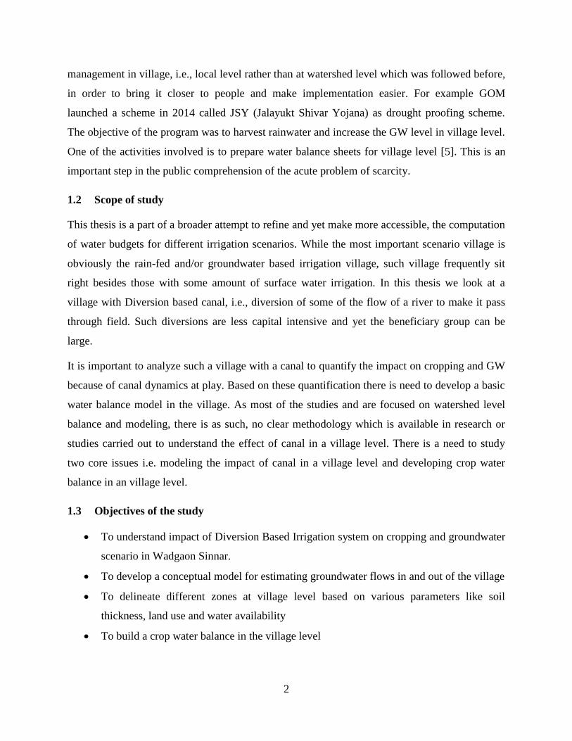
2.2.6 Initial zoning
Based on the initial study and past year scenario the village was zoned according to the region of
impact of canal, river and the stream as shown below (figure 2.11). Zoning was done to simplify
the understanding of village for analysis. Initial zone contained three zones namely R-C zone
(green) one between river and canal, C-S zone (light green) area between canal and the Dubere
stream and S-S zone (red) area after Dubere stream. Reason behind this being that R-C zone will
have good water scenario as river and canal contributed to its water resources. C-S zone will get
its contribution from hill side and S-S zone was critical zone as it was tanker fed part of the
village last year.
19
Figure 2.11: Initial zoning of village
Current zoning adopted in ground water modelling is explained in chapter 5.

20
3. Field level observation and analysis
Groundwater hydrology is an interpretive science; because we cannot observe the resource
directly, we must interpolate and extrapolate our understanding from known points of data and
observations. Also understanding these natural systems requires field level observation to record
its behaviour as observed in real time. Hence this chapter explains the observation recorded in
the Wadagon Sinnar village conducted through field visits over the duration of eight months.
3.1 Observation wells
Water-level measurements from observation wells are the principal source of information about
the hydrologic stresses acting on aquifers and how these stresses affect groundwater recharge,
storage, and discharge. Ideally the well chosen will provide data representation of various
parameter like water level, topographic condition, land use condition etc. In the study area as
most of the crop water requirement for the Rabi cropping is met by groundwater it becomes
imperative to understand the dynamics of the same in the area. Additionally the aquifer in the
region is unconfined as mentioned before. Hence the main purpose of the observation wells is to
survey and monitor the changes in groundwater aquifer studied for required time period.
3.1.1 Well network
A well network is a set of wells which are regularly measured. In a watershed the wells are
sampled based on various methods like random sampling, contour sampling where wells are
considered along a contour, cluster sampling etc. In the study area the sampling method adopted
to monitor 48 wells was transect sampling where in the wells where considered along four
different transect lines across the village. Transect method was adopted because of the presence
of the canal in the village. As seen in figure 3.1 there are four transects with each transect having
an average of 10 wells each. Wells were chosen in such manner that they are present on either
side of canal, river and within the village boundary. All the observation wells were located in the
farms, most of these wells served both the purpose of providing crop and drinking water
requirement. In this way the effect of canal, river on the groundwater can be monitored by the
routine well measurements[19]. In study area very few bore wells are present as compared to
open dug wells but they are not considered in the study.

21
Table 3-1: Well attribute list
Well
no.
Depth
(m)
Soil
depth
(m)
HR
depth
(mbgl)
Well
dia
(m)
Elevation
(m)
Min
dist
from
river
(m)
Min
dist
from
canal
(m)
mbgl(1) mbgl(2) mbgl(3)
WM
1 11.8 7 9 6 703 81 693 5 5.2 6.4
WM
2 14.7 6 12 6.5 704 118 706 5.5 5.8 6
WM
3 15.8 7.5 12.3 6.5 705 149 601 5.5 5.7 7.5
WM
4 14 5.8 8 6.5 707 225 480 4.3 5 8.6
Source: Observation wells recording
Figure 3.1 Observation Wells
3.1.2 Readings and analysis
Frequency of well measurement is an important part of water table monitoring system. The
interval between well readings in the study area was taken as 20 days. A total of 8 readings were
recorded starting from the month of November 2016 till April 2017. During well measurement,
care was taken to consider the water table level (mbgl) from the visible wetness in the well wall

22
and not actual water level to compensate the pumping from the well if present. Following figure
gives the elevation profile of wells in transect zone 1.
Figure 3.2: Well location elevation profile
As seen before the topology of the region slopes towards the river from the hill side part of the
village. Slope near the hill side is above 5% while near the river topology flattens out with slope
less than 5%. Other three transect also follow the same trends in terms of topology. Water table
contour map was plotted using the well level data for the month of November as seen in figure
3.3.
Figure 3.3: Ground water contour map
680
690
700
710
720
730
740
W1 W2 W3 W4 W5 W6 W7 W8 W9 W10 W11 W13 W14
Elev
atio
n in
m
Wells

23
The contour map gives initial water table scenario in the village which follows the regional
topology with the flow of water being towards the river. Wells near the river has better water
availability as its water table is recharged by both the topological gradient flow and canal flow.
The following table gives the average change in water levels in the wells between canal and river
during canal flow and after it ceased to flow (reading was recorded with interval of 21 days).
Table 3-2: Water table change in canal command and non command area
Average drop in water level well (m)
Command Area
During canal flow 0.5
After canal flow ceased 1.9
Non Command Area During canal flow 1.9
After canal flow ceased 2.5
Source: Field survey
Some of the physical observation based on the data obtained was
• In the areas where the soil thickness was more than 10m the drop per reading was on
average 1m.
• Soil thickness and slope had a direct correlation with water level in the well. As the wells
located in the hill side of the village had soil depth in the range if 1-3m which is less than
average thickness of soil in rest of the region and most of the wells had gone dry by the
month of January.
• There was transfer of water by pumping from the wells present near the canal and river to
the wells farm wells in hill side of the village.
• Water table/water availability on the Dubere side of the village was directly influenced
by filling of check dams built on the Dubere streams only.
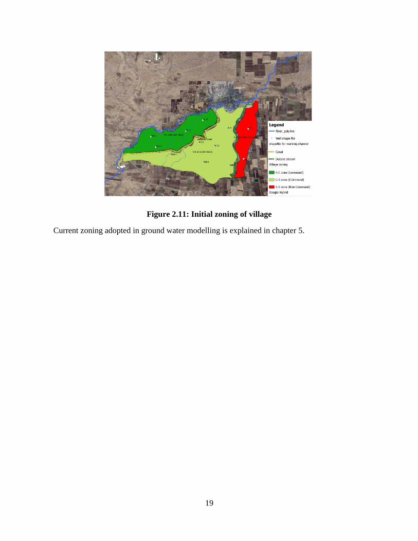
The following table gives the recharge rates observed in some wells in different months. This
was done by taking the reading of well after the pumping stopped followed by next reading after
a period of few hours.
24
Table 3-3: Well recharge rates
Sl no. Month First reading
(mbgl)
Second reading
(mbgl)
Recovery
(m)
Time (hr)
1 November 5.2 4.5 .6 1
2 January 8 7 1 13
3 March 14.3 14 0.3 6
4 April* 20.5 19.9 0.5 5
Well recharge rate for month of April was taken in the Dubere region (figure 2.2). In the
complete village this was the only region which had some farmers going for summer crops. Main
source of water for this part of village was through a stream called Dubere stream and it had a
significant impact on the wells in area. Interestingly this area was tanker fed area in summer of
2016 when the rainfall previous year was low. Many farmers mentioned that their wells got filled
to brim current year after a gap of 5 years. Finally the issues faced while recording these
observation wells were
• Inter well pumping- Here water is pumped into the wells from other wells which are
located near stream, river. This effects recording of wells as the water level is not the true
water level of the area. Prominent reason of pumping being that most of these wells are
located in hill zone (figure 2.2) where the water flows off too quickly due to low soil
thickness. One farmer in this area had a farm pond of 20m*20m*6m dimensions with a
of volume which took one month to fill with 2 pumps of 5hp capacity, when water is
available during the month of November he fills the farm pond so that Rabi crop water is
taken care off. Other reason being unbalance due to excessive cropping.
• Funny wells- these type of wells are very few but they always contradict the general
pattern of other wells in the area. It may be because of cracks present in murum
layer/hard rock, a natural water inflow path/spring etc.
3.2 Cropping data
Data on crops is an important aspect of analyzing the effect of groundwater dynamics in the
region. It helps in a getting a broader view of water stress/load in various part of the area. Hence
it is required to develop methodology to collect data of crops and its associated parameters.

25
3.2.1 Field survey
Survey was carried out in the Wadgaon Sinnar during the end of rabi season to record the
cropping patters in the village. It was seen to that most of the farm plots selected for survey was
the same plots where the observation wells were located. In this manner there could be a sort of
balance between the well reading and crop water requirement. There are three cropping seasons
namely
• Kharif season (June to September)
• Rabbi season (October to January)
• Summer season (February to May)
In study area 30 farms were surveyed asking various information like crops grown in various
season, number of watering per crop etc. Survey form is given in appendix A, most of the
surveyed plots had cropping for both Kharif and Rabbi seasons. Following graphs represents the
various observations recorded. The location of surveyed farms is given in figure 3.4.
Table 3-4: Cropping pattern of Major crops
Season Crops Cropping
percent
No. of
watering
(on average)
Type of irrigation Source
Kharif Soya bean 60 2 Rainfall/flood Canal/well
Other
vegetable
40 - Flood Well/canal
Rabi Wheat 38 8 Flood Well
Onion 41 7 Flood Well
Others 22 5-8 Drip/flood Well
Survey sample is 25 farmers with an total area of 32ha
Rabi season sees mostly the cropping of Onion and Wheat in the area. Other than wheat and
onion, crops like harbhara, garlic, potato etc are also grown. The dominant method of irrigating
the crops is flooding. It was noticed that the source of water for Rabi crops provided directly
through DBI system was negligible. Other observation was the regulation of flow into the canal
as the farms near the mouth of the canal had water logging condition. Around 2% of the area is

26
under horticulture which is mainly pomegranate. As horticulture requires water throughout the
year with the peak being during the period from flowering to harvesting (Jan-June) and next
harvest season (Sep to Jan), pomegranate farmers have bore wells and drip irrigation is used with
return flow fed back to the well. In the case of Kharif the major crop is soya bean followed by
corn, carrot, cauliflower etc, watering for these crops is through rainfall and flood irrigation
which depends on rain pattern. Summer cropping is sporadic in nature, but in the current year
2016-17 pockets of lands near Dubere stream had summer cropping because of good rainfall.
Crops usually grown during summer is Ground nut, Bajiri, cattle feed (grass) etc.
The cropping trend has not changed significantly over past few years, but there are few farmers
who have started cultivating sugarcane. Areas at the foothills of hill zone (figure 2.4) which
traditionally didn’t have cropping because of thin soil layer and lack of water availability during
Rabi season has seen cropping current year. The reason for this change is the availability of
water through wells located in canal command zone, stream and good rainfall. Figure 3.4 shows
the surveyed farm plots along with some plot taken from APS report of Gopal, some sugarcane
fields near to canal and cropping intensity. Its color coded to show the cropping season for farm.
Figure 3.4: Seasons of cropping for farm lands and survey location

27
3.2.2 LULC
Land use land cover (LULC) using remote sensing data gives a complete profile from bird point
of view of the study area in terms of cropping area, water resources and habitation in an area
with reasonable accuracy. LULC helps in mapping the modification in the cropping area over the
period of years. It is documented that there is significant impact on LULC change on a larger
agricultural watershed [20]. Datasets used for LULC is the USGS Landsat-8 and Sentinel
satellites imagery. Resolution of landsat-8 is 30m*30m while that of Sentinel 2 varies from
10m*10m in visible band to 60m*60m. One of the major limitations of these dataset is coarser
spatial resolution and inability to clearly distinguish between various crops. Also Landsat-8
images cannot be used for classification during monsoon season because of cloud cover over the
area.
Following figure gives the comparison between the LULC classification from Landsat-8 for the
Rabi (December) for the current year 2016-17 and previous year 2015-2016. Semi-automatic
QGIS plugin was used for classification. During classification, NDVI values were used with the
range of +1.0 to -1.0. Main classification in study area was of three type i.e. Crops, bare soil and
water bodies. As per literature, the Crops have a NDVI range of 0.6 to 0.9, shrubs and grass
lands have a range 0.2 to 0.3 while soils have a range of 0.1 to 0.2 [21]. Figure below depicts two
types of classification namely cropping and other being mixture of soil and sparsely spread
shrubs/grassland.
Figure 3.5: LULC for December 2015 and 2016

28
Comparing the LULC classification result of two consecutive years i.e. December 2015 and
December 2016 there is an increase in cropping area by 16%. This clearly indicates the effect of
good rainfall on the cropping area in the study area. The table below gives area of cropping and
soil area in the study region.
Table 3-5: LULC of study area
LULC Cropping area (ha) Cropping percent (of
geographical area)
Cropping percent (of
cultivable area)
December 2015 300 38% 43%
December 2016 425 54% 61%
Source: LULC classification
3.2.3 Secondary cropping data (TAO) and LULC
Every Taluka maintains the cropping data in its administrative area for both Kharif, Rabi and
summer season. Data shown below was collected from Taluk agricultural officer (TAO) in
Sinnar Taluk for the study area.
Table 3-6: Cropping report and LULC comparison
Village Area (ha) Cultivable land
(ha)
Rabi total
(ha) Cropping percent
Wadgaon
Sinnar
815 693
Rabi
TAO 160 23%
LULC 425 61%
Kharif TAO 562 81%
Source: TAO data 2016-17 and LULC classification Dec 2016

29
It can be seen from the table that there is difference in cropping percent for Rabi as calculated by
LULC and cropping report. A difference of 38% between LULC and cropping report is
observed. According to cropping report only 23% of cultivable land is cropped in study area
even though there was good rainfall during monsoon 2016. Table 11 shows the cropping area of
major crops as a percent of total cropped area in Rabi season comparing it with the data obtained
during the field survey (Table 8).
Table 3-7: Cropping report and field survey data
Data source Rabi crops Cropping area (ha) Cropping percent
Cropping report Wheat 70 10%
Onion 35 5%
Field survey Wheat 12 38%
Onion 14 41%
Source: TAO cropping data 2016-17 and field survey
There is lot of discrepancy in terms of cropping data recorded by agricultural office and the
sample data obtained by survey. Cropping report plays an important role in planning of water
management or development in the region. Usually the method adopted for collecting these data
is through agriculture assistant who visits village conducts surveys or collects data from the
Talathi. Basically they form the primary source of data collection. In these scenarios there are
chances of discrepancy in data as shown in the above table (which is of significant margin).
Hence it becomes imperative of TAO/administration to develop secondary methods of cropping
data verification like LULC mapping which can keep a check on data discrepancy. Adopting
such steps will tremendously improve the reliability and consistency of data obtained on
cropping.
3.3 Well loads
This section tries to calculate the water required on average per well for the cropping happening
in its vicinity. One of the assumptions considered is that most of the pumping happens during the
Rabi season. As for the Kharif season crops, major source of water is through rainfall and soil
moisture.
30
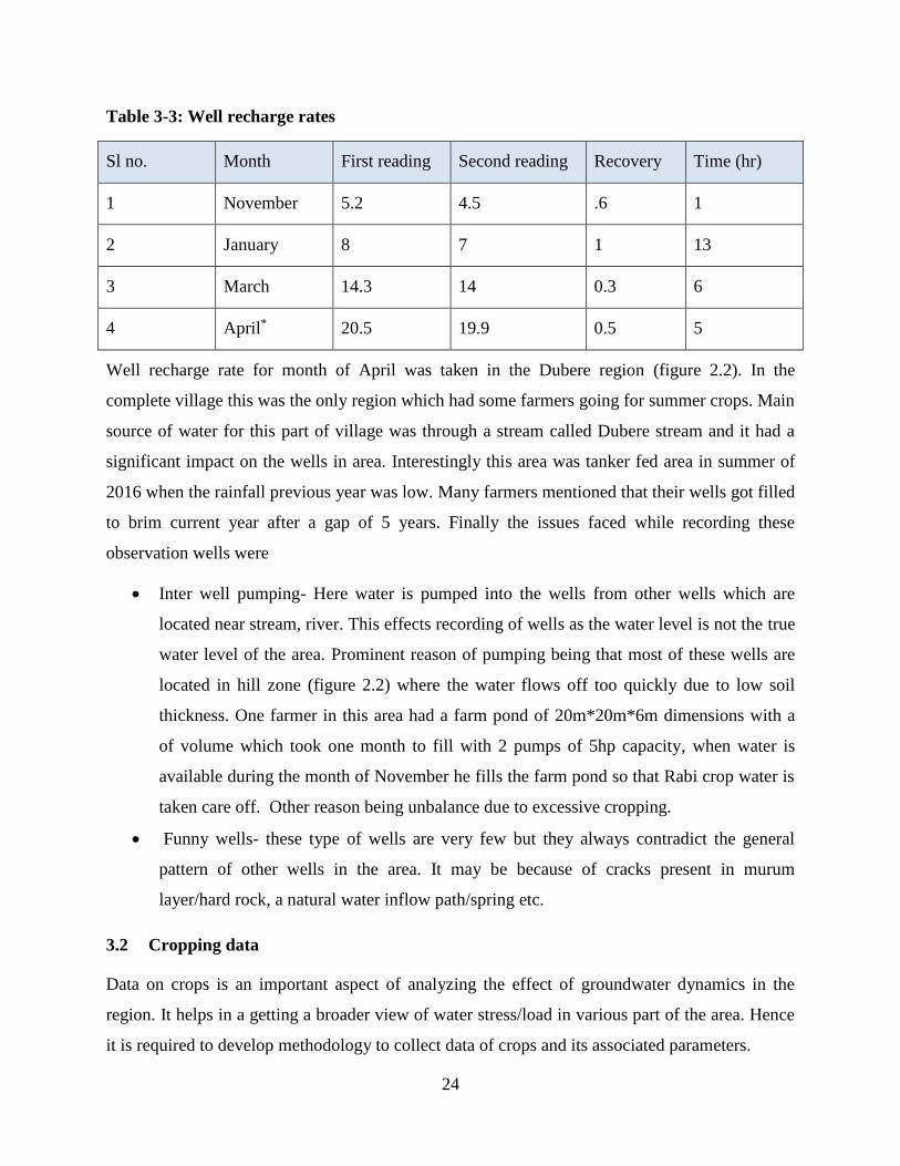
3.3.1 Cropping load
Taking the field survey data to consideration average area under each well comes around 1.5ha.
Wheat and onion are the main crops during Rabi season with around 80% cropping area.
Considering the ET load from the table below
Table 3-8: Crop water requirement
Sr.
No
Crop Sowing
time
Duration
(days)
Transition zone-I Scarcity zone
Water
need (mm)
Irrigation
need (mm)
Water
need (mm)
Irrigation
need (mm)
1 Soybean July 105 350-400 100-150 350-400 100-150
2 Bajari July 90 250-300 0-100 300-325 50-100
3 Groundnut July 120 450-500 200-250
4 Wheat Nov. 12 500-550 500-550 500-525 400-500
5 Harbhara Nov. 105 300-450 300-450 300-425 350-400
6 Grapes June - 1700-1800 1000-1200
7 Pomegranate July - 1200-1500 900-1000
10 Sugarcane Jan. 365 2000-2100 1600-1700 2000-2200 1600-1700
Source: WALMI crop water requirement booklets for farmers
By assuming 50% of cropping per farm as onion and rest of it wheat, table below computes an
average crop water requirement for a farm over a season
Table 3-9: Water requirement per farm
Water requirement for Wheat 3750m3/ 0.75ha
Water requirement for Onion 3000m3/ 0.75 ha
Total water requirement 6750m3/ 1.5 ha
31
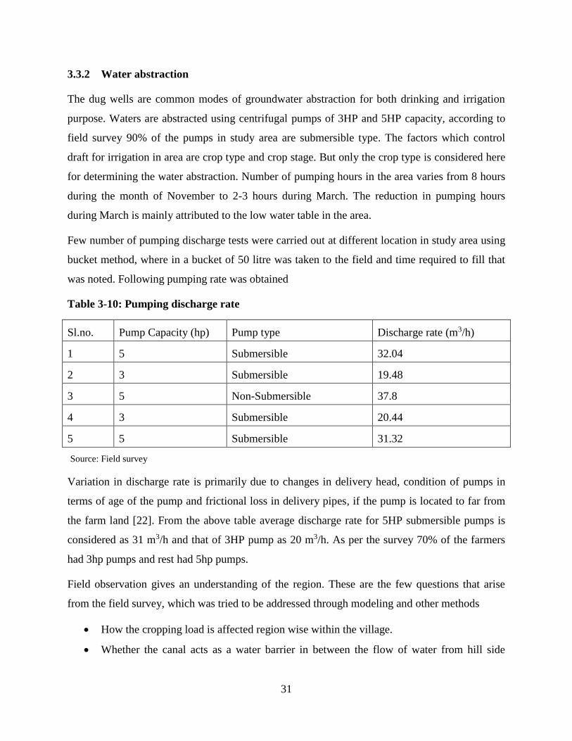
3.3.2 Water abstraction
The dug wells are common modes of groundwater abstraction for both drinking and irrigation
purpose. Waters are abstracted using centrifugal pumps of 3HP and 5HP capacity, according to
field survey 90% of the pumps in study area are submersible type. The factors which control
draft for irrigation in area are crop type and crop stage. But only the crop type is considered here
for determining the water abstraction. Number of pumping hours in the area varies from 8 hours
during the month of November to 2-3 hours during March. The reduction in pumping hours
during March is mainly attributed to the low water table in the area.
Few number of pumping discharge tests were carried out at different location in study area using
bucket method, where in a bucket of 50 litre was taken to the field and time required to fill that
was noted. Following pumping rate was obtained
Table 3-10: Pumping discharge rate
Sl.no. Pump Capacity (hp) Pump type Discharge rate (m3/h)
1 5 Submersible 32.04
2 3 Submersible 19.48
3 5 Non-Submersible 37.8
4 3 Submersible 20.44
5 5 Submersible 31.32
Source: Field survey
Variation in discharge rate is primarily due to changes in delivery head, condition of pumps in
terms of age of the pump and frictional loss in delivery pipes, if the pump is located to far from
the farm land [22]. From the above table average discharge rate for 5HP submersible pumps is
considered as 31 m3/h and that of 3HP pump as 20 m3/h. As per the survey 70% of the farmers
had 3hp pumps and rest had 5hp pumps.
Field observation gives an understanding of the region. These are the few questions that arise
from the field survey, which was tried to be addressed through modeling and other methods
• How the cropping load is affected region wise within the village.
• Whether the canal acts as a water barrier in between the flow of water from hill side

32
towards the river.
• Does the canal water account for change in cropping intensity in the area.
• What amount of water enters the village boundary through upper regions supplementing
the canal water for irrigation of crops.
• How the inter village groundwater flow happens

33
4. Introduction to basics of Groundwater Modelling
4.1 Need for technical analysis and Modelling
As seen in previous chapter the cropping water requirement in Wadagon Sinnar is largely
dependent on the situation of groundwater in the village. The flow in the canal ceases by the
month of November while the Rabi cropping of predominantly wheat and Rabi onion start during
this month with a cropping duration ranging from three to four months. During this period the
watering to the crops which is usually flood irrigation is provided by the wells in the farm. Hence
it is imperative to understand the groundwater dynamics in the village, this can be done by
building a groundwater model of the village. It also helps in understanding the flow of water into
the village and the canal’s region of impact within the village. Effects of future scenarios like
less rainfall and other parameters on the groundwater can be analyzed.
Finally as the DBI systems are being revived in the region there is a need to have technical
analysis to understand the current scenario in the village and impact of DBI system. So that it can
be replicated in other villages.
4.2 Science of Groundwater flow
In this section, the basic groundwater flow equation will be derived, which forms the basis for
groundwater modelling.
Some basic terms and terminologies:
Hydraulic head:
- The height of a column of water above datum is called hydraulic head or simply head or total
head. In the study of groundwater, head is the elevation of water in a well, where mean sea
level is used as a datum. Groundwater always flows in the direction of decreasing total head.
It has got three components.
a) Pressure head – It is measured from the bottom of the well to the top of the water level in
the well
b) Elevation head – It is measured from the mean sea level to the bottom of the well.
c) Velocity head – It represents the energy of a liquid due to its bulk motion, and is
generally neglected in groundwater flow study as is negligible.
34
Groundwater flow zones:
While studying groundwater flow, the subsurface is divided into three zones as follows:
- Unsaturated or vadose zone: It is the upper zone, just below the earth’s surface. Water in this
zone is dominated by the forces of adhesion and cohesion. It contains water held by the soils
and roots of the plants, and is also the link between water infiltrating in the ground and moving
down to the saturated zone. The pressure of water in unsaturated zone is less than atmospheric.
- Capillary fringe: This area is actually contained in both, the unsaturated and the saturated
zones, but the water in this zone is under the influence of surface tension i.e. it is the water
which has risen from the saturated ground water region due to capillary action. The pressure
here too is less than atmospheric pressure.
- Saturated or phreatic zone: Groundwater in this zone is fully saturated and is gravity driven.
The water here is at pressure more than atmospheric pressure. Water table is the imaginary
surface dividing unsaturated and capillary zones from saturated zone, at which the pore water
pressure is equal to atmospheric pressure. Below water table, all the pores of soil or rock are
fully saturated and pressure increases with depth.
Porosity:
It is the measure of the void or empty spaces in a material, and is a fraction of the volume of
voids over the total volume of the material and its value is between 0 and 1, or is expressed as
percentage. More the porosity of soil or rock, more easy is the water movement and storage
Hydraulic Conductivity:
It is the property of the plants, rocks or soils which describes the ease with which water can
move through pore spaces or fractures, which depends on the intrinsic permeability of the
material and on the degree of saturation expressed in [ L/T]
Heterogeneity and Anisotropy:
If the hydraulic conductivity K is independent of position within a geologic formation, the
formation is homogeneous. If K is dependent on position within a geologic formation, which is

35
always the case in groundwater systems, the formation is heterogeneous. In a homogeneous
formation, K(x, y, z) = C, C being constant; whereas in heterogeneous formation, K(x, y, z) ≠ C
If the hydraulic conductivity K is independent of the direction of measurement at a point in a
geologic formation, the formation is isotropic at that point. If the hydraulic Conductivity K
varies with the direction of measurement at a point in a geologic formation, the formation is
anisotropic at that point. If an x, y, z coordinate system is set up in such a way that the
coordinate directions coincide with the principal directions of anisotropy, the K values in the
principal directions can be specified as Kx, Ky, Kz. At any point ( x, y, z ), an isotropic formation
will have Kx=Ky=Kz, whereas an anisotropic formation will have Kx≠Ky≠Kz.
Specific storage:
It is the amount of water that a portion of an aquifer releases from storage, per unit volume of
aquifer, per unit change in hydraulic head while remaining fully saturated.
Specific yield:
It is the quantity of water, unit volume of an aquifer will yield by gravity, when fully saturated
and expressed as a ratio or as a percentage of the volume of the aquifer.
Continuity equation of groundwater flow:
Consider the flow of ground water taking place within a small cube (of lengths ∆x, ∆y and ∆z
respectively the direction of the three areas) in a saturated zone where 𝜌 is the density of water
and 𝑉𝑥 , 𝑉𝑦, 𝑉𝑧 are the velocity components of water in x, y and z directions.
Figure 4.1:Continuity equation for ground water flow

36
The total incoming water in the cubical volume should be equal to that going out. Thus,
defining inflows and outflows as
Inflows:
In x-direction: 𝝆𝒗𝒙(∆𝒚. ∆𝒛)
In y-direction: 𝝆𝒗𝒚(∆𝒙. ∆𝒛)
In z-direction: 𝝆𝒗𝒛(∆𝒙. ∆𝒚)
Outflows:
In X-direction: 𝝆 (𝒗𝒙 +𝝏𝒗𝒙
𝒗𝒙∆𝒙) (∆𝒚. ∆𝒛)
In Y-direction: 𝝆 (𝒗𝒚 +𝝏𝒗𝒚
𝒗𝒚∆𝒚) (∆𝒙. ∆𝒚)
In Z-direction: 𝝆 (𝒗𝒛 +𝝏𝒗𝒛
𝒗𝒛∆𝒛) (∆𝒙. ∆𝒚)
The net mass flow per unit time through the cube is,
[𝝏𝒗𝒙
𝒗𝒙+
𝝏𝒗𝒚
𝒗𝒚+
𝝏𝒗𝒛
𝒗𝒛] (∆𝒙. ∆𝒚. ∆𝒛)
According to conservation principle sum of these three quantities should be zero, thus
𝝏𝒗𝒙
𝒗𝒙+
𝝏𝒗𝒚
𝒗𝒚+
𝝏𝒗𝒛
𝒗𝒛= 𝟎 − − − − − (𝟒. 𝟏)
The above equation is the equation of continuity in groundwater flow.
4.2.1 Darcy’s Law
The water flow just observed during the derivation of continuity equation is due to the
difference in hydraulic head per unit length in the direction of flow. Henry Darcy, a French
engineer was the first to suggest and derive a relation between the velocity as seen in the
continuity equation and the hydraulic gradient.

37
Figure 4.2: Darcy's law
According to his experiments, the discharge Q passing through a tube of cross-sectional area A
filled with a porous material is directly proportional to the difference of hydraulic head h
between the two end points and inversely proportional to the flow length L.
Thus, 𝑸 ∝ 𝑨 .𝒉𝟏− 𝒉𝟐
𝑳
He introduced the proportionality constant K i.e. hydraulic conductivity of the porous material,
which finally makes the equation as
𝑸 = −𝑲𝑨𝒅𝒉
𝒅𝑳− − − − − (𝟒. 𝟐)
Where,
-Negative sign is introduced because the hydraulic head decreases in the direction of flow.
-𝑑ℎ
𝑑𝑙 is the hydraulic gradient
4.3 Basic differential equation of groundwater flow
Substituting Darcy’s Law in the equation of continuity we get,
𝝏
𝝏𝒙(𝑲𝒙
𝝏𝒉
𝝏𝒙) +
𝝏
𝝏𝒚(𝑲𝒚
𝝏𝒉
𝝏𝒚) +
𝝏
𝝏𝒛(𝑲𝒛
𝝏𝒉
𝝏𝒛) = 𝟎 − − − − − (𝟒. 𝟑)
Here, hydraulic conductivities in the three directions are assumed to be different i.e. for
anisotropic medium. If isotropic medium with constant hydraulic conductivity in all directions is
considered, the equation becomes,
𝑲 (𝝏𝟐𝒉
𝝏𝒙𝟐+
𝝏𝟐𝒉
𝝏𝒚𝟐+
𝝏𝟐𝒉
𝝏𝒛𝟐) − 𝑾𝒔 = 𝟎 − − − − − (𝟒. 𝟒)
38
This equation, also known as Laplace’s equation (appears in many places in mathematical
physics) is known as the basic equation governing the groundwater flow. The basic problem in all
the groundwater models is to find the solution to this Laplace’s equation.
As the conservation principle has been applied for deriving this equation, it means that no mass is
gained or lost or there is no net inward flux or outward flux to or from this system. Thus, this
equation is for the steady incompressible groundwater flow where heads don’t change with time.
Now, if the heads change with time, the conservation principle cannot be applied. Hence, some
mass will be gained or lost with time depending upon the heads. So there will be change in
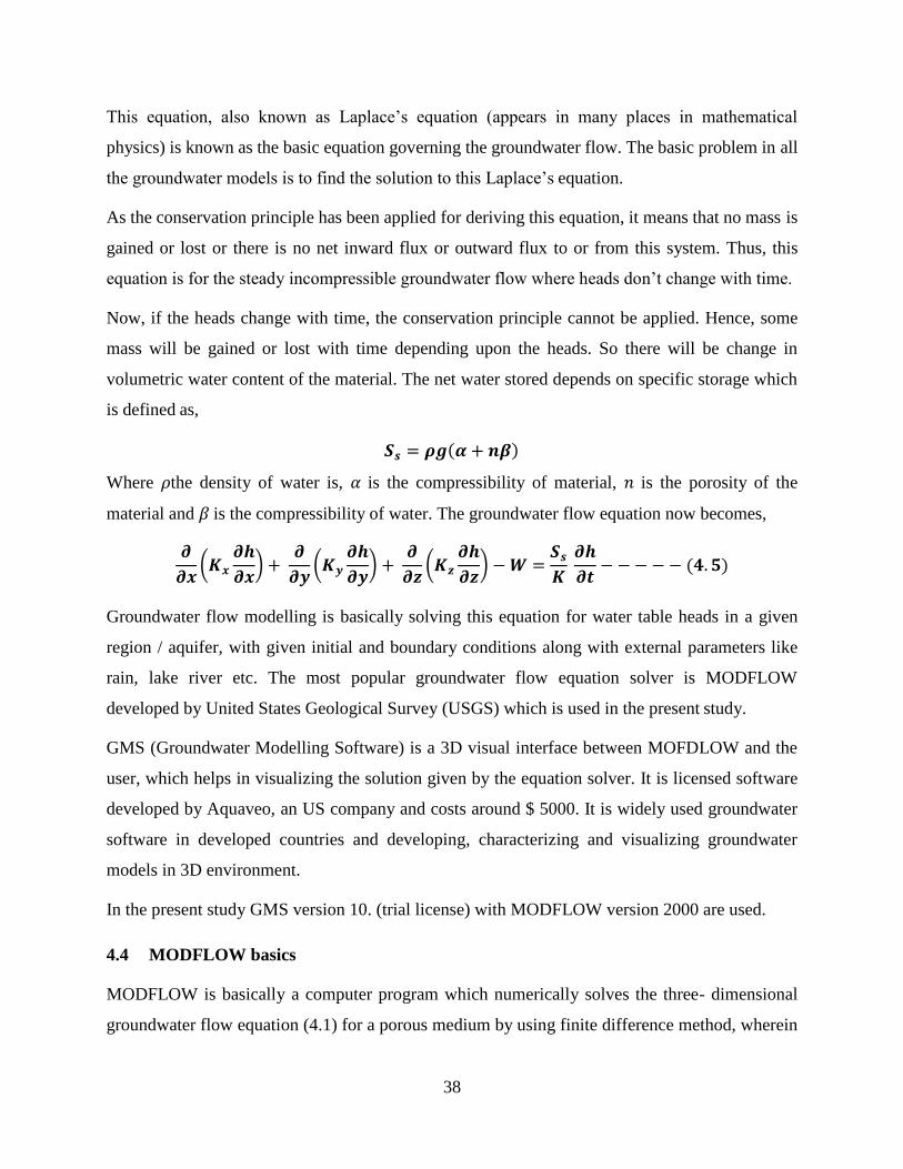
volumetric water content of the material. The net water stored depends on specific storage which
is defined as,
𝑺𝒔 = 𝝆𝒈(𝜶 + 𝒏𝜷)
Where 𝜌the density of water is, 𝛼 is the compressibility of material, 𝑛 is the porosity of the
material and 𝛽 is the compressibility of water. The groundwater flow equation now becomes,
𝝏
𝝏𝒙(𝑲𝒙
𝝏𝒉
𝝏𝒙) +
𝝏
𝝏𝒚(𝑲𝒚
𝝏𝒉
𝝏𝒚) +
𝝏
𝝏𝒛(𝑲𝒛
𝝏𝒉
𝝏𝒛) − 𝑾 =
𝑺𝒔
𝑲 𝝏𝒉
𝝏𝒕− − − − − (𝟒. 𝟓)
Groundwater flow modelling is basically solving this equation for water table heads in a given
region / aquifer, with given initial and boundary conditions along with external parameters like
rain, lake river etc. The most popular groundwater flow equation solver is MODFLOW
developed by United States Geological Survey (USGS) which is used in the present study.
GMS (Groundwater Modelling Software) is a 3D visual interface between MOFDLOW and the
user, which helps in visualizing the solution given by the equation solver. It is licensed software
developed by Aquaveo, an US company and costs around $ 5000. It is widely used groundwater
software in developed countries and developing, characterizing and visualizing groundwater
models in 3D environment.
In the present study GMS version 10. (trial license) with MODFLOW version 2000 are used.
4.4 MODFLOW basics
MODFLOW is basically a computer program which numerically solves the three- dimensional
groundwater flow equation (4.1) for a porous medium by using finite difference method, wherein

39
the continuous system described the equation (1) broken down into finite set of discrete points in
space and time, and the partial derivatives are replaced by terms calculated from the differences
in head values at these points. This process leads to systems of linear algebraic difference
equations whose solution yields values of head at specific points and times. The values obtained
are approximates to the time-varying head distribution. that would have been given by analytical
solution of the partial differential equation of flow [23]
The MODFLOW uses finite difference equation to solve the problem. This is done by applying
the above continuity equation to the model which is the sum of all flows into and out of cell must
be equal to the rate of change in storage within the cell. At the heart of MODFLOW lies spatial
discretization of an aquifer system with a mesh of blocks called cells, the locations of which are
described by rows, columns and layers.
Figure 4.3:MODFLOW grid
The finite difference equation which forms the basis of MODFLOW, is derived by applying the
continuity equation seen above i.e. the sum of all flows into and out of the cell must be equal to
the rate of change in storage within the cell. Thus, assuming density of water as constant again,
the continuity equation for the balance of flow in a cell will be

40
1
2
∑ 𝑸𝒊 = 𝑺𝒔
∆𝒉
∆𝒕∆𝑽
Where,
𝑄𝑖 is the flow rate into the cell
𝑆𝑠 is the specific storage; volume of water which can be injected per unit volume of aquifer
material per unit of change in head
∆𝑉 is the volume of the cell and
∆ℎ is the change in head over a time interval ∆𝑡
For the simulation to start, two types of inputs are necessary:
Initial head distribution – The initial head distribution provides a value of ℎ𝑖,𝑗,𝑘at each point in the
mesh i.e. it provides the values of head at the beginning of the first of the discrete time steps
into which time axis is divided in finite-difference process. The first step is to find solution
for ℎ𝑖,,which marks the end of first step and so on.
Boundary conditions – The groundwater flow equation is solved by solving the boundary
value problem. Boundary value problem is a differential equation with additional constraints,
called boundary conditions. In MODFLOW, the boundary conditions can be set at the
beginning, by entering the status of certain cells in the mesh in advance. There are three kinds
of boundary conditions:
- Known head or constant head – the head for some cells is specified in advance, and this
head remains constant throughout the simulation
- Known flow – the flow into or out of particular cell is known beforehand.
- No flow – These are the cells for which the flow into or out of the cell is permitted, in
any time step in the simulation.
4.4.1 Iterative methods
Each time step in the simulation in MODFLOW starts by arbitrarily assigning a trial value or
estimate for the head at each cell at the end of that step. A procedure for calculation is then started
which alters these estimated values, producing a new set of head values which are in closer
agreement with the system of equations. These new, or interim, head values then take the place of
the initially assumed heads, and the procedure of calculation is repeated, producing a third set of

41
head values. This procedure is repeated successively, at each stage producing a new set of
interim heads which more nearly satisfies the system of equations. Each repetition of the
calculation is termed as iteration. Finally the changes made by the succeeding stages become
very small, and this smallness is utilized in determining when to stop the iteration also termed as
closure criterion or convergence criterion.
Thus, during a MODFLOW simulation, series of iterations form one time step, series of time
steps form one stress period and user can enter multiple stress periods each with specific stress
data like monsoon period data, post-monsoon period data etc. [24]
4.4.2 Packages
The modular structure of MODFLOW consists of a Main program and a series of highly
independent sub-routines called modules. The modules are in turn grouped into packages. Each
package deals with the specific feature of hydrologic system which is to be simulated, such as
simulation of a well, simulation of a lake, simulation of an underground barrier structure,
simulation of stream, simulation of drains, rains etc. [24]
The packages used in the current modeling are
LPF: Layer property flow package, this package is used to define flow properties in the model.
The parameters which are part of package and for which inputs are to be defined in array format
are horizontal/vertical conductivity (HK/VK) for each layer. One can also enter horizontal
anisotropy values on a cell by cell basis.
Drain: The Drain package is used to simulate the effect of drains on an aquifer. Drains remove
water from the aquifer as long as the water table is above the elevation of the drain. If the water
table falls below the elevation of the drain, the drain has no effect. The rate of removal is
proportional to the difference in elevation between the water table and the drain. The constant of
proportionality is the conductance of the fill material surrounding the drain. Other package is
DRT package where in the removed water can be reintroduced to the aquifer at a specified grid
cell.
Recharge: The Recharge package is used to simulate recharge to an aquifer due to rainfall and
infiltration. Recharge is typically defined by specifying a recharge value for each cell for each
vertical column in the grid. The recharge value represents the amount of water that goes into the

42
groundwater system and not the amount of precipitation. The units of recharge are length/time. It
can also be used in simulating evapotranspiration (ET) as the EVT package used for
evapotranspiration in the MODFLOW is not able to successfully depict the ground condition.
Here a negative value is given for recharge depicting the removal of water from the cell.

43
5. MODFLOW for Wadgaon Sinnar Area
To build a model lot of input parameters are required. Many of these parameters have already
been calculated like the watershed boundary, catchment area, DEM of the region, streams, rivers
etc. In addition to these there are some parameters which are vital for building of the model both
conceptual and actual but have to be derived from the existing data set collected from field
observations and surveys. This chapter lays out the process involved from deriving such a
parameter to the MODFLOW simulation of the model. Initial section talks about the steps
followed to get boundary head estimation equation using well readings which was used to define
the boundary condition in the model. This part is followed by the section which explains the
conceptual model of the study area which is paramount for modeling. Following which
groundwater model is built and simulated in MODFLOW based on the conceptual model. The
simulation and its resulting analysis are described in the third section of the chapter. Final section
of this chapter is reserved for conclusion and future works. In brief four sections are
• Boundary head estimation equation
• Conceptual Model
• Model building and analysis
• Conclusion
As the village is part of a larger watershed, modeling requires defining of a boundary condition
of the village. Determining boundary condition is important as it will determine the water inflow
and outflow from the study area. In case the simulation involves complete watershed, then
usually boundary conditions are considered as no flow regions because they lie along the ridge
lines[25]. But this is not the case with respect to study area as it is a part of a watershed and it is
pertinent to determine the boundary head values of the village. Following section will discuss
about developing this boundary condition using numerical model.
5.1 Boundary head estimation equation
GW table in study area is an unconfined aquifer and the head at any point is equal to elevation of
the water table above the base of aquifer. An unconfined aquifer is bounded at the bottom by
material that is considered impermeable. In chapter 4.1 there were 48 observation wells with 8
readings recorded. Basically in an aquifer the water table mimics the topology of the region.

44
Also the wells recording showed similar reading. There was a total of 384 data points, it was
decided to develop linear regression model on these data set.
Water table is influenced by multiple parameters which have to be quantified and its impact on
water table level to be determined. So a well point in the study area is dependent basically on
two factors i.e. spatial and temporal. In case of spatial factor a well is affected by it location i.e.
latitude and longitude and its elevation above MSL as shown in figure below
Figure 5.1: Topology of a well
The temporal factor is the change in water level in the well over interval of time. Other factors
which were incorporated initially were minimum distance of well from the river, minimum
distance of well from the canal, slopes between well, distance from contour lines. All these factor
were parameterized and multiple linear regressions method was used. Initial linear equation was
as follows
𝑊 = 𝑎𝑋 + 𝑏𝑌 + 𝑐𝑍 + 𝑑𝑅 + 𝑒𝐶 + 𝑑𝑇 + 𝑒𝑇𝑍 + 𝐾 − − − −(5.1)
In above equation
W is the water level in well
X is the longitude
Y is the latitude
Z is the elevation

45
R is the minimum distance from the river to the well
C is the minimum distance from the canal to the well
T is the time interval
K is the equation constant
Minimum distance algorithm was used to calculate the minimum distance to river and canal in
QGIS. The various values thus obtained are shown in the snap shot of excel below
Figure 5.2: Initial linear equation condition
Lat and long are of different units hence the current coordinate system is projected into pseudo
Mercator 3857-WGS 54 system where the units are in meter/distance projection. Now all the
parameters are in same unit and distance co-ordinate system. The problem faced at this stage was
the enormity in the value of the data which led to scale issues while computing coefficients of
linear regression equation a, b, c, d etc using matrix method. To overcome this error the well
point with least latitude (𝑌𝑚𝑖𝑛), least longitude (𝑋𝑚𝑖𝑛) and least geographical elevation (𝑍𝑚𝑖𝑛) in
the study area was deducted from all the well points. Hence the values were rescaled through
following changes.
𝑋𝑟𝑒−𝑠𝑐𝑎𝑙𝑒𝑑 = 𝑋𝑎𝑛𝑦−𝑝𝑜𝑖𝑛𝑡 − 𝑋𝑚𝑖𝑛 − − − − − (5.2)
𝑌𝑟𝑒−𝑠𝑐𝑎𝑙𝑒𝑑 = 𝑌𝑎𝑛𝑦−𝑝𝑜𝑖𝑛𝑡 − 𝑌𝑚𝑖𝑛 − − − − − (5.3)
𝑍𝑟𝑒−𝑠𝑐𝑎𝑙𝑒𝑑 = 𝑍𝑎𝑛𝑦−𝑝𝑜𝑖𝑛𝑡 − 𝑍𝑚𝑖𝑛 − − − − − (5.4)
Re-scaled values X and Y were then divide by 100 and following sheet was obtained

46
Figure 5.3: Re-scaled values
Once the values were set, outliers from well data were removed and 40 wells were chosen for
analysis. Time of initial well reading was taken as t=0 and final reading as t=135 with the
intervals of t=21, 42 etc corresponding to different well recordings (each time step had dataset of
40 well readings).
Linear regression for different parameter combinations were tried out and its R2 determined.
Table below represents R2 for some of those combinations
Table 5-1: R-squared values
Combinations R2 value
X, Y, Z, R, C, T, TZ 0.35
X, Y, Z, C, T, TZ 0.43
X, Y, Z 0.38
X, Y, Z, T 0.61
X, Z, T 0.69
Source: Calculated values
It can be seen that the combination X, Z, T had the best R2 value, hence it was selected as water
table predicting equation. Now eqn.4 reduces to
𝑊 = 𝑎𝑋 + 𝑐𝑍 + 𝑑𝑇 + 𝐾 − − − − − (5.5)
The co-efficient obtained for above equation is as follows,
a= 0.0429; c= 0.1353; T=0.0754 and K= -1.1739
Now for any point in the study area and a given time a predicted well value can be determined by
above equation.

47
5.2 Conceptual model
To solve an natural system or site specific problem, one must assemble and analyze relevant field
data and articulate important aspects of GW system. The synthesis of what is known about the
site is called conceptual model [26].
5.2.1 Methodology of building the conceptual model
To understand groundwater flow into a system/village it is important to understand boundary
condition defining the village/system. So for better analysis of village, the boundaries of the
village were defined on basis of topology and field observation in the village.
Groundwater flows: In the study area in-flow of groundwater after monsoon is from surface
flows (canal) and subsurface flows. The Village is located in the plateau after the Sahyadri hill
ranges and GW flows into the village from the south side boundary and joins the river as seen in
figure 5.4.
Figure 5.4: Boundary Condition

48
The contributor to these flows entering from the southern part of study area is the hill ranges
present at a distance of 6km from the village. Factors which influence this subsurface flow are
rainfall in the region, ET load from cropping in villages present between the study area and hill
range, water conservation structures etc.
Now to know the amount of groundwater entering the village through southern boundary,
groundwater heads (water table level) along the boundary has to be found. This can be found by
two methods. First method is to develop groundwater model for the complete watershed of
which the village is part off and then demarcate southern village boundary in the model to know
the groundwater heads along the boundary. This method was not feasible due to the lack of data
on the watershed level to build the groundwater model. Other method developed to determine
the groundwater heads along the boundary was based on well readings recorded in the study
area. Using eight well readings recorded over a period of six months a linear regression equation
was built (Equation 8) which was based on three factors namely location of well, elevation of
well and time period. The Linear regression equation was used to determine the heads along the
southern boundary of the village.
Heads obtained along the boundary was considered as constant heads i.e. groundwater heads
which remain constant for a given period of time, providing groundwater flows into the village.
Canal and river flow: Northern side of the village boundary borders along the river as shown in
the figure above. As there is flow in the river the heads along the river are considered constant
head with the heads being equal to the elevation of the river bed. Similarly the case with canal
when it is operational, the canal provides a constant head along its length i.e. through constant
seepage to groundwater. The region between the canal and river is influenced because of this
constant head seepage from the canal. On the other hand the presence of constant groundwater
head creates a water head lump as shown in the figure below (the figure shown below is obtained
after simulating the model in MODFLOW, which will be explained in section 5.3). As a result of
this lump, water flowing from upper region is ‘walled’ and more water is available to the upper
region. In other words canal (DBI) not only provides water to the command area between canal
and river but it also helps in improving water availability in the upper regions of the area to a
certain extent.

49
Figure 5.5: Cross section of canal
Figure 5.6: Lump effect
(Source: MODDFLOW)
Watershed Boundary: Here Eastern boundary of the village is along the watershed boundary of
the region and hence it’s considered as no flow boundary (figure 2.9). So there three boundaries
defined for the study area i.e. GW flow boundary in southern part of the area, river constant head
boundary on the northern part and no flow boundary on eastern side. All these boundaries will
help in determining the flow in the study area.

50
Steady state and Transient state: In steady state condition hydraulic head doesn’t change with
time i.e. the amount of water that flows into the system, is the same as that flows out of the
system equation 2 (chapter 4) . Transient condition is a case where hydraulic head varies with
time which is given by equation 3 (chapter 4). In a complete watershed when all the boundary
condition is considered no flow which means the boundary condition remains constant over the
period of time.
Considering modeling transient condition in the study area required continuous change in the
boundary condition of the study area i.e. boundary condition changes over the period of time.
Simulating which became complex due to lack of data. Hence in the current study a steady state
is considered which capture an instant of transient state condition on a typical DBI operational
day.
5.3 Modeling and analysis
5.3.1 Initial Condition
In many GW models, hydrological parameter estimation often remains the most difficult
problem that many studies try to overcome by assigning uniform values or by dividing the
parameters values into classes corresponding to different part of the area which can be adjusted
by calibration [27]. Modeling was based on distributed parameter model which helps in
representing more realistic distribution of system properties.
Conceptual model was built in MODFLOW using 9 coverages for the study area. Coverage
defined properties like hydraulic conductivity, ET load zones, budget zones, specific head etc.
Thickness of aquifer was divided into two layers. The boundary of the village was drawn
according to the administrative boundary. There are two drains/stream in the villages which were
mapped and the conductance was kept initially as at 25 m2/day/m. Dubere stream which had
check dams were modeled defining check dam regions as constant heads. The initial range for
conductivity of the top layer as per literature was considered in the range of 1 to 3 m/d, while
hydraulic conductivity of the lower layer had the range of 0.5-0.89m/d [28]. Vertical
conductivity was considered half of horizontal conductivity. Different recharge zones were
demarcated and mapped. Wells and drainage coverage was set based on the observation well
data and QGIS derived data.

51
Figure 5.7: MODFLOW Conceptual model
3-d grid model
A Grid was generated by taking a cell size of 30m*30m, elevations of the grid was taken from
DEM and mapped to the top layer of the grid. Thickness of first layer varied from 15m to 20m
and second layer had the constant thickness of 10m. For boundary condition the specified heads
at river and canal was defined as top layer elevation while the specified head at hill side was
defined using eqn.8. as explained in conceptual model.
Figure 5.8: 3-d grid model
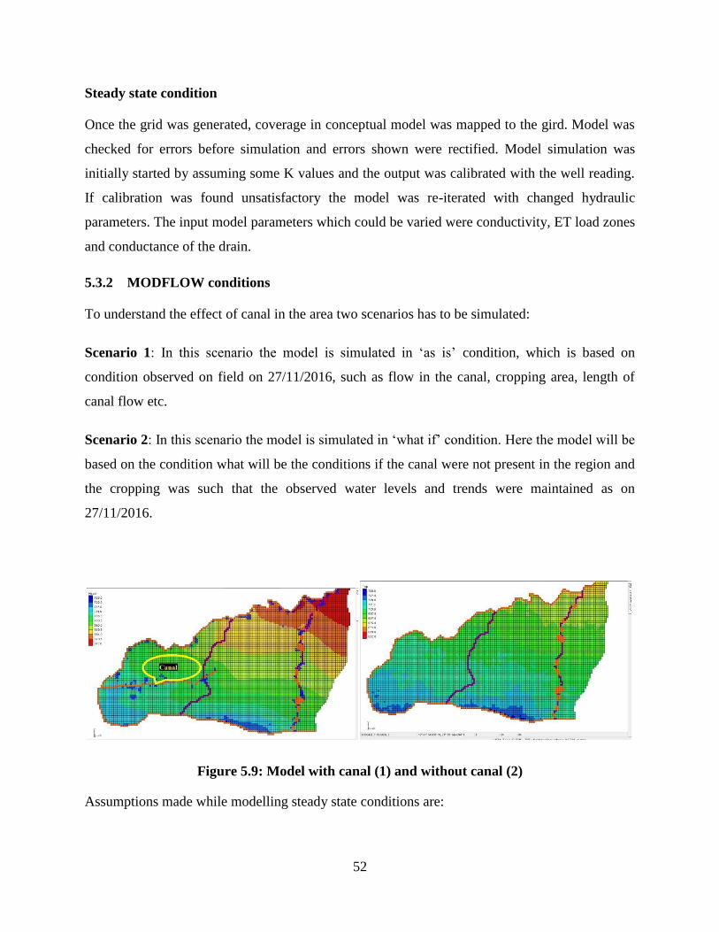
52
Steady state condition
Once the grid was generated, coverage in conceptual model was mapped to the gird. Model was
checked for errors before simulation and errors shown were rectified. Model simulation was
initially started by assuming some K values and the output was calibrated with the well reading.
If calibration was found unsatisfactory the model was re-iterated with changed hydraulic
parameters. The input model parameters which could be varied were conductivity, ET load zones
and conductance of the drain.
5.3.2 MODFLOW conditions
To understand the effect of canal in the area two scenarios has to be simulated:
Scenario 1: In this scenario the model is simulated in ‘as is’ condition, which is based on
condition observed on field on 27/11/2016, such as flow in the canal, cropping area, length of
canal flow etc.
Scenario 2: In this scenario the model is simulated in ‘what if’ condition. Here the model will be
based on the condition what will be the conditions if the canal were not present in the region and
the cropping was such that the observed water levels and trends were maintained as on
27/11/2016.
Figure 5.9: Model with canal (1) and without canal (2)
Assumptions made while modelling steady state conditions are:

53
• Cropping pattern in the area is categorized into Onion, Wheat and Others. The ET load
for same is considered as 400mm, 500mm and 350mm.
• Cropping ratio for Onion, Wheat and Others is divided into 35%, 35% and 30%
respectively.
• Similarly cropping duration is considered as 120 days for Onion and Wheat and 90 days
for other crops. (Based on the field survey)
• Sowing for Rabi crops started after the festival of Deepawali in month of October.
The ET load is obtained from the literature for each crop. Study area is divided into ET zones as
shown in figure. Zones were determined based on factors like land use, canal flow region,
topology etc.
Figure 5.10: ET zones
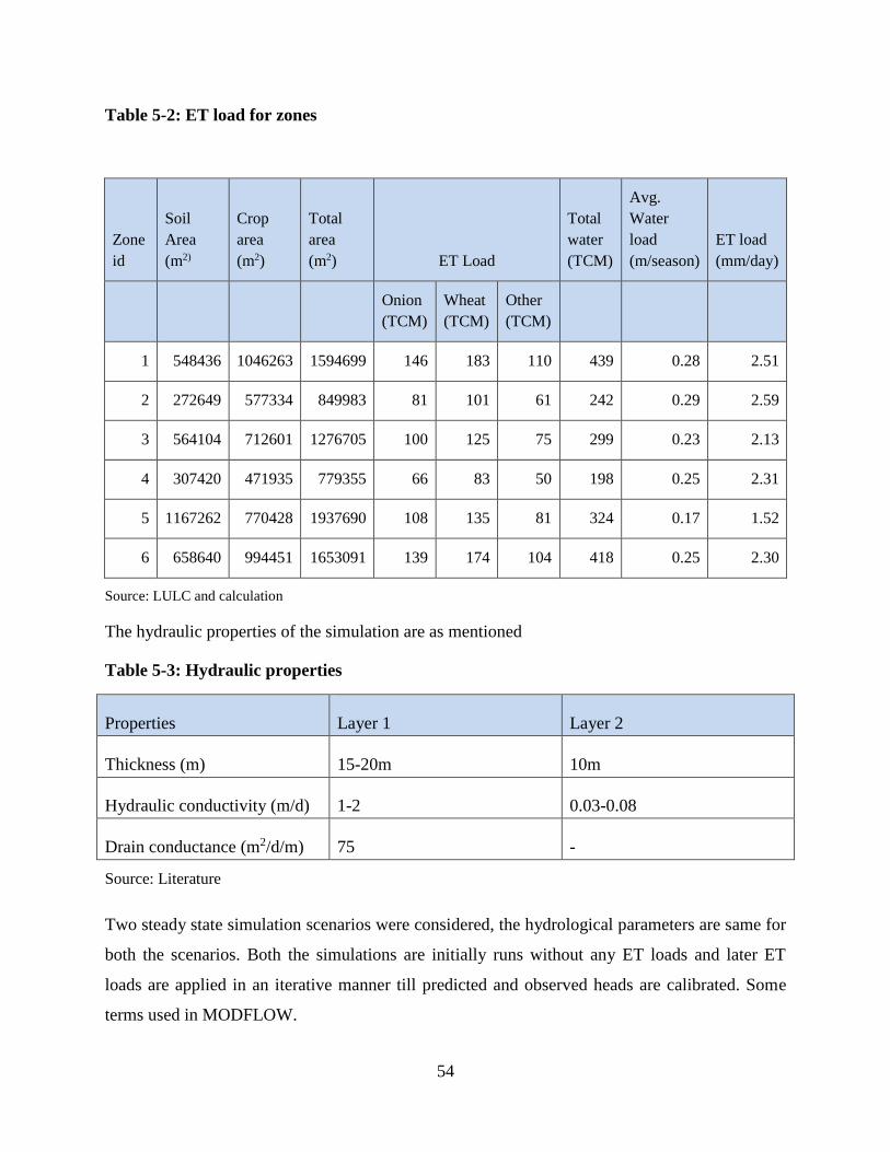
54
Table 5-2: ET load for zones
Zone
id
Soil
Area
(m2)
Crop
area
(m2)
Total
area
(m2) ET Load
Total
water
(TCM)
Avg.
Water
load
(m/season)
ET load
(mm/day)
Onion
(TCM)
Wheat
(TCM)
Other
(TCM)
1 548436 1046263 1594699 146 183 110 439 0.28 2.51
2 272649 577334 849983 81 101 61 242 0.29 2.59
3 564104 712601 1276705 100 125 75 299 0.23 2.13
4 307420 471935 779355 66 83 50 198 0.25 2.31
5 1167262 770428 1937690 108 135 81 324 0.17 1.52
6 658640 994451 1653091 139 174 104 418 0.25 2.30
Source: LULC and calculation
The hydraulic properties of the simulation are as mentioned
Table 5-3: Hydraulic properties
Properties Layer 1 Layer 2
Thickness (m) 15-20m 10m
Hydraulic conductivity (m/d) 1-2 0.03-0.08
Drain conductance (m2/d/m) 75 -
Source: Literature
Two steady state simulation scenarios were considered, the hydrological parameters are same for
both the scenarios. Both the simulations are initially runs without any ET loads and later ET
loads are applied in an iterative manner till predicted and observed heads are calibrated. Some
terms used in MODFLOW.

55
MODFLOW ET load: ET load applied in the MODFLOW model.
Actual ET load: ET truly acting in the area/zones calculated by LULC mapping.
Calculated drop: The drop in the water table in a given period of time due to applying
MODFLOW ET load instead of actual ET load.
Obs. Drop: Drops observed in the field recorded by well level reading.
So drop from MODFLOW ET load is calculated by
𝑊𝑆 = 𝑊𝑡 − 𝑆𝑦
∆ℎ
∆𝑡− − − − − (5.6)
Where M_ET is the ET applied in MODFLOW model
ET is the actual ET calculated
Sy is the specific yield considered as 2.5%
∆h is the change in the water table
∆t is the change in time considered as 21 days.
Scenario 1: In this scenario canal is active and flowing. The model is run for a condition nearly
mimicking the actual situation present in the village i.e. by considering the actual cropping in the
village, flows in the canal etc. and model is iterated till the predicted head matches the observed
head (well reading) in the study area. By simulating the model with above mentioned conditions
we get following output (Table 17).

56
Figure 5.11: Heads output
Figure 5.12: Calibration plot
To quantify the flow in the region, flow budget is computed by classifying various zones for
canal, hill, Dubere region. (Appendix B)
Table 5-4: Zone budget
All units in TCM/day ZONE 1 ZONE 2 ZONE 3 ZONE 4
Region Canal-River Canal Hill side Dubere area
IN IN IN IN

57
CONSTANT HEAD 1.57 2.94 3.52 1.81
FROM ZONE 1 0.00 0.05 0.00 0.09
FROM ZONE 2 1.02 0.00 0.23 0.12
FROM ZONE 3 0.00 0.40 0.00 0.90
FROM ZONE 4 0.09 0.15 0.41 0.00
Total IN 2.69 3.55 4.15 2.93
OUT OUT OUT OUT
CONSTANT HEAD 1.16 0.72 0.78 0.43
DRAINS 0.00 0.41 0.25 0.86
ET 1.38 1.03 1.82 0.97
TO ZONE 1 0.00 1.02 0.00 0.10
TO ZONE 2 0.06 0.00 0.40 0.02
TO ZONE 3 0.00 0.23 0.00 0.41
TO ZONE 4 0.09 0.13 0.90 0.00
Total OUT 2.70 3.50 4.16 2.93
Source: MODFLOW
Total flow in and out of the system is 9.856 TCM. From the table, water entering from hill side is
3.52 TCM of which most of the water is lost because of ET loads and rest is either entering zone
4 or leaving system by constant head. Zone 2 with canal has an inflow of 2.94 TCM from
constant head and with inflow from Zone 3 restricted to areas where canal being inactive.
Outflow in Zone 2 is 1.03 TCM and 0.72 TCM by constant head. Effective water entering
because of canal is 2.24 TCM.
Recalling the values form table 4, water percolation rate in the canal is 24lps amounting to 2.07
TCM /day which is nearly same as that of modelled value. Now Zone 1 gets 1.03TCM of water

58
from canal area which explains the better cropping intensity in this zone 1(65% of Zone 1
geographical area is cropped).
Table 5-5: ET loads comparison
ET zones
MODFLOW ET
load (mm)
Actual
ET (mm)
Difference
(mm)
Calculated
drop for 21
days (m) Obs. Drop (m)
Zone 1 1.3 2.51 1.21 1.01 0.4
Zone 2 1 2.59 1.59 1.34 2.3
Zone 3 0.8 2.13 1.32 1.2 1.8
Zone 4 0 2.31 2.31 1.94 1.3
Zone 5 0.3 1.52 1.22 1.02 1.2
Zone 6 0.6 2.30 1.70 1.43 1.6
Comparing the true ET loads acting on the zones and MODFLOW ET load applied to calibrate
the wells on these zones, drop in water table over period of 21 days is calculated using equation
9. Later calculated drop is compared with actual drop recorded. The difference in drops between
calculated and observed values for various regions are in the range of 0.1 to 0.9, this may be
attributed to well reading and model parameter errors.
Scenario 2: Here to simulate the model without canal it is assumed that farmers change the
cropping area to observe the same calibration well levels as that of scenario 1. This will give the
amount of cropping area reduction required to observe the same well level as scenario 1, in other
words to determine the amount of cropping area which will give similar well levels as the one
recorded with presence of functional canal but with no canal flow .
Then the model is simulated under same condition as that of scenario 1. MODFLOW ET loads
are iterated to match calibration value of that scenario 1.

59
Figure 5.13: Output heads
Figure 5.14: Calibration plot for Scenario 2
Zone budget for this scenario is given in the following page.

60
Table 5-6: Flow budget for Scenario 2
All units in TCM/day ZONE 1 ZONE 2 ZONE 3
IN IN IN
Regions River side Hill Side Dubere side
CONSTANT HEAD 1.92 3.82 1.74
FROM ZONE 1 0.00 0.19 0.24
FROM ZONE 2 1.00 0.00 0.48
FROM ZONE 3 0.28 0.13 0.00
Total IN 3.20 4.15 2.40
OUT OUT OUT
CONSTANT HEAD 1.68 1.02 0.58
DRAINS 0.22 0.12 0.53
ET 0.85 1.51 0.96
TO ZONE 1 0.00 1.00 0.29
TO ZONE 2 0.19 0.00 0.13
TO ZONE 3 0.24 0.48 0.00
Total OUT 3.20 4.15 2.48
Source: MODFLOW
In the flow budget without canal, most of the GW flows are from the hill side. Off the 2.8 TCM
water from Zone 2, 1 TCM enters the zone 1. This shows that the zone 1 will have better GW
availability even in the absence of canal when compared with other zones but not enough to
sustain old cropping pattern i.e. cropping pattern with canal.

61
Table 5-7: ET load comparison of scenario 1 and scenario 2
ET zones
MODFLOW ET
load (mm)
Scenario 1
MODFLOW ET
load (mm)
Scenario 2
Actual ET
(mm)
Difference
in ET loads
(mm)
New
actual ET
load
(mm)
Zone 1 1.3 0.3 2.51 1 1.47
Zone 2 1 0.3 2.59 0.7 1.89
Zone 3 0.8 0.8 2.13 0 2.13
Zone 4 0 0 2.31 0 2.31
Zone 5 0.3 0.3 1.52 0 1.52
Zone 6 0.6 0.6 2.30 0 2.30
Source: MODFLOW and calculation
5.3.3 Analysis
From table 5.7 it can be seen that there is drop in MODFLOW ET load in the zones 1 and 2 of
magnitude 1 and 0.7 mm while other zones are not affected when the canal is not active. In other
words it means that without the canal ET load has to drop by 1 and 0.7mm in zones 1 and 2 to
sustain the observed well level. Also the canal command area which is between the canal and
river (zone 1) is obviously affected by the absence of canal. Interesting aspect is the effect of
canal on zone 2 which is not a part of command area as it is upstream/ upper region of the canal.
It is seen that in the absence of the canal, this zone is affected adversely. This clearly indicates
the ‘blocking’ of groundwater flows from the upper regions by the canal resulting creation of
‘water banks’ for the upper regions.

62
Figure 5.15: Zones of canal influence
The influence of canal on the upper region of the study area is shown through the cross section
view of the GW table in the figures below
Figure 5.16: Water table with and without canal
In simulation between flow and no flow scenarios of canal the change in actual ET load observed
are 1.51 and 1.89mm. The corresponding change in cropping area in the zone 1 and zone 2 are
given in the table below.

63
Table 5-8: Cropping area with and without canal
Scenarios Area (ha)
Cropping area
(ha) Cropping percent
ET load
(mm)
Zone1 With Canal 160 104 65 2.5
Without canal 160 63 39 1.5
Zone2 With Canal 85 58 68 2.59
Without canal 85 44 51 1.89
Note: Zone 4 is also influenced by the canal as the canal extends up to the end of zone 4 but the
scenario for which the MODFLOW model was simulated, canal was active only till end of zone
1. Hence the canal influenced could not be captured on zone 4.
The ground water stock variation in the study area over the period of time obtained from the well
readings is shown in the graph below
Figure 5.17:Variation of groundwater stock over the period of time
The drop in the GW stock is linear till the month of March and after that the drop becomes more
gradual as the GW stock is kept for drinking water security and protective irrigation.
0
500
1000
1500
2000
2500
3000
3500
Sto
ck in
TC
M
Time period
GW-Stock
GW-Stock (TCM)

64
Finding:
• The percentage decrease in cropping area in zone 1 without canal is 39%
• Percentage decrease in cropping area in zone 2 without canal is 24%
• Overall decrease in the total cropping area of 425ha without canal is 14%
• Amount of water added by canal to the system is 2.24 TCM/day.

65
6. Conclusion
• The benefit of canal (DBI) is substantial as the impact of canal is not restricted to the
command area but also to the non command area. As the canal ‘blocks’ the flow of water
from the upstream side /hill side there by providing water to the non command area.
• Zone budget shows that the amount of water entering from hill side during canal flow is
5.27 TCM/day and without canals its 2.8 TCM/day. Hence presence of canal increases
water flow in the hill side.
• The cropping pattern in directly dependent on canal water in the canal influence zones.
While zones like Dubere area and areas near the base of the hill are outside the ambit of
Canal Zone of influence.
• The change in total cropping area due to absence of canal is 14% while that in command
area is 40% and uphill region (zone 2) is 24%.
• Cost of infrastructure per hectare for rejuvenation of a DBI system is approximately
Rs.55000/ha.
• Rejuvenation of DBI is an feasible option and better than conventional canal irrigation
system.
6.1 Scope for future works
• To run the transient condition model of the village by developing the complete watershed
groundwater model to determine the changing boundary flows.
• Understandings inter-well water transfer acting in the area and transfer of water from one
zone to another.

66
7. References
[1] S. Asia and G. Forum, “Water and Agriculture in India Background paper for the South
Asia expert panel during the Global Forum for Food and Agriculture,” p. 3, 2017.
[2] N. Planning Commission (India), “Report of the expert group on ground water
management and ownership,” New Delhi Gov. India, no. September, pp. 1–70, 2007.
[3] N. Planning Commission (India), “Water management and irrigation,” Plan. Comm.,
2012.
[4] P. D. Udmale, Y. Ichikawa, A. S. Kiem, and S. N. Panda, “Drought Impacts and
Adaptation Strategies for Agriculture and Rural Livelihood in the Maharashtra State of
India,” Open Agric. J., vol. 8, no. 1, pp. 41–47, 2014.
[5] G. Resolution and N. C.- Case, “Water for all -Drought-free Maharashtra 2019 Regarding
implementation of Jalyukta Shivar Campaign to permanently overcome internal drought
situation. Government of Maharashtra,” 2014.
[6] P. K. Srivastava and R. M. Singh, “Groundwater assessment in a canal command area for
sustainable irrigation in a part of the Indo-Gangetic alluvial plain,” Curr. Sci., vol. 112,
no. 3, pp. 478–489, 2017.
[7] C. A. Sullivan, J. R. Meigh, and A. M. Giacomello, “The Water Poverty Index:
Development and application at the community scale,” Nat. Resour. Forum, vol. 27, no. 3,
pp. 189–199, 2003.
[8] A. A. Sokolov, “The Unesco Press Paris 1974,” 1974.
[9] H.-Y. Sun, C.-M. Liu, X.-Y. Zhang, Y.-J. Shen, and Y.-Q. Zhang, “Effects of irrigation on
water balance, yield and WUE of winter wheat in the North China Plain,” Agric. Water
Manag., vol. 85, no. 1–2, pp. 211–218, 2006.
[10] G. P. Kruseman and De Ridder, N.A., “Analysis and evaluation of pumping test data,” Int.
Inst. L. Reclam. Improv. Wageningen, Netherlands. Publ. 47, 1970.
[11] V. Srinivasan, “Reimagining the past - Use of counterfactual trajectories in socio-
hydrological modelling: The case of Chennai, India,” Hydrol. Earth Syst. Sci., vol. 19, no.
2, pp. 785–801, 2015.
[12] D. Nasik, “Comprehensive District Agriculture Plan C-DAP 12 th Five Year Plan
Collector , Nasik District Superintending Agriculture
Officer , Nasik.”
[13] “Introduction to DBI.” [Online]. Available:
http://www.indiawaterportal.org/articles/ripple-tide-film-sdtt-its-work-local-ngos-and-
communities-diversion-based-irrigation.
[14] Aditya, “Working of DBI.” [Online]. Available:
http://adityabastola.blogspot.in/2007/06/phad-system.html.
[15] “Musalgaon census.pdf.” .
[16] GSDA Pune, “Report on the Dynamic Ground Water Resources of Maharashtra (2011-

67
2012),” no. March, p. 167, 2014.
[17] M. Of, W. Resources, C. Ground, W. Board, G. W. Information, and N. District, “Ground
water information Nashik District,” 2014.
[18] M. Dept. of Agriculture, “Agro climatic zones.” [Online]. Available:
http://www.mahaagri.gov.in/CropWeather/AgroClimaticZone.html.
[19] C. J. Taylor and W. M. Alley, “Ground-water-level monitoring and the importance of
long-term water-level data,” Geol. Surv. Circ., no. 1217, pp. 1–76, 2001.
[20] K. E. Schilling, M. K. Jha, Y.-K. Zhang, P. W. Gassman, and C. F. Wolter, “Impact of
land use and land cover change on the water balance of a large agricultural watershed:
Historical effects and future directions,” Water Resour. Res., vol. 44, no. 7, 2008.
[21] J. L. Hatfield and J. H. Prueger, “Value of using different vegetative indices to quantify
agricultural crop characteristics at different growth stages under varying management
practices,” Remote Sens., vol. 2, no. 2, pp. 562–578, 2010.
[22] D. Saha and A. K. Agrawal, “Determination of specific yield using a water balance
approach - Case study of Torla Odha watershed in the Deccan Trap province, Maharastra
State, India,” Hydrogeol. J., vol. 14, no. 4, pp. 625–635, 2006.
[23] B. A. W. Harbaugh, E. R. Banta, M. C. Hill, and M. G. Mcdonald, “MODFLOW-2000 ,
The U .S . Geological Survey modular graound-water model — User guide to
modularization concepts and the ground-water flow process,” U.S. Geol. Surv., p. 130,
2000.
[24] Aquaveo LLC, “GMS User Manual ( v8 . 3 ) The Groundwater Modeling System,” 2012.
[25] M. Anderson, W. W. Woessner, and R. Hunt, Applied Groundwater Modeling, Second
Edition: Simulation of Flow and Advective Transport. 2015.
[26] N. K. A. Mikszewski, Hydrogeological Concpetual Site Models. .
[27] H. El Idrysy and F. De Smedt, “Modelling groundwater flow of the Trifa aquifer,
Morocco,” Hydrogeol. J., vol. 14, no. 7, pp. 1265–1276, 2006.
[28] Ministry of Water Resources, “Report of the Ground Water Resource Estimation
Committee: Ground Water Resource Estimation Methodology,” p. 113, 2009.

68
Appendix A: Farmer survey questionnaire

69
Appendix B: Water budget zones