jump process for the trend estimation of time seriesplaza.ufl.edu/yiz21cn/refer/jump process for...
TRANSCRIPT
Computational Statistics & Data Analysis 42 (2003) 219–241www.elsevier.com/locate/csda
Jump process for the trend estimation oftime series
Shan Zhaoa , G.W. Weia;b;∗aDepartment of Computational Science, National University of Singapore, Singapore 117543, Singapore
bDepartment of Mathematics, Michigan State University, East Lansing, MI 48824, USA
Received 1 January 2001; received in revised form 1 March 2002; accepted 1 March 2002
Abstract
A jump process approach is proposed for the trend estimation of time series. The proposedjump process estimator can locally minimize two important features of a trend, the smoothnessand 0delity, and explicitly balance the fundamental tradeo2 between them. A weighted averageform of the jump process estimator is derived. The connection of the proposed approach to theHanning 0lter, Gaussian kernel regression, the heat equation and the Wiener process is discussed.It is found that the weight function of the jump process approaches the Gaussian kernel, as thesmoothing parameter increases. The proposed method is validated through numerical applicationsto both real data analysis and simulation study, and a comparison with the Henderson 0lter.c© 2002 Elsevier Science B.V. All rights reserved.
Keywords: Jump process; Time series; Trend estimation; Nonparametric regression; The smoothness-0delitytradeo2; Weighted average form; Gaussian kernel
1. Introduction
In the additive model of the time series, it is assumed that the economic time seriesis made up of three components, the trend, the cyclic (seasonal) component, and theirregular component (random noise),
yt = Tt + St + �t ; t = 1; 2; : : : ; N; (1)
where random variable yt is the observation at a discrete time t, Tt and St are trendand seasonal component, respectively, and N is the length of the time series. Here, �t
∗ Corresponding author.E-mail address: [email protected] (G.W. Wei).
0167-9473/02/$ - see front matter c© 2002 Elsevier Science B.V. All rights reserved.PII: S0167 -9473(02)00125 -1

220 S. Zhao, G.W. Wei / Computational Statistics & Data Analysis 42 (2003) 219–241
is random noise and is usually assumed to be stationary and of zero mean. From theviewpoint of mathematical modeling, trend is not a well-de0ned concept, see Kennyand Durbin (1982), Harvey (1989), Chat0eld (1996), Mosheiov and Raveh (1997),and Franses (1998). In general, trend may be considered as “long-term smooth changein the mean level”.
To carry out in-depth statistical study of time series, it is often necessary to converta nonstationary series into a stationary one before the statistical model is treated. Inother words, time series will be decomposed into individual trend, seasonal, and ir-regular components. Conventionally, there are two di2erent ways to decompose a timeseries which does not consist of seasonal component (or is seasonally adjusted): di2er-encing and detrending. The di2erencing will remove trend, while the detrending (trendestimation) will present an estimate to trend. Thus, the di2erencing and detrendingare essentially high-pass 0lter and low-pass 0lter, respectively, from the viewpoint ofdigital signal processing (DSP). It is noted that a debate has been arisen about theappropriate selection between these two alternative ways for economic and 0nancialtime series, and the issue remains unresolved, see Nelson and Plosser (1982), Sims(1988), Sims and Uhlig (1991), Campbell and Perron (1991), Cochrane (1991), andthe special issue of Vol. 6 (1991) of the Journal of Applied Econometrics.
Since the nonstationary trend component sometimes can be of more interest than thenoise, the trend estimation techniques have attracted a lot of research interests in theliterature, see for example, Kenny and Durbin (1982), Goodall (1990), Ball and Wood(1996), Mills and Crafts (1996), Mosheiov and Raveh (1997), Canova (1998), Blanchiet al. (1999), Wen and Zeng (1999), Ferreira et al. (2000), and Pollock (2000). In fact,the trend estimation is potentially useful for data interpretation, long-term forecastingand for the study of real business cycle. In some cases, the detection of trend is evena crucial task, see for example Visser and Molenaar (1995). Therefore, it is practicallyuseful to accurately estimate the trend component of time series.
Generally speaking, methods of trend estimation fall into two major categories: para-metric and nonparametric. In the parametric approach, a deterministic trend is com-monly expressed by a particular smoothing function or model, such as a polynomial,the Gompertz curve or the logistic curve (Meade and Islam, 1995), or the structuraltime series model (Harvey, 1989). However, the use of an inappropriate parametricmodel may cause misleading information and even incorrect inference about the trendcurve. Therefore, alternative nonparametric trend estimation methods are widely used.In particular, nonparametric approaches o2er considerable Lexibility in the selection of0tting curves and may yield satisfactory estimates. In conventional time series analysis,some of the most widely used nonparametric approaches include moving average 0ltersand exponential smoothing 0lter, which are linear low-pass 0lters in the sense of theDSP. A variety of moving average 0lters are proposed, such as Spencer 0lter (Kendallet al., 1983), Henderson 0lter (Kenny and Durbin, 1982), and GLAS 0lter (Blanchiet al., 1999), etc. The asymmetric exponential smoothing 0lter (Kenny and Durbin,1982) has a distinguished advantage in the treatment of boundary e2ect, hence is oftenpreferred for the purpose of forecasting.
Apart from these linear 0lters, various nonparametric regression estimators existingin the literature can be easily adopted for the purpose of trend estimation. This is
S. Zhao, G.W. Wei / Computational Statistics & Data Analysis 42 (2003) 219–241 221
because that the counterpart of trend component Tt in the content of nonparametricregression is just the regression function T (xt),
yt = T (xt) + �t ; t = 1; : : : ; N; (2)
where x and y are explanatory and response variable, respectively. Many powerfulnonparametric regression estimators have been proposed and applied in the literature,such as kernel smoothing (MNuller, 1988), LOESS (Cleveland, 1979), locally weightedpolynomial regression (Fan and Gijbels, 1996), smoothing spline (Eubank, 1999), andregression spline (Doksum and Koo, 2000). Furthermore, there are also many interest-ing studies suggested in the literature in order to enhance the performance of nonpara-metric regression estimators, such as improving the accuracy (e.g., Borra and Ciaccio,2002), dealing with special data (e.g., Keilegom et al., 2001), and so on. In fact, thenonparametric regression has been successfully used in trend estimation, see for ex-ample HNardle and Tuan (1986), Goodall (1990), Hart (1991, 1994), HHst (1999), andFerreira et al. (2000). Other nonparametric trend estimation methods that were studiedin the literature include: Hodrick Prescott (HP) 0lter (Hodrick and Prescott, 1997),median 0lter (Wen and Zeng, 1999), wavelet shrinkage (Donoho et al., 1995), andlinear programming (Mosheiov and Raveh, 1997). Usually, a successful nonparametricmethod has one or more underlying smoothing parameters which can be adjusted tobalance the fundamental tradeo2s of the estimates, i.e., the smoothness-0delity tradeo2and the variance-bias tradeo2.
What is more relevant to the present work is a class of nonparametric trend estimationmethods that attempt to globally quantify the competition between the two conLictingfeatures: the smoothness and the 0delity. The earliest motivation to this approach datesback to 1923 when Whittaker (1923) introduced graduation, which is also one of theearliest works of nonparametric regression in the literature. By using the residual sumof squares
∑Nt=1 (yt − Tt)2 as the global measure of 0delity of the estimated trend Tt ,
Whittaker (1923) suggested to de0ne the sum of the squares of kth order di2erencesas the measure of roughness. Then the optimal trend is given by solving the followingminimization scheme:
(WH): min{Tt}N
t=1
{N∑t=1
(yt − Tt)2 + �2N−k∑t=1
(�kTt)2
}; (3)
where order k and smoothing parameter � are user-speci0ed constants and � is thedi2erence operator.
A particular example following Whittaker’s approach is the HP 0lter (Hodrick andPrescott, 1997), which has been most extensively used in the real business cycle liter-ature for detrending
(HP): min{Tt}N
t=1
{N∑t=1
(yt − Tt)2 + �N∑t=1
(Tt−1 − 2Tt + Tt+1)2
}: (4)
Hodrick and Prescott recommended setting � = 1600 when applying to real businessstudies. By manipulating the relevant 0rst-order condition, the HP scheme leads to atwo-way moving average with weights subjected to a damped harmonic approximately,see King and Rebelo (1993).
222 S. Zhao, G.W. Wei / Computational Statistics & Data Analysis 42 (2003) 219–241
Recently, a popularly used measurement of the roughness penalty of estimates T (xt)in nonparametric regression is
∫[T ′′(x)]2 dx. This leads to following penalized least-
squares regression scheme:
(SS): min{Tt}N
t=1
{N∑t=1
(yt − Tt)2 + �∫
[T ′′(x)]2 dx
}; (5)
which is known as smoothing spline estimator. Remarkably, the problem of optimiza-tion SS over the space of all twice di2erentiable functions on the interval [a; b]=[x1; xN ]has a unique solution T�(x) which is de0ned as the natural cubic spline, see Eubank(1999) and references therein.
More recently, Mosheiov and Raveh (1997) (MR) proposed a linear programmingapproach to estimate the trend by employing the sum of the absolute values ratherthan the common sum of squares to measure the smoothness and 0delity. The tradeo2balancing leads to such an optimization scheme
(MR): min{Tt}N
t=1
{�
N∑t=1
|yt − Tt | + (1 − �)N−2∑t=1
|Tt+2 − 2Tt+1 + Tt |}
: (6)
Through a trick of variable changing, the objective function of the minimization schemeMR will be free of the absolute operator. However, extra constraints, monotonicity orpolytonicity, have to be forced upon estimates in order to uniquely solve the lin-ear programming problem. The location of the changing points of polytone trend iscase-dependent and its selection is somewhat arbitrary.
Obviously, all these optimization schemes are closely related. The pointwise rough-ness measure of MR, Tt+2−2Tt+1 +Tt , is essentially the same as those of HP and WH,and is the discrete version of SS. Instead of forward di2erence, Tt+2 − 2Tt+1 + Tt , thebackward and central di2erence approximation may also be used in the optimizationMR. Moreover, with appropriate boundary modi0cations (such as in HP 0lter, see Bax-ter and King, 1995), the summation of the global smoothness measure in WH and MRcan be processed from 1 to N , which may be more reasonable in a comparison withthe integration in SS. Apart from their common motivation, another common feature ofthis class of nonparametric approaches is their use of global implicit minimization. Asis well known, a global minimization problem can be quite expensive for its numericalcomputation.
The main objective of this paper is to present a new nonparametric approach, jumpprocess, to estimate the unknown deterministic trend function of a time series. In con-trast to the global implicit minimization approach, a localized approach is developedfor trend estimation. The proposed jump process can locally minimize both characteris-tics and explicitly balance the fundamental tradeo2 between them. A weighted averageform of the jump process estimate is derived in the present paper, so that the im-plementation of jump process becomes extremely simple. The connection between thepresent jump process approach and the traditional trend estimation methods, as well asthe DSP is discussed. It is found that the weight function of the jump process 0lterapproaches the normal kernel, as the smoothing parameter increases.
This paper is organized as follows. The formalism of the jump process is introducedin Section 2. Numerical techniques regarding di2erent implementations and boundary
S. Zhao, G.W. Wei / Computational Statistics & Data Analysis 42 (2003) 219–241 223
modi0cations are discussed in detail. The method is illustrated through applications toseveral real price series and one simulated example in Section 3. Conclusions are givenin Section 4.
2. Theory and algorithm
2.1. Local measurement of smoothness and 6delity
A common feature of optimization schemes WH, HP, SS and MR is to minimizethe linear combination of the global measure of 0delity and smoothness, while using a“smoothing parameter” to balance the tradeo2 between 0delity and smoothness. Thereare three key aspects in the design of these nonparametric trend estimation approaches:
(1) De0ne measures for 0delity and smoothness,(2) balance the tradeo2 by employing a smoothing parameter,(3) minimize the linear combination of two measures to achieve an estimate which is
optimal in the sense of the given measures.
In the present study, an iterative jump process will be considered, which actuallyadmits a simpler optimization approach for trend estimation
TM+1t = TM
t + R(TMt−1 − 2TM
t + TMt+1)
= TMt + R�2TM
t
T 0t = yt; t = 1; : : : ; N; (7)
where ratio R (R¿ 0) and iteration parameter M are user-speci0ed constants. Thesecond term on the right-hand side of iterative process (7), TM
t−1 − 2TMt + TM
t+1, is thepointwise measure of smoothness. To have a better understanding of this iterative jumpprocess, TM
t of Eq. (7) is rewritten in terms of yt :
TMt = yt + R
M−1∑k=0
�2Tkt ; t = 1; : : : ; N: (8)
Further denote vM−1t =
∑M−1k=0 �2Tk
t , this yields
(yt − TMt ) + RvM−1
t = 0; t = 1; : : : ; N: (9)
It is obvious that the 0rst term on the left-hand side of (9), (yt − TMt ), is the local
measure of the 0delity, while the second term, vM−1t , is the accumulative local measure
of smoothness. At each step of the iteration, this process guarantees that the sum of thelinear combination of the local deviation from yt and the accumulative local measureof smoothness equals to zero. In the sense of such local minimization, the optimalestimated trend is the output of iterative jump process (7) by using yt as input. Sucha trend estimation method will be referred as a jump process estimator.
In terms of minimization, the relationship between the jump process and the opti-mization schemes WH, HP, SS, and MR is somewhat analogous to the relationship
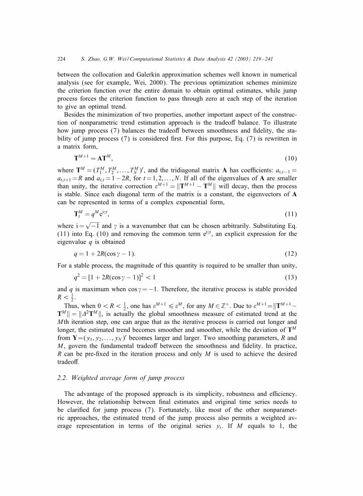
224 S. Zhao, G.W. Wei / Computational Statistics & Data Analysis 42 (2003) 219–241
between the collocation and Galerkin approximation schemes well known in numericalanalysis (see for example, Wei, 2000). The previous optimization schemes minimizethe criterion function over the entire domain to obtain optimal estimates, while jumpprocess forces the criterion function to pass through zero at each step of the iterationto give an optimal trend.
Besides the minimization of two properties, another important aspect of the construc-tion of nonparametric trend estimation approach is the tradeo2 balance. To illustratehow jump process (7) balances the tradeo2 between smoothness and 0delity, the sta-bility of jump process (7) is considered 0rst. For this purpose, Eq. (7) is rewritten ina matrix form,
TM+1 = ATM ; (10)
where TM = (TM1 ; TM
2 ; : : : ; TMN )′, and the tridiagonal matrix A has coeScients: at; t−1 =
at; t+1 =R and at; t =1−2R, for t =1; 2; : : : ; N . If all of the eigenvalues of A are smallerthan unity, the iterative correction �M+1 = ‖TM+1 − TM‖ will decay, then the processis stable. Since each diagonal term of the matrix is a constant, the eigenvectors of Acan be represented in terms of a complex exponential form,
TMt = qM ei�t ; (11)
where i =√−1 and � is a wavenumber that can be chosen arbitrarily. Substituting Eq.
(11) into Eq. (10) and removing the common term ei�t , an explicit expression for theeigenvalue q is obtained
q = 1 + 2R(cos �− 1): (12)
For a stable process, the magnitude of this quantity is required to be smaller than unity,
q2 = [1 + 2R(cos �− 1)]2 ¡ 1 (13)
and q is maximum when cos �=−1. Therefore, the iterative process is stable providedR¡ 1
2 .Thus, when 0¡R¡ 1
2 , one has �M+16 �M , for any M ∈Z+. Due to �M+1=‖TM+1−TM‖ = ‖�2TM‖, is actually the global smoothness measure of estimated trend at theM th iteration step, one can argue that as the iterative process is carried out longer andlonger, the estimated trend becomes smoother and smoother, while the deviation of TM
from Y=(y1; y2; : : : ; yN )′ becomes larger and larger. Two smoothing parameters, R andM , govern the fundamental tradeo2 between the smoothness and 0delity. In practice,R can be pre-0xed in the iteration process and only M is used to achieve the desiredtradeo2.
2.2. Weighted average form of jump process
The advantage of the proposed approach is its simplicity, robustness and eSciency.However, the relationship between 0nal estimates and original time series needs tobe clari0ed for jump process (7). Fortunately, like most of the other nonparamet-ric approaches, the estimated trend of the jump process also permits a weighted av-erage representation in terms of the original series yt . If M equals to 1, the

S. Zhao, G.W. Wei / Computational Statistics & Data Analysis 42 (2003) 219–241 225
estimates are
T 1t = Ryt−1 + (1 − 2R)yt + Ryt+1; t = 1; : : : ; N; (14)
which is clearly a local weighted average form for yt . In general, after M iterations,the estimated trend can be represented as
TMt =
t+M∑k=t−M
W (k;M)yk ; (15)
where weight function W (k;M) has the general form of
W (k;M) =
(M−k)=2∑h=0
g(k;M; 2h) when M − k even;
(M−k+1)=2∑h=1
g(k;M; 2h− 1) when M − k odd;
(16)
and
g(k;M; h) =M !RM−h(1 − 2R)h
((M + k − h)=2)!((M − k − h)=2)!h!: (17)
It can be easily veri0ed that,t+M∑
k=t−M
W (k;M) = 1 (18)
and
W (−k;M) = W (k;M) ∀k = 1; : : : ; M: (19)
Eq. (15) indicates that the jump process estimator can be viewed as a kernel smootherwith (16) as a jump process kernel. From the point of view of the DSP, the weightfunction W (k;M) is a low-pass 0lter. The implementation of the jump process becomesextremely simple due to the existence of (15). Therefore, the weighted average form(15) is very useful numerically.
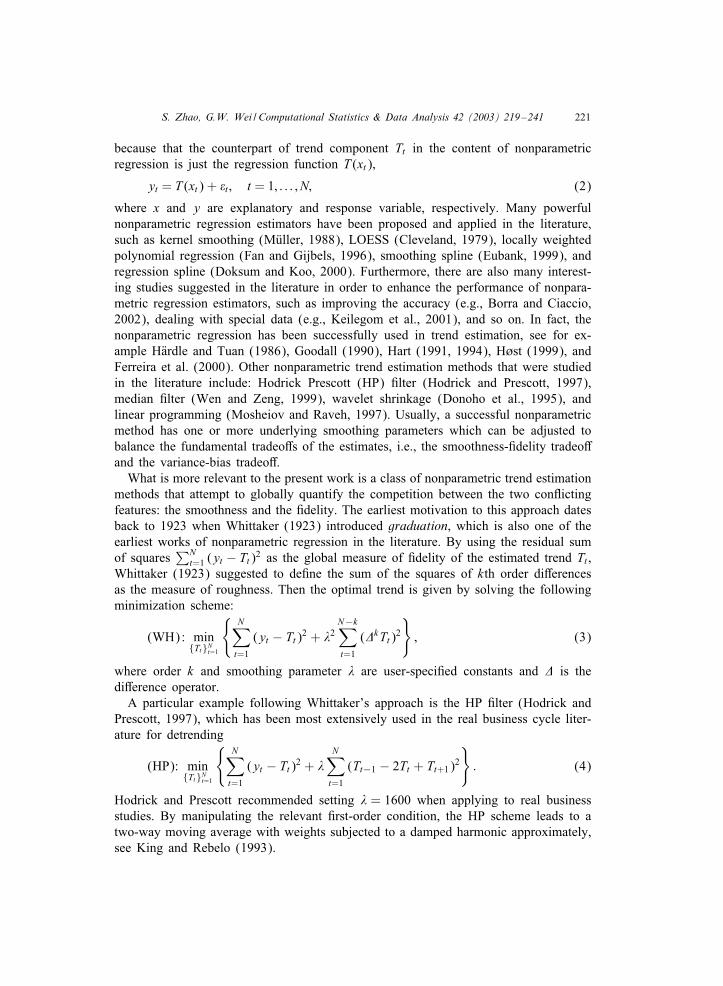
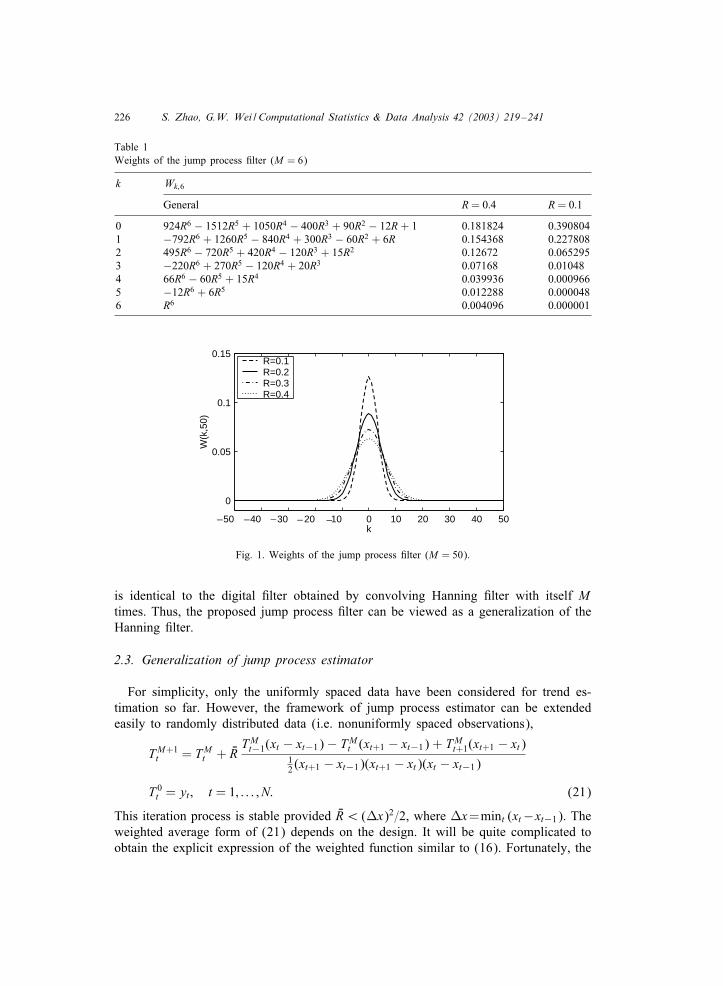
The weight assignment of the jump process 0lter is analogous to that of other kernelregression methods. When M is not too small, and for any reasonable choice of R,such as 0:16R¡ 0:5, the greater of the weights is assigned to the points close yi,the smaller weight will be assigned to the points far away from yi, see Table 1 andFig. 1. It can also be seen from the 0gure that, when M is large, although the involvedneighborhood is large, the e2ective window size of signi0cant nonzero 0lter coeScientsis smaller than 2M + 1.
A simple moving average 0lter can be formed by convolving ( 12 ;
12 ) with itself 2M
times. When M = 1, such a 0lter is the so-called Hanning 0lter (see Goodall, 1990)
(W−1; W0; W1) = ( 14 ;
12 ;
14 ): (20)
By setting R = 14 in Eq. (14), it is clear that the one step jump process 0lter has the
same coeScients as those of the Hanning 0lter and the M step jump process 0lter
226 S. Zhao, G.W. Wei / Computational Statistics & Data Analysis 42 (2003) 219–241
Table 1Weights of the jump process 0lter (M = 6)
k Wk;6
General R = 0:4 R = 0:1
0 924R6 − 1512R5 + 1050R4 − 400R3 + 90R2 − 12R + 1 0:181824 0:3908041 −792R6 + 1260R5 − 840R4 + 300R3 − 60R2 + 6R 0:154368 0:2278082 495R6 − 720R5 + 420R4 − 120R3 + 15R2 0:12672 0:0652953 −220R6 + 270R5 − 120R4 + 20R3 0:07168 0:010484 66R6 − 60R5 + 15R4 0:039936 0:0009665 −12R6 + 6R5 0:012288 0:0000486 R6 0:004096 0:000001
50 40 30 20 10 0 10 20 30 40 50
0
0.05
0.1
0.15
k
W(k
,50)
R=0.1R=0.2R=0.3R=0.4
____ _
Fig. 1. Weights of the jump process 0lter (M = 50).
is identical to the digital 0lter obtained by convolving Hanning 0lter with itself Mtimes. Thus, the proposed jump process 0lter can be viewed as a generalization of theHanning 0lter.
2.3. Generalization of jump process estimator
For simplicity, only the uniformly spaced data have been considered for trend es-timation so far. However, the framework of jump process estimator can be extendedeasily to randomly distributed data (i.e. nonuniformly spaced observations),
TM+1t = TM
t + URTMt−1(xt − xt−1) − TM
t (xt+1 − xt−1) + TMt+1(xt+1 − xt)
12 (xt+1 − xt−1)(xt+1 − xt)(xt − xt−1)
T 0t = yt; t = 1; : : : ; N: (21)
This iteration process is stable provided UR¡ (Vx)2=2, where Vx=mint (xt−xt−1). Theweighted average form of (21) depends on the design. It will be quite complicated toobtain the explicit expression of the weighted function similar to (16). Fortunately, the
S. Zhao, G.W. Wei / Computational Statistics & Data Analysis 42 (2003) 219–241 227
regression estimates based on the iterative jump process (21) can be easily obtained.Therefore, the trend estimation based on jump process (21) will be useful even if eithersome data points are missing or a cross validation method is employed.
It is well known that the continuous counterpart of the jump process in stochasticprocesses is the di2usion process, which is usually represented in the form of a partialdi2erential equation,
@T (x; �)@�
= ∇2T (x; �);
T (x; 0) = y(x): (22)
Here, the temporal variable � is the continuous time, rather than the time variableof the time series. To numerically simulate the di2usion process on uniformly spaceddata, the second-order central di2erence and explicit Euler scheme may be employedfor spatial and temporal discretizations
TM+1t = TM
t +V�
(Vx)2 (TMt−1 − 2TM
t + TMt+1);
T 0t = yt; t = 1; : : : ; N: (23)
It is interesting to note that if one sets R=V�=(Vx)2, discretized approximation scheme(23) is the same as the iterative jump process (7) and the stability of explicit Eulerscheme also requires mesh ratio V�=(Vx2)¡ 1=2. Thus, the di2usion Eq. (22) is ca-pable of providing alternative perspective for the understanding of the jump processestimator. For example, the nonuniform jump process (21) can be easily derived fromthe heat Eq. (22). Obviously, high-order spatiotemporal discretization of Eq. (22) canalso be used to construct a family of jump processes.
2.4. Jump process and Wiener process
For an appropriate range of R (0¡R¡ 1=2), the coeScients of (14), i.e. (R; 1 −2R; R), are nonnegative and R + (1 − 2R) + R = 1. Therefore, these coeScients maybe interpreted as probabilities. Consider a particle at position k on the x-axis at time� = MV�, in the next V� time period, the particle can have only three possible states:forward Vk, backward Vk, no change in position, with probabilities of P+, P− andP, respectively,
Vk =
Vx with probability P+ = R;
0 with probability P = 1 − 2R;
−Vx with probability P− = R;
(24)
where k + Vk is the particle position after V�. The process (24) is usually called ajump process in the stochastic process analysis, see for example Cox and Ross (1976).If a particle follows the jump process (24) and starts at the origin of the x-axis at� = 0, after M steps, it is easy to prove that the probability of this particle at positionk is exactly the weight W (k;M) given by (16). Hence, further investigation of jumpprocess (24) will provide considerable insight into the proposed jump process 0lter.
228 S. Zhao, G.W. Wei / Computational Statistics & Data Analysis 42 (2003) 219–241
It is obvious that the local mean and variance of Vk in (24) are
E{Vk} = Vx(P+ − P−) = 0
Var{Vk} = Vx2(P+ + P−) − (E{Vk})2
= 2Vx2R
= 2V�: (25)
In the continuum limit of an in0nitesimally small step size, the discrete model (24)yields
dk =√
2 dZ; (26)
where dZ is a standard Wiener process with E{dZ}= 0, Var{dZ2}= d�. This impliesthat the dk is also a one-dimensional Wiener process (Brownian motion without thedrift). Hence, the increase of particle movement during a relatively long period of time� is given by
k(�) − k(0) =M∑t=1
�t√
2 d�; (27)
where the �t (t = 1; 2; : : : ; M) are random numbers drawn from a standardized normaldistribution. Consequently, it can be shown that k(�) − k(0) is normally distributedwith (Hull, 1999, Section 10.2)
E{k(�) − k(0)} = 0;
Var{k(�) − k(0)} =√
2�: (28)
Here k(0) = 0 and k(�) = k. This means that under the jump process (24), the particlemovement will follow the normal distribution in the continuum limit V� → 0. SinceV� → 0 is equivalent to M → ∞ when � is 0xed, and the particle movement probabilityfunction is exactly the weight function W (k;M). One can conclude that the weightfunction W (k;M) of the proposed jump process 0lter will approach the normal kernelat the limit of M → ∞.
It is well known that the 0lter coeScients generated by convolving Hanning movingaverage 0lter approximate the Gaussian kernel as M → ∞. The above 0nding indicatesthat, the present generalized Hanning 0lter, the jump process 0lter, shares the sameproperty. Such property endows the jump process weight function to be a good kernelfunction for kernel regression, for which a widely used kernel is the Gaussian density.The proposed jump process weight function provides a discrete approximation to theGaussian kernel. On the other hand, as pointed out in the DSP literature (such as Koen-derink, 1984; Hummel, 1987), the solution of the heat di2usion Eq. (22) may equiva-lently be viewed as the result obtained by convolving original signal with the Gaussiankernel. This again agrees with the present 0nding about the jump process estimator.
2.5. Implementation particulars
It follows from above discussion that there are two simple and controllable waysto implement the jump process trend estimation. One way is based on iterative jump
S. Zhao, G.W. Wei / Computational Statistics & Data Analysis 42 (2003) 219–241 229
process (7). The time series {yt} is used as the input data. The iteration number M isused to control the 0nal estimates. The other way is to use the weighted average form(15). The trend is estimated by convolving yt and the jump process kernel once. In bothways, the R can be 0xed and only M needs to be adjusted. Theoretically, the estimatedtrends from two ways are the same, however, there are some minor di2erences dueto possible di2erent boundary treatment and applicability. Generally speaking, for uni-form spacing data trend estimation problems, the convolution implementation is moreeScient than iterative implementation. However, the iterative implementation can beeasily done for randomly spaced data regression, for which the weight kernel of theform of (15) is diScult to be constructed.
Another di2erence of these two implementations is the di2erent possible modi0cationin dealing with boundary e2ect. The boundary e2ect is a common thorny problemfor linear 0ltering and kernel smoothing, i.e., linear symmetric 0lters fail to provideestimates for the initial or=and end terms of the series (Kendall et al., 1983). Theproblem seems to be more serious in a convolution, since a larger computational supportwill locate outside the boundaries in this case, while there is only one point outsideeach boundary for the iterative way at each iteration step.
In the literature, there are some alternative approaches for dealing with bound-ary e2ect (Goodall, 1990). One approach uses progressively more asymmetric ver-sions of 0lters at the end points, it will result in more biased estimates. Such tech-niques were widely used in moving average 0ltering and kernel smoothing, see forexample Gasser and MNuller (1979), and can be directly adopted by the convolu-tion implementation of the jump process estimation. The counterpart of such a tech-nique in an iterative implementation is the well-known upwind di2erence approxi-mation scheme in numerical analysis. However, though based on the same motiva-tion, these two modi0cations along with two implementations generally yield di2erentestimates.
Arti0cially “padding data” or extrapolating the series is another approach for gener-ating necessary support for the symmetric 0lter. According to the observed character-istic of trend component, repeating the latest observation, symmetric or antisymmetricextension may be used. The same extension technique, such as symmetric or antisym-metric, can be adopted by both convolution and iterative implementations. Furthermore,it can be proved that by using the same symmetric=antisymmetric extension technique,the 0nal estimates of two di2erent implementations of the jump process are identi-cal. Therefore, we limit our attention in the present study to the implementation ofconvolution with boundary extensions.
3. Numerical experiments
3.1. Real time series analysis
The e2ect of varying the smoothing parameter M on the estimated trend is studied.A real time series, the ‘Sales of Company X’ series, is employed in the present work.Such a series is a well-known test case, see Chat0eld and Prothero (1973), Box and
230 S. Zhao, G.W. Wei / Computational Statistics & Data Analysis 42 (2003) 219–241
0 20 40 60 800
200
400
600
800 M=1
0 20 40 60 800
200
400
600
800 M=8
0 20 40 60 800
200
400
600
800 M=16
0 20 40 60 800
200
400
600
800 M=30
0 20 40 60 800
200
400
600
800 M=38
0 20 40 60 800
200
400
600
800 M=50
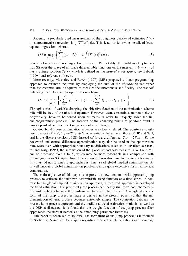
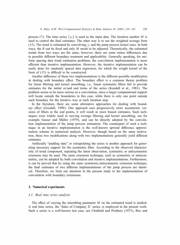
Fig. 2. Trend estimated by using the jump process as a function of M . The Chat0eld–Prothero case study:“Sales of Company X”.
Jenkins (1973), and Mosheiov and Raveh (1997). This test case is a monthly seriesranging from January 1965 to May 1971. The time series is relatively regular, witha monotonic growing trend and clearly identi0able seasonal component. Seasonallyadjusted series, which is obtained by using the X-12-ARIMA of Findley et al. (1998),is used to convolve with the jump process weight kernel, and the symmetric extensionis employed at boundaries.
The value of M is varied from 1 to 50 with a 0xed value of R (R = 0:4). As onemay expect, estimates with large smoothing parameters are very smooth, while forsmall values of M the estimates still contain high frequency components, see Fig. 2.It can be seen clearly from Fig. 2, the slope of the trend changes around the 28thobservation. This agrees with the 0nding by Mosheiov and Raveh (1997). However,when M becomes larger and larger, the estimated trend fails to provide relatively rea-sonable tendency at the right boundary due to the boundary e2ect. Two other boundarymodi0cations are also tested in this case study. One is to multiply the jump processkernel by appropriate linear functions to generate progressively more asymmetric ker-

S. Zhao, G.W. Wei / Computational Statistics & Data Analysis 42 (2003) 219–241 231
nels near the boundaries, see Gasser and MNuller (1979) for the details about such amodi0cation. Another is to use the upwind di2erence approximation along with aniterative implementation. However, these results are not as good as the present sym-metric extension. We argue that one cannot look forward to obtaining better resultsby using other boundary modi0cations, since, all modi0cations rely on a one-sidedapproximation, which inherently introduces serious bias.
For a pre-0xed R, the choice of fundamental tradeo2 indicator M is obviously acrucial decision. The optimal M is clearly determined by the signal to noise ratio inthe data. However, the practical choice of R is usually dominated by the preferencesof the practitioner or by the question being asked. The visually best principle is usedas the guideline to estimate the trend here and such an estimated trend reLects ournatural preference for the trend, viz. the estimates are smooth enough to indicate somelong-run tendency. In this test case, M = 30 is chosen as the approximate optimalsmoothing parameter.
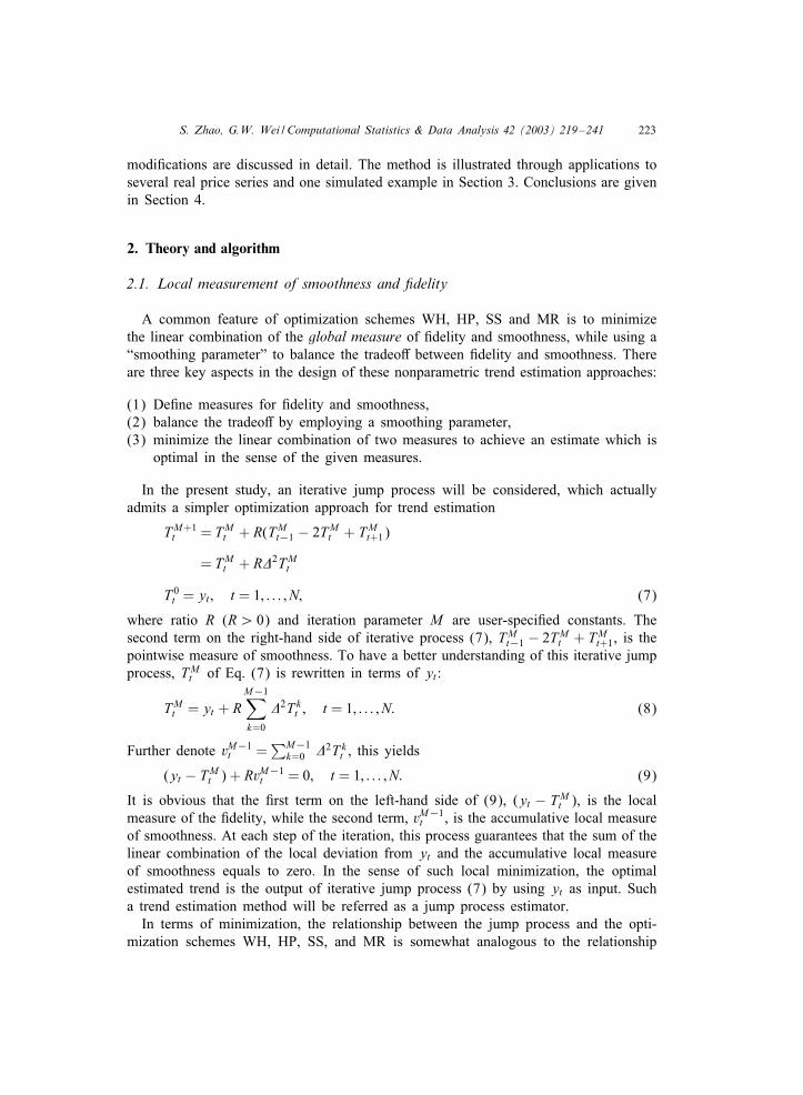
To validate the proposed jump process estimator further, a well studied economicseries, the Spanish Industrial Production Index for Energy (see Ferreira et al., 2000),is employed. The time series consists of monthly data of the IPI for energy fromJanuary 1975 up to December 1993. Although this series is somewhat more irregularthan the previous studied series, nonmonotonic trend and seasonal components are stillidenti0able from time series, see Fig. 3(a). Again, the seasonally adjusted series by theX-12-ARIMA is used as input.
The X-12-ARIMA (Findley et al., 1998) is the most commonly used method ofseasonal adjustment for oScial statistics throughout the world. Besides seasonal ad-justment, it also can present trend estimates by employing the Henderson 0lter (seeKenny and Durbin, 1982; Blanchi et al., 1999). For the IPI series, the trend estimatedby the X-12-ARIMA with default variable trend cycle routine is shown in Fig. 3(a).Visually, this estimate is not smooth enough to indicate some long-run tendency. Thissuggests that the band-width of the Henderson 0lter should be increased. To studyestimates of large band-width, the symmetric Henderson 0lter is independently imple-mented in the present study. For a comparison, the implementation of the Henderson0lter is the same as that of the jump process 0lter, i.e, the antisymmetric and symmetricextensions are employed at left and right boundaries, respectively. The trend estimatesof both the Henderson and jump process 0lters are also depicted in Fig. 3(a). It isclear that the results of two estimates are almost the same, and capture the underlyingtendency.
The estimated trend, T t , allows us to estimate the annual underlying growth of theSpanish IPI for energy, which is an issue of interest in economics. The estimate tounderlying growth, ct , can be calculated by accumulating the last 12 basic growths(Ferreira et al., 2000),
ct = [L0 + L1 + · · · + L11]VT t ; (29)
where L denotes a lag operator. The estimates of the underlying growth based on theprevious estimated trends are plotted in Fig. 3(b). It can be seen from the 0gure thatthe estimate of the X-12-ARIMA is not a smooth curve, and oscillates quite frequently,while the estimates of the Henderson and the jump process 0lters can indicate a pattern

232 S. Zhao, G.W. Wei / Computational Statistics & Data Analysis 42 (2003) 219–241
0 50 100 150 20050
60
70
80
90
100
110
120Series X_12_ARIMA Henderson Jump process
0 50 100 150 200
_5
0
5
10
X_12_ARIMA Henderson Jump process
(a)
(b)
Fig. 3. Estimation of the Spanish IPI for energy: (a) estimated trend by using the X-12-ARIMA, Henderson0lter (M = 40), and jump process 0lter (R = 0:4 and M = 100), (b) estimated annual underlying growth.
which is similar to that of Ferreira et al. (2000), thus could be interpretable from thepoint of view of economics.
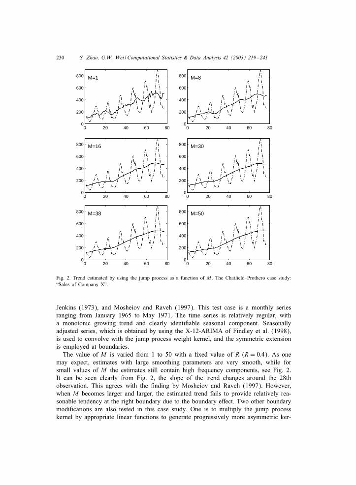
Finally, the jump process 0lter is tested by using another well studied case. This timeseries consists of the Beveridge index (Beveridge, 1921) of wheat prices from the year1500–1869 (Anderson, 1971; Hart, 1991, 1994). These data are an annual index ofprices at which wheat was sold in European markets. To correct for heteroscedasticityin the original series, a logarithmic transformation is employed. The chart (Fig. 4)clearly indicates that the transformed series consists of a nonstationary trend and aconstant variance random noise. There is no regular cyclical component presented intime series. The estimated results are depicted in Fig. 4. Here the smoothing parametersare chosen as M = 48 for the Henderson 0lter, and as R = 0:4 and M = 120 for thejump process 0lter. The symmetric extension is used at boundaries for both 0ltering.It can be seen from Fig. 4, estimates of two 0lters are almost identical, and describethe most slowly changing part of the series.
S. Zhao, G.W. Wei / Computational Statistics & Data Analysis 42 (2003) 219–241 233
1500 1550 1600 1650 1700 1750 1800 18502.5
3
3.5
4
4.5
5
5.5
Series Henderson Jump process
Fig. 4. Trend estimated by using the Henderson 0lter (M = 48) and the jump process 0lter (R = 0:4 andM = 120) for the Beveridge wheat price index data.
3.2. Simulation study
For a quantitative test of the proposed jump process estimator, a simulation studyis considered. To this end, a simple model is constructed which is analogous to theadditive model in the absence of seasonal component
y(x) = T (x) + �(x); (30)
where T (x) is a polynomial trend given by (Hart and Wehrly, 1986; HHst, 1999)
T (x) = " + 10x3 − 15x4 + 6x5; (31)
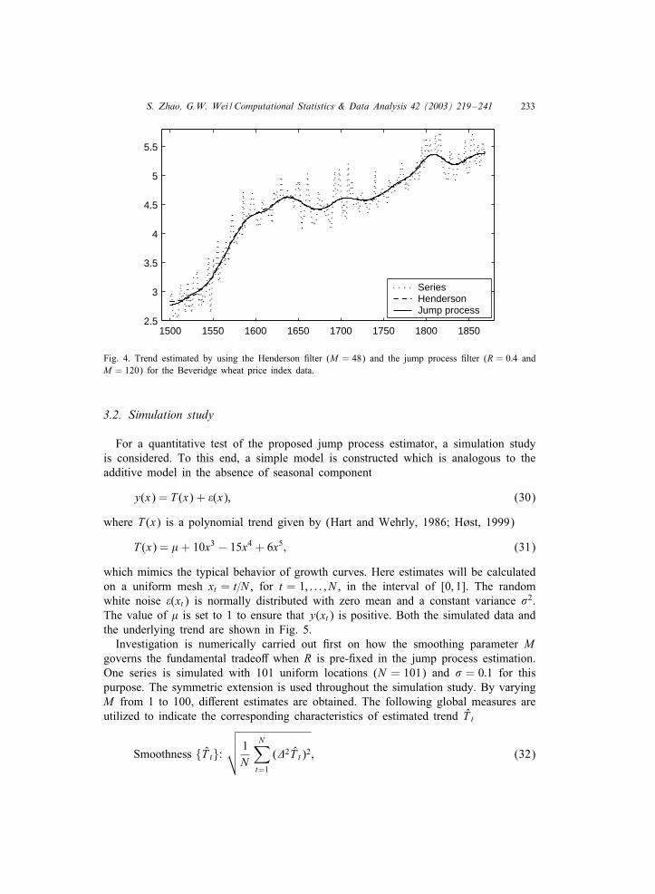
which mimics the typical behavior of growth curves. Here estimates will be calculatedon a uniform mesh xt = t=N , for t = 1; : : : ; N , in the interval of [0; 1]. The randomwhite noise �(xt) is normally distributed with zero mean and a constant variance #2.The value of " is set to 1 to ensure that y(xt) is positive. Both the simulated data andthe underlying trend are shown in Fig. 5.
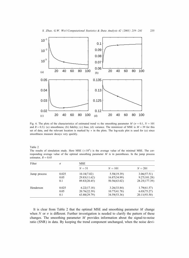
Investigation is numerically carried out 0rst on how the smoothing parameter Mgoverns the fundamental tradeo2 when R is pre-0xed in the jump process estimation.One series is simulated with 101 uniform locations (N = 101) and # = 0:1 for thispurpose. The symmetric extension is used throughout the simulation study. By varyingM from 1 to 100, di2erent estimates are obtained. The following global measures areutilized to indicate the corresponding characteristics of estimated trend T t
Smoothness {T t}:
√√√√ 1N
N∑t=1
(�2T t)2; (32)
234 S. Zhao, G.W. Wei / Computational Statistics & Data Analysis 42 (2003) 219–241
0 0.2 0.4 0.6 0.8 1
1
1.2
1.4
1.6
1.8
2
trend simulated series
Fig. 5. Plot of simulated series and trend component (noise standard deviation # = 0:1 and sample sizeN = 101).
Fidelity {T t}:
√√√√ 1N
N∑t=1
(yt − T t)2; (33)
Bias {T t}: E{|Tt − T t |}: (34)
The results are shown in Fig. 6. These numerical results verify our aforementionedtheoretical investigation, viz. when R is pre-0xed, M governs the smoothness-0delitytradeo2 and the bias-variance tradeo2.
The problem of optimal trend estimation is considered next. With a constructed trend,mean square error (MSE) is employed to measure the deviation of the numericallyestimated trend from the true trend
MSE =1N
N∑t=1
(Tt − T t)2: (35)
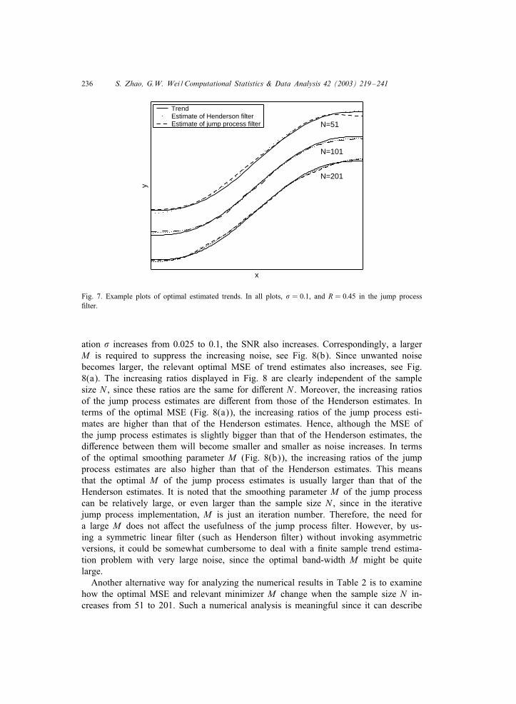
Three noise levels, # = 0:025; 0:05; 0:1, and three sample sizes, N = 51; 101, and 201are investigated. For each combination of N and #, 100 independent sets of data aregenerated. Both the jump process and Henderson 0lters are tested. Goodness-of-0t testsare employed to search for an optimal smoothing parameter which minimizes MSE inall cases. The results of simulation study are summarized in Table 2. As can be seenfrom the table, the average value of the minimal MSE is smaller than 1:0×10−3 in allcases. In other words, the satisfactory trend estimates can be obtained by using boththe Henderson and jump process 0lters in all parameter combinations. The optimalestimated trend is actually very close to the true underlying trend, see example plotsin Fig. 7. Another observation from Table 2 is that the optimal MSE of the Hendersonestimates is commonly smaller than those of the jump process estimates. However, suchdi2erence is very small, especially when sample size N is large. Visually, the di2erencebetween the estimates of the Henderson and jump process 0lters is negligible whenN = 201, see Fig. 7.
S. Zhao, G.W. Wei / Computational Statistics & Data Analysis 42 (2003) 219–241 235
20 40 60 80 100
103
10 2
10 1
(a) 20 40 60 80 1000.06
0.07
0.08
0.09
0.1
(b)
20 40 60 80 1000.02
0.03
0.04
0.05
(c) 20 40 60 80 1000.12
0.125
0.13
0.135
(d)
_
_
_
Fig. 6. The plots of the characteristics of estimated trend vs the smoothing parameter M (# = 0:1, N = 101and R = 0:3): (a) smoothness; (b) 0delity; (c) bias; (d) variance. The minimizer of MSE is M = 39 for thisset of data, and the relevant location is marked by ∗ in the plots. The log-scale plot is used for (a) sincesmoothness measure decays very quickly.
Table 2The results of simulation study. Here MSE (×105) is the average value of the minimal MSE. The cor-responding average value of the optimal smoothing parameter M is in parentheses. In the jump processestimator, R = 0:45
Filter # MSE
N = 51 N = 101 N = 201
Jump process 0:025 10.18(7.02) 5.58(19.39) 3.06(57.51)0:05 29.83(11.62) 16.87(34.99) 9.27(101.28)0:1 89.83(20.45) 50.56(63.02) 28.25(177.39)
Henderson 0:025 6.22(17.18) 3.26(33.84) 1.79(61.57)0:05 20.76(22.39) 10.77(41.78) 6.03(75.27)0:1 63.80(29.79) 34.59(53.36) 20.11(93.50)
It is clear from Table 2 that the optimal MSE and smoothing parameter M changewhen N or # is di2erent. Further investigation is needed to clarify the pattern of thesechanges. The smoothing parameter M provides information about the signal-to-noiseratio (SNR) in data. By keeping the trend component unchanged, when the noise devi-
236 S. Zhao, G.W. Wei / Computational Statistics & Data Analysis 42 (2003) 219–241
x
y
N=201
N=101
N=51
Trend Estimate of Henderson filter Estimate of jump process filter
Fig. 7. Example plots of optimal estimated trends. In all plots, # = 0:1, and R = 0:45 in the jump process0lter.
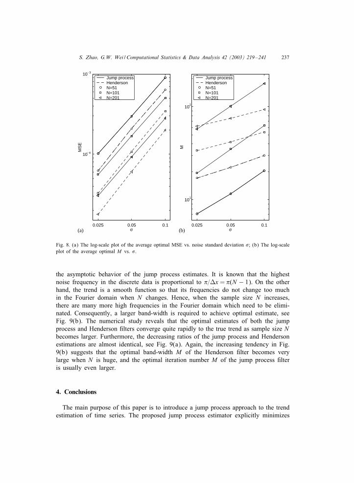
ation # increases from 0:025 to 0:1, the SNR also increases. Correspondingly, a largerM is required to suppress the increasing noise, see Fig. 8(b). Since unwanted noisebecomes larger, the relevant optimal MSE of trend estimates also increases, see Fig.8(a). The increasing ratios displayed in Fig. 8 are clearly independent of the samplesize N , since these ratios are the same for di2erent N . Moreover, the increasing ratiosof the jump process estimates are di2erent from those of the Henderson estimates. Interms of the optimal MSE (Fig. 8(a)), the increasing ratios of the jump process esti-mates are higher than that of the Henderson estimates. Hence, although the MSE ofthe jump process estimates is slightly bigger than that of the Henderson estimates, thedi2erence between them will become smaller and smaller as noise increases. In termsof the optimal smoothing parameter M (Fig. 8(b)), the increasing ratios of the jumpprocess estimates are also higher than that of the Henderson estimates. This meansthat the optimal M of the jump process estimates is usually larger than that of theHenderson estimates. It is noted that the smoothing parameter M of the jump processcan be relatively large, or even larger than the sample size N , since in the iterativejump process implementation, M is just an iteration number. Therefore, the need fora large M does not a2ect the usefulness of the jump process 0lter. However, by us-ing a symmetric linear 0lter (such as Henderson 0lter) without invoking asymmetricversions, it could be somewhat cumbersome to deal with a 0nite sample trend estima-tion problem with very large noise, since the optimal band-width M might be quitelarge.
Another alternative way for analyzing the numerical results in Table 2 is to examinehow the optimal MSE and relevant minimizer M change when the sample size N in-creases from 51 to 201. Such a numerical analysis is meaningful since it can describe
S. Zhao, G.W. Wei / Computational Statistics & Data Analysis 42 (2003) 219–241 237
0.025 0.05 0.1
10 4
10_ 3
σ
MS
EJump processHenderson N=51 N=101 N=201
0.025 0.05 0.1
101
102
σ
M
Jump processHenderson N=51 N=101 N=201
(b)(a)
_
Fig. 8. (a) The log-scale plot of the average optimal MSE vs. noise standard deviation #; (b) The log-scaleplot of the average optimal M vs. #.
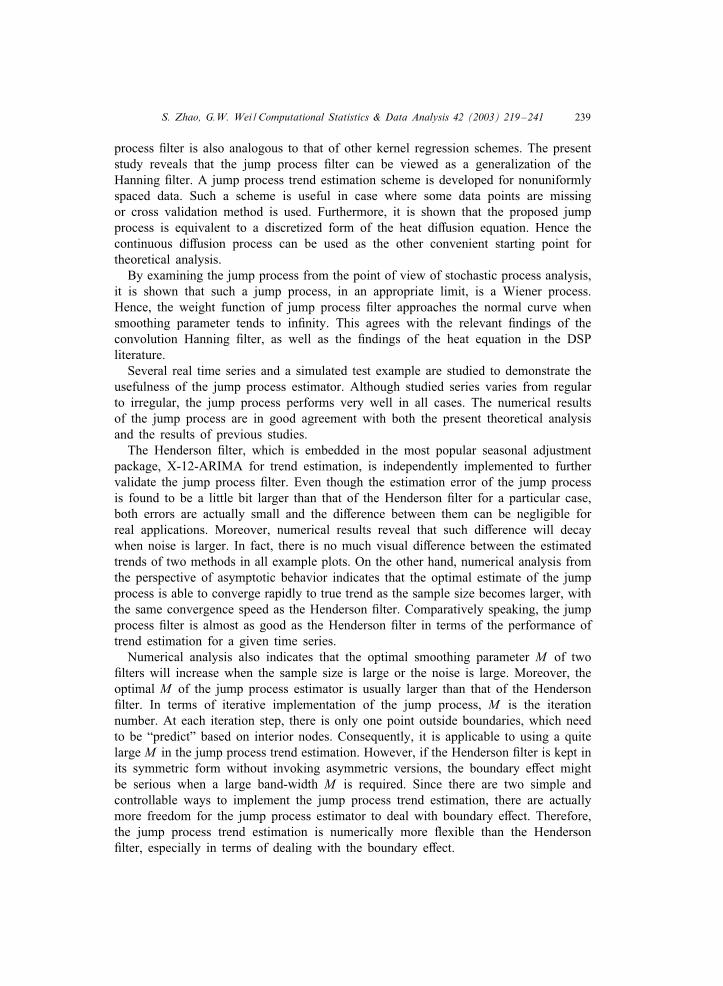
the asymptotic behavior of the jump process estimates. It is known that the highestnoise frequency in the discrete data is proportional to $=Vx = $(N − 1). On the otherhand, the trend is a smooth function so that its frequencies do not change too muchin the Fourier domain when N changes. Hence, when the sample size N increases,there are many more high frequencies in the Fourier domain which need to be elimi-nated. Consequently, a larger band-width is required to achieve optimal estimate, seeFig. 9(b). The numerical study reveals that the optimal estimates of both the jumpprocess and Henderson 0lters converge quite rapidly to the true trend as sample size Nbecomes larger. Furthermore, the decreasing ratios of the jump process and Hendersonestimations are almost identical, see Fig. 9(a). Again, the increasing tendency in Fig.9(b) suggests that the optimal band-width M of the Henderson 0lter becomes verylarge when N is huge, and the optimal iteration number M of the jump process 0lteris usually even larger.
4. Conclusions
The main purpose of this paper is to introduce a jump process approach to the trendestimation of time series. The proposed jump process estimator explicitly minimizes

238 S. Zhao, G.W. Wei / Computational Statistics & Data Analysis 42 (2003) 219–241
51 101 201
10
10 3
N
MS
EJump processHenderson σ=0.025σ=0.05 σ=0.1
51 101 201
101
102
N
M
Jump processHenderson σ=0.025σ=0.05 σ=0.1
_
4_
(b)(a)
Fig. 9. (a) The log-scale plot of the average optimal MSE vs. sample size N , (b) The log-scale plot of theaverage optimal M vs. N .
the local smoothness and 0delity of a time series. A weighted average form of thejump process estimates is derived. The connection of the proposed approach to theHanning 0lter, Gaussian kernel regression, the heat equation and the Wiener processis discussed in detail. The proposed method is validated by using both real data setsand a simulated time series.
Several trend estimation methods were successfully developed in the literature toquantify the competition between the smoothness and 0delity globally. In contrast, ajump process, which can locally minimize both features and explicitly balance thefundamental tradeo2 between them, is proposed. The investigation opens up the oppor-tunity for developing other new trend estimation methods which are optimal in a localsense. The feasibility, property, advantage and disadvantage of the trend estimationmethod development based on local optimization deserves further investigations.
The characteristic of the jump process estimator is its local optimization. In terms ofminimization, the relationship between the jump process approach and traditional meth-ods is analogous to the relationship between the collocation and Galerkin approximationin numerical analysis. The numerical strengths of the jump process are simplicity androbustness.
Like many nonparametric approaches, the estimate of the jump process also permits aweighted average form, which is very useful numerically. The weight shape of the jump
S. Zhao, G.W. Wei / Computational Statistics & Data Analysis 42 (2003) 219–241 239
process 0lter is also analogous to that of other kernel regression schemes. The presentstudy reveals that the jump process 0lter can be viewed as a generalization of theHanning 0lter. A jump process trend estimation scheme is developed for nonuniformlyspaced data. Such a scheme is useful in case where some data points are missingor cross validation method is used. Furthermore, it is shown that the proposed jumpprocess is equivalent to a discretized form of the heat di2usion equation. Hence thecontinuous di2usion process can be used as the other convenient starting point fortheoretical analysis.
By examining the jump process from the point of view of stochastic process analysis,it is shown that such a jump process, in an appropriate limit, is a Wiener process.Hence, the weight function of jump process 0lter approaches the normal curve whensmoothing parameter tends to in0nity. This agrees with the relevant 0ndings of theconvolution Hanning 0lter, as well as the 0ndings of the heat equation in the DSPliterature.
Several real time series and a simulated test example are studied to demonstrate theusefulness of the jump process estimator. Although studied series varies from regularto irregular, the jump process performs very well in all cases. The numerical resultsof the jump process are in good agreement with both the present theoretical analysisand the results of previous studies.
The Henderson 0lter, which is embedded in the most popular seasonal adjustmentpackage, X-12-ARIMA for trend estimation, is independently implemented to furthervalidate the jump process 0lter. Even though the estimation error of the jump processis found to be a little bit larger than that of the Henderson 0lter for a particular case,both errors are actually small and the di2erence between them can be negligible forreal applications. Moreover, numerical results reveal that such di2erence will decaywhen noise is larger. In fact, there is no much visual di2erence between the estimatedtrends of two methods in all example plots. On the other hand, numerical analysis fromthe perspective of asymptotic behavior indicates that the optimal estimate of the jumpprocess is able to converge rapidly to true trend as the sample size becomes larger, withthe same convergence speed as the Henderson 0lter. Comparatively speaking, the jumpprocess 0lter is almost as good as the Henderson 0lter in terms of the performance oftrend estimation for a given time series.
Numerical analysis also indicates that the optimal smoothing parameter M of two0lters will increase when the sample size is large or the noise is large. Moreover, theoptimal M of the jump process estimator is usually larger than that of the Henderson0lter. In terms of iterative implementation of the jump process, M is the iterationnumber. At each iteration step, there is only one point outside boundaries, which needto be “predict” based on interior nodes. Consequently, it is applicable to using a quitelarge M in the jump process trend estimation. However, if the Henderson 0lter is kept inits symmetric form without invoking asymmetric versions, the boundary e2ect mightbe serious when a large band-width M is required. Since there are two simple andcontrollable ways to implement the jump process trend estimation, there are actuallymore freedom for the jump process estimator to deal with boundary e2ect. Therefore,the jump process trend estimation is numerically more Lexible than the Henderson0lter, especially in terms of dealing with the boundary e2ect.

240 S. Zhao, G.W. Wei / Computational Statistics & Data Analysis 42 (2003) 219–241
Acknowledgements
This work was supported in part by the National University of Singapore.
References
Anderson, T.W., 1971. The Statistical Analysis of Time Series. Wiley, New York.Ball, M., Wood, A., 1996. Trend growth in post-1850 British economic history: the Kalman 0lter and
historical judgment. Statistician 45, 143–152.Baxter, M., King, R., 1995. Measuring business cycles: approximate band-pass 0lters for economic time
series. NBER Working Paper 5022.Beveridge, W.H., 1921. Weather and harvest cycles. Econom. J. 31, 429–452.Blanchi, M., Boyle, M., Hollingsworth, D., 1999. A comparison of methods for trend estimation. Appl.
Econom. Lett. 6, 103–109.Borra, S., Ciaccio, A.D., 2002. Improving nonparametric regression methods by bagging and boosting.
Comput. Statist. Data Anal. 38, 407–420.Box, G.E.P., Jenkins, G.M., 1973. Some comments on a paper by Chat0eld and Prothero and on a review
by Kendall. J. Roy. Statist. Soc. Ser. A 136, 337–352.Campbell, J.Y., Perron, P., 1991. Pitfalls and opportunities: what macroeconomists should know about unit
roots. NBER Macroeconom. Ann. 6, 141–201.Canova, F., 1998. Detrending and business cycle facts. J. Monetary Econom. 41, 475–512.Chat0eld, C., 1996. The Analysis of Time Series: An Introduction. Chapman & Hall, London.Chat0eld, C., Prothero, D.L., 1973. Box-Jenkins seasonal forecasting: problems in a case study J. Roy.
Statist. Soc. Ser. A 136, 295–315.Cleveland, W.S., 1979. Robust locally weighted regression and smoothing scatterplots. J. Amer. Statist.
Assoc. 74, 829–836.Cochrane, J.H., 1991. Comment to pitfalls and opportunities: what macroeconomists should know about unit
roots. NBER Macroeconom. Ann. 6, 201–210.Cox, J., Ross, S., 1976. The valuation of option for alternative stochastic processes. J. Finance Econom. 3,
145–166.Doksum, K., Koo, J.Y., 2000. On spline estimators and prediction intervals in nonparametric regression.
Comput. Statist. Data Anal. 35, 67–82.Donoho, D.L., Johnstone, I.M., Kerkyacharian, G., Picard, D., 1995. Wavelet shrinkage: asymptopia? J. Roy.
Statist. Soc. Ser. B 57, 301–369.Eubank, R.L., 1999. Nonparametric Regression and Spline Smoothing. Marcel Dekker, New York.Fan, J., Gijbels, I., 1996. Local Polynomial Modelling and its Applications. Chapman & Hall, London.Ferreira, E., N\unez-Ant\on, V., Rodr\guez-P\oo, J., 2000. Semiparametric approaches to signal extraction
problems in economic time series. Comput. Statist. Data Anal. 33, 315–333.Findley, D.F., Monsell, B.C., Bell, W.R., Otto, M.C., Chen, B.C., 1998. New capabilities and methods of
the X-12-ARIMA seasonal-adjustment program. J. Business Econom. Sat. 16, 127–177.Franses, P.H., 1998. Time Series Models for Business and Economic Forecasting. Cambridge University
Press, Cambridge.Gasser, T., MNuller, H.G., 1979. Kernel estimation of regression functions. In: Gasser, T., Rosenblatt, M.
(Eds.), Smoothing Techniques for Curve Estimation. Springer, Berlin, pp. 23–68.Goodall, C., 1990. A survey of smoothing techniques. In: Fox, J., Long, J.S. (Eds.), Modern Methods of
Data Analysis. Sage Publications, Newbury Park, CA, pp. 126–176.HNardle, W., Tuan, P.D., 1986. Some theory on M-smoothing of time series. J. Tim. Ser. Anal. 7, 191–204.Hart, J.D., 1991. Kernel regression estimation with time series errors. J. Roy. Statist. Soc. Ser. B 53, 173–187.Hart, J.D., 1994. Automated kernel smoothing of dependent data by using time series cross-validation. J.
Roy. Stat. Soc. Ser. B 56, 529–542.Hart, J.D., Wehrly, T.E., 1986. Kernel regression estimation using repeated measurement data. J. Amer.
Statist. Assoc. 81, 1080–1088.

S. Zhao, G.W. Wei / Computational Statistics & Data Analysis 42 (2003) 219–241 241
Harvey, A.C., 1989. Forecasting, Structural Time Series Models and the Kalman Filter. Cambridge UniversityPress, Cambridge.
Hodrick, R.J., Prescott, E.C., 1997. Postwar US business cycles: an empirical investigation. (Carnegie MellonUniversity, 1980) J. Money Credit Banking 29(1), 1–16.
HHst, G., 1999. Kriging by local polynomials. Comput. Statist. Data Anal. 29, 295–312.Hull, J.C., 1999. Options, Futures, and Other Derivatives. Prentice-Hall, Upper Saddle River, NJ.Hummel, A., 1987. Representations based on zero-crossing in scale-space. Proceeding IEEE Computer Vision
and Pattern Recognition Conference, pp. 204–209. In: Fischler, M.A., Firschein, O. (Eds.), Readings inComputer Vision: Issues, Problems, Principles and Paradigms. Morgan Kaufmann, Los Altos, CA.
Keilegom, I.V., Akritas, M.G., Veraverbeke, N., 2001. Estimation of the conditional distribution in regressionwith censored data: a comparative study Comput. Statist. Data Anal. 35, 487–500.
Kendall, M.G., Stuart, A., Ord, J.K., 1983. The Advanced Theory of Statistics, Vol. 3. GriSn, London.Kenny, P.B., Durbin, J., 1982. Local trend estimation and seasonal adjustment of economic and social time
series. J. Roy. Statist. Soc. Ser. A 145, 1–41.King, R.G., Rebelo, S.T., 1993. Low frequency 0ltering and real business cycles. J. Econom. Dynamics
Control 17, 207–231.Koenderink, J.J., 1984. The structure of images. Biol. Cybernet. 50, 363–370.Meade, N., Islam, T., 1995. Prediction intervals for growth curve forecasts. J. Forecasting 14, 413–430.Mills, T.C., Crafts, N.F.R., 1996. Modelling trends in economic history. Statistician 45, 153–159.Mosheiov, G., Raveh, A., 1997. On trend estimation of time series: a simple linear programming approach
J. Oper. Res. Soc. 48, 90–96.MNuller, H.-G., 1988. Nonparametric Regression Analysis of Longitudinal Data. . Lecture Notes in Statistics,
Vol. 46. Springer, Berlin.Nelson, C.R., Plosser, C., 1982. Trends and random walks in macroeconomic time series. J. Monetary
Econom. 10, 139–162.Pollock, D.S.G., 2000. Trend estimation and de-trending via rational square-wave 0lters. J. Econometrics 99,
317–334.Sims, C.A., 1988. Bayesian scepticism on unit root econometrics. J. Econom. Dynamics Control 12, 463–474.Sims, C.A., Uhlig, H., 1991. Understanding unit rooters: a helicopter tour Econometrica 59, 1591–1599.Visser, H., Molenaar, J., 1995. Trend estimation and regression analysis in climatological time series: an
application of structural time series models and the Kalman 0lter J. Climate 8, 969–979.Wei, G.W., 2000. A uni0ed approach for the solution of the Fokker–Planck equation. J. Phys. A-Math. Gen.
33, 4935–4953.Wen, Y., Zeng, B., 1999. A simple nonlinear 0lter for economic time series analysis. Econom. Lett. 64,
151–160.Whittaker, E.T., 1923. On a new method of graduation. P. Edinburgh Math. Soc. 41, 63–75.