Karel Lucas Zwetsloot

IB Candidate Number: 003738-0021

IB Physics HL

Supervisor: Rodrigo Pacios

May 2016

Internal Assessment:

Is Internal Resistance Negligible?

1

Is Internal Resistance Negligible?

Abstract

The purpose of this investigation is to evaluate to what extent the internal resistances

of power supplies are indeed negligible, as is often assumed to be true in high school problems.

For this investigation, an internal resistance is considered negligible if it makes up less than

5% of the total resistance. This resistance can be found through the use of the equation:

𝑉 = 𝜀 − 𝑅𝑖𝑛𝑡𝐼, which is derived using the basic principles of circuitry, namely Ohm’s Law.

The terminal potential difference of the circuit is measured at different values of current and

then plotted on a graph. The graph produced then displays a linear regression with y-intercept

ɛ and a gradient of -𝑅𝑖𝑛𝑡, which makes it possible to solve for the internal resistance. On top of

that, the theoretical maximum current produced by each power supply is found, to demonstrate

the impact of the internal resistance, by using: 𝐼𝑚𝑎𝑥 =𝜀

𝑅𝑖𝑛𝑡.

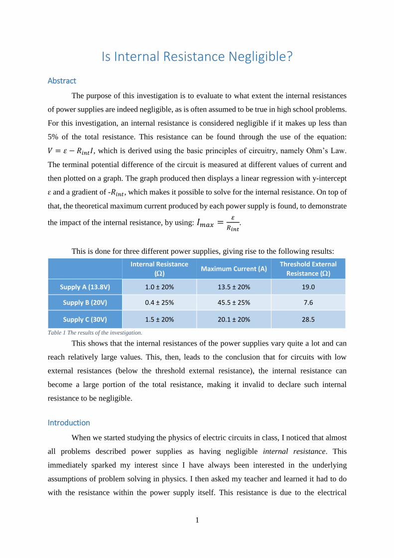
This is done for three different power supplies, giving rise to the following results:

This shows that the internal resistances of the power supplies vary quite a lot and can

reach relatively large values. This, then, leads to the conclusion that for circuits with low

external resistances (below the threshold external resistance), the internal resistance can

become a large portion of the total resistance, making it invalid to declare such internal

resistance to be negligible.

Introduction

When we started studying the physics of electric circuits in class, I noticed that almost

all problems described power supplies as having negligible internal resistance. This

immediately sparked my interest since I have always been interested in the underlying

assumptions of problem solving in physics. I then asked my teacher and learned it had to do

with the resistance within the power supply itself. This resistance is due to the electrical

Internal Resistance

() Maximum Current (A)

Threshold External

Resistance ()

Supply A (13.8V) 1.0 ± 20% 13.5 ± 20% 19.0

Supply B (20V) 0.4 ± 25% 45.5 ± 25% 7.6

Supply C (30V) 1.5 ± 20% 20.1 ± 20% 28.5

Table 1 The results of the investigation.

2

components of the power supply, which cannot have zero resistance. I was even more delighted

when I found out that the value of this resistance was something that I could actually investigate

myself. The basis of the investigation relies on the fundamental equation of circuitry, Ohm’s

Law: 𝑉 = 𝑅𝐼.

Logically, the total potential difference is equal to the electromotive force (emf) of the

power supply (𝜀), and the total resistance is equal to the sum of the external and internal

resistance. The equation can then be rewritten as: 𝜀 = (𝑅𝑒𝑥𝑡 + 𝑅𝑖𝑛𝑡)𝐼 = 𝑅𝑒𝑥𝑡𝐼 + 𝑅𝑖𝑛𝑡𝐼. Now,

it is known that 𝑅𝑒𝑥𝑡𝐼 is equal to the terminal potential difference (𝑉) of the circuit. That is, the

potential drop across the two terminals of the power supply. We can then derive the following

equation: 𝑉 = 𝜀 − 𝑅𝑖𝑛𝑡𝐼. It is interesting to note that the voltage produced by a power supply

will effectively never be equal to its emf, due to the loss of energy in the supply itself. If we

were to plot a graph of the terminal potential difference versus the current, we would expect a

linear relationship, with the emf as its y-intercept and the -𝑅𝑖𝑛𝑡 as its slope, allowing us to find

the internal resistance of the power supply, which I personally find extremely intriguing.

I then decided to investigate the internal resistances of three different power supplies,

using the above equation, to find out whether or not internal resistance is indeed negligible for

typical high school physics problems. To do this, a definition of negligible internal resistance

must be established. Since I could not clearly find such a definition, I decided to define internal

resistance to be negligible if it makes up less than 5% of the total resistance, as this seems like

a reasonable percentage to me. This definition will be used throughout this investigation.

Research Question

To what extent are the internal resistances of different power supplies indeed negligible?

Variables

Independent: The current generated (I), which is varied through adjusting the value of the

external variable resistor (R).

Dependent: The terminal potential difference (V).

Controlled:

- The same external variable resistors are used.

- The same wires are used, so that their resistance remains constant.

- The same voltmeter is used, so that its readings remain consistent with itself.

- The same ammeter is used, so that its readings remain consistent with itself.

3

Supply A (13.8V)

Supply B (20V)

Materials

- Three different power supplies

- Two variable resistors (0-10

- A voltmeter.

- An ammeter.

- A set of wires to set up the circuit.

The following power supplies, with their respective emf, are used for the experiment,

which will be referred to as supply A, B, and C accordingly:

4

Supply C (30V)

Figure 1 A diagram displaying the setup of the investigation.

Setup

The materials mentioned above should be set up according to the diagram below, which

I created myself using CircuitLab1. Note that the elements enclosed by the dashed box represent

the entire power supply. One should ensure that no wires are forming a short circuit by fixing

the wires with tape. Two resistors are used so that a greater range of values for the current can

be obtained, which improves the precision of the linear regression.

1 https://www.circuitlab.com/

5

Procedure

1. Make sure the power supply is set to the right voltage, depending on the outlet (220V

or 110V).

2. Set the variable resistors to their maximum value to ensure no overheating occurs.

3. Check if the circuit is set up exactly like the diagram above to prevent a short circuit.

4. Turn on the power supply.

5. Record the current (I) and terminal potential difference (V).

6. Vary the external resistance and record the new V-I reading.

7. Keep varying the external resistance until 10 V-I readings are obtained.

a. One should aim to obtain values of I over as wide a range as possible, depending

on the maximum current the supply can hold, to increase the precision of the

results.

8. Do not leave the current running for too long, especially at high currents, to ensure

nothing overheats.

9. Repeat steps 1-8 for the two other power supplies.

Data & Analysis

After performing the experiment, the following results were obtained for Supply A:

The uncertainty for the current is derived from the accuracy of the ammeter. The device

displayed the value of the current, which almost did not fluctuate at all, up to two decimals

places, making ± 0.01 A the appropriate uncertainty for the current. However, even though the

voltmeter displayed the value of the potential difference up to three decimals, it would not be

appropriate to use ± 0.001 V as its uncertainty. This is because the voltage measured was highly

unstable and fluctuated within a range of approximately 0.4 V. For this reason, it is much more

appropriate to use ± 0.2 V as the uncertainty for the voltage.

Using this data, a graph relating the terminal voltage and the current can be produced:

Supply A (13.8V)

Current / ± 0.01 A

0.57 0.85 1.10 1.35 1.60 1.85 2.10 2.35 2.60 2.85

Voltage / ± 0.2 V

13.4 13.1 12.8 12.5 12.3 12.2 12.0 11.6 11.3 11.0

Table 2 The raw data from Supply A.

6

y = -1.0105x + 13.955R² = 0.9915

y = -1.2174x + 14.282 y = -0.885x + 13.713

10.0

10.5

11.0

11.5

12.0

12.5

13.0

13.5

14.0

0.00 0.50 1.00 1.50 2.00 2.50 3.00

Vo

ltag

e /

±0

.2 V

Current / ± 0.01 A

Voltage vs CurrentSupply A

Trendline Max. Gradient Min. Gradient

Figure 3 The same graph as above, now with maximum and minimum gradients added to it.

From this graph, one could conclude that the internal resistance of the small power

supply equals 1.0105 Ohms, since the graph represents 𝑉 = 𝜀 − 𝑅𝑖𝑛𝑡𝐼. However, the

uncertainties of the data points should also be taken into account. This can be done by

constructing a maximum and minimum gradient using the error bars, which would represent

the upper and lower extreme of the value of the internal resistance.

y = -1.0105x + 13.955R² = 0.9915

10.0

10.5

11.0

11.5

12.0

12.5

13.0

13.5

14.0

0.00 0.50 1.00 1.50 2.00 2.50 3.00

Vo

ltag

e /

±0

.2 V

Current / ± 0.01 A

Voltage vs CurrentSupply A

Figure 2 The relationship between terminal voltage and current for Supply A.

7

y = -0.4394x + 19.226R² = 0.9939

y = -0.5525x + 19.492 y = -0.3352x + 18.905

16.5

17.0

17.5

18.0

18.5

19.0

19.5

0.50 1.00 1.50 2.00 2.50 3.00 3.50 4.00 4.50 5.00

Vo

ltag

e /

±0

.2 V

Current / ± 0.01 A

Voltage vs CurrentSupply B

Trendline Max. Gradient Min. Gradient

Figure 4 The graph relating terminal voltage and current for Supply B, including maximum and minimum gradients.

Using the minimum and maximum gradient, one could say that the internal resistance

of the power supply A falls between 0.885 and 1.2174. For this reason, one could also state the

internal resistance as 1.0 ± 0.2 or ± 20%. This allows us to effectively demonstrate

the value of the internal resistance and its degree of uncertainty.

The same process can then be applied to the two other power supplies:

Similarly, one can find the internal resistance of this power supply to be 0.4394. Using

the maximum and minimum gradient, one can determine its value with the appropriate

uncertainty: 0.4 ± 0.1 or 0.4 ± 25%.

Supply B (20V)

Current / ± 0.01 A

0.90 1.30 1.70 2.10 2.50 2.90 3.30 3.70 4.10 4.50

Voltage / ± 0.2 V

18.8 18.6 18.5 18.3 18.2 18.0 17.8 17.6 17.4 17.2

Table 3 The raw data from Supply B.

8

For supply C:

For the supply C, the internal resistance appears to be 1.4388. When taking into account

the values of the maximum and minimum gradient, one finds the internal resistance to be 1.5

± 0.3 or 1.5 ± 20%.

Conclusion

In conclusion, the internal resistances of the power supplies are larger than expected. It

is important to note that Supply C had previously been plugged into the wrong outlet (220V

instead of 110V), which caused one of its safety resistances to burn out. Even though the supply

still functions properly, the burned out component could have significantly increased its

internal resistance, which provides an explanation for its high internal resistance relative to the

Supply C (30V)

Current / ± 0.01 A

1.51 1.65 1.80 1.95 2.10 2.25 2.40 2.55 2.70 2.85

Voltage / ± 0.2 V

27.2 26.9 26.6 26.3 26.1 25.9 25.7 25.6 25.4 25.2

Table 4 The raw data from Supply C.

y = -1.4388x + 29.221R² = 0.9809

y = -1.7647x + 30.047 y = -1.2121x + 28.842

24.5

25.0

25.5

26.0

26.5

27.0

27.5

28.0

1.40 1.60 1.80 2.00 2.20 2.40 2.60 2.80 3.00

Vo

ltag

e /

±0

.2 V

Current / ± 0.01 A

Voltage vs CurrentSupply C

Trendline Max. Gradient Min. Gradient

Figure 5 The graph relating terminal voltage and current for Supply C, including maximum and minimum gradients.

9

Table 5 The results of the investigation.

other supplies. Apart from that, the differences could also be due to the physical size of the

supplies and the materials they are made of.

From the internal resistances, it is possible to calculate another interesting feature of

the power supplies: the theoretical maximum current produced, which demonstrates the effect

of the internal resistance. It is derived using the equation that was also used earlier on in the

investigation: 𝐼 =𝜀

𝑅𝑒𝑥𝑡+𝑅𝑖𝑛𝑡. This maximum current would occur when the external resistance

is zero. Therefore, it is possible to find the theoretical maximum current produced by the power

supply: 𝐼𝑚𝑎𝑥 =𝜀

𝑅𝑖𝑛𝑡. However, in real life the power supplies would not be able to withstand

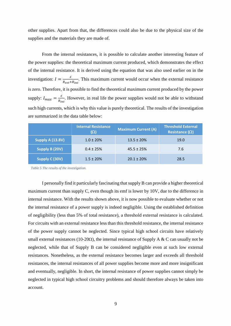
such high currents, which is why this value is purely theoretical. The results of the investigation

are summarized in the data table below:

I personally find it particularly fascinating that supply B can provide a higher theoretical

maximum current than supply C, even though its emf is lower by 10V, due to the difference in

internal resistance. With the results shown above, it is now possible to evaluate whether or not

the internal resistance of a power supply is indeed negligible. Using the established definition

of negligibility (less than 5% of total resistance), a threshold external resistance is calculated.

For circuits with an external resistance less than this threshold resistance, the internal resistance

of the power supply cannot be neglected. Since typical high school circuits have relatively

small external resistances (10-20), the internal resistance of Supply A & C can usually not be

neglected, while that of Supply B can be considered negligible even at such low external

resistances. Nonetheless, as the external resistance becomes larger and exceeds all threshold

resistances, the internal resistances of all power supplies become more and more insignificant

and eventually, negligible. In short, the internal resistance of power supplies cannot simply be

neglected in typical high school circuitry problems and should therefore always be taken into

account.

Internal Resistance

() Maximum Current (A)

Threshold External

Resistance ()

Supply A (13.8V) 1.0 ± 20% 13.5 ± 20% 19.0

Supply B (20V) 0.4 ± 25% 45.5 ± 25% 7.6

Supply C (30V) 1.5 ± 20% 20.1 ± 20% 28.5

10

Evaluation

Since the power supplies did not publish their internal resistances, there is unfortunately

no way to compare the experimental values to expected values, which makes it rather difficult

to evaluate the errors of the experiment. However, there are certain systematic errors that have

in fact affected the results of the experiment and caused the rather high percentage

uncertainties.

A major cause of the lack of precision of the results is the limited value of the current

the power supplies could withstand. The power supplies could withstand either three or five

amps at their maximum, which severely limits the range of data points that can be measured.

A greater amount and range of data points would increase the precision of the trendline, which

would ultimately lead to a greater precision in the value of the internal resistance of the power

supplies. This could possibly be resolved by using other power supplies that are able to

withstand higher values of current, increasing the possible range of data points and therefore

the overall precision of the experiment. Another way of potentially reducing this error would

be adding more variable resistors or substituting them with ones that can go up to higher

resistances. This would increase the maximum external resistance, which ultimately also

increases the range of the possible values for the current by lowering the minimum value of the

current.

Another source of error that occurred during the experiment is the heating effect of

currents. At high values of current, the resistors absorb high amounts of kinetic energy from

the electrons, which causes them to heat up. The problem with this is that as the temperature

of the resistors increases, their resistance increases as well. Due to their changing resistance,

the resistors no longer obey Ohm’s Law, making the equation the investigation is based on

invalid, which could majorly affect the results. The changing resistance occurs because at

higher temperatures the metal cations are vibrating more and are hence obstructing the free

flow of electrons by colliding more with them. Now, a changing external resistance is not a

problem in this case, since we have been doing that throughout the entire experiment and this

will only alter the value of the current. The source of error lies in the fact that the power supplies

themselves also started to become warmer. This would mean that their internal resistances were

not constant, but actually increased at higher values of current. However, this cannot have

affected the results by much, since this would have resulted in a steeper slope at the higher

11

value of current, which is not clearly visible. Nonetheless, this could possibly be improved by

collecting the data at separate moments in time, so that the current would not flow continuously

for a long period of time. This would limit the heating of the power supply and hence reduce

this source of error.

Overall, the investigation has been very successful. I personally enjoyed the process

very much and was intrigued by the final results, especially since most problems assume that

such internal resistance is in fact negligible. I found it particularly interesting that the internal

resistances of the power supplies are so different and the effect this has on their theoretical

maximum current produced. I look forward to learning more about this in the future and

perhaps investigating this with more precise measuring devices. This could possibly reduce the

uncertainty of the voltage measured, which would ultimately reduce the uncertainty of the value

of the internal resistance.