1

Distributed Interference Management Policies for Heterogeneous Small Cell Networks

Kartik Ahuja, Yuanzhang Xiao and Mihaela van der Schaar

Department of Electrical Engineering, UCLA, Los Angeles, CA, 90095

Email: ahujak@ucla.edu, yxiao@seas.ucla.edu and mihaela@ee.ucla.edu

Abstract

We study the problem of distributed interference management in a network of heterogeneous

small cells with different cell sizes, different numbers of user equipments (UEs) served, and different

throughput requirements by UEs. We consider the uplink transmission, where each UE determines when

and at what power level it should transmit to its serving small cell base station (SBS). We propose a

general framework for designing distributed interference management policies, which exploits weak

interference among non-neighboring UEs by letting them transmit simultaneously (i.e., spatial reuse),

while eliminating strong interference among neighboring UEs by letting them transmit in different time

slots. The design of optimal interference management policies has two key steps. Ideally, we need to

find all the subsets of non-interfering UEs, i.e., the maximal independent sets (MISs) of the interference

graph, but this is NP-hard (non-deterministic polynomial time) even when solved in a centralized manner.

Then, in order to maximize some given network performance criterion subject to UEs’ minimum

throughput requirements, we need to determine the optimal fraction of time occupied by each MIS,

which requires global information (e.g., all the UEs’ throughput requirements and channel gains). In

our framework, we first propose a distributed algorithm for the UE-SBS pairs to find a subset of

MISs in logarithmic time (with respect to the number of UEs). Then we propose a novel problem

reformulation which enables UE-SBS pairs to determine the optimal fraction of time occupied by each

MIS with only local message exchange among the neighbors in the interference graph. Despite the

fact that our interference management policies are distributed and utilize only local information, we

can analytically bound their performance under a wide range of heterogeneous deployment scenarios

in terms of the competitive ratio with respect to the optimal network performance, which can only

be obtained in a centralized manner with NP complexity. Remarkably, we prove that the competitive

ratio is independent of the network size. Through extensive simulations, we show that our proposed

policies achieve significant performance improvements (ranging from 150% to 700%) over state-of-the-

art policies.

I. INTRODUCTION

Dense deployment of low-cost heterogeneous small cells (e.g. picocells, femtocells) has be-

come one of the most effective solutions to accommodate the exploding demand for wireless

2

spectrum [1] [2] [3]. On one hand, dense deployment of small cells significantly shortens the

distances between small cell base stations (SBSs) and their corresponding user equipments (UEs),

thereby boosting the network capacity. On the other hand, dense deployment also shortens the

distances between neighboring SBSs, thereby potentially increasing the inter-cell interference.

Hence, while the solution provided by the dense deployment of small cells is promising, its

success depends crucially on interference management by the small cells. Efficient interference

management is even more challenging in heterogeneous small cell networks, due to the lack of

central coordinators, compared to that in traditional cellular networks.

In this paper, we propose a novel framework for designing interference management policies

in the uplink of small cell networks, which specify when and at what power level each UE

should transmit1. Our proposed design framework and the resulting interference management

policies fulfill all the following important requirements:

• Deployment of heterogeneous small cell networks: Existing deployments of small cell net-

works exhibit significant heterogeneity such as different types of small cells (picocells and

femtocells), different cell sizes, different number of UEs served, different UEs’ throughput

requirements etc.

• Interference avoidance and spatial reuse: Effective interference management policies should

take into account the strong interference among neighboring UEs, as well as the weak

interference among non-neighboring UEs. Hence, the policies should effectively avoid in-

terference among neighboring UEs and use spatial reuse to take advantage of the weak

interference among non-neighboring UEs.

• Distributed implementation with local information and message exchange: Since there is no

central coordinator in small cell networks, interference management policies need to be

computed and implemented by the UEs in a distributed manner, by exchanging only local

information through local message exchanges among neighboring UE-SBS pairs.

• Scalability to large networks: Small cells are often deployed over a large scale (e.g., in a

city). Effective interference management policies should scale in large networks, namely

achieve efficient network performance while maintaining low computational complexity.

• Ability to optimize different network performance criteria: Under different deployment sce-

1Although we focus on uplink transmissions in this paper, our framework can be easily applied to downlink transmissions.

3

narios the small cell networks may have different performance criteria, e.g., weighted

sum throughput or max-min fairness. The design framework should be general and should

prescribe different policies to optimize different network performance criteria.

• Performance guarantees for individual UEs: Effective interference management should pro-

vide performance guarantees (e.g., minimum throughput guarantees) for individual UEs.

As we will discuss in detail in Section II, existing state-of-the-art policies for interference

management cannot simultaneously fulfill all of the above requirements.

Next, we describe our key results and major contributions:

1. We propose a general framework for designing distributed interference management poli-

cies that maximizes the given network performance criterion subject to each UE’s minimum

throughput requirements. The proposed policies schedule maximal independent sets (MISs)2 of

the interference graph to transmit in each time slot. In this way, they avoid strong interference

among neighboring UEs (since neighboring UEs cannot be in the same MIS), and efficiently

exploit the weak interference among UEs in a MIS by letting them to transmit at the same time.

2. We propose a distributed algorithm for the UEs to determine a subset of MISs. The subset

of MISs generated ensures that each UE belongs to at least one MIS in this subset. Moreover,

the subset of MISs can be generated in a distributed manner in logarithmic time (logarithmic

in the number of UEs in the network) for bounded-degree interference graphs3. The logarithmic

convergence time is significantly faster than the time (linear or quadratic in the number of UEs)

required by the distributed algorithms for generating subsets of MISs in [4]–[6].

3. Given the computed subsets of MISs, we propose a distributed algorithm in which each

UE determines the optimal fractions of time occupied by the MISs with only local message

exchange. The message is exchanged only among the UE-SBS pairs that strongly interfere with

each other, i.e. among neighbors in the interference graph. The distributed algorithm will output

the optimal fractions of time for each MIS such that the given network performance criterion is

2Consider the interference graph of the network, where each vertex is a UE-SBS pair and each edge indicates strong interference

between the two vertices. An independent set (IS) is a set of vertices in which no pair is connected by an edge. An IS is a MIS

if it is not a proper subset of another IS.3Bounded-degree graphs are the graphs whose maximum degree can be bounded by a constant independent of the size of the

graph, i.e., ∆ = O(1). As we will show in Theorem 5, for the interference graphs that are not bounded-degree graphs, even

the centralized solution, given all the MISs, cannot satisfy the minimum throughput requirements.

4

maximized subject to the minimum throughput requirements.

4. Under a wide range of conditions, we analytically characterize the competitive ratio of

the proposed distributed policy with respect to the optimal network performance. Importantly,

we prove that the competitive ratio is independent of the network size, which demonstrates

the scalability of our proposed policy in large networks. Remarkably, the constant competitive

ratio is achieved even though our proposed policy requires only local information, is distributed,

and can be computed fast, while the optimal network performance can only be obtained in a

centralized manner with global information (e.g., all the UEs’ channel gains, maximum transmit

power levels, minimum throughput requirements) and NP (non-deterministic polynomial time)

complexity.

5. Through simulations, we demonstrate significant (from 160% to 700 %) performance gains

over state-of-the-art policies. Moreover, we show that our proposed policies can be easily adapted

to a variety of heterogeneous deployment scenarios, with dynamic entry and exit of UEs.

The rest of the paper is organized as follows. In Section II we discuss the related works

and their limitations. We describe the system model in Section III. Then we formulate the

interference management problem and give a motivating example in Section IV. We propose the

design framework in Section ??, and demonstrate the performance gain of our proposed policies

in Section VI. Finally, we conclude the paper in Section VII.

II. RELATED WORKS

State-of-the-art interference management policies can be divided into three main categories:

policies based on power control, policies based on spatial reuse, and policies based on joint

spatial reuse and power control.

A. Distributed Interference Management Based on Power Control

Policies based on distributed power control, with representative references [7]–[14] have been

used for interference management in both cellular and ad-hoc networks. In these policies, all the

UEs in the network transmit at a constant power all the time (provided that the system parameters

remain the same)4. The major limitation of policies based on power control is the difficulty in

4Although some power control policies [7], [8], [10] go through a transient period of adjusting the power levels before the

convergence to the optimal power levels, the users maintain constant power levels after the convergence.

5

providing minimum throughput guarantees for each UE, especially in the presence of strong

interference. Some works [7], [8], [10] use pricing to mitigate the strong interference. However,

they [7], [8], [10] cannot strictly guarantee the UEs’ minimum throughput requirements. Indeed,

the low throughput experienced by some users, caused by strong interference, is the fundamental

limitation of such power control approaches - even the optimal power control policy obtained

by a central controller [15], [16] can be inefficient 5. Since strong interference is very common

in dense small cell deployments (e.g. in offices and apartments where SBSs are installed close

to each other [18]), more efficient policies are required which can guarantee the individual

UEs’ throughput requirements. Also, there exist a different strand of work based on [19] which

proposes a distributed algorithm to achieve the desired minimum throughput requirement for each

UE. However, these works cannot optimize network performance criterion such as weighted sum

throughput, max-min fairness etc. and hence are suboptimal.

B. Distributed Spatial Reuse Based on Maximal Independent Sets

An efficient solution to mitigate strong interference is spatial reuse, in which only a subset of

UEs (which do not significantly interfere with each other) transmit at the same time. Spatial Time

reuse based Time Division Multiple Access (STDMA) has been widely used in existing works

on broadcast scheduling in multi-hop networks [4]–[6]6. Specifically, these policies construct a

cyclic schedule such that in each time slot an MIS of the interference graph is scheduled. The

constructed schedule ensures that each UE is scheduled at least once in the cycle.

In terms of performance, STDMA policies [4]–[6] cannot guarantee the minimum throughput

requirement of each UE, and usually adopt a fixed scheduling (i.e. follow a fixed order in

which the MISs are scheduled), which may be very inefficient depending on the given network

performance criteria. For example, the policies in [6] are inefficient in terms of fairness. In terms

of complexity, for the distributed generation of the subsets of MISs, the STDMA policies in [4]–

[6] require an ordering of all the UEs, and have a computational complexity (in terms of the

number of steps executed by the algorithm) that scales as O(|V |)) (in [5], [6]) or O(|V ||E|))

5In the case of average sum throughput maximization given the minimum average throughput constraints of the UEs, the

power control policies are inefficient if the feasible rate region is non-convex [17] .6These works [4]–[6] do not have the exactly same model as in our setting. However, these works can be adapted to our

model. Hence, we also compare with these works to have a comprehensive literature review.

6

(in [4]), where |V | and |E| are the number of vertices/UEs and the number of edges in the

interference graph, respectively. Hence, in large-scale dense deployments, the complexity grows

superlinearly with the number of UEs, making the policies difficult to compute. By contrast, our

proposed distributed algorithm for generating subsets of MISs does not require the ordering of

all the UEs, and has a complexity that scales as O(log |V |), namely sublinearly with the number

of the UEs, for bounded-degree graphs.7

Finally, the STDMA policies in [4]–[6] are designed for the MAC layer and assume that all

the UEs are homogeneous at the physical layer. In practice, different UEs are heterogeneous due

to their different distances from their SBSs, their different maximum transmit power levels, etc.

This heterogeneity is important, and will be considered in our design framework.

C. Distributed Power Control and Spatial Reuse For Multi-Cell Networks

As we have discussed, the works in the above two categories either focus on distributed power

control in the physical layer [7], [8], [10] or focus on distributed spatial reuse in the MAC layer

[4]–[6]. Similar to our paper, some works (representative references [20]–[24] ) adopted a cross-

layer approach and proposed distributed joint power control and spatial reuse for multi-cell

networks. However, although these works schedule a subset of UEs to transmit at the same time,

the subset is not the MIS of the interference graph [22], [23]. For example, the policies in [22],

[23] schedule one UE from each small cell at the same time, even if some UEs are from small

cells very close to each other. In this case, the UEs will experience strong inter-cell interference.

Hence, the works in [22], [23] cannot perfectly eliminate strong interference from neighboring

cells and exploit weak interference from non-neighboring cells. Moreover, the works in [20]–[24]

cannot provide minimum throughput guarantees for the UEs.

III. SYSTEM MODEL

A. Heterogeneous Network of Small Cells

We consider a heterogeneous network of K small cells operating in the same frequency

band8 (see Fig. 1), which represents a common deployment scenario considered in practice

7As will be shown in Theorem 5, for graphs which are not bounded degree graphs, even a centralized solution based on all

the MISs cannot satisfy the minimum throughput requirements.8Our solutions will be based on spatial time reuse assuming every UE uses the same frequency. Our solutions can be extended

to spatial frequency reuse, where we let different MISs operate in non-overlapping frequency bands.

7

[10] [13] [25]. Note that the small cells can be of different types (e.g. picocells, femtocells,

etc.) and thereby belong to different tiers in the heterogeneous network. Each small cell j has

one SBS, (SBS-j), which serves a set of UEs under a closed access scenario [10]. Denote

the set of UEs by U = {1, ..., N}. We write the association of UEs to SBSs as a mapping

T : {1, ..., N} → {1, .., K}, where each UE-i is served by SBS-T (i). We focus on the uplink

transmissions; the extension to downlink transmissions is straightforward when each SBS serves

one UE at a time (e.g. TDMA among UEs connected to the same SBS).

Each UE-i chooses its transmit power pi from a compact set Pi ⊆ R+. We assume that

0 ∈ Pi, ∀i ∈ {1, ..., N}, namely any UE can choose not to transmit. The joint power profile

of all the UEs is denoted by p = (p1, ...., pN) ∈ P , ΠNi=1Pi. Under the joint power profile

p, the signal to interference and noise ratio (SINR) of UE-i’s signal, experienced at its serving

SBS-j = T (i), can be calculated as γi(p) =gijpi

N∑k=1,k 6=i

gkjpk+σ2j

, where gij is the channel gain from

UE-i to SBS-j, and σ2j is the noise power at SBS j. The UEs do not cooperate to encode their

signals to avoid interference, hence, each UE-SBS pair treats the interference from other UEs

as white noise. Hence, each UE-i gets the following throughput [22], ri(p) = log2(1 + γi(p))9.

B. Interference Management Policies

The system is time slotted at t = 0,1,2..., and the UEs are assumed to be synchronized as in

[22], [23] [26] [27].. At the beginning of each time slot t, each UE-i decides its transmit power

pti and obtains a throughput of ri(pt). Each UE i’s strategy, denoted by πi : Z+ = {0, 1, ..} → Pi,

is a mapping from time t to a transmission power level pi ∈ Pi. The interference management

policy is then the collection of all the UEs’ strategies, denoted by π = (π1, ..., πN). The average

throughput for UE i is given as Ri(π) = limT→∞1

T+1

T∑t=0

ri(pt), where pt = (π1(t), ..., πN(t))

is the power profile at time t. We assume the channel gain to be fixed over the considered

time horizon as in [22] [28]–[31]. However, we will illustrate in Section VI that our framework

performs well under dynamic channel conditions (due to fading, time varying channel) as well.

An interference management policy πconst is a policy based on power control [7], [8], [10]

if πconst(t) = p for all t. As we have discussed before, our proposed policy is based on MISs

9We use the Shannon capacity here. However, our analysis is general and applies to the throughput models that consider the

modulation scheme used.

8

FBS-1

FUE-2

PUE-1 PUE-2

PBS

FBS-2

FUE-3

FUE

PUE

FBS

PBS

Femtocell User

Equipment

Picocell User

Equipment

Femtocell Base

Station

Picocell Base

Station

Direct channel

gain

Cross channel

gain

Local message exchange Local message exchange

Femto/

Pico Cell

FUE-1

Figure 1. Illustration of a heterogeneous small cell network.

of the interference graph. The interference graph G has N vertices, each of which is one of

the N UE-SBS pairs. There is an edge between two pairs/vertices if their cross interference

is high (rules for deciding if interference is high will be discussed in Section V) and let there

be M edges in the graph. Given an interference graph, we write I = {I1, ..., INMIS} as the set

of all the MISs of the interference graph. Let pIj be a power profile in which the UEs in the

MIS Ij transmit at their maximum power levels and the other UEs do not transmit, namely

pk = pmaxk , maxPk if k ∈ Ij and pk = 0 otherwise. Let PMIS = {pI1 , ...,pINMIS } be the

set of all such power profiles. Then π is a policy based on MIS if π(t) ∈ PMIS for all t. We

denote the set of policies based on MISs by ΠMIS = {π : Z+ → PMIS}.

IV. PROBLEM FORMULATION AND A MOTIVATING EXAMPLE

In this section, we formulate the interference management policy design problem and give a

motivating example to highlight the advantages of the proposed policy over existing policies.

A. The Interference Management Policy Design Problem

We aim to optimize a chosen network performance criterion W (R1(π), ...., RN(π)), defined

as a function of the UEs’ average throughput. We can choose any performance criterion that

is concave in R1(π), ...., RN(π). For instance, W can be the weighted sum of all the UEs’

throughput, i.e.N∑i=1

wiRi(π) withN∑i=1

wi = 1 and wi ≥ 0. Alternatively, the network performance

can be max-min fairness (i.e. the worst UE’s throughput) and hence W can be defined as

miniRi(π). The policy design problem can be then formalized as follows:

Policy Design Problem (PDP) maxπ W (R1(π), ..., RN(π))

subject to Ri(π) ≥ Rmini , ∀i ∈ {1, ..., N}

9

Step 1.

Each UE identifies

the interfering UE-

SBS pairs.

Step 2.

Distributed generation of MISs:

each UE executes Phase 1 and 2

to identify the MISs it belongs to.

(Theorem 1)

Step 3.

Each UE executes the procedure in

Table I, to arrive at the optimal

fraction of time allocated to each

MIS. (Theorem 2 and 3)

Step 4.

Each UE computes the cycle

length and the duration of each

MIS in the cycle.

Figure 2. Steps in the Design Framework.

The above design problem is very challenging to solve even in a centralized manner (it has

been shown to be NP-hard [32] even when we restrict to policies based on power control πconst).

Denote the optimal value of the PDP as Wopt. Our goal is to develop distributed, polynomial-time

algorithms to construct policies that achieve a constant competitive ratio with respect to Wopt,

with the competitive ratio independent of the network size. We achieve our goal by focusing

on policies based on MISs ΠMIS , among other innovations that will be described in Section V.

Next, we provide a motivating example to demonstrate the efficiency of our proposed policy.

V. DESIGN FRAMEWORK FOR DISTRIBUTED INTERFERENCE MANAGEMENT

A. Proposed Design Framework

Our proposed design framework (see Fig. 2) consists of the following four steps.

Step 1. Identification of the interfering neighbors: In Step 1, each UE-SBS pair identifies

the UE-SBS pairs that strongly interfere with it. Essentially, each pair obtains a local view (i.e.,

its neighbors) of the interference graph. Note that an edge exists between two pairs if at least

one of them identifies the other as a strong interferer.

Specifically, each UE-SBS pair is first informed of other pairs in the geographical proximity

by managing servers (e.g., femtocell controllers/gateways) [33] [34] [29] [30]. Then each pair

can decide whether another pair is strongly interfering based on various rules, such as rules

based on Received Signal Strength (RSS) in the Physical Interference Model [33] [29] [30], and

rules based on the locations in the Protocol Model [28]. If one pair identifies another pair as

strongly interfering, its decision can be relayed by the managing servers to the latter, such that

any two pairs can reach consensus of whether there exists an edge between them.

Step 2. Distributed generation of MISs that span all the UEs: In Step 2, the UE-SBS

pairs generate a subset of MISs in a distributed fashion. It is important that the generated subset

10

1 32

4C11

0 =

{R,Y,G}

C120 = {R,Y,G}

C140 = {R,Y,G}

C130 ={R,Y,G}

12

34

C12P1

= {}1 3

2

2

4

C14P1

= {Y}

C11P1

= {} C13P1

= {G}

C12P1+P2

= {}

C14P1+P2

= {}

C11P1+P2

= {} C13P1+P2

= {}

A). Before Phase 1 and Phase 2 B). After Phase 1,

(Time = P1 time slots).

C). After Phase 2,

(Time=P1+P2 time slots). C1Q

iList of colors

remaining

for UE-i at time slot

Q

Y/G/R color acquired

by a UE

Set of colors {R,G},

{R,Y} acquired by a

UE{R,Y,G} {Red,Yellow,Green}

1. Color classes corresponding to Y,G

are ISs after Phase 1, R is MIS

2. Color classes corresponding to

R,Y,G are MISs after Phase 2.

3

Figure 3. Illustration of the distributed generation of MISs in Step 2.

spans all the UEs, namely every UE is contained in at least one MIS in the subset. Otherwise,

some UEs will never be scheduled.

The key idea is that from a given list of colors, each UE has to choose a set of colors such

that the choice does not conflict with its neighbors. We should ensure that each UE has at least

one color. We call the set of UEs with the same color “a color class”. In addition, we should also

ensure that every color class is a MIS. This step is composed of two phases: first, distributed

coloring of the interference graph based on [35], and second, extension of color classes to MISs.

All the UEs are synchronized and carry out their computation simultaneously. We now explain

the algorithm in detail. The pseudo-codes can be found in Table II and III in the Appendix.

Phase 1. Distributed coloring of the interference graph: Let H10 be the maximum number

of colors given to all SBSs at the installation and di be the degree (number of neighbors in the

interference graph) of the ith pair. The goal of this phase is to let each UE-SBS pair i choose

one color from C0i , {1, ...H} ∩ {1, .., di + 1}, such that no neighbors choose the same color.

The distributed coloring works as follows.

i) At the beginning of each time slot t, each UE i chooses a color from the set of remaining

colors Cti uniformly randomly, and informs its neighbors of its tentative choice. This information

can be transmitted through the back-haul network/X2 interface that is used for ICIC [34].

ii) If the tentative choice of a UE does not conflict with any of its neighbor, then it fixes its

color choice and informs the neighbors of its choice. This UE does not contend for colors any

10The maximum number of colors H should be set to be larger than the maximum number of UE-SBS pairs interfering with

any UE-SBS pair. The SBSs can determine H according to the deployment scenario. H in general will also include the number

of UEs that use the same SBS who interfere with each other along with the other neighboring UEs. For example, H can be

10-15 in an office building with dense deployment of SBSs, and can be 3-5 in a residential area.

11

further in Phase 1. The neighbors delete the color chosen by i from their lists Ct+1j

,∀j ∈ N (i),

where N (i) is the set of i’s neighbors.

iii) Otherwise, if there is a conflict, then the UE does not choose that color and repeats i) and

ii) in the next time slot.

There are dc1 log 43Ne + 1 time slots in Phase 1, where c1 is the parameter given by the

protocol. The number of time slots is known to the SBSs at installation. Phase 1 is successful if

all the UEs acquire a color, which implies that the set of color classes (i.e., the set of UE-SBS

pairs with the same color) spans all the UEs.

Phase 2. Extending color classes to the MISs: Each color class obtained at the end of Phase

1 is an independent set (IS) of the graph. In Phase 2, we extend each of these ISs to MISs and

possibly generate additional MISs. After Phase 1, each UE has chosen one color and deleted

some colors from its list. But there may still be remaining colors in its list that are not acquired

by any of its neighbors. If the UEs can acquire these remaining colors without conflicting with

its neighbors, then each color class will be a MIS. Phase 2 works as follows.

i) At each time slot in Phase 2, UE i chooses each color from the remaining colors in its

list independently with probability c. Each UE i then sends the set of its tentative choices to its

neighboring UEs, and receives their neighbors’ choices.

ii) For any tentative choice of color, if there is a conflict with at least one neighbor, then that

color is not fixed; otherwise, it is fixed.

iii) At the end of each time slot, each UE deletes its set of fixed colors from its list, and

transmits this set of fixed colors to its neighbors, who will delete these fixed colors from their

lists as well. Note that a UE deletes a particular color if and only if the UE itself or some of

its neighbors have chosen this color. Based on this key observation, we can see that if a color

is not in any UE’s list, the set of UEs with this color is a MIS. If all the UEs have an empty

list, then for any color in the set {1, ..., H}, the set of UEs with this color is a MIS.

There are dc2 logxNe + 1 time slots in Phase 2, where x = 1

1−(c)H(1−c)H2 , and c2 is the

parameter given by the protocol. The number of time slots is known to the SBSs at installation.

We say that Phase 2 is successful, if it finds H MISs, or equivalently if all the UEs have an

empty list.

Example: We illustrate Step 2 in a network of 4 UE-SBS pairs, whose interference graph is

shown in Fig. 3. At the start, each UE-SBS pair has a list of 3 colors {Red, Yellow, Green}.

12

Phase 1 is run for P1 = dc1 log 43

5e time slots. At the end of Phase 1, UE 1 and UE 2 acquire

Green and Yellow respectively, while UEs 3-4 acquire Red. Hence, UE 1 (UE 2) has an empty

list, as Green (Yellow) is acquired by itself and Red, Yellow (Green) by its neighbors. UE 3

(UE 4) has Green (Yellow) color in its list of remaining colors. At the end of Phase 1, the

Red color class is a MIS, while the Yellow and Green color classes are not. Phase 2 is run for

P2 = dc2 logx 5e+ 1 time slots. UE 3 (UE 4) acquires the remaining color Green (Yellow). At

the end of Phase 2, the Green and Yellow color classes become MISs too.

The next theorem establishes the high success probability of Step 2.

Theorem 1. For any interference graph with the maximum degree ∆ ≤ H − 1, the proposed

algorithm in Table II and III outputs a set of H MISs that span all the UEs in (dc1 log 43Ne +

dc2 logxNe+ 2) time slots with a probability no smaller than (1− 1Nc1−1 )(1− 1

Nc2−1 ), where c1

and c2 are design parameters that trade-off the run time and the success probability.

See the Appendix for detailed proofs.

Theorem 1 characterizes the performance of our proposed algorithm, in terms of the run time

of the algorithm and the lower bound of the success probability. When the parameters c1 and c2

are larger, the lower bound of the success probability increases at the expense of a longer run

time. When the maximum degree of the interference graph is larger, we need to set a higher

H , which results in a longer run time. This is reasonable, because it is harder to find coloring

and MISs when the number of interfering neighbors is higher. Finally, we can see that the lower

bound of the successful probability is very high even under smaller c1 and c2, especially if

the number of UEs is large. Note that the exact successful probability should depend on the

probability c in Phase 2, while the lower bound in Theorem 1 does not. Hence, our lower bound

is robust to different system parameters. Note also that the interference graph here is a bounded-

degree graph since the maximum degree is bounded by a given constant, H− 1. The algorithms

in [4] [6] (require ordering of the vertices, work sequentially and have a higher complexity) can

be used to output the MISs spanning all the UEs for arbitrary graphs. However, we will show in

Theorem 5, that the restriction to bounded-degree graphs is a must to ensure that the minimum

throughput requirement of each UE is satisfied for any MIS based policy.

Step 3. Distributed computation of the optimal fractions of time for each MIS: Let the set

of MISs generated in Step 2 be {I ′1, ..., I′H}. In Step 3, the UE-SBS pairs compute the fractions

of time allocated to each MIS in a distributed manner.

13

When an MIS is scheduled, the UEs in this MIS transmit at their maximum power levels,

and the other UEs do not transmit. Define Rki as the instantaneous throughput obtained by UE

i in the MIS I′

k, which can be calculated as log2(1 +giT (i)p

I′ki∑N

r=1,r 6=i grT (i)pI′kr +σ2

T (i)

), where pI′ki = pmaxi

if i ∈ I ′k and pI′ki = 0 otherwise. To determine Rk

i , the UE needs to know the total interference

it experiences when transmitting in I′

k. This can be measured by having an initial cycle of

transmissions of UEs in each MIS in the order of the indices of MISs/colors.

From now on, we assume that the network performance criterion W (y) is concave in y

and is separable, namely W (y1, ...yN) =∑N

i=1 Wi(yi). Examples of separable criteria include

weighted sum throughput and proportional fairness. Our framework can also deal with max-

min fairnessminiRi(π), although it is not separable (see the discussion in the Appendix) The

problem of computing the optimal fractions of time for the MISs is given as follows:

Coupled Problem (CP) maxα

N∑i=1

Wi

(H∑k=1

αkRki

)

subject toH∑k=1

αkRki ≥ Rmin

i , ∀i ∈ {1, .., N}

H∑k=1

αk = 1, αk ≥ 0, ∀k ∈ {1, .., H}

Each UE i knows only its own utility function Wi and minimum throughput requirement

Rmini . Hence, it cannot solve the above problem by itself. We will first reformulate the above

problem into a decoupled problem and then show that the reformulated problem can be solved

in a distributed manner. Let each UE i have a local estimate βki of the fractions of time allocated

to each MIS I′

k (including those MISs that UE i does not belong to). We impose an additional

constraint that all the UEs’ local estimates are the same. Note that this constraint will be satisfied

by our solution, and is not an assumption. Such a constraint is still global, because any two UEs,

even if they are not neighbors, need to have the same local estimate. Hence, global message

exchange among any pair of UEs is still needed to solve this problem with local estimates and

global constraints11. To avoid global message exchange, we reformulate the CP into a decoupled

11If the UEs could exchange messages globally, i.e. broadcast messages to all the UEs in the network, and if the network

performance criterion is strictly concave, we could use standard dual decomposition with augmented Lagrangian in [36] to

derive a distributed algorithm. However, in large networks, the UEs cannot exchange messages globally with other UEs, and

the network performance criterion may not be strictly concave (e.g., the weighted sum throughput is linear).

14

problem (DP) that involves only local coupling among the neighbors and can be solved with

local message exchange using Alternating Direction Method of Multipliers (ADMM) [37].

Now we reformulate the CP into a decoupled problem (DP) that involves only local coupling

among the neighbors and that can be solved by Alternating Direction Method of Multipliers

(ADMM) [37]. If UE i and l are connected by an edge (i, l) then for each set I ′k define θk(i,l)i = βki

and θk(i,l)l = −βkl , note that these auxiliary variables are introduced to formulate the problem

into the ADMM framework [37]. Define a polyhedron for each i, Ti = {βi|s.t. 1tβi = 1,βi ≥

0, R′

iβi ≥ Rmini }, here βi = (β1

i , ..., βHi ) and Ri = (R1

i , ..., RHi ) and ()

′corresponds to the

transpose. Let β = (β1, ..., βN) ∈ T , where T =∏N

i=1 Ti and∏

corresponds to the Cartesian

product of the sets. Also, let βk = (βk1 , ..., βkN), ∀k ∈ {1, .., H}. Define another polyhedron

Θk(i,l) = {(θk(i,l)i, θk(i,l)l) : θk(i,l)i + θk(i,l)l = 0, −1 ≤ θk(i,l)s ≤ 1, ∀s ∈ {i, l}}, Θk =

∏(i,l)∈E Θk

(i,l)

here E = (e1, ..eM) is the set of all the M edges in the interference graph. A vector θk ∈ Θk

is written as θk = (θke1,z(e1), θke1,t(e1), .., θ

keM ,z(eM ), θ

keM ,t(eM )), here z(ei), t(ei) correspond to the

vertices in the edge, ei. Similarly define, θ = (θ1, ..., θH) ∈ Θ , where Θ =∏H

k=1 Θk.

Decoupled Problem (DP) minβ∈T ,θ∈Θ−∑N

i=1Wi(Ri′βi)

subject to Dkβk − θk = 0, ∀k ∈ {1, .., H}

Here, Dk ∈ R2M×N , is a matrix in which each row has exactly one non-zero element which

is 1 or −1. Each element of the matrix, Dkvj is evaluated as follows, the index v can be uniquely

expressed in terms of quotient q and the remainder w as v = 2q + w, and if j 6= z(eq+1), j 6=

t(eq+1) then Dkvj = 0. If w = 1, j = z(eq+1), then Dk

vj = 1 else if w = 0, j = z(eq+1) then

Dkvj = 0. Also, if w = 0, j = t(eq+1), then Dk

vj = −1 else if w = 1, j = t(eq+1) then Dkvj = 0.

Theorem 2: For any connected interference graph, the coupled problem (CP) is equivalent to

the decoupled problem (DP).

The above theorem shows that the original problem (CP), which requires global information

and global message exchange to solve, is transformed into an equivalent problem (DP), which

as we will show, can be solved in a distributed manner with local message exchange

We denote the optimal solution to the DP by WGdistributed. We associate with each constraint

Dkeqβ

kq = θkeq a dual variable λkeq. The augmented Lagrangian for DP is Ly

({βi}i, {θkeq}k,e,q, {λkeq}k,e,q

)=

−∑N

i=1Wi(βTi Ri)+

∑Hk=1

∑e∈E∑

q∈e

[λkeq(Dkeqβ

kq − θkeq

)+ y

2

(Dkeqβ

kq − θkeq

)2]. In the ADMM

procedure (see Table IV in the Appendix), each UE i solves for its optimal local estimates βi(t)

15

FBS-

1

FBS-

2

FUE-

2

FUE-

1

10 m

5 m10 m

5 m

5 m

5 m

Cross channel

gain

PBS-

1

PBS-

2

PUE-

1

PUE-

2

PBS PUE

FUEFBS

Picocell

Base Station

Picocell

User Equipment

Femtocell

Base Station

Femtocell

User Equipment

Direct channel

gain

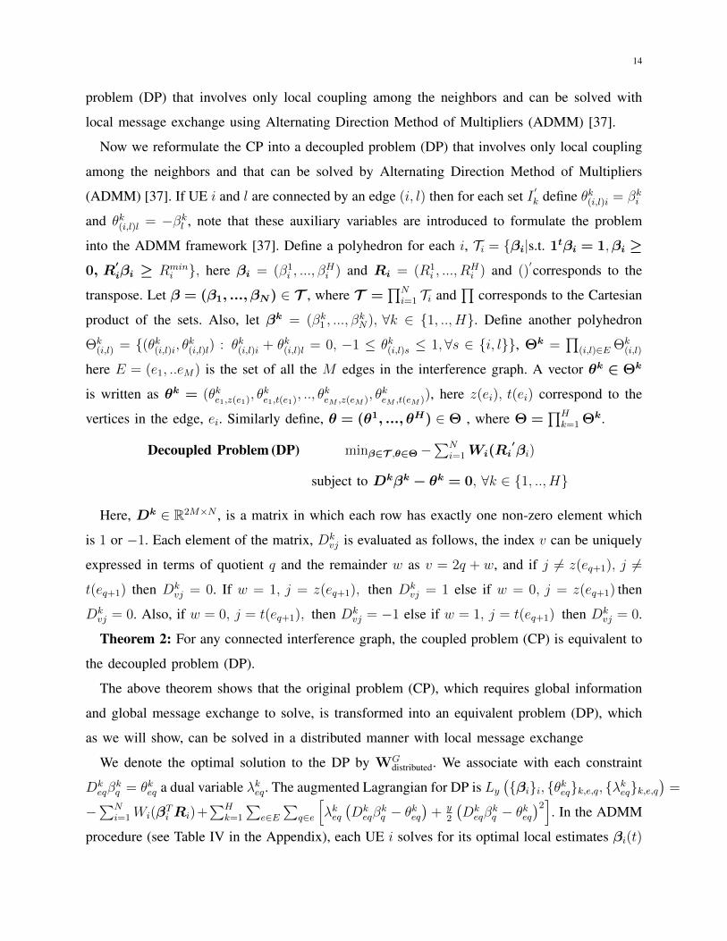
Figure 4. A heterogeneous network of 2 PBS and 2 FBS and their corresponding UEs.

that maximizes the augmented Lagrangian given the previous dual variables λkei(t − 1) and

auxiliary variables θkei(t − 1) . Then it updates its dual variable λkei(t) and auxiliary variable

θkei(t) based on its local estimate βki (t) and its neighbor j’s local estimate βkj (t). This iteration

of updating local estimates, dual variables, and auxiliary variables is repeated P times. Next, it

is shown that this procedure will indeed converge.

Theorem 3: If DP is feasible12, then the ADMM algorithm in Table IV converges to the

optimal value WGdistributed with a rate of convergence O( 1

P).

Step 4. Determining the cycle length and transmission times: At the end of Step 3, all

the UEs have a consensus about the optimal fractions of time allocated to each MIS, namely

β∗i = γ∗ = (γ∗1 , ..., γ∗H), ∀i ∈ {1, .., N}. The MISs transmit in the order of their indices (i.e.,

{1, .., H}) in cycles. In each cycle of transmission, MIS I′

k transmits for⌈

γ∗kmini∈1,...,N γ∗i

× 10d⌉

slots, where we multiply by 10d such that the rounding error is reduced or eliminated in case

that γ∗kmini∈1,...,N γ∗i

is not an integer.

B. A Motivation Example

Consider a network of 2 picocell base stations (PBS) and 2 femtocell base stations (FBS),

each serving one UE. The network topology is shown in Fig. 2. We assume a path loss model

for channel gains, with path loss exponent 4. The maximum transmit power of each UE is 80

mW, and the noise power at each SBS is 1.6× 10−3 mW. UEs in different tiers have different

minimum throughput requirements: FUE (femtocell UE) 1 and FUE 2 in the femtocells require a

minimum throughput 0.4 bits/s/Hz, and PUE (picocell UE) 1 and PUE 2 in the picocells require

0.2 bits/s/Hz. The interference graph is constructed according to a distance based threshold rule

similar to [28]. Specifically, an edge exists between two UE-BS pairs if the distance between

12DP is feasible, if the feasible region resulting from the constraints in DP is non-empty.

16

any pair of SBSs is less than a threshold, which is set to be 1.2m here. There are two MISs.

MIS 1 consists of FUE 1 and FUE 2, and MIS 2 consists of PUE 1 and PUE 2. We consider

two performance criteria: the max-min fairness and the sum throughput. We will compare with

the following state-or-the-art policies:

1. Distributed Constant Power Control Policies [7], [8], [10]: In these policies, all the UEs

choose constant power levels determined by distributed algorithms utilizing information (e.g.,

power levels used by neighbors) made available through local/global message exchange.

2. Optimal Centralized Constant Power Policies: In these policies, all the UEs choose

constant power levels determined by a central controller utilizing global information.

3. Distributed MIS STDMA-1 [6] and STDMA-2 [4]: These policies construct a subset of

the MISs of the interference graph in a distributed manner and propose fixed schedules of the

MISs. Different works adopt different schedules, and we differentiate them by referring to them

as MIS STDMA-1 [6] and STDMA-2 [4].

4. Distributed Joint Power Control and Spatial Reuse [22] [23]: These policies choose one

UE from each cell to form a subset, and schedule these subsets of UEs based on their channel

gains to maximize the sum throughput. The policies are named power matched scheduling (PMS).

In Table 1, we compare the performance of our proposed policy with state-of-the-art policies

for the same setup as in Fig. 1. We compute the optimal centralized constant power control policy

by exhaustive search, which serves as the performance upper bound of the distributed constant

power control policies [7], [8], [10] centralized constant power control policies [15]. In PMS

policies [22] [23], UEs within the same cell are scheduled in a time-division multiple access

(TDMA) fashion, and the active UEs in different cells transmit simultaneously. In this motivating

example, there is one UE in each cell, which will be scheduled to transmit all the time. Therefore,

the PMS policy reduces to a constant power control policy, and is worse than the optimal

centralized constant power control policy. We can see that our proposed policy outperforms

all constant power control policies and distributed PMS policies by at least 375% and 32.8%,

in terms of max-min fairness and sum throughput, respectively. The significant performance

improvement over the constant power control policies results from the elimination of the high

interference among the users through scheduling MISs. Our proposed policy also outperforms

distributed STDMA policies by 30%-40%. As we will see in Section VI, the performance gain is

even higher (160%-700%) in realistic deployment scenarios. Finally, in this motivating example,

17

Table I

COMPARISONS IN TERMS OF MAX-MIN FAIRNESS & SUM THROUGHPUT CRITERION

Policies Max-min Performance Sum Performance

throughput (bits/s/Hz) Gain % throughput (bits/s/Hz) Gain %

Distributed constant power control [7], [8], [10] <0.28 >375 % 6.1 32.8 %

Distributed PMS [22], [23] <0.28 >375% 6.1 32.8 %

Optimal centralized constant power control 0.28 375% 6.1 32.8 %

Distributed MIS STDMA-2/1 [4], [6] 0.96 38.5% 6.25 30.0 %

Proposed (Section-V) 1.33 - 8.12 -

Benchmark Problem (BP) (Section- VI) 1.33 - 8.12 -

the proposed policy achieves the optimal performance of the benchmark problem defined in

Section VI, which is a close approximation of the original problem (CP).

C. Performance Guarantees for Large Networks and Properties of Interference Graphs

In this subsection, we provide performance guarantees for our proposed framework described

in Section V-A. Specifically, we prove that the network performance WGdistributed achieved by the

proposed distributed algorithms has a constant competitive ratio with respect to the optimal value

Wopt of the PDP. Moreover, we prove that the competitive ratio does not depend on the network

size. Our result is strong, because the solution to PDP needs to be computed by a centralized

controller with global information and with NP complexity, while our proposed framework allows

the UEs to compute the policy fast in a distributed manner with local information and local

message exchange.

Before characterizing the competitive ratio analytically, we define some auxiliary variables.

Define the upper and lower bounds on the UEs’ maximum transmit power levels and throughput

requirements as, 0 < pmaxlb ≤ pmaxi ≤ pmaxub ,∀i ∈ {1, ..., N} and, 0 < Rminlb ≤ Rmin

i ≤ Rminub ,∀i ∈

{1, ..., N} respectively. Let Dij is the distance between UE i and SBS j. Define upper and lower

bounds on the distance between any UE and its serving SBS and the noise power at the SBSs

as, 0 < Dlb ≤ DiT (i) ≤ Dub,∀i ∈ {1, ..., N} and, σ2lb ≤ σ2

j ≤ σ2ub, ∀j ∈ {1, ..., K} respectively.

We assume that the channel gain is gij = 1(Dij)np

, where np is the path loss exponent.

Definition 1 (Weak Non-neighboring Interference): The interference graph G exhibits ζ

Weak Non-neighboring Interference (ζ-WNI) if for each UE i the maximum interference from

18

its non-neighbors is bounded, namely∑

j 6∈N (i),j 6=i gjT (i)pmaxj ≤ (2ζ − 1)σ2

ub, ∀i ∈ {1, ..., N}.

Define ∆max =log2(1+

pmaxlb(Dub)np2ζσ2

ub

)

Rminub− 1. Then we have the following theorem for the network

performance criterion, sum throughput13.

Theorem 4: For any connected interference graph, if the maximum degree ∆ ≤ ∆max and it

exhibits ζ-WNI then, our proposed framework of interference management described in Section

V-A achieves a performance WGdistributed ≥ Γ · Wopt with a probability no smaller than (1 −

1Nc1−1 )(1 − 1

Nc2−1 ). Moreover, the competitive ratio Γ =Rminub

log2(1+pmaxub

(Dlb)npσ2lb

)is independent of the

network size.

Note that the analytical expression of competitive ratio, Γ =Rminub

log2(1+pmaxub

(Dlb)npσ2lb

), does not depend

on the size of the network. Our results are derived under the conditions that the interference

graph has a maximum degree bounded by ∆max, and that the interference from non-neighbors

is bounded (i.e. ζ−WNI). These conditions do not restrict the size of the network, next example

illustrates this. In addition, our results hold for any interference graph that satisfy the conditions

in Theorem 4, regardless of how the graph is constructed.

Example: Consider a layout of SBSs in a K ×K square grid, i.e. K2 SBSs with a distance

of 5m between the nearest SBSs. Assume that each UE is located vertically below its SBS at

a distance of 1 m. Fix the parameters pmaxi = 100 mW, σ2i = 3 mW, Rmin

i = 0.1bits/s/Hz,

∀i ∈ {1, .., K2}, np = 4. We construct the interference graph based on the distance rule [28],

namely there is an edge between two pairs if the distance between their SBSs exceeds 6m,

which gives us the maximum degree ∆ = 4. We can also verify that the interference graphs

under any number K2 of SBSs exhibit ζ-WNI with ζ = 0.15 and ∆ < ∆max, where ∆max = 48.

Given ∆ = 4 and ζ = 0.15, from Theorem 4, we get the performance guarantee of 0.17 for

any network size K2. Note that the number 0.17 is a performance guarantee, and that the actual

performance is much higher compared to the performance guarantee as well as those achieved

by state-of-the-art policies (see Section VI).

Both Theorem 1 and 4 required the maximum degree of the interference graph to be bounded

by a given constant. Here, we show that constraint on the degree is natural and is a must to ensure

feasibility, i.e. to satisfy the minimum throughput requirements of every UE. Specifically, we

13We can extend this result for weighted sum throughput, with weights wi = Θ( 1N

), it is not done to avoid complex notations.

19

prove that if the maximum degree exceeds some threshold, then no policy based on scheduling

MISs in ΠMIS (a large space of policies, see Section III) is feasible. Let the construction of

interference graph be based on a distance based threshold rule similar to [28]. An edge exists

between two UE-SBS pairs if and only if, the distance between two SBS is no greater than Dth.

We define the threshold of the maximum degree as ∆∗ (See the Appendix for the expression).

Theorem 5: If the maximum degree of the interference graph ∆ ≥ ∆∗, then any policy based

on scheduling MISs in ΠMIS fails to satisfy the minimum throughput requirements of the UEs.

The intuition behind Theorem 5 is that, if the degree of the interference graph is large then

there must be a large number of UE-SBS pairs which interfere with each other strongly (mutually

connected) which makes it impossible to allocate each UE enough transmission time to satisfy

its minimum throughput requirement.

D. Self-Adjusting Mechanism for Dynamic Entry/Exit of UEs

We now describe how the proposed framework can adjust to dynamic entry/exit by the UEs

in the network without recomputing all the four steps. We allow the UEs to enter and exit, but

number of SBSs is fixed. We only allow let one UE enter or leave the network in any time slot.

1. UE leaves the network: Suppose a UE i which was transmitting to SBS T (i) leaves the

network. If the UE i was transmitting in a set of colors Ci, then as soon as it leaves, these

colors can be potentially used by some neighbors, N (i). The SBS T (i) which was serving the

UE i can have other UEs which are still in the network and transmitting to it. Then for each

color c′ ∈ Ci it first searches among the UEs which it serves that are not already transmitting

in c′ and who also do not have a neighboring UE-SBS pair which is already transmitting in

c′. Let the set of such UEs be UEc′

i,left. SBS T (i) allocates color c′ to the UE whose index is

arg maxj∈UEc′i,leftRc′j . In case UEc′

i,left is empty then that color, c′ is left unused.

2. UE enters the network: Suppose a UE i registered with SBS T (i) enters the network.

i). Given the minimum throughput requirement of the UE i the SBS T (i) first creates a list of

UEs, UEi,enter, which consists of the UEs it is serving and who are transmitting at more than

their minimum throughput requirement.

ii). SBS T (i) creates the list of colors, Ci,enter in which UEs in UEi,enter are transmitting, it

also consists of the colors that are not being used by any UE served by T (i). Next, it creates

valid colors list i.e. Cvalidi,enter from Ci,enter, where a color c ∈ Cvalid

i,enter if c ∈ Ci,enter and if none

of the neighbors of i in N (i) that are not in UEi,enter are already using that color.

20

iii). Next, the SBS T (i) has to allocate some portions from the fractions of time allocated to

the colors in Cvalidi,enter, such that UE-i can transmit and its minimum throughput requirement is

satisfied to the best possible extent. The allocation is done as follows, let Cvalidi,enter = {c′1, ...., c

′s}.

Proceeding sequentially, for each color c′i, SBS T (i) selects the maximum possible portion

to satisfy the minimum throughput requirement of UE-i, such that the minimum throughput

requirements of UEs in UEi,enter, who are using this color, c′i are not violated.

iv). If the requirement of UE-i is not satisfied then, SBS T (i) requests the neighboring UE-

SBSs (apart from the UEs that are served by T (i)) to announce the set of colors which are either

not being used or in which their corresponding UEs are operating at more than the minimum

throughput requirement. From the set of colors that are received, the SBS-T (i) chooses each

color from the list if it is not being used by any other neighboring UE apart from the ones who

sent the announcement. The resulting list of colors is Clvalidi,enter = {c′1, ..., c′

l}.

v). Proceeding sequentially with the colors in Clvalidi,enter, for each color, SBS-T (i) requests a

portion from the fraction of time allocated to that color, to the neighboring UE-SBSs allocated

that color, such that the throughput requirement of UE-i is satisfied. The neighboring UE-SBSs

either allow the requested portion or send the portion which is acceptable to them, i.e. their

throughput requirements are not violated. SBS-T (i) allocates the minimum acceptable portion

to UE-i and proceeds to the next color in the list if the throughput requirements are not satisfied.

E. Extensions

In our model, UEs operate in the same frequency band. However, our methodology can be

extended to scenarios where UEs operate in different frequency channels (frequency reuse) and

transmit at the same time. In this case, the problem is to find the optimal frequency allocation

with the same objective function and constraints as in PDP. To solve this problem, the first two

steps of the framework remain the same. In Step 3, the UEs compute distributedly the optimal

fractions of bandwidth to be allocated to each MIS. This step is equivalent to computing the

optimal fraction of time allocated to each MIS as in our current formulation. In Step 4, the

UEs compute the number of frequency channels allocated to each MIS based on the bandwidth

allocation.

Note that we do not implement beamforming, although beamforming can be used in conjunc-

tion with our policy. If the UEs transmitting to the same SBS cooperate to do beamforming, we

21

can delete the edge between them in the interference graph, and use the new interference graph

in the scenario with beamforming.

VI. ILLUSTRATIVE RESULTS

In this section, we evaluate our proposed policy under a variety of scenarios with different

levels of interference, large numbers of UEs, different performance criteria, time-varying channel

conditions, and dynamic entry and exit of UEs.

We compare our policy with the optimal centralized constant power control policy, the dis-

tributed MIS STDMA-1 [6] and STDMA-2 [4], distributed PMS [22] [23], in terms of sum

throughput and max-min fairness. We do not separately compare with distributed/centralized

constant power control policies in [7], [8], [10] [15], because their performance is upper bounded

by the optimal centralized power control. Since it is difficult to compute the solution to the NP-

hard PDP, we define a benchmark problem, where we restrict our search to policies in which a

UE either transmits at its maximum power level or does not transmit.The space of such policies

can be writtenas ΠBC = {π = (π1, ..., πN) : πi : Z+ → {0, pmaxi } ∀i ∈ {1, .., N}}. The policy

space ΠBC is a subset of all policies Π and is a superset of MIS based policies ΠMIS . In

other words, the benchmark problem has the same objective and constraints as PDP; the only

difference is the policy space to search . Hence, the benchmark problem is a close approximation

of the PDP. Note that the benchmark problem is also NP-hard (see the appendix).

A. Performance under time-varying channel conditions

Consider a 3x3 square grid of 9 SBSs with the minimum distance between any two SBSs

being d = 4.7m. Each SBS serves one UE, who has a maximum power of 1000 mW and a

minimum throughput requirement of 0.45 bits/s/Hz. The UEs and the SBSs are in two parallel

horizontal hyperplanes, and each SBS is vertically above its UE with a distance of√

10m.

Then the distance from UE i to another SBS j is Dij =√

10 + (DBSij )2 , where DBS

ij is the

distance between SBSs i and j. The channel gain from UE i to SBS j is a product of path

loss and Rayleigh fading fij ∼ Rayleigh(β) , namely gij = 1(Dij)2

fij . The density function of

Rayleigh(β) is v(z) = zβ2 e− z2

2β2 for z ≥ 0, and v(z) = 0 for z < 0. The SBSs identify neighbors

using a distance based rule with the threshold distance as in Section V-C with Dth = 7m. Note

that different thresholds lead to different interference graphs, and hence different performance,

which will be discussed next. Although, we use a distance based threshold rule, our framework

22

0.4 0.45 0.5 0.55 0.6 0.65 0.7 0.75 0.8 0.85 0.90.1

0.2

0.3

0.4

0.5

0.6

0.7

0.8

0.9

Fading parameter β

Min

imu

m t

hro

ug

hp

ut

ach

ieve

d b

y a

ny u

se

r (b

its/s

/Hz)

Proposed PolicyOptimal Centralized Constant PowerDistributed MIS STDMA−1Distributed MIS STDMA−2Benchmark Problem

18 % Gap

40 %Increase

Fig. 5 a)

0.4 0.45 0.5 0.55 0.6 0.65 0.7 0.75 0.8 0.85 0.90.1

0.2

0.3

0.4

0.5

0.6

0.7

0.8

0.9

1

1.1

Fading parameter β

Ave

rag

e t

hro

ug

hp

ut

pe

r U

E (

bits/s

/Hz)

Proposed PolicyOptimal Centralized Constant PowerDistributed MIS STDMA−2Benchmark Problem

9 % Gap

88 %Increase

Fig. 5 b)

Figure 5. Comparison of the proposed policy with state of the art under different interference strength and time-varying channel

conditions

is general and does not rely on a particular rule. The resulting interference graph for this setting

is graph 3 shown in Fig. 7 a).

At the beginning, the UE-SBS pairs generate the set of MISs (Step 2 of the design framework

in Section V), and compute the optimal fractions of time allocated to each MIS (Step 3). In

our simulation, we assume a block fading model [38] and the fading changes every 100 time

slots independently. To reduce complexity, the UEs do not recompute the interference graph and

the MISs, but will recompute the optimal fractions of time under the new channel gains every

100 time slots. In Fig. 5, we compare the performance of the proposed policy with state of

the art policies under different variances β of Rayleigh fading. We do not plot the performance

of distributed PMS for this scenario since it is upper bounded by optimal centralized constant

power control (because there is one UE per cell). We do not plot the distributed MIS STDMA -1

either, when the performance criterion is average throughput per UE (i.e., sum throughputN

), because

it cannot satisfy the minimum throughput constraints. From Fig. 5, we can see that in terms of

both average throughput and max-min fairness, our proposed policy achieves large performance

gain (up to 88%) over existing policies, and achieves performance close to the benchmark (as

close as 9%).

Selecting the Optimal Interference Graph : For different values of d, there can be five possible

interference graphs, which are shown in Fig. 7 a). In Fig. 6 a) we show that as the grid size

23

1 2 3 4 5

0.4

0.5

0.6

0.7

0.8

0.9

1

Index of the interference graph

Min

imum

thro

ughp

ut a

chie

ved

by a

ny u

ser

(bits

/s/H

z)

d=4.74 md=3.70 md= 2.52 m

Graph 3 isoptimal for d=4.74m

Graph 2 isoptimal ford=3.70m

Graph 1 isoptimal ford=2.52m

Fig. 6 a)

1 2 3 4 5 6 7 8 9 101

2

3

4

5

6

7

8

9

10

11

Time instance at which number of UEs change

Su

m t

hro

ug

hp

ut

(bits

/s/H

z)

Rmintol

=0.23

Rmintol

=0.25

Rmintol

=0.25

(1,2,2) (1,3,1)(1,3,1)

(1,2,1) (1,2,2)

(0,2,2)

(0,2,2)

(3,3,2) (3,2,2)

(3,2,1) (3,3,1)

(2,3,1)(2,3,0)

(1,3,0)

(0,1,2)

(1,3,1) (1,2,1)

(2,3,1)

(2,3,2)

(2,1,2)

(1,2,1)

(2,1,1)

(1,1,1)

(1,1,1) (1,1,2) (1,2,2)

(0,2,3)

(0,2,2)

(1,1,2)

(a,b,c)−number of UEsin room 1,2 and 3

(1,2,3)

Fig. 6 b)

Figure 6. a) Comparison of max-min fairness under different grid sizes, b) Sample paths of sum throughput under dynamic

entry/exit of UEs in the network

1 2 3 4 5

Fig. 7 a)

Length = 20 m

FBS1 FBS2 FBS3Height

= 2 m

5 m 5 m

Fig. 7 b)

Figure 7. a) Different interference graphs for the 3 x 3 BS grid, b) Illustration of setup with 3 rooms.

d decreases (d = 4.7m, d = 3.7m and d = 2.5m), the levels of interference from the adjacent

UEs increases, and as a result, the interference graph with higher degrees perform better (as d

decreases, the optimal graph changes from graph 3 to graph 1) .

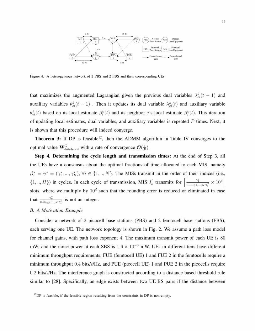
B. Performance scaling in large networks

Consider the uplink of a femtocell network in a building with 12 rooms adjacent to each other.

Fig. 7 b) illustrates 3 of the 12 rooms with 5 UEs in each room. For simplicity, we consider

a 2-dimensional geometry. Each room has a length of 20 meters. In each room, there are P

uniformly spaced UEs, and one SBS installed on the left wall of the room at a height of 2m.

The distance from the left wall to the first UE, as well as the distance between two adjacent UEs

in a room, is 20(1+P )

meters. Based on the path loss model in [39], the channel gain from each

SBS i to a UE j is 1(Dij)2∆nij , where ∆ = 100.25 is the coefficient representing the loss from the

wall, and nij is the number of walls between UE i and SBS j. Each UE has a maximum transmit

power level of 50 mW, a minimum throughput requirement of Rmini = 0.025 bits/s/Hz, and a

24

60 65 70 75 80 85 90 95 100 1050

0.01

0.02

0.03

0.04

0.05

0.06

0.07

0.08

Number of UEs

Min

imum

ave

rage

thro

ughp

ut a

chie

ved

by a

UE

(bi

ts/s

/Hz)

Proposed PolicyDistributed PMSDistributed MIS STDMA−2Distributed MIS STDMA−1

161 %Gain

180 %Gain

Fig. 8 a)

60 65 70 75 80 85 90 95 100 1050

0.1

0.2

0.3

0.4

0.5

0.6

0.7

Number of UEs

Ave

rage

thro

ughp

ut p

er U

E (b

its/s

/Hz)

Proposed PolicyDistributed PMSDistributed MIS STMDA−2Distributed MIS STDMA−1

7 x (times) gain

Fig. 8 b)

Figure 8. Comparison of max-min fairness and average throughput per UE against state of the art for large networks

noise power level of 10−11mW at its receiver. Here, we consider that the UEs use a distance

based threshold rule as in Section V-B with Dth = 30 m. This results in interference graphs

which connects all the UE-SBS pairs within the room and in the adjacent rooms. We vary the

number P of UEs in each room from 5 to 9 and compare the performance in Fig. 8. Note that

the optimal centralized constant power policy cannot satisfy the feasibility conditions for any

number of UEs in each room. Hence, only the performance of distributed MIS STDMA-1,2 and

distributed PMS is shown in Fig. 8. We can see that under both criteria, the performance gain

of our proposed policy is significant (from 160% to 700%). Note that since the number of UEs

is large, it is impossible to solve the benchmark problem (which is NP-hard) is not possible.

C. Self-adjusting mechanism for dynamic entry/exit of the UEs

The self-adjusting mechanism proposed in Section V-D is aimed to provide incoming UEs

with the maximum possible throughput without affecting the incumbent UEs, and to reuse the

time slots left vacant by exiting UEs efficiently. Consider the same setup as in Section VI-B

with 3 rooms and a maximum of P = 3 UEs in each room. Each UE has a maximum transmit

power of 1000 mW and a minimum throughput requirement of 0.25 bits/s/Hz.

We assume that at a given time only one UE either enters or leaves the network. In Fig. 6 b)

we show different sample paths of the sum throughput under different entry and exit processes.

In the legends (i.e., Rmintol), we show the minimum throughput achieved at any point in the

sample path. We repeated the same procedure 100 times. We can see that the self-adjusting

mechanism works well by guaranteeing a worst-case minimum throughput requirement of 0.23

25

bits/s/Hz, which is just 0.02 bits/s/Hz below the original requirement more than 80% of the time.

VII. CONCLUSION

We proposed a design framework for distributed interference management in large-scale,

heterogeneous networks, which are composed of different types of cells (e.g. femtocell, picocell),

have different number of UEs in each cell, and have UEs with different minimum throughput

requirements and channel conditions. Our framework allows each UE to have only local knowl-

edge about the network and communicate only with its interfering neighbors. There are two key

steps in our framework. First, we propose a novel distributed algorithm for the UEs to generate

a set of MISs that span all the UEs. The distributed algorithm for generating MISs requires

O(logN) steps (which is much faster than state-of-the-art) before it converges to the set of

MISs with a high probability. Second, we reformulate the problem of determining the optimal

fractions of time allocated to the MISs in a novel manner such that the optimal solution can be

determined by a distributed algorithm based on ADMM. Importantly, we prove that under wide

range of conditions, the proposed policy can achieve a constant competitive ratio with respect to

the policy design problem which is NP-hard. Moreover, we show that our framework can adjust

to UEs entering or leaving the network. Our simulation results show that the proposed policy

can achieve large performance gains (up to 85%).APPENDIX

Discussion on max-min fairness: We now discuss as to how the proposed framework can be

extended to incorporate inseparable function like max-min fairness. The coupled problem with

max-min fairness objective is restated below:

Coupled Problem (CP) maxα mini∈{1,..,N}

Wi(H∑k=1

αkRki )

subject toH∑k=1

αkRki ≥ Rmin

i , ∀i ∈ {1, ...N}

H∑k=1

αk = 1, αk ≥ 0, ∀k ∈ {1, ..., H}

Transforming the above problem into an equivalent problem with auxiliary variable t is given

as

26

Table II

GENERATING MISS IN A DISTRIBUTED MANNER, ALGORITHM FOR UE i

Phase 1- Initialization: Txitent = φ, Txifinal = φ, tentative and final choice of UE i, RxN (i)tent = φ ,RxN (i)

final = φ tentative

and final choice made by the neighbors, C0i = {1, ..., H} ∩ {1, .., di + 1} the current list of subset of available colors,

Ci = φ, list of colors used by i, Ficolored = φ, C10i = {1, ..., H},the current list of all available colors

for n = 0 to dc1 log 43Ne

Txitent = φ, Txifinal = φ

if(Ficolored = φ)

Txitent = rand{Cni }, rand represents randomly selecting a color and informing the neighbors about it.

RxN (i)tent = {Txktent,∀k ∈ N (i)}

If(Txitent 6= RxN (i)tent (j), ∀j ∈ N (i)), here UE-i checks if there is a conflict with any of the neighbor’s choice

Txifinal = Txitent, Ci = {Txifinal},if there is no conflict then UE-i transmits its final color choice to the neighbors,

else

Txifinal = φ

end

end

RxN (i)final = {Txkfinal,∀k ∈ N (i)}

Cn+1i = Cni ∩ {RxN (i)

final ∪ Txifinal}c, C1n+1i = C1ni ∩ {RxN (i)

final ∪ Txifinal}c

if(Txifinal 6= φ)

Ficolored = 1

end

end

Table III

ADMM UPDATE ALGORITHM FOR UE i

Initialization: arbitrary βi(0) ∈ Bi, θkei(0) such that θk ∈ Θk, and λkei(0) = 0, ∀k ∈ {1, ..., H},∀e such that i ∈ e

For t = 0 to P − 1

βi(t+ 1) = arg minβi∈Bi −∑Ni=1Wi(β

Ti Ri) +

∑Hk=1

∑e∈E

∑q∈e

[λkeq(Dkeqβ

kq − θkeq

)+ y

2

(Dkeqβ

kq − θkeq

)2]βi(t+ 1) is transmitted to all of its neighbors in N (i).

λkei(t) is transmitted to its neighbor connected with edge e, ∀k ∈ {1, ..., H} and ∀e such that i ∈ e

Update ∀k ∈ {1, ..., H} and ∀e such that i ∈ e

λkei(t+ 1) = 12(λkei(t) + λkej(t))− y

2(Dk

eiβki (t+ 1) +Dk

ejβkj (t+ 1)), where j is the other endpoint of e.

θkei(t+ 1) = 1y

(λkei(t+ 1)− λke,i(t)) +Dkeiβ

ki (t+ 1)

end

27

maxα,t t

subject to Wi(H∑k=1

αkRki ) ≥ t, ∀i ∈ {1, ..., N}

H∑k=1

αkRki ≥ Rmin

i , ∀i ∈ {1, ...N}

H∑k=1

αk = 1, αk ≥ 0, ∀k ∈ {1, ..., H}

To decouple the above problem, we introduce local variables for each UE i given as,{β1i , ..., β

H+1i }.

Now we state a problem which we claim is equivalent to CP,(the proof to this claim is very

similar to the proof of Theorem 2 and we will highlight this fact in the proof clearly).

P1 maxβ

N∑i=1

βH+1i

subject to Wi(H∑k=1

βki Rki ) ≥ βH+1

i , ∀i ∈ {1, ..., N}

H∑k=1

βki Rki ≥ Rmin

i , ∀i ∈ {1, ...N}

H∑k=1

βki = 1, βki ≥ 0, ∀k ∈ {1, ..., H},∀i ∈ {1, ..., N}

βki = βkj ,∀j ∈ N (i),∀k ∈ {1, ..., H + 1}

Here, β = (β1, .., βN ), with βi = (β1i , ..., β

H+1i ),∀i ∈ {1, ..., N}. Now, given the two

problems CP and the problem P1 are equivalent, we focus on solving P1. P1 can be changed

to a problem similar to DP. To do that we introduce some additional variables similar to

the ones introduced for DP. If UE i and l are connected by an edge (i, l) then for each set

I′

k define θk(i,l)i = βki and θk(i,l)l = −βkl , note that these auxiliary variables are introduced

to formulate the problem into the ADMM framework [37]. Define a polyhedron for each i,

T ′i = {(β1)i|s.t. 1t(β′′

i ) = 1, (β1)i ≥ 0, R′

i(β′′

i ) ≥ Rmini ,Wi(R

′

i(β′′

i )) − βH+1i ≥ 0},

here β′′

i = (β1i , ..., β

Hi ) and Ri = (R1

i , ..., RHi ) and ()

′corresponds to the transpose. Let β =

(β1, ..., βN) ∈ T ′ , where T ′=∏N

i=1 T′i and

∏corresponds to the Cartesian product of

28

the sets. Also, let βk = (βk1 , ..., βkN), ∀k ∈ {1, .., H}. Define another polyhedron Θk

(i,l) =

{(θk(i,l)i, θk(i,l)l) : θk(i,l)i + θk(i,l)l = 0, −1 ≤ θk(i,l)s ≤ 1,∀s ∈ {i, l}}, Θk =∏

(i,l)∈E Θk(i,l) here

E = (e1, ..eM) is the set of all the M edges in the interference graph. A vector θk ∈ Θk

is written as θk = (θke1,z(e1), θke1,t(e1), .., θ

keM ,z(eM ), θ

keM ,t(eM )), here z(ei), t(ei) correspond to the

vertices in the edge, ei. Similarly define, θ = (θ1, ..., θH+1) ∈ Θ′ , where Θ

′=∏H+1

k=1 Θk.

The reformulated problem is stated as follows:

DP1 minβ∈T ′ ,θ∈Θ′ −∑N

i=1Wi(Ri′βi)

subject to Dkβk − θk = 0, ∀k ∈ {1, .., H + 1}

Then, DP1 can be solved using the ADMM procedure similar to the one described for DP.

Discussion on Benchmark Problem’s complexity: Benchmark Problem is restated here for

convenience:

Benchmark Problem (BP) maxπ∈ΠBC

W (R1(π), ..., RN(π))

subject to. Ri(π) ≥ Rmini , ∀i ∈ {1, ..., N}

Let the power set of U be SU , where SU consists of 2N subsets of UEs. Let SU(j) denote the

jth element of SU . Define a set of power profiles,PSU , where the PSU (j) corresponds to the jth

element in the set and it corresponds to the power profile when the UEs in set SU(j) transmit at

their maximum power levels and the rest of the UEs do not transmit. Note that for π ∈ ΠBC ,

π(t) corresponds to a power profile in PSU . Therefore, the average throughput achieved by

UE i, Ri(π), where π ∈ ΠBC , can also be expressed as Ri(π) =∑2N

j=1 αjri(PSU (j)), with

αj ≥ 0,∀j ∈ {1, .., 2N}and∑2N

j=1 αj = 1. Here the fraction αj associated with each profile

PSU (j) corresponds to the fraction of transmission time associated with that power profile.

29

Consider the following problem:

BP1 maxy,α

W (y1, ..., yN)

subject to. yi ≥ Rmini , ∀i ∈ {1, ..., N}

yi =2N∑i=1

αiri(PSU (j)), ∀i ∈ {1, ..., N}

αj ≥ 0,∀j ∈ {1, .., 2N},2N∑j=1

αj = 1

Next, in order to show that the above problem is NP-hard we will show intuitively why is it

so, but the detailed proof follows from proof of Theorem 1 in [40]. Consider W (y1, .., yN) =∑Ni=1 yi ,to be a linear function, Rmin

i = 0, ∀i ∈ {1, ..., N} and the cross channel gains amongst

some users who do not share an edge in the interference graph to be 0 and the cross channel

gains amongst the interfering neighbors to be ∞. This implies that in any optimal solution

will correspond to the transmission by a MIS of the interference graph. This can be justified as

follows. Consider an optimal solution in which two neighboring UEs are transmitting, making one

of the UEs not transmit will definitely increase the sum throughput contradicting the optimality.

Specifically, this problem reduces to finding the maximum weighted maximum indpendenet set

which is NP hard. Here the weight of each MIS corresponds to∑N

i=1 ri(pIj ).

Proof of Theorem 1: The success probability of Phase 1 is high, (1− 1Nc1−1 ) (lower bound),

(see [35] for detail), here we analyze Phase 2.

We first show that, if the list of remaining colors given as, C1ni is empty at n ≥ dc1 log 43Ne+

dc2 logxNe + 2 and if this holds ∀i ∈ {1, ..., N} then the Phase 2 has converged to a set of

H MISs which span all the UEs. Let us assume otherwise, i.e. C1ni is empty ∀i ∈ {1, ..., N}

however, the set corresponding to some color h ∈ {1, ..., H}, I ′h is not a MIS. I ′h has to be an

IS. Assume otherwise, i.e. I ′h is not an IS, which implies that there must exist a pair of UEs,

i and j, which are neighbors and are a part of I ′h. If this is true then both then both acquired

the color h either in the same time slot or in different time slots, in Phase 1 or 2. In case the

color is acquired in different time slots, then after the first time slot when either of the UEs in

the pair acquires the color it will transmit the final color choice, h to the neighbors (see Table

II and III) who in turn delete that color. However, if the color is deleted by the neighbor then

it cannot acquire it in the future thus, ruling out the case that the colors were acquired in two

30

different time slots. If the color was acquired by the UEs in the same time slot, then it implies

that despite the conflict in tentative choice the UEs acquire the color which is not possible (see

Table II and III). This shows that I ′h is an IS.

Since I ′h is not maximal then ∃ at least one UE-j 6∈ I ′k which can be added to this set without

violating independence. From the assumption, we have C1nj = φ which implies that the color

h was deleted at some stage from the original list of all the colors either in Phase 1 or 2. The

deletion of h was a result of that color being acquired finally by at least one of the neighbors

k ∈ N (j) since j 6∈ I′

k. In that case, j cannot acquire h as it will violate the independence

property.

Next, we show that indeed the list of all colors available C1ni is empty at the end of Phase 2

with a high probability. Let Un correspond to the number of UEs which have a non-empty list

at the beginning of time slot n and, let Tn(Un) correspond to the total time needed before all

the UEs have an empty list. The probability that a UE at time slot n with a non-empty list will

have an empty list in next time slot is always greater than cH(1− c)H2 . This can be explained

as, if the UE chooses all the colors in the list assuming (worst case H number of colors remain)

and all the neighbors (worst case H neighbors) do not choose any color, then all the colors

in the UE’s list will be deleted. From this, we get E(Un+1) ≤ (1 − cH(1 − c)H2)Un = 1

xUn

and Tn(Un) = 1 + Tn(Un+1). Assuming that the Phase 2 will start with N UEs whose list

are non-empty (worst case) and from [41] we get P (Tn(N) ≥ dc2 logxNe) ≤ 1Nc2−1 . This

gives the lower bound on success probability of Phase 2 and thereby the result in the Theorem.

(Q.E.D)

Proof of Theorem 2: The two problems which are introduced to transit from CP to DP are,

Global Primal Problem (GPP) max{βki }i,k∑H

k=1Wi(∑N

i=1 βki R

ki )

subject to∑H

k=1 βki R

ki ≥ Rmin

i ,∑H

k=1 βki = 1, ∀i ∈ {1, ..., N}

βki = βkl , ∀i 6= l,∀k ∈ {1, ..., H}, βki ≥ 0, ∀i ∈ {1, ..., N},∀k ∈ {1, ...H}

The second problem, Local Primal Problem (LPP) is the same as GPP except we choose a

subset of the constraints from the above problem. Basically, instead of an equality constraint

between the UE’s estimate and every other UE in the network, we only keep the equality

constraints between the UE and its neighbors, i.e. βki = βkl , ∀k ∈ {1, ..., H},∀l ∈ N (i). This is

formally stated below:

31

Local Primal Problem (LPP) max{βki }i,k∑H

k=1Wi(∑N

i=1 βki R

ki )

subject to∑H

k=1 βki R

ki ≥ Rmin

i ,∑H

k=1 βki = 1, ∀i ∈ {1, ..., N}

βki = βkl , ∀l 6∈ N (i),∀k ∈ {1, ..., H}, βki ≥ 0, ∀i ∈ {1, ..., N},∀k ∈ {1, ...H}

To show that problems CP and GPP are equivalent, we need to show that from β∗ =

(β∗1, .., β∗N ), an optimal argument of GPP, we can obtain an optimal argument of CP, i.e. α∗

and vice versa. Since β∗ is the optimal value (assuming feasibility) we know that β∗i = β∗j

(component-wise) holds ∀i, j ∈ {1, ..., N}.

a).Let α′= β∗i . α′ satisfies the constraints in CP. The objective of CP at α′ attains the optimal

value of GPP. We need to establish that α′ is indeed the optimal argument of CP. Assume that

α′is not the optimal value, then there exists another α∗ which is indeed the optimal. Next, using

α∗, we can obtain another β′as follows, β′1 = α∗and β′

i = β′1, ∀i ∈ {1, ..., N}. The objective

of GPP at β′ should be higher than β∗ which contradicts β∗ being the optimal argument. Note

that if either of CP or GPP is infeasible then the other problem can be shown to be infeasible

as well. On the same lines we can show that from an α∗ we can obtain β∗ as well.

b). Let α∗ be the optimal solution to CP, and define β′′a solution to GPP as follows. Let

β′′1 = α∗ and β′′

i = β′′

j , ∀j 6= i and since α∗ satisfies the constraints of CP, i.e. it is feasible,

implies that β′′ as well satisfies constraints of GPP. We want to show that β′′is the optimal value

as well, assume that it is not and there exists an argument β∗ for which the objective takes a

higher value. If this is the case then, from β∗ we can construct a α′as in part a). which, if β∗

takes a higher value than β′′ , takes a higher value than α∗ thus, contradicting optimality.

To show that GPP and LPP are equivalent, we use the following fact, since LPP consists of a

subset of the constraints then the solution of LPP is an upper bound of the solution to GPP. We

need to show that the gap between the solution of LPP and GPP is always 0. Note that for an

optimal solution of LPP, γ∗ = (γ∗1 , .., γ∗N) we know that γ∗i = γ∗j ∀j ∈ N (i) (component-wise).

If we can show that γ∗i = γ∗j ∀j ∈ {1, ..., N} then LPP and GPP will be equivalent, since it

will also satisfy all the constraints of GPP. Assume that this does not hold then ∃ i, j such that

γ∗i 6= γ∗j . Since, the interference graph is connected ∃ a path i→ j = {i1, ..., is} which implies,

γ∗i = γ∗i1 ... = γ∗j . This leads to a contradiction, thereby establishing the claim.

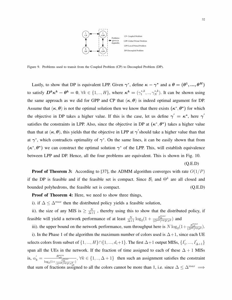
32

1.

CP

2.

GPP

3.

LPP

4.

DP

Problems

given in

Appendix

CP- Coupled Problem

GPP-Global Primal Problem

LPP-Local Primal Problem

DP-Decoupled Problem

Figure 9. Problems used to transit from the Coupled Problem (CP) to Decoupled Problem (DP).

Lastly, to show that DP is equivalent LPP. Given γ∗, define κ = γ∗ and a θ = (θ1, ..., θH)

to satisfy Dkκk − θk = 0, ∀k ∈ {1, .., H}, where κk = (γ∗,k1 , .., γ∗,kN ). It can be shown using

the same approach as we did for GPP and CP that (κ,θ) is indeed optimal argument for DP.

Assume that (κ,θ) is not the optimal solution then we know that there exists (κ∗,θ∗) for which

the objective in DP takes a higher value. If this is the case, let us define γ′= κ∗, here γ′

satisfies the constraints in LPP. Also, since the objective in DP at (κ∗,θ∗) takes a higher value

than that at (κ,θ), this yields that the objective in LPP at γ′should take a higher value than that

at γ∗, which contradicts optimality of γ∗. On the same lines, it can be easily shown that from

(κ∗,θ∗) we can construct the optimal solution γ∗ of the LPP. This, will establish equivalence

between LPP and DP. Hence, all the four problems are equivalent. This is shown in Fig. 10.

(Q.E.D)

Proof of Theorem 3: According to [37], the ADMM algorithm converges with rate O(1/P )

if the DP is feasible and if the feasible set is compact. Since Bi and Θk are all closed and

bounded polyhedrons, the feasible set is compact. (Q.E.D)

Proof of Theorem 4: Here, we need to show three things,

i). if ∆ ≤ ∆max then the distributed policy yields a feasible solution,

ii). the size of any MIS is ≥ N∆+1

, thereby using this to show that the distributed policy, if

feasible will yield a network performance of at least N∆+1

log2(1 +pmaxlb

(Dub)np2ζσ2 ) and

iii). the upper bound on the network performance, sum throughput here is N log2(1+pmaxub

(Dlb)npσ2 ).

i). In the Phase 1 of the algorithm the maximum number of colors used is ∆+1, since each UE

selects colors from subset of {1, ..., H}∩{1, ..., di+1}. The first ∆+1 output MISs, {I ′1, ..., I′∆+1}

span all the UEs in the network. If the fraction of time assigned to each of these ∆ + 1 MISs

is, α′k =Rminub

log2(1+pmaxlb

(Dub)np2ζσ2ub

), ∀k ∈ {1, ..,∆ + 1} then such an assignment satisfies the constraint

that sum of fractions assigned to all the colors cannot be more than 1, i.e. since ∆ ≤ ∆max =⇒

33

(∆ + 1)Rminub

log2(1+pmaxlb

(Dub)np2ζσ2)≤ 1. Using the fact that network exhibits ζ−WNI we can write the

minimum instantaneous throughput that can be obtained by UE-i as, log2(1+pmaxi

(DiT (i))np2ζσ2

ub), and

minimum instantaneous throughput of any UE as, log2(1+pmaxlb

(Dub)np2ζσ2ub

). Thus, given the fractions

assigned to the MISs, α′k =Rminub

log2(1+pmaxlb

(Dub)np2ζσ2ub

), ∀k ∈ {1, ..,∆+1}, which span all the UEs. each

UE i’s throughput requirement is satisfied, , Rminub

log2(1+pmaxlb

(Dub)np2ζσ2ub

)log2(1 +

pmaxi

(DiT (i))np2ζσ2

ub) ≥ Rmin

ub .

ii). Assume that ∃ an MIS whose size is S < N∆+1

. Each UE in the MIS can exclude a

maximum of ∆ UEs from being included in the MIS. This implies that S(∆ + 1), represents the

total number of UEs excluded and the UEs in the MIS which put together should exceed N . Since

this is not the case here, the contradiction implies that S ≥ N∆+1

. This combined with minimum

instantaneous throughput of any UE, we get the lower bound N∆+1

log2(1 +pmaxlb

(Dub)np2ζσ2ub

),for our

policy.

iii). The upper bound on the optimal network performance is obtained by summing maximum

instantaneous throughput of any UE log2(1 +pmaxub

(Dlb)npσ2lb

) for all UEs, N log2(1 +pmaxub

(Dlb)npσ2lb

).

Computing the ratio of the lower bound of proposed scheme N∆+1

log2(1 +pmaxlb

(Dub)np2ζσ2 ) and

N log2(1 +pmaxub

(Dlb)npσ2 ), we getlog2(1+

pmaxlb(Dub)np2ζσ2

)

(∆+1) log2(1+pmaxub

(Dlb)npσ2)

which is no less than, Γ =Rminub

log2(1+pmaxub

(Dlb)npσ2)

since ∆ ≤ ∆max. (Q.E.D)

Proof of Theorem 5: Let ∆∗ = 6η with η = dlog2(1+ 1

(Dlb)npσ2lb

pmaxub )

Rminlbe. We assume that the

interference graph is constructed using a distance threshold rule (Subsection V-B). Note that

each UE’s minimum throughput requirement is at least Rminlb , this combined with maximum

instantaneous throughput of any UE log2(1 +pmaxub

(Dlb)npσ2lb

) yields that each UE needs at leastRminlb

log2(1+pmaxub

(Dlb)npσ2lb

)fraction of time slots. First, we need to show that if there exists a clique (a

subset of vertices in the graph which are mutually connected) in the interference graph of size,

X greater than η then the minimum throughput constraints cannot be satisfied. Assume that

there does exist such a clique, then any MIS based scheduling policy will allocate separate time

slots to each UE in the clique. This is true because no two UEs in the clique will belong to the

same MIS. This implies that X Rminlb

log2(1+pmaxub

(Dlb)npσ2lb

)is the total fraction separate time slots needed

which has to be less than 1. But as X ≥ η, this leads to infeasibility. Next, if ∆ ≥∆∗, we claim

that we will have at least one clique in the graph satisfying this condition. Then ∃ UE-i with a

degree di ≥ 6η, this implies that within a radius of Dth around SBS-T (i) ∃ 6η SBSs. Also, this

34

circle around SBS-T (i) can be partitioned into 6 sectors subtending π3

at the center.The distance

between any two points located in the sector is ≤ Dth, which we justify next. Hence, all the

points in a sector are mutually connected, thus forming a clique.

Let the 2-D polar coordinates of two points i, j in a sector be (ri, 0) and (rj, θ), where

0 ≤ ri ≤ Dth, 0 ≤ rj ≤ Dth and 0 ≤ θ ≤ π3. Hence, the square of the distance between the two

points is expressed as f(ri, rj, θ) = r2i +r2

j −2rirjcosθ and our claim is that the maximum value

f(ri, rj, θ), in the set of constraints above is no greater than (Dth)2. We formally state this as

an optimization problem below:

maxri,rj ,θ

f(ri, rj, θ)

0 ≤ ri ≤ Dth, 0 ≤ rj ≤ Dth

0 ≤ θ ≤ π3

Since, both ri, rj are non-negative, this implies that in the above optimization problem, θ = π3

has to be satisfied in the optimal argument. Substituting θ = π3

in f(ri, rj, θ) we get, f(ri, rj,π3) =

r2i + r2

j − rirj . Next, we show that r2i + r2

j − rirj ≤ (Dth)2 for 0 ≤ ri ≤ Dth, 0 ≤ rj ≤ Dth.

Fix a 0 ≤ rj ≤ Dth,then r2i + r2

j − rirj takes its maximum value at ri = Dth, which gives

(Dth)2 + r2j − Dthrj . Since 0 ≤ rj ≤ Dth, this yields (Dth)2 + r2

j − Dthrj ≤ (Dth)2 which

establishes the claim.

If we have a total of 6η SBSs in the circle then at least one sector has to have more than η

SBSs (Pigeonhole principle), which implies that a clique of size X ≥ η will exist. (Q.E.D)

REFERENCES

[1] E. Hossain, L. B. Le, and D. Niyato, “Self-organizing small cell networks,” in Radio Resource Management in Multi-Tier

Cellular Wireless Networks. Hoboken, NJ, USA: John Wiley Sons, Inc., 2013.

[2] A. Ghosh, N. Mangalvedhe, R. Ratasuk, B. Mondal, M. Cudak, E. Visotsky, T. A. Thomas, J. G. Andrews, P. Xia, H. S.

Jo et al., “Heterogeneous cellular networks: From theory to practice,” Communications Magazine, IEEE, vol. 50, no. 6,

pp. 54–64, 2012.

[3] J. G. Andrews, H. Claussen, M. Dohler, S. Rangan, and M. C. Reed, “Femtocells: Past, present, and future,” Selected

Areas in Communications, IEEE Journal on, vol. 30, no. 3, pp. 497–508, 2012.

[4] R. Ramaswami and K. K. Parhi, “Distributed scheduling of broadcasts in a radio network,” in INFOCOM’89. Proceedings

of the Eighth Annual Joint Conference of the IEEE Computer and Communications Societies. Technology: Emerging or

Converging, IEEE. IEEE, 1989, pp. 497–504.

[5] I. Cidon and M. Sidi, “Distributed assignment algorithms for multihop packet radio networks,” Computers, IEEE

Transactions on, vol. 38, no. 10, pp. 1353–1361, 1989.

35

[6] A. Ephremides and T. V. Truong, “Scheduling broadcasts in multihop radio networks,” Communications, IEEE Transactions

on, vol. 38, no. 4, pp. 456–460, 1990.

[7] J. Huang, R. A. Berry, and M. L. Honig, “Distributed interference compensation for wireless networks,” Selected Areas

in Communications, IEEE Journal on, vol. 24, no. 5, pp. 1074–1084, 2006.

[8] C. U. Saraydar, N. B. Mandayam, and D. Goodman, “Pricing and power control in a multicell wireless data network,”

Selected Areas in Communications, IEEE Journal on, vol. 19, no. 10, pp. 1883–1892, 2001.

[9] ——, “Efficient power control via pricing in wireless data networks,” Communications, IEEE Transactions on, vol. 50,

no. 2, pp. 291–303, 2002.

[10] E. J. Hong, S. Y. Yun, and D.-H. Cho, “Decentralized power control scheme in femtocell networks: A game theoretic

approach,” in Personal, Indoor and Mobile Radio Communications, 2009 IEEE 20th International Symposium on, Sept

2009, pp. 415–419.

[11] L. Giupponi and C. Ibars, “Distributed interference control in ofdma-based femtocells,” in Personal Indoor and Mobile

Radio Communications (PIMRC), 2010 IEEE 21st International Symposium on. IEEE, 2010, pp. 1201–1206.

[12] A. Ladanyi, D. Lopez-Perez, A. Juttner, X. Chu, and J. Zhang, “Distributed resource allocation for femtocell interference

coordination via power minimisation,” in GLOBECOM Workshops (GC Wkshps), 2011 IEEE, Dec 2011, pp. 744–749.

[13] H.-S. Jo, C. Mun, J. Moon, and J.-G. Yook, “Interference mitigation using uplink power control for two-tier femtocell

networks,” Wireless Communications, IEEE Transactions on, vol. 8, no. 10, pp. 4906–4910, 2009.

[14] M. Bennis, S. M. Perlaza, P. Blasco, Z. Han, and H. V. Poor, “Self-organization in small cell networks: A reinforcement

learning approach,” Wireless Communications, IEEE Transactions on, vol. 12, no. 7, pp. 3202–3212, 2013.

[15] M. Chiang, C. W. Tan, D. P. Palomar, D. O’Neill, and D. Julian, “Power control by geometric programming,” Wireless

Communications, IEEE Transactions on, vol. 6, no. 7, pp. 2640–2651, 2007.

[16] A. Gjendemsj, D. Gesbert, G. E. Oien, and S. G. Kiani, “Binary power control for sum rate maximization over multiple

interfering links,” Wireless Communications, IEEE Transactions on, vol. 7, no. 8, pp. 3164–3173, 2008.

[17] S. Stanczak, M. Wiczanowski, and H. Boche, Fundamentals of resource allocation in wireless networks: theory and

algorithms. Springer, 2009, vol. 3.

[18] J. Ling, D. Chizhik, and R. Valenzuela, “On resource allocation in dense femto-deployments,” in Microwaves, Communi-

cations, Antennas and Electronics Systems, 2009. COMCAS 2009. IEEE International Conference on. IEEE, 2009, pp.

1–6.

[19] G. J. Foschini and Z. Miljanic, “A simple distributed autonomous power control algorithm and its convergence,” Vehicular

Technology, IEEE Transactions on, vol. 42, no. 4, pp. 641–646, 1993.

[20] S. G. Kiani and D. Gesbert, “Maximizing the capacity of large wireless networks: optimal and distributed solutions,” in

Information Theory, 2006 IEEE International Symposium on. IEEE, 2006, pp. 2501–2505.

[21] S. G. Kiani, G. E. Oien, and D. Gesbert, “Maximizing multicell capacity using distributed power allocation and scheduling,”

in Wireless Communications and Networking Conference, 2007. WCNC 2007. IEEE. IEEE, 2007, pp. 1690–1694.

[22] S. G. Kiani and D. Gesbert, “Optimal and distributed scheduling for multicell capacity maximization,” Wireless

Communications, IEEE Transactions on, vol. 7, no. 1, pp. 288–297, 2008.

[23] D. Gesbert, S. G. Kiani, A. Gjendemsjo et al., “Adaptation, coordination, and distributed resource allocation in interference-

limited wireless networks,” Proceedings of the IEEE, vol. 95, no. 12, pp. 2393–2409, 2007.

[24] C.-C. Chen and D.-S. Lee, “A joint design of distributed qos scheduling and power control for wireless networks.” in

INFOCOM, 2006.

36

[25] V. Chandrasekhar, J. G. Andrews, T. Muharemovict, Z. Shen, and A. Gatherer, “Power control in two-tier femtocell

networks,” Wireless Communications, IEEE Transactions on, vol. 8, no. 8, pp. 4316–4328, 2009.

[26] R. Etkin, A. Parekh, and D. Tse, “Spectrum sharing for unlicensed bands,” Selected Areas in Communications, IEEE

Journal on, vol. 25, no. 3, pp. 517–528, 2007.

[27] Y. Wu, B. Wang, K. R. Liu, and T. C. Clancy, “Repeated open spectrum sharing game with cheat-proof strategies,” Wireless

Communications, IEEE Transactions on, vol. 8, no. 4, pp. 1922–1933, 2009.

[28] K. Jain, J. Padhye, V. N. Padmanabhan, and L. Qiu, “Impact of interference on multi-hop wireless network performance,”

Wireless networks, vol. 11, no. 4, pp. 471–487, 2005.

[29] H. Li, X. Xu, D. Hu, X. Qu, X. Tao, and P. Zhang, “Graph method based clustering strategy for femtocell interference

management and spectrum efficiency improvement,” in Wireless Communications Networking and Mobile Computing

(WiCOM), 2010 6th International Conference on. IEEE, 2010, pp. 1–5.

[30] S. Uygungelen, G. Auer, and Z. Bharucha, “Graph-based dynamic frequency reuse in femtocell networks,” in Vehicular

Technology Conference (VTC Spring), 2011 IEEE 73rd. IEEE, 2011, pp. 1–6.

[31] P. Lee, T. Lee, J. Jeong, and J. Shin, “Interference management in lte femtocell systems using fractional frequency reuse,”

in Advanced Communication Technology (ICACT), 2010 The 12th International Conference on, vol. 2. IEEE, 2010, pp.

1047–1051.

[32] C. W. Tan, S. Friedland, and S. H. Low, “Spectrum management in multiuser cognitive wireless networks: Optimality and

algorithm,” Selected Areas in Communications, IEEE Journal on, vol. 29, no. 2, pp. 421–430, 2011.

[33] K. Han, S. Woo, D. Kang, and S. Choi, “Automatic neighboring bs list generation scheme for femtocell network,” in

Ubiquitous and Future Networks (ICUFN), 2010 Second International Conference on. IEEE, 2010, pp. 251–255.

[34] D. Lopez-Perez, I. Guvenc, G. De La Roche, M. Kountouris, T. Q. Quek, and J. Zhang, “Enhanced intercell interference

coordination challenges in heterogeneous networks,” Wireless Communications, IEEE, vol. 18, no. 3, pp. 22–30, 2011.

[35] Ö. Johansson, “Simple distributed ∆ + 1 coloring of graphs,” Information Processing Letters, vol. 70, no. 5, pp. 229–232,

1999.

[36] D. P. Bertsekas and J. N. Tsitsiklis, Parallel and distributed computation: numerical methods. Prentice-Hall, Inc., 1989.

[37] E. Wei and A. Ozdaglar, “On the o (1/k) convergence of asynchronous distributed alternating direction method of

multipliers,” arXiv preprint arXiv:1307.8254, 2013.

[38] A. Goldsmith, Wireless communications. Cambridge university press, 2005.

[39] S. Y. Seidel and T. S. Rappaport, “914 mhz path loss prediction models for indoor wireless communications in multifloored

buildings,” Antennas and Propagation, IEEE Transactions on, vol. 40, no. 2, pp. 207–217, 1992.

[40] Z.-Q. Luo and S. Zhang, “Dynamic spectrum management: Complexity and duality,” Selected Topics in Signal Processing,

IEEE Journal of, vol. 2, no. 1, pp. 57–73, 2008.

[41] R. M. Karp, “Probabilistic recurrence relations,” Journal of the ACM (JACM), vol. 41, no. 6, pp. 1136–1150, 1994.