ke 2 - management accounting information … ke 2 - management accounting information suggested...

1

KE 2 - MANAGEMENT ACCOUNTING INFORMATION

Suggested Answers and Marking Grid

Suggested Answers and Marking Grid

2

SECTION 1

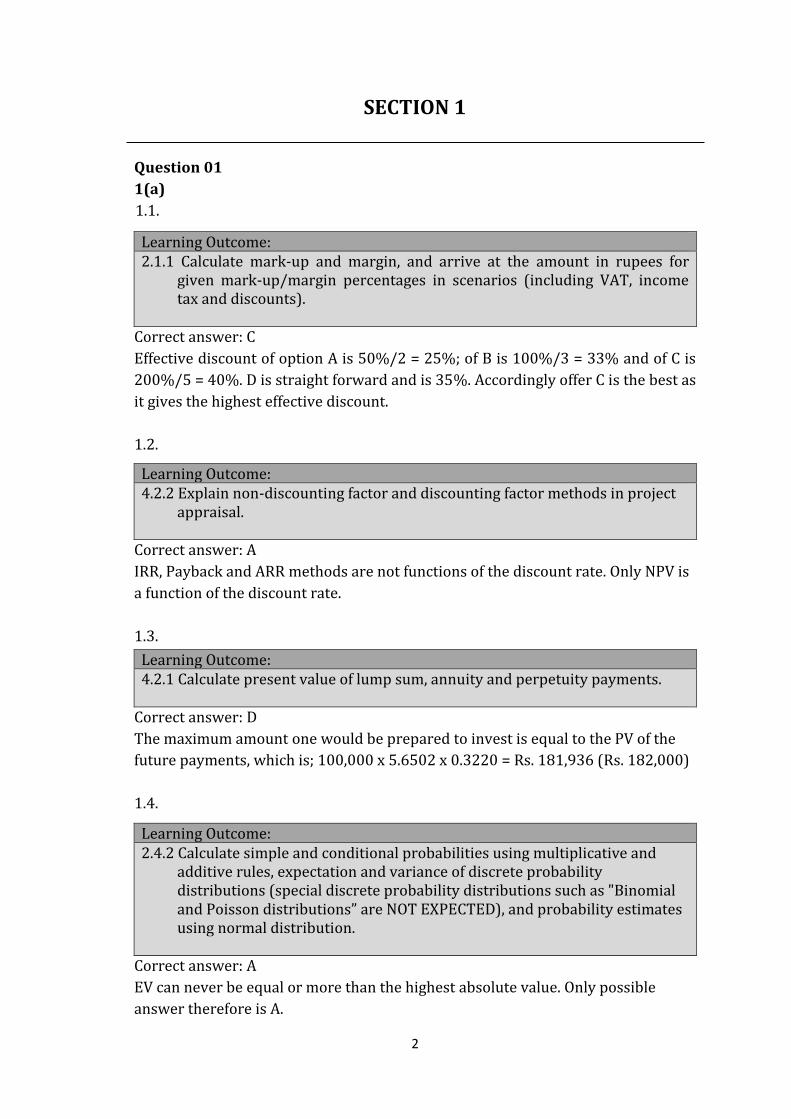
Question 01

1(a)

1.1.

Correct answer: C

Effective discount of option A is 50%/2 = 25%; of B is 100%/3 = 33% and of C is

200%/5 = 40%. D is straight forward and is 35%. Accordingly offer C is the best as

it gives the highest effective discount.

1.2.

Correct answer: A

IRR, Payback and ARR methods are not functions of the discount rate. Only NPV is

a function of the discount rate.

1.3.

Correct answer: D

The maximum amount one would be prepared to invest is equal to the PV of the

future payments, which is; 100,000 x 5.6502 x 0.3220 = Rs. 181,936 (Rs. 182,000)

1.4.

Correct answer: A

EV can never be equal or more than the highest absolute value. Only possible

answer therefore is A.

Learning Outcome: 2.1.1 Calculate mark-up and margin, and arrive at the amount in rupees for

given mark-up/margin percentages in scenarios (including VAT, income tax and discounts).

Learning Outcome: 4.2.2 Explain non-discounting factor and discounting factor methods in project

appraisal.

Learning Outcome: 4.2.1 Calculate present value of lump sum, annuity and perpetuity payments.

Learning Outcome: 2.4.2 Calculate simple and conditional probabilities using multiplicative and

additive rules, expectation and variance of discrete probability distributions (special discrete probability distributions such as "Binomial and Poisson distributions” are NOT EXPECTED), and probability estimates using normal distribution.

3

1.5.

Correct answer: A

Bigger the coefficient of variation (COV = SD/Mean) wider the spread; COV of each

of the data sets are (A) 0.167; (B) 0.114; (C) 0.125; (D) 0.120 and the biggest is

that of A.

1.6.

Correct answer: B

In EOQ model there is no requirement for the lead time to be zero; But all other

assumptions are required.

1.7.

Correct answer: B

Closing inventory under AC is always higher due to absorption of FOH thus option

A and D are not correct. Since inventory has increased, FOH c/f through inventory

is greater than what is getting charged from b/f inventory thus AC profit will be

higher; hence option B is correct.

1.8.

Correct answer: D

In option D there is no reduction in consumption of RM per unit compared to the

standard. But in options A, B and C there could be such a reduction.

Learning Outcome: 2.3.1 Calculate and interpret mean, standard deviation and coefficient of

variation.

Learning Outcome: 1.2.2 Explain material control systems and calculate EOQ, reorder levels,

maximum and minimum levels, valuation of stocks and the issues using FIFO, LIFO and AVCO and calculate profit under each stock valuation method.

Learning Outcome: 3.1.1 Explain the steps involved in absorption costing and marginal costing, and

their relevance in the modern business environment.

Learning Outcome: 5.2.1 Calculate and interpret basic variances on direct material cost, direct

labour cost, variable production overheads, fixed production overheads, and sales.

4

1.9.

Correct answer: C

Std Error is SD(100) / SqRt of sample size(10) = 10; Z@95% is approx 2; Hence

UCL is 600 + 2x10 = 620

1.10.

Correct answer: A

Standard error of proportion = SqRt of (0.2 x 0.8 / 100) = 0.04 = 4%;

Interval @ 95% Confidence = 20% +/- 2 x 4% = 12% to 28%

1(b)

1.11

9 years

Workings ('000)

1800 = 100 + 125 + 150 + …………n years

= n/2 {2x100 + (n-1)x25}

25n2 + 175n – 3600 = 0;

n2 + 7n – 144 = 0;

(n + 16)(n – 9) = 0

n = 9

Learning Outcome: 5.2.1 Calculate and interpret basic variances on direct material cost, direct

labour cost, variable production overheads, fixed production overheads, and sales.

Learning Outcome: 2.5.1 Demonstrate a basic understanding of sampling (simple random sampling

and large samples only), sampling distributions of sample mean and sample proportions, and use of confidence intervals in business including their interpretation.

Marking Guide Each question carries 2 marks. Total 20 marks.

Learning Outcome 7.2.1 Explain regression and time series as possible techniques in forecasting

principle budgetary factor.

5

1.12

15 years

Workings ('000)

7,200 = 100 + 120 + 144 + …….--> n out of 25 years

7,200 =100 x (1.2n -1)/(1.2 – 1)

15.4 = 1.2n

n = log(15.4)/log(1.2) = 15

1.13

14.87%

1.14

142

Workings

129 x 110/100 = 141.9 = 142

Learning Outcome: 4.2.3 Calculate Payback, ARR, NPV and IRR under simple cash flow projects.

Learning Outcome: 4.1.1 Calculate simple and compound interest, effective rate of interest, the yield

amount when the rate of interest changes with time, regular investment interest, and amortisation schedule.

Workings ('000)

If the AER is ‘r’ and initial investment is P

P x (1 + r)5 = 2P

r = (2)1/5 -1 = 0.1487 = 14.87%

Learning Outcome: 2.6.1 Interpret simple and aggregate indices.

6

1.15

Rs. 7,888,000

Workings ('000)

VC per unit = 3394 - 3086

1210 - 990 = 1.40

FC per month = 3394 - 1210 x 1.40 = 1700

OAR per unit = 1700/1000 = 1.70

Difference in profit = (1200 - 1040) x 1.70 = 272

Absorption costing profit = 8,160 - 272 = 7888

1.16

Rs.12,000,000

Workings ('000)

Total contribution required = 5,500 + 1,000 = 6,500

Contribution by P and Q = 10,000x15% + 20,000x10% = 3,500

Contribution required from R = 3,000

Revenue required from R = 3,000/0.25 = 12,000

1.17

1,236 units (increase)

Workings

When Q=7, TV = 4000 + 80 x 7 = 4560

Seasonal sales = 4560 x 95% = 4332

When Q=8, TV = 4000 + 80 x 8 = 4640

Seasonal sales = 4640 x 120% = 5568

Increase = 5568 -4332 = 1236

Learning Outcome: 3.1.3 Prepare profit statements under both absorption and marginal costing, and the profit reconciliation statement.

Learning Outcome: 3.1.3 Prepare profit statements under both absorption and marginal costing,

and the profit reconciliation statement.

Learning Outcome: 1.1.3 Calculate fixed and variable elements from total cost using “high-low” and

“linear regression” methods.

7

1.18

2.28%

At 20minutes, Z = (20-10)/5 = 2

On normal distribution based on Z = 2; P = 0.5000 - 0.4772 = 0.0228

1.19

Identification of major activities

Identification of cost drivers

Collection of the costs of activities in to cost pools

Charging the cost of activities to products based on the usage of the activity

1.20

175,000 units or 175%

Workings

BE sales volume without

any error = 3,000,000 / (80 - 50) = 100,000

Maximum possible BE sales

volume =

3,000,000 x 110% /

(80x90% - 50x120%) = 275,000

Minimum possible BE sales

volume =

3,000,000 x 90% /

(80x110% - 50x80%) = 56,250

Maximum error =

275,000 - 100,000 =

175,000 units or

175,000/100,000

= 175%

(On the negative side error is less than 175,000 i.e. 100,000 - 56,250 = 43,750)

Learning Outcome: 2.4.2 Calculate simple and conditional probabilities using multiplicative and

additive rules, expectation and variance of discrete probability distributions (special discrete probability distributions such as "Binomial and Poisson distributions” are NOT EXPECTED), and probability estimates using normal distribution.

Learning Outcome: 3.2.2 Explain the steps involved in ABC.

Learning Outcome: 2.5.1 Demonstrate a basic understanding of sampling (simple random sampling

and large samples only), sampling distributions of sample mean and sample proportions, and use of confidence intervals in business including their interpretation.

Marking Guide Each question carries 3 marks. Total 30 marks.

8

SECTION 2

Question 02

1.

Marginal cost per unit

Material (1200/20) 60

Piecework rate 15

Distributor Commission 15

90

If the number of units is q,

Total cost function would be 90q + 150,000

Marking Guide Marks

Marginal Cost per Unit 1

Total Cost Function 1

Total 2 marks

2.

Gradient of the

demand curve

0.00

3

To increase demand by 1 unit selling price must

be reduced by 3/1000 i.e. by Rs 0.003

Intercept of the

demand curve 150

If quantity to be made zero, price has to be

increased by 0.003x20,000 = 60. That is to 60 + 90

Learning Outcome:

6.1.1 Identify linear and quadratic functions related to revenue, costs and profit in

the algebraic, and graphical forms.

Learning Outcome:

6.1.1 Identify linear and quadratic functions related to revenue, costs and profit in


6.2.1 Demonstrate the use of differential calculus in maximisation and

minimisation decisions (using profit function or marginal functions with

necessary and sufficient conditions).

9

= 150; Therefore intercept of the demand curve is

Rs 150

Demand Function p = 150 - 0.003q

Total Revenue

function TR = 150q - 0.003q2

Marginal Revenue

MR = 150 - 0.006q

By differentiating TR

Marking Guide Marks

Gradient of the demand curve 1

Intercept of the demand curve 1

Demand function 1

Total revenue function 1

Marginal revenue 1

Total 5 marks

3.

Optimum output is where MC = MR

Therefore;

Optimum output 90 = 150 - 0.006q q = 10,000 Selling price at optimum output level

SP= 150 - 0.003q = 150 - 0.003(10,000)

Rs. 120

Total profit = (120 - 90) x 10,000 - 150,000 = Rs. 150,000

Marking Guide Marks

Optimum output 1

Selling price at optimum output level 1

Total profit 1

Total 3 marks

Learning Outcome: 6.1.1 Identify linear and quadratic functions related to revenue, costs and profit in


10

Question 03

1.

Reconciliation of input and output units

Input Units

Opening WIP 600 Input from Process - 1 5,000 5,600

Output Units

Normal loss 500 Abnormal loss 300 Finished goods 3,800

Closing WIP 1,000

5,600

Marking Guide Marks

Overall statement 1

Abnormal loss 0.5

Completed during the month 0.5

Total 2 marks

Learning Outcome: 1.4.2 Demonstrate job, batch, contract (contract account preparation and

recognizing profit), process (losses, gains, scrap value, disposal cost, closing WIP and opening WIP based on AVCO method) and service costing under appropriate business situations.

11

2.

Equivalent Units Physical

units Material

from process 1

Added materia

l

Labour Overheads

Value (Rs.)

Normal Loss 500 -

-

Abnormal Loss 300 100% 300 100% 300 100% 300 100% 300

Finished Goods 3,800 100% 3,800 100% 3,800 100% 3,800 100% 3,800

Closing WIP 1,000 100% 1,000 75% 750 40% 400 20% 200

Equivalent Units

5,100 4,850 4,500 4,300 (1)

Cost - Opening WIP - LKR

75,000 25,000 50,000 14,400

- Incurred during the period - LKR

970,000 217,500 400,000 308,100

1,045,000 242,500 450,000 322,500

Less: Scrap Sales

(25,000) - - -

Net Cost

1,020,000 242,500 450,000 322,500 (2)

Cost per Unit (LKR) = (1) /

(2)

200 50 100 75 425

Marking Guide Marks

Total Cost 1

Normal loss 0.5

Op.WIP Equi. Units 1.5

Cl.WIP Equi. units 1

Cost per unit 2

Total 6 marks



12

3.

Value of finished goods (Rs.)

1,615,000

(Cost of production transferred to Finished Goods)

(3,800 x 425)

Value of Closing Work-in-Progress (Rs.)

200,000

37,500

40,000

15,000

292,500

(1,000 x 200)

(750 x 50)

(400 x 100)

(200 x 75)

Marking Guide Marks

Cost of production transferred to Process - 3 1

Closing WIP 1

Total 2 marks



13

Question 04

4.1

1.

Reorder Level = Max consumption x Max lead time

= 9,000 x 6

= 54,000

2.

Maximum Level = Reorder level + Reorder quantity – (Minimum usage x Minimum lead time)

= 54,000 + 36,000 - (3,000 x 4)

= 78000

3.

Minimum Level = ROL - Avg consumption x Avg lead time

= 54,000 - 6000 x 5

= 24,000

4.

Average Level = (Maximum Limit + Minimum Limit)/2

= (78,000 + 24,000)/2

= 51,000

Marking Guide Marks

Reorder Level 1

Maximum Level 1

Minimum Level 1

Average Level 1

Total 4 marks

4.2





14

1.

EOQ = (2DCo/Cc) ½ = (2 x 8,000 x 100 / 25 x 10%)½

= 800 units 2.

Total ordering cost = (8,000/800) x 100 = Rs 1,000

Total holding cost = (800/2) x 25 x 10% = Rs 1,000

3.

Demand may not be constant and difficulty in prediction

Sufficient resources may not be available to accommodate EOQ

Purchase price and interest rates may fluctuate

Marking Guide Marks

EOQ 2

Total ordering cost 1

Total holding cost 1

1 mark each for any two practical issues 2

Total 6 marks

Question 05

1.

Direct material:

Rs. ‘000

Actual cost of 1,000 kg purchased @ Rs 300 per kg

=

300

Add:Material price variance (F) =

30

Actual quantity @ standard price

=

330

Standard price of material =

Rs. 330,000/1,000kg = Rs. 330 per kg

Usage variance (in units) = Rs. 33,000/330 per kg = 100 kg adverse

Standard quantity per unit = (1,000-100)kg/9,000

units = 0.1 kg per unit

Standard cost of direct material per unit of ALPHA

= 0.1kg @ 330 = Rs.33

Learning Outcome: 5.2.1 Calculate and interpret basic variances on direct material cost, direct labour

cost, variable production overheads, fixed production overheads, and sales.

15

Direct labour:

Rs. ‘000

Actual cost 5,000 hours @ LKR 78 per hour

=

390

Add: Labour rate variance (F) =

10

Actual labour hours @ standard rate

=

400

Standard rate of labour =

Rs. 400,000/5,000hours = Rs.80 per hour

Efficiency variance (in hours) = Rs. 32,000/Rs.80per

hour = 400 hours favourable

Standard labour hours per unit = (5,000+400)/9,000 units = 0.6 hours per

unit

Standard cost of direct labour per unit of ALPHA

= 0.6 hours @ 80 = Rs.48

Variable production overhead:

Rs. ‘000

Variable overhead incurred(5,000 hours)

=

122

Less: V.P.O.H expenditure variance (A)

=

22

Budgeted variable overhead =

100

Budgeted rate =

Rs. 100,000/5,000hours = Rs.20 per hour

Marking Guide Marks

Actual quantity @ standard price 0.5

Standard price of material 0.5

Usage variance (in units) 0.5

Standard quantity per unit 0.5

Standard cost of direct material per unit of ALPHA 0.5

Actual labour hours @ standard rate 0.5

Standard rate of labour 0.5

Efficiency variance (in hours) 0.5

16

Standard labour hours per unit 0.5

Standard cost of direct labour per unit of ALPHA 0.5

Budgeted variable overhead 0.5

Budgeted rate 0.5

Standard cost of VPOH per unit of ALPHA 0.5

Total 6.5 marks

2.

The three categories of standards are basic standards, attainable standards and

ideal standards.

Attainable standards are preferred

Basic standards are standards which are kept unaltered over a long period of

time, and may be out-of- date.

Ideal standards assume perfect operating conditions such as no wastage, no

inefficiencies, no idle time, no breakdowns which are obviously impracticable to

achieve and creates an unfavourable motivational impact on employees.

Attainable standards are current and can be attained if the work is carried out at

a reasonable level of efficiency. Therefore this has a desirable motivational

impact on employees

Marking Guide Marks

Stating the three categories 0.5

Discussion of the categories 3

Total 3.5 marks

Learning Outcome: 5.1.1 Define standard costing (should compare standards vs. budgets) and types of

standards.

17

SECTION 3

Question 06

1.

APSL - Fixed budget for March 2015

Rs Rs

Revenue (90 x 0.5% x 2,000,000)

900,000

Variable Costs

Professional manpower (6x400x90) 216,000

Document filing (1,000 x 90) 90,000

Credit worthiness assessment (1,200 x 90) 108,000

Courier and mailing (500 x 90) 45,000

Total variable costs

(459,000)

Contribution margin

441,000

Fixed costs - Office maintenance

(310,000)

Operating profit

131,000

Marking Guide Marks

Revenue 0.5

Professional manpower 0.5

Document filing 0.5

Credit worthiness assessment 0.5

Courier and mailing 0.5

Total variable costs 0.5

Fixed costs - Office maintenance 0.5

Operating profit 0.5

Total 4 marks


cost, variable production overheads, fixed production overheads, and sales.

18

2.

APSL - March 2015

Budgetary Control Statement

Actual

Flex budget

variance

Flexible Budget

Sales Volume

Var

Fixed Budget

Number of Loans 120 - 120 30 90

Rs Rs Rs Rs Rs

Revenue 1,344,000 144,000 1,200,000 300,000 900,000

Variable Costs

Professional manpower

362,880 74,880 288,000 72,000 216,000

Document filing 120,000 - 120,000 30,000 90,000

Credit worthiness assessment

150,000 6,000 144,000 36,000 108,000

Courier and mailing 64,800 4,800 60,000 15,000 45,000

Total variable costs 697,680 85,680 612,000 153,000 459,000

Contribution margin

646,320 58,320 588,000 147,000 441,000

Fixed costs - Office maintenance

335,000 25,000 310,000 - 310,000

Operating profit 311,320 33,320 278,000 147,000 131,000

Total sales volume variance (Rs)

147,000 Favourable

Total flexible budget variance (Rs)

33,320

Favourable

Total fixed budget variance (Rs)

180,320 Favourable

Marking Guide Marks

Actual 4

Flex Budget Variance 1.5

Flexible Budget 4

Sales Volume Variance 1.5

Total Sales Volume Variance 0.5

Total Flexible Budget Variance 0.5

Total 12 marks

Learning Outcome: 7.4.1 Prepare budgetary control statement (fixed/flexed/actual/variance).

19

3.

Actual input quantity @ actual price (120 x 7.2 x 420) 362,880

Actual input quantity @ budgeted price (120 x 7.2 x 400) 345,600

Professional manpower price variance 17,280 Adverse

Actual input quantity @ budgeted price (120 x 7.2 x 400) 345,600

Budgeted input quantity allowed for actual output @ budgeted price (120 x 6 x 400)

288,000

57,600 Adverse

Marking Guide Marks

Actual input quantity @ actual price 0.5

Actual input quantity @ budgeted price 0.5

Professional manpower price variance 1

Actual input quantity @ budgeted price 0.5

Budgeted input quantity allowed for actual output @ budgeted

price 0.5

Total Flexible Budget Variance 1

Total 4 marks


cost, variable production overheads, fixed production overheads, and sales

ke 2 - management accounting information … ke 2 - management accounting information suggested...

Documents