ED 341 698

AUTHORTITLE

INSTITUTION

PUB DATENOTE

AVAILABLE FROM

PUB TYPE

EDRS PRICEDESCRIPTORS

IDENTIFIFRS

ABSTRACT

DOCUMENT RESUME

TM 017 837

Kelderman, Henk

Computing Maximum Likelihood Estimates of LoglinearModels from Marginal Sums with Special Attention toLoglinear Item Response Theory. Project PsychometricAspects of Item Banking No. 53. Research Report91-1.

Twente Univ., Enschede (Netherlands). Dept. ofEducation.Oct 9145p.

Department of Education, University of Twente, P.O.Box 217, 7500 AE Enschede, The Netherlands.Reports - Evaluative/Feasi.lility (142)

MF01/PCO2 Plus Postage.

*Algorithms; Computer Simulation; *EducationalAssessment; Equations (Mathematics); *Estimation(Mathematics); *Item Response Theory; *MathematicalModels; *Maximum Likelihood Statistics; PredictiveMeasurement; Psychological TestingContingency Tables; Iterative Methods; LOGIMOComputer Program; *Log Linear Models

In this paper, algorithms are described for obtainingthe maximum likelihood estimates of the parameters in log-linearmo6z1s. Modified versions of the iterative proportional fitting andNewton-Raphson algorithms are described that work on the minimalsufficient statistics rather than on the usual counts in the fullcontingency table. This is desirable if the contingency table becomestoo large to store. Special attention is given to log-linear ItemResponse Theory (IRT) models that are used for trle analysil ofeducational and psychological test data. To calc-,aate the necesaryexpected sufficient statistics and other marginal sums of the table,a method is described that avoids summing large numbers of elementarycell frequencies by writing them out in terms of multiplicative modelparameters and applying the distributive law of multiplication oversummation. These algorithms are used in the computer program LOGIMO,and are illustrated with simulated data for 10,000 cases. Two tables,3 graphs, and a 34-item list of references are included.(Author/SLD)

********************* ***** ******** ******* *********** ***** **************Reproductions supplied by EDRS are the best that can be made

from the original document.********************************* ***** ******************* **************

occm

Computing Maximum Likelihood

co Estimates of Log linear Models from

....q Marginal Sums with Special Attention

vr1.4 to Log linear Item Response Theory:-.-.N.

!VW. lkU S DEPARTMENT OF EDUCATION

"PERMISSION TO REPRODUCE THIS

00K. leju' af4Y4 14.1ea"" and ImP`e'"""PniMATERIAL HAS BEEN GRANTED BY

E DUCA TIONAL RESOURCES INFORMATICS/Cf NITER tER/CI

IVInds de< umerIT ?las beenfeeroduc ee as

,pke,o0 t,tnn TN. cwostin mgerwat,cm

crvnafing o1411,nor 1-Ninges nave Sven

made to ^Dr ov0

fpprodtactOn

Ptnfs of .,ew o. vcr.n,ons etated te do( L,

rnero roi flI.C,SSI ,OP,Bsts,t on,(

Of RI pos1K,r, pol,c

Henk Keiderman

deparutment of

Ur. 10EkiSSEN

(0 THE EDUCATIONAL RESOURCES

iNFORMATION CENTER (ERIC)"

EDUCATIQN

Division of Educatonal MeasuTmentanJ Data Analysis

a

:s4t1lt ,

ResearchReport

91-1

University of Twente

2 BEST COPY AV/IRANI

Proiect Psychometric Aspects of Item Banking Na. 53

Colofon:Typing: H. Kelderman and L.A.M. Poson-Pagherg(:ovet design: Audiovisuele Sectie TOLAB

Toeqepaste OnderwijskundePlinted by: Centrale Reproductie-afdelingOplage: 1 0

Computing Maximum Likelihood Estimates of

oglinear Models from Marginal Sums

with Special Attention to

Loglinear Item Response Theory

Henk Kelderman

Computing maximum likelihood estimates of loglinear modelsfrom marginal sums with special attention to loglinear itemresponse theory , Henk Kelderman - Enschede : University ofTwente, Department of Education, October, 1991. 35 pages

t)

Marginal Sums

1

Abstract

In this paper algorithms are desc-ibed for obtaining the

maximum likelihood estimates of the parameters in log-linear

models. Modified versions of the iterative proportional

fitting and Newton-Raphson algorithms are described that work

on the minimal sufficient statistics rather than on the usual

counts in the full contingency table. This is desirable if

the contingency table becomes too large to store. Special

attention is given to log-linear IRT models that are used for

the analysis of educational and psychological test data. To

calculate the necessary expected sufficient statistics and

other marginal sums of the table, a method is described that

avoids summing large numbers of elementary cell frequencies

by writing them out in terms of multiplicative model

parameters and applying the distributive law of

multiplication over summation. These algorithms are used in

the computer program LOGTMO. The modified algorithms are

illustrated with simulated data.

(i

Marginal Sums

2

Computing Maximum Likelihood Estimates of

Loglinear Models from Marginal Sums

with Special Attention to

Loglinear Item Response Theory

Purpose

Log-linear models are used increasingly to analyze

psychological and educational tests (Cressie & Holland, 1983;

Duncan, 1984; Kelderman, 1984, 1989; Tjur, 1982) . Current

computer programs such as GLIM (Baker 6 Nelder, 1978), ECTA

(Goodman fi Fay, 1974) and SPSS LOGLINEAR (SPSS, 1988) for

analysis of log-linear models have limited ur'llty when used

with models of the size and complexity required in some 'zest

and applications to test and item analysis. The computer

program LOGIMO is especially designed for this situation. In

this paper the algorithms used in LOGIMO are described. The

algorithms are useful for the analysis of both ordinary log-

linear models and log-linear IRT models. For a discussion of

applications of log-linear IRT models Lhe reader is referred

to Duncan (1984), Duncan and Stenbfck (1987) and (Kelderman

(1984, 1989a, 1989b, 1991)

In this paper three log-linear models are used to

describe the algorithms, one ordinary log-linear model and

two log-linear IRT models. To keep exposition simple, we

assume that each test has four items. Needless to say- the

results are valid also for larger numbers of items.

Marginal Sums

3

Let there be a sample of N subjects with responses i, j,

k and 1 on four variables. The i, j, k and I are realizations

of random variables with joint probability pijkl. Consider

the following examples of parametric models for Pijkl.

Example 1

The first model is an ordinary log-linear model (see

e.g. Agresti, 1984) describing interactions between

consecutive variables:

pijki = aijbjkckl, (1)

i = 1, ..., 1; j = J; k 1, ..., K; 1 = 1, L,

where aij, bjk, ckj are parameters to be estimated. Even

though this simple multiplicative parameterization is not

identifiable, it is useful for illustrating the first

algorithm described ±n the next section. An identifiable log-

linear formulation of the model with main and interaction

effect terms will be presented later.

Example 2

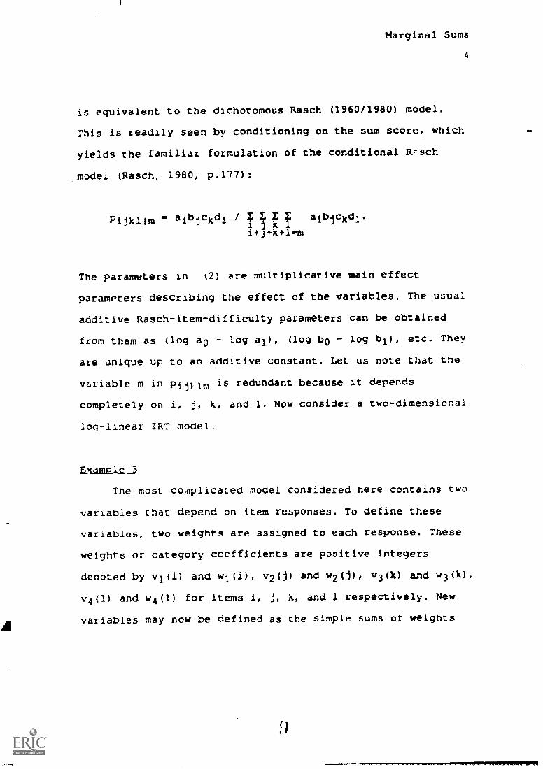
Let i, j, k, 1 = 0, I now be dichotomous item responses

and letmmitj*k+ 1, the simple sum of item scores, be

a new variable. Several authors (e.g. Cressie & Holland,

1983; Kelderman, 1984) have shown that the model

Pijklm = aibjckdlem

Marginal Sums

4

is equivalent to the dichotomous Rasch (1960/1980) model.

This is readily seen by conditioning on the sum score, which

yields the familiar formulation of the conditional R7sch

model (Rasch, 1980, p.177):

aibjckdl.Pijklimmaibjckdl IfIffi+1+k+lom

The parameters in (2) are multiplicative main effect

paramPters describing the effect of the variables. The usual

additive Rasch-item-difficulty parameters can be obtained

from them as (log a() log al), (log 1)0 - log bi), etc. They

are unique up to an additive constant. Let us note that the

variable m in pij)1m is redundant because it depends

completely on i, j, k, and 1. Now consider a two-dimensional

log-linear 1RT model.

Example 3

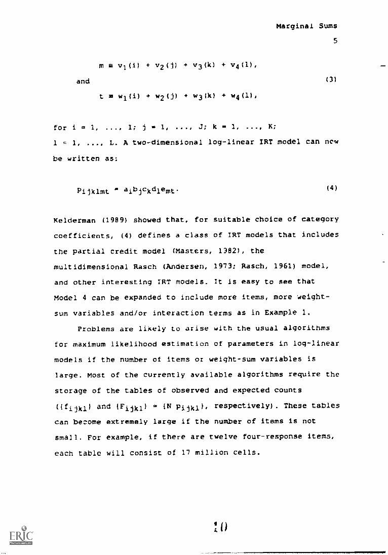
The most cooplicated model considered here contains two

variables that depend on item responses. To define these

variables, two weights are assigned to each response. These

weights or category coefficients are positive integers

denoted by v1(i) and wl(i), v2(j) and w2(j), v3(k) and w3(k),

v4(l) and w4(1) for items i, j, k, and 1 respectively. New

variables may now be defined as the simple sums of weights

Marginal Sums

5

m m v1(i) + v2(1) + v3(k) + v4(1),

and (3)

t m wl(i) + w2(j) + w3(k) + w4(1),

for i = 1, ..., I; j = 1, J; k 1, K;

1 - 1, ..., L. A two-dimensional log-linear IRT model can new

be written as:

Pijklmt aibjekdiemt. (4)

Keldermao (1989) showed that, for suitable choice of category

coefficients, (4) defines a class of IRT models that includes

the partial credit model (Masters, 1382), the

multidimensional Rasch (Andersen, 1973; Rasch, 1961) model,

and other interesting IRT models. It is easy to see that

Model 4 can be expanded to include more items, more weight-

sum variables and/or interaction terms as in Example 1.

Problems are lixely to arise with the usual algorithms

tor maximum likelihood estimation of parameters in log-linear

models if the number of items or weight-sum variables is

large. Most of the currently available algorithms require the

storage of the tables of observed and expected counts

((fijkil and (Fijkl) (11 Pijkl), respectively). These tables

can become extremely large if the number of items is not

small. For example, if there are twelve four-response items,

each table will consist of 17 million cells.

Marginal Sums

6

The algorithms described below avoid this problem by

computing the parameters directly from certain marginal sums

of the contingency table. The next section describes two such

algorithms: a modified version of the iterative proportional

fitting algorithm, and a version of the Newton-Raphszm

algorithm. Furthermore, an efficient method to calculate the

expected marginal sums is described at the end of the next

section. In the applications section, the computational

efficiency of this method is assessed, and the modified IPF

algorithm is applied to a set of simulated data.

Description

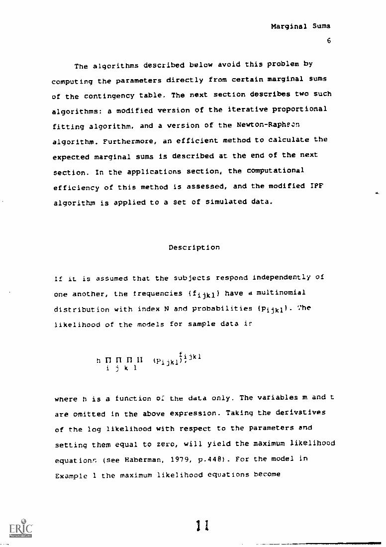
If it is assumed that the subjects respond independently of

one another, the frequencies If.-ijkl) have d multinomial

distribution with index N and probabilities I.Pijkl). The

likelihood of the models for sample data if

th n ijkln nil (p),ijkl

where n is a function or the data only. The variables m and t

are omitted in the above expression. Taking the derivatives

of the log likelihood with respect to the parameters and

setting them equal to zero, will yield the maximum likelihood

equationn (see Haberman, 1979, p.448) . For the model in

Example 1 the maximum likelihood equations become

11

fij++ = 0,

f+jk+ - = 0,

f++k1 F++kl 0,

Marginal Sums

i = 1, I;

j= 1, ..., J.

j= 1, ..., J;k 1, ..., K.

k = 1, K;

1 = 1, ..., L.

7

(5)

where a plus sign replacing an index denotes summation over

that index (e.g.Fij" = f Fijkl). The marginal sums

(fij"), If+ji"), and if++kl) are minimal sufficient

statistics for the parameters (aij), (bjk), and (cki)

respectively. Generally, in log-linear model analysis, the

sufficient statistics associated with par leters are the

marginal sums with the same indices as the corresponding

parameters. Furthermore, the likelihood equations are

obtained by setting the observed sufficient statistics equal

to the corresponding expected values under the model. Thus,

for Model 2, the likelihood equations are obtained by setting

the marginal sums (fi++++), ff+j"), (t"k+4), ff++.4.14.) and

(f++,+m) equal to the corresponding expected values

(F4A++), (F4.4.4.1.0 and (F++++ml.

Solving the Equations (5) for the parameters yields the

maximum likelihood estimates of the parameters. These

equations can not be solved directly, but numerical

algorithms are available for ...heir solution (e.g. Baker &

Welder, 1978, Goodman & Fay, 1974)

I 2

Marginal Sums

8

A Modified Iterative Proportional Fitting Alaorithm

In iterative proportional fitting (IPF, Deming

Stephan, 1940), the expected cell counts (Fijkl) are

proportionally adjusted to fit the set of marginal sums

obtained from the sample. In this section we describe a

modified IPF algorithm to adjust parameter estimates rather

th3n expected cell frequenries. This modification alleviates

b)th storage requirements and computational complexity

because test-data models usually have much less parameters

than expected frequencies.

Let us consider regular IPF. Denoting the expected

counts before the adjustment as (Pi(old)

) and after

adjustment as iFInew)*1jkl ,

start the computational procedure

(old)by setting all Fi jkl = 1. In IPF, the maximum likelihood

A

estimates (F-ijkl) under Model 1 are obtained by repeated

application of the adjustments

:.(new)rijkl

;.

rijkl

"(new)Fijkl

=

'

=

;(old)rijkl

l(new)

".(old)ijkl

"(old)Fijki

,,l'ij++

,,%'+jk+

(f++kl

/

,

/

-(0.1d)Fij4.4. )

;(old),

"(old)F++kl )

each for i = 1, ..., I; j = 1, ..., J; k = 1, ..., K;

1 = 1, L, until convergence is achieved. The algorithm

will always converge to a solution satisfying Equations 5.

The application of IFF to other models, such as those given

in Example 2 and 3, is straightforward.

To adjust parameter estimates rather than expected cell

1 3

Marginal Sums

9

frequencies, let us first express Fi jkl in terms of

parameters. For the first update, this becomes

al3ew)blvw)ci(rliew) = N a1,31d)birtld)4T1d)(fil++IFIVI))

(old)Because the same adjustment (fij,"/Fij++ ) is made for ail

values of k and 1, it suffices to change thp parameter aij

only. The remaining parameters bjk and cki can be treated as

i (old)constants so that b(new)jk

(new)= bold)jk cid. Therefore, we

have

(new) (old) ,, ,v(old),aij = aij to = 1/ .../ 1;

j= 1, - , J,

Similarly for the other updates, we have

and

blrw) bliocld) (f+ik+/E.Vcd) j= 1, . . , J.k = 1, K,

(new) (old) , (old), ,

ckl = ckl "++klfr/,++kl /, = 11 K,

1 = 1, ..., L.

Within the modified IFF algorithm, only IJ + JK + XL

parameters have to be adjusted in one cycle. Compared to the

1 4

Marginal Sums

10

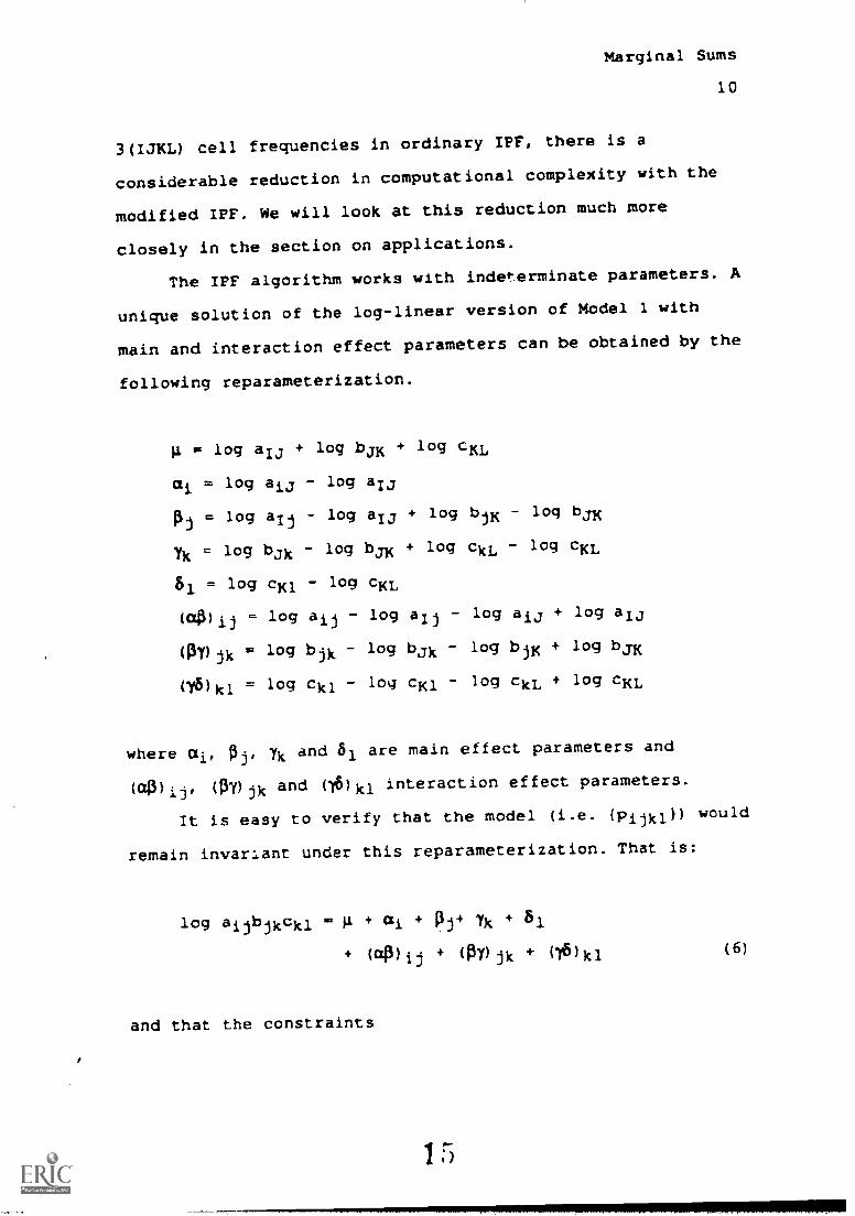
3(IJKL) cell frequencies in ordinary IPF, there is a

considerable reduction in computational complexity with the

modified IPF. We will look at this reduction much more

closely in the section on applications.

The IPF algorithm works with indeterminate parameters. A

unique solution of the log-linear version of Model 1 with

main and interaction effect parameters can be obtained by the

following reparameterization.

g is log a/j + log bjK + log cKL

ai = log aij - log aIj

pj . log a/j - log a13 + log bjK loq bjK

yk = log bjk log bjK + log cud - log cm,

51 = log cK1 - log cm,

(aP)ij = log aij - log a/j log aij + log aIj

(Py)jk = log bjk log bjk - log bjK + log bjK

OCkl = log ckl log cK1 - log ckL log cm,

where ai, pj, yk and 81 are main effect parameters and

(ap)ij, (py)jk and 0(8) k1 interaction effect parameters.

it is easy to verify that the model (i.e. (.Pijkl)) would

remain invariant under this reparameterization. That is:

log ai-b3 jkckl A 4" ai Pj+ Ick 51

+ (4)1 i + (Prjk + 045)kl

and that the constraints

1 5

(6)

al ' 13.7 = YK = 8L = (aA)Ij = (4)ij

= *Pa = (78)/(1 (16)kL =

marginal Sums

11

(7)

are satisfied.

This parameterization contrasts the effect of each

category with the last. Bock (1975, p.239) refers to this as

the 'simple contrast'. Other parameterizations such as

deviation contrasts, where the effect of each category is

contrasted with the mean effect, can be obtained by similar

transformations.

A Newton-Raphsgh Algorithm

The well-known Newton-Raphson algorithm is based on a

second order Taylor expansion of the log-likelihood function

(Andersen, 1980, p. 47; Adby & Dempster, 1974, p. 65). The

a1g,).,_±thm iteratively computes the log-linear parameters

using the gradient and the Hessian matrix, which can be

written as functions of the marginal sums. Before discussing

the Newton-Raphson (N-R) update, let us first introduce the

matrix formulation of the log-linear formulation given in (6)

for Model 1:

log Pijkl m g ai Pj Yk 4' 81

+ opij + (PT)jk 04)kl-

Marginal Sums

12

Without loss of generality, let us assume that1=J=K= L

= 2. Unlike TPF, the N-R algorithm requires the parameters to

be identified. Therefore we impose the constraints given in

(7). Let p IP1111, P2111, P2222)' be the vector of=

1, , , (4)11,01 11' 81cell probabilities, and let4 = (u ft

(131)11, (0)11)' be the vector of parameters to be estimated.

The matrix version of the model can be written as

log p = D k,

where D is the design matrix with ones and zero's in the

appropriate places and log means the elementwise logarithm

operator. Letting f = (f1111, f2111, f2222) and A =

diag(p), the gradient vector and the Hessian matrix can be

expressed as

and

a log L

a k

D'f D'pN

a2 log L= N(D'ApD (D'p) (D'W] .

a t a t,

respectively.

since

These can alsr be expressed in terms of marginal sums

1 7

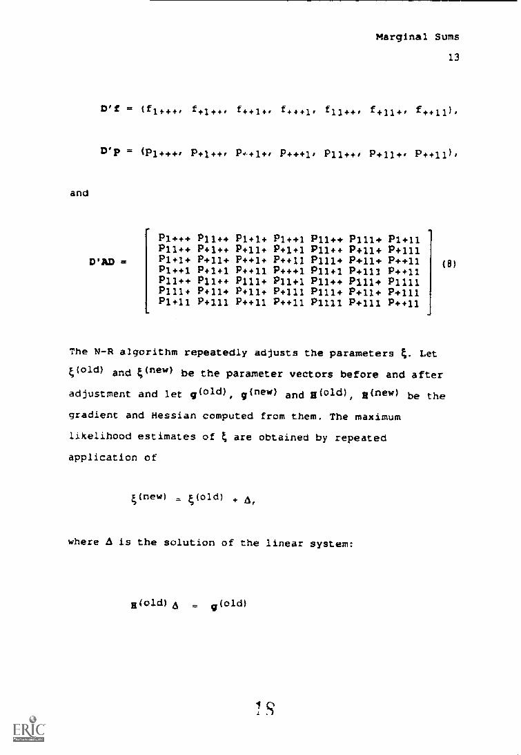
and

Marginal Sums

13

D'f = (f1+++, f+14.4., 4+1+, 44+1, fll++, f+11+, f++11),

D'p = (P1+++, P4.+1+, P+++1. All++. P+11+, P++11),

D'AD

Pl+++ P11++ P1+1+ Pl++1 P11++ P111+ P1+11P11++ P+1++ P+11+ P+1+1 P11++ P+11+ P+111P1+1+ P+11+ P++1+ P++11 P111+ P+11+ P++11P1++1 P+1+1 P++11 P+++1 P11+1 P+111 P++11P11++ P11++ P111+ P11+1 P11++ P111+ P1111P111+ P+11+ P+11+ P+111 P111+ 13+11+ P+111P1+11 P+111 14+11 14+11 P1111 P+111 P++11

(8)

The N-R algorithm repeatedly adjusts the parameters 4. Let

4(old) and 4(new) be the parameter vectors before and after

adjustment and let g(new) and EI(Old), R(new) be the

gradient and Hessian computed from them. The maximum

likelihood estimates of t are obtained by repeated

application of

(new) = 4(01d) + A,

where A is the solution of the linear system:

1(01d),5 g(old)

Marginal Sums

14

Usually the update A is computed by pre-multiplication of

system the by the inverse of B(01d), but it is more efficient

to solve the system directly for A (Dongarra et al, 1979;

Holland & Thayer, 1987). Gill, Murray and Wright (1991)

describe fast methods for solving systems of linear

equations. The Newton Raphson algorithm converges much more

rapidly to the maximum likelihood solution than the IPF

algorithm but requires starting values that are close to the

final solution. Also a requires the marginal sums given in

(8), which are not necessary for the modified IPF algorithm.

The most important feature of the above modifications of

the IPF and N-R algorithms is that in neither case is it

necessary to set up the full contingency table. Marginal sums

alone are sufficient. Although this reduces storage,

requirements it does not relieve us of the computational

burden of summing over the cells of the full table, which is

probably the reason why the above N-R procedure is never used

in existing programs for log-linear analysis. A novel element

in the application of the N-R algorithm and modified IPF, is

that the marginal sums are computed in an efficient way

described in the next section.

Efficient COMPUtation Qf Marginal Sums

cells

The obvious way to compute (Fij+4.) is to sum over the

F. =NEEPijkl13++ =NEEaijbjkckl,k 1 k 1

( 9

Marginal Sums

15

i 1, ..., I, j = 1, J, where the last term is used to

avoid storage of the full table.

Suppose that I = J = K = L = 10, then (9) involves

2(IJKL) + 1 = 20,001 multiplicatioTts and IJ(KL - 1) = 9900

summations. This number of computations can be reduced by

rewriting (9), using the distributive law of multiplication

over summation, as

Fij" m N aij bjk I ckl,

i = 1, ..., I, j = 1, ..., J.This requires only 1 + 1J + K =

111 multiplications and J(K-1) + K(L-1) = 180 summations.

This is obviously a considerable reduction in the number of

computations needed.

we will refer to this method of computing the expected

marginal sums as the marginalization-by-variable (MBV)

method, because summations for one variable (at a time) are

done only over parameters that depend on that variable.

Multiplication with parameters that do not depend on that

variable is postponed until after the summation.

The MBV method becomes more complicated if the model

contains weight-sum variables, because they are dependent on

item responses (e.g. Example 3). In that example, the values

that a summation in the MBV method can take, may depend on

the value of other summation variables. For example, the

computation of F++.1.4.m in Model 2, can be written as

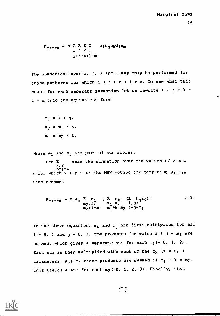
Marginal Sums

16

=WEI aibjckdlemijkli+j+k+1=m

The summations over i, j, k and I may only be performed for

those patterns for which i + j + k + 1 = m. To see what this

means for each separate summation let us rewrite I + j + k +

1 a m into the equivalent form

/111 E if

M2 E 1111 k,

m m2 10

where ml and m2 are partial sum scores.

Let 2 mean the summation over the values of x andx,yx+r=z

y for which x + y = z; the MBV method for computing p.4.4.4.4.m

then becomes

Ffmm N em 1 d1 ( L ck a bjal)) (10)

m2,1; ml,k; i/j;m2+1111 m1+km2 i+j=m1

In the above equation, ai and bj are first multiplied for all

i = 0, 1 and j 0, 1. The products for which i + j ml are

summed, which gives a separate sum for each m1(= 0, 1, 2).

Each sum is then multiplied with each of the ck (k = 0, 1)

parameters. Again, these products are summed if mi + k m2.

This yields a sum for each m2(=0, 1, 2, 3). Finally, this

Marginal Sums

17

process of multiplication and summation is repeated one more

time to obtain F4.4.4.4.m. In this way, the marginal sums are

computed efficiently while, at the same time, avoiding

summation over logically impossible combinations of variable

values.

In a similar manner, the marginal sums for the model in

Example 3 can also be computed. First, rewrite the weight-

sums given in (3) as

m1=v1(i)+v2(j), m2=1711"3(k), m=1712+1'4(1)

tls=w1(i)+w2(J), t2=t1+w3(k); t-t2+w4(1)

Under these constraints, the marginal sum p+++,mt can be

computed as

F+4.44mt = N emt E d1 a ck (L bjai)).1,m2,t2 k,m1,t1 i,j

Again each summation can be performed separately if the

constraints in (11) are respected. Obviously, the same method

can be applied to calculate the other expected marginal sums

such as (Fi+++++), (F+J+++.0, etc. Consequently, the miav

method can supply all marginal sums needed in the modified

IPF or N-R algorithm.

The modified IPF algorithm using the MBV method to

compute expected marginal sums, is implemented in the

computer program called LOGIMO (LQGlinear IRT Wdeling,

r) 91.

Marginal Sums

18

Kelderman & Steen, 1988). LOGIMO is a Pascal program that

estimates log-linear models with main and interaction effect

parameters of item response, backgroun..4 variables and one or

more weight-sum variables as shown in Example 3. The weights

are integer valued and must be specified by the user. In the

next section we present the application of the modified IPF

and N-R algorithm.

Application

The complexity of computing the parameters of log-linear

models is substantially reduced by using modified IPF and N-R

algorithms based on marginal sums that can be computed

efficiently by the MBV method. In this section we will

examine the computational complexity as a function of the

number of variables in the model. We will first look at the

increase in computational complexity with the MBV algorithm

and then at the full algorithm.

In this application, we restrict our attention to the

IPF algorithm and to the simplest model with sum scores as

given in (2). This model is chosen because the number of MBV

computations is tractable and because it is equivalent to the

di;thotomous Rasch model. Consequently the parameter estimates

can be compared to those of an existing algorithm for

computing Rasch parameters and to verify the correctness of

the algorithm.

23

Marginal Sums

19

Insert Table 1 here

In Table 1, the numbers of summations and

multiplications in the computation of F4....+1/1 of the simple

sum-score model (2) are given for five to 20 items. It can be

seen that for the MIMI algorithm these numbers remain within

reasonable limits, whereas, for the case of summing over all

cells (9), these numbers increase very rapidly.

To evaluate the full IFF algorithm, test data conforming

to the Rasch model were generated for 20 items. The item

difficulties where randomly chosen from the uniform

distribution over the interval (-2,2). Latent trait values

for 10,000 cases were drawn from a uniform distribution over

the [-3,31 interval. Log-linear kasch models given in (2)

were then fitted to these data. Nine computer runs were made

for different subsets of items, where the first subset

contained the first four items, the second subset contained

the first six items etc. In Figures 1, 2, and 3, different

statistics of these runs are plotted against the number of

items in the model.

Insert Figures I, 2 and 3 about here

2.4

Marginal Sums

20

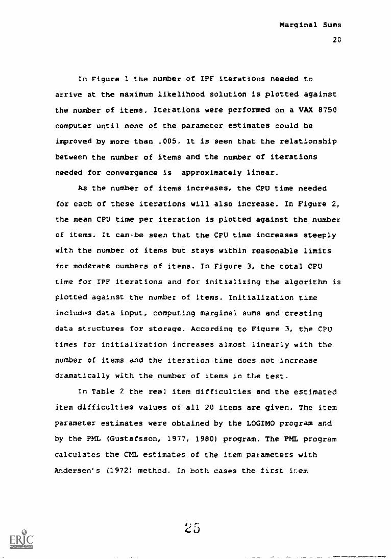
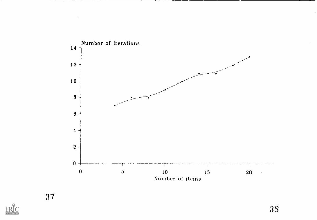
In Figure 1 the number of IPF iterations needed to

arrive at the maximum likelihood solution is plotted against

the number of items. Iterations were performed on a VAX 8750

computer until none of the parameter estimates could be

improved by more than .005. It is seen that the relationship

between the number of items and the number of iterations

needed for convergence is approximately linear.

As the number of items increases, the CPU time needed

for each of these iterations will also increase. In Figure 2,

the mean CPU time per iteration is plotted against the number

of items. It can-be seen that the CPU time increases steeply

with the number of items but stays within reasonable limits

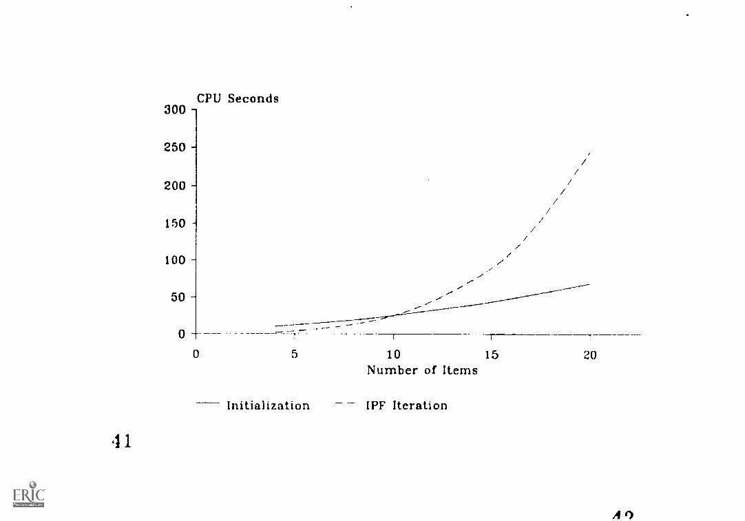
for moderate numbers of items. In Figure 3, the total CPU

time for IPF iterations and for initializing the algorithm is

plotted against the number of items. Initialization time

includes data input, computing marginal sums and creating

data structures for storage. According to Figure 3, the CPU

times for initialization increases almost linearly with the

number of items and the iteration time does not increase

dramatically with the number of items in the test.

In Table 2 the real item difficulties and the estimated

item difficulties values of all 20 items are given. The item

parameter estimates were obtained by the LOGIMO program and

by the PML (Gustafsson, 1977, 1980) program. The PML program

calculates the CML estimates of the item parameters with

Andersen's (1972) method. In both cases the first item

MaLginal Sums

21

difficulty parameter was set equal to its real value.

Furthermore, the iterations were stopped until none of the

parameter estimates could be improved by more than .0001. It

can be seen from Table 2 that both solutions are identical up

to the second decimal place, indicating that the IPF/MBV

algorithm correctly calculates maximum likelihood estimates.

Insert Table 2 here

Finally a note on the usefulness and availability of

LOGIMO. For ordinary log-linear models, provided they are not

too complicated, LOGIMO makes it possible to analyze larger

numbers of variables than with other programs. For certain

special Rasch models such as (2), dedicated programs such as

RIDA (1989), and PML will generally be faster. If, however,

the user wants to define his of her own IRT model with

several dimensions and/or user specified category

coefficients, LOGIMO is the way to go. LOGIMO is a Pascal

program that runs VAX system running under VMS. For smaller

problems there is a PC version (386, with extended memory).

LOGIMO will be distributed starting somewhere in the summer

of 1992 by iec PrcGAMMA, P.O.Box 841, 9700 AV Groningen, The

Netherlands (E-mail: GAMMA@RUG.NL).

2 ti

, .41111111111111111411111.1

Marginal Sums

22

Discussion

In this paper an efficient algorithm is described that

calculates the parameter estimates of log-linear models

including log-linear IRT models. The :"..gorithm avoids setting

up the full Item 1 x x Item k table by computing the

parameter estimates from the marginal-sums of the table by a

modified version of the iterative proportional fitting

algorithm or the Newton-Raphson algorithm. The computation of

expected marginal sums is done efficiently using the MBV

method.

The methods modified IPF and MBV methods can be seen as

generalizations of older methods for the estimation of

unidimensional Rasch models. For this case, the modified IFF

algorithm turns out to be equivalent to an algorithm proposed

by Scheiblechner (1971, see Fischer, 1974, p.247) and the MBV

method can be shown to be identical to the so called

summation algorithm for the computation of elementary

symmetric functions (Andersen, 1972) . To see the latter,

normalize the parameters in the Rasch model (2) as ao = 130 =

co = do = 1. Elementary symmetric functions can then be

computed recursively using the following type of relations

16(alfbifc1fdl) = Im(airbi,C1) + d1 ym-i(al,b1,c1),

and similar relations for 7in(a11b11c1), ylm(al,b1), etc.

Marginal Sums

23

It is easy to see that this summation is equivalent to the

left-most summation in (10), and ym(al,b1,c1) and

7m_1(al,b1,c1) are equivalent to the second summation in

(10). Thus, the MBV method for computing marginal sums in the

Rasch model is equivalent L:le summation algorithm for

computing elementary symmetric functions. Despite this for

unidimensional Rasch models LOGIN°, is genererally slower than

programs using the sum algorithm that arc dedicated to those

models. As remarked before its streno* Jies in ordinary log-

linear models and more complicated log-linear IRT models.

LOGIMO is capable of dealing with models with

interaction terms and multiple weight-sum variables with

arbitrary weights defined by ne user. In these models the

nice symmetries of the Rasch model are lost. It is an open

question whether improved methods for computing elementary

symmetric functions, such as those of Formann (1986) and

Verhelst, Glas and van der Sluis (1984), depend on these

symmetries or and/or can be generalized for use with general

log-linear models.

Marginal Sums

24

References

Adby, P.R. & Dempster, M.A.H. (1974). Introduction to

optimization methods. London: Chapman and Hall.

Agresti, A. (1984). anguyaja.si_azdinalsatrisajararaLcar.a. New

York: Wiley.

Andersen, E.B. (1972) . The numerical solution of a set of

conditional estimation equations. aaurnal_al_Lha_Baxal

Statistical qpciety it, 1A, 42-54.

Andersen, E.B. (1973) . Conditional inference and multiple

choice questionnaires. BLItish_jszmnaLstiltlathematical

and Statistical Psychology, 26, 31-44.

Andersen, E.B. (1980). Discrete statistical models wiLh

agslal_sr-ituag.L.lualicat_igns. Amsterdam: North Holland.

Baker, R.J., & Nelder, J.A. (1978). 1121!aLLti_symt&"

Generalized linear interactive modeling. Oxford: The

Numerical Algorithms Group.

Bock, R.D. (1975) thatixarlat_e_atfulaticsu_meamds_in

Dehavioral research. New York: McGraw Hill.

Cressie, N., & Holland, P.W. (1983). Characterizing the

manifest probabilities of latent trait models.

EsychometrakA, la, 129-142.

Deming, W.E., & Stephan, F.F. (1940). On a least squares

adjustment of a sampled frequency table when the

expected marginal totals are known. Annals of

Mattematical_Statis_tica, 11, 427-444.

t7PY .1!AILASILE

2;)

Marginal Sums

25

Dongarra, J.J., Bunch, J.R., Moler, C.B., and Stewart, G.W.

(1979) LINPACK _users' auidft. Philadelphia, PA: SIAM.

Duncan, O.D. (1984). Rasch measurement: Further examples and

discussion. In C.F. Turner 6 E. Martin (Eds.), Surveying

subjective phenomena. Vol. 2 (pp. 367-403). New York:

Russell Sage Foundation.

Duncan, 0.D., 6 Stenbeck, M. (1987). Are likert scales

unidimensional? 5ocia1 Science ResearCh, lfi, 245-259.

Fischer, G.H. (1974). Einführung in die Thecrie

ossichologischer Testa (IntroductinA to the theory of

psychological tests) . Bern: Huber (In German).

Formann, A.K. (1986) . A note on the computation of the

second-order derivatives of the elementary symmetric

functions in Rasch models. rsychometrika, 51, 335-339.

Gill, P.E., Murray, W., & Wright, M.H. (1991). Numerical

linesu_algentrja_and_satimizatlan. Redwood City: Addison

Wesley.

Glas, C.A.W., (1989). ratdniatioa_ansLussaasuaaaraLmagirja,

Unpublished Doctoral Dissertation, University of Twente.

Enschede the Netherlands. (ISBN 90-9003078-6)

Goodman, L.A., & Fay, R. (1974). ECIA_REasmam,_dlaardataan

for users. Chicago: Department of Statistics University

of Chicago.

Gustafsson, J.E. (1977). The Rasch_AosieLiar_sachotomous

Reports from the Institute of Education, University of

Goteborg, nr. 85.

3 0

Marginal Sums

26

Gustafsson, J.E. (1980) . A solution of the conditional

estimation problem for long tests in the Rasch model for

dichotomous items. Educational and Psychological

Measurement, 40, 377-385.

Haberman, S.J. (1979). Analysis of aualitative data: _New.

developments- Vol. 2. New York: Academic Press.

Holland, P.W. & Thayer, D.T. (1987). Notes on the use of loci-

linear-imials_taLlisting_slimczateLztzniatiailitadialLuautu2na. (Technical Report No. 87-79). Princeton,

NJ: Educational Testing Service.

Kelderman, H. (1984) . Loglinear Rasch model tests.

Psvchomatrika, A2, 223-245.

Kelderman, H. (1989a). Item bias detection using loglinear

IRT. Psychometrika, ig, 681-698.

Kelderman, H. (1989b). Lasaiagaz_Ealauxuallaaajoui_ux_macteis

for polvtomouslv scpred items. paper read at the Fifth

International Objective Measurement Workshop, Berkeley,

march 26.(ERIC document Reproduction Service No. ED 308

238))

Kelderman, H. (1991) . Estimating and tearing a

multidimensismaL_Baszh_mpsie.L.lar-__PAISIAL:reslitar.sazinapaper read at the Annual Meeting of the American

Educational Reseach Association, Chicago Ill, April 5.

(In review)

Kelderman, H., & Steen, R. (1988) . LOGIMO: Loglinear IRT

dadeling (Program Manual]. Enschede, The Netherlands:

University of Twente.

31

Marginal Sums

Masters, G.N. (1982). A Rasch model for partial credit

scoring. zushmletzika, Ai, 149-174.

Rasch, G. (1960). -$

27

_4

And_Attainment_testa. Copenhagen: Paeda)giske Institut.

Rasch, G. (1961) . On general laws and the meaning of

measurement in psychology. EzaQanding2_21_1jogi_gaumh

PI .1 t =

probabilitx, 1, 321-333.

Basch, G. (1980) . Z.Lotabillatir.mosleaz_igirgilm2_int.e.iliagrae

And attainment tests. Chicago: The University of Chicago

Press.

Scheiblechner, H. (1971). a simple algorithm for CML-

model with two or more categories of answers. Research

Bulletin Nr. 5/71, Psychological Institute, University

of Vienna, Austria.

SPSS, Inc. (1988). 51'55 Uger's Guide (2rd Edition). Chicago,

IL: SPSS, Inc.

Tjur, T. (1982) . A connection between Rasch's item analysis

model and a multiplicative Poisson model. 5candinavian

11"411611--C21--aitalLiatagia, 2, 23-30.

verhelst, N.D., Glas, C.A.W., Sluis, A. van der. (1984).

Estimation problems in the Basch model: The basic

symmetric functions.

1, 245-262.

3

Marginal Sums

28

Author Notes

The author thanks Wim J. van der Linden, Gideon J.

Mellenbergh and Namburi S. Raju for their valuable comments

and suggestions. Requests for reprints should be sent to:

University of Twente, Bibliotheek, P.O. Box 217, 7500 AE

Enschede, The Netherlands.

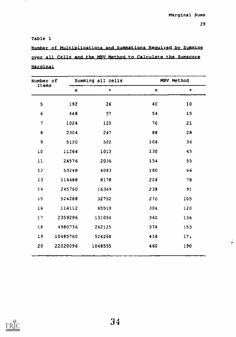
Table 1

11

Marginal Sums

29

1!6 - I I11

NumberItems

of Summing all cells MBV Method

5 192 26 40 10

6 448 57 54 15

7 1024 120 70 21

8 2304 247 88 28

9 5120 502 108 36

10 11264 1013 130 45

11 24576 2036 154 55

12 53248 4083 180 66

13 114688 8178 208 78

14 245760 16369 238 91

15 524288 32752 270 105

16 114112 65519 304 120

17 2359296 131054 340 136

18 4980736 262125 378 153

19 10485760 524268 418 171

20 22020096 1048555 460 190

34

Marginal Sums

30

Table 2

ileAL_ancLEatimatest_itent_DiffisaltiesLiQLfiimulatziaasA

ilifazsasa

Item

1 2 3 4 5Real .858 -1.512 -0.173 -1.040 1.137LOGIMO .858* -1.517 -0.214 -1.069 1.161PM1 .858" -1.517 -0.215 -1.069 1.161

6 7 8 9 10

Real 1.354 1.690 0.577 -1.270 -0.155LOGIMO 1.318 1.636 0.618 -1.350 -0.154PML 1.318 1.636 0.618 -1.349 -0.153

11 12 13 14 15

Real 1.302 1.352 -0.823 -0.883 -1.754LOGIMO 1.243 1.282 -0.858 0.871 -1.801PM1 1.244 1.284 -0.857 0.871 -1.801

16 17 18 19 20

Real -0.026 0.221 0.517 -0.460 1.658LOGIMO -0.038 0.183 0.502 -0.506 1.654PML -0.038 0.183 0.502 -0.507 1.653

*) The estimated parameter of the first item was set equal

to the real parameter value to fix the scale

35

Marginal Sums

31

Figure Captions

riaure 1. Growth of the Number of IPF Iterations with the

Number of Items in Model 2.

Figure 2. Growth of CPU Time per Iteration with the Number of

Items in Model 2.

figure 3. Growth of CPU Time for Initialization and IPF

Iterations with the Number of I terns in Model 2.

Number of Iterations14 -,

12 -

10 -

6 -

4

2

37

_._,.._--.------

.---"---

5 10 15Number of items

20

38

CPU Seconds20

15

10

5

0

3 !)

//0 5 10 15

Number of Items

4 0

300 -

250

200

150

100 -

50 -

0

CPU Seconds

----r------.7.7---

i...,,-

--T 1

0

4 1

/7

/

//

5 10Number of Items

Initialization IPF Iteration

I

15 20

A 1

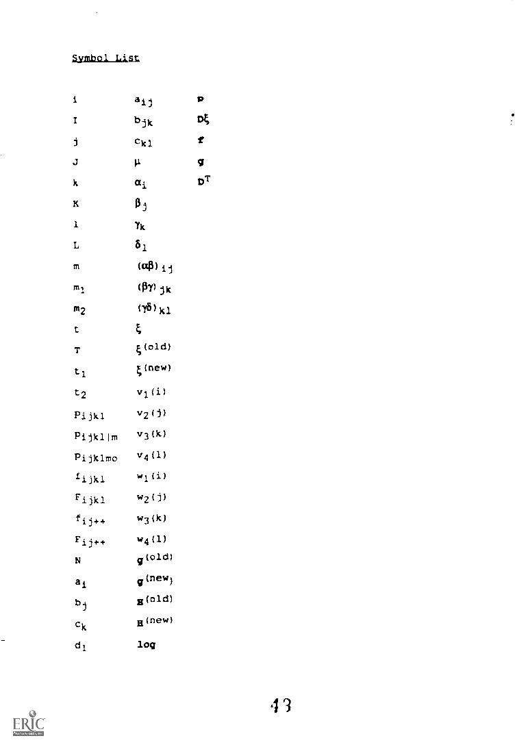
5ymbol List

i ajj1 bjk

j ckl

J P

k ai

K

1 Yk

L 51

m (4) ij

mi (Pr jk

m2 (75) kl

t k

T (old)

ti (new)

t2 v1(i)

Pijkl v2(j)

Pilk1Im v3(k)

Pijklmo v4(1)

lijkl nal

Fijkl w2(j)

fij++ w3(k)

Fii++ w4(1)

N g(old)

ai g (nevi)

bj R(old)

ck Ii(new)

d1 log

p

D4

f

g

DT

4 3

lEuizar.aita.stiZzoras,fauslinsing.

RR-91-1 H. Kelderman, Computing Maximum Likelihood Estimates of

Loglinear NtiodOls from Marginal Sums with Special Attention to

Loglinear Item Response Theory

RR-90-8 M.P.F. Berger 6 D.L. Knol, On the Assessment of

Dimensionality in Multidimensional Item Response Theory

Medels

RR-90-7 E. Boekkooi-Timminga, A Method for Designing IRT-based Item

Blanks

RR-90-6 J.J. Adema, The Construction of Weakly Parallel Tests by

Mathematical Programmdng

RR-90-5 ;J.J. Adena, A Revised Simplex Method for Test Construction

Problems

RR-90-4 J.J. Adana, Methods and Models for the Construction of Weakly

Parallel Tests

RR-90-2 H. Tobi, Item Response Theory at subject- and group-level

RR-90-1 P. Nesters 6 H. Kelderman, Differential item functioning in

multiple choice items

Regearch &MOILS can be obtained at costs from Bibliotheek,

Department of Education, University of Twente, P.O. Box 217,

7500 AE Enschede, The Netherlands.

4 4

BEST COPY AVAILABLE

depactment ofa

EDUCATION..A publication by

the Department of Education

of the University of Twente

P.O. Ow 211