An Idealized Model and Systematic Process Study of OxygenDepletion in Highly Turbid Estuaries

S. A. Talke & H. E. de Swart & V. N. de Jonge

Received: 11 June 2008 /Revised: 15 April 2009 /Accepted: 19 April 2009 /Published online: 27 May 2009# Coastal and Estuarine Research Federation 2009

Abstract The sensitivity of oxygen depletion in turbidestuaries to parameters like freshwater discharge, depth,and sediment availability is investigated using an idealizedmodel. The model describes tidally averaged circulation andsuspended sediment concentration (SSC), which are inputinto an advection–diffusion sink module of dissolvedoxygen (DO). Based on the analysis of field data collectedin the Ems estuary, the modeled oxygen depletion rates areproportional to SSC. The model is calibrated to the observedvariation of DO with SSC and temperature. Modeled DOclosely tracks changes to the estuarine turbidity zone (ETZ):increased channel depth, decreased freshwater discharge,and decreased mixing move the ETZ upstream, amplifySSCs, and decrease DO. Summertime temperatures producelower DO than cooler periods. Model results are consistentwith historical measurements in the Ems, which indicate thathypoxic events (DO concentrations<2 mg l−1) have oc-curred more frequently after deepening from 5 to 7 m.

Keywords Estuarine circulation . Estuarine turbiditymaximum . Sediment dynamics . Morphology . Fluid mud .

Water quality . Hypoxia . Anoxia . Ems estuary

Introduction

Depleted levels of dissolved oxygen (DO) occur in manyAsian estuaries (Fang and Lin 2002; Dai et al. 2006; Ni etal. 2007), North American estuaries (Engle et al. 1999;Borsuk et al. 2001; Hagy et al. 2004; Benoit et al. 2006;Lin et al. 2006), and European estuaries (Uncles et al. 1998;Garnier et al. 2001). These zones of hypoxia (DOconcentration<2 mg l−1) greatly degrade environmentalconditions for benthic and pelagic fauna and alter redoxconditions, which changes the cycling of nutrients andpartitioning of pollutants throughout the estuary (de Jongeand Villerius 1989; Diaz and Rosenburg 1995; Nestlerodeand Diaz 1998; Fang and Lin 2002). Given the ecologicalconsequences of hypoxic and anoxic conditions, there is astrong need to understand, on a process level, the physicaland biological processes that are contributing to thisproblem.

In many estuaries, oxygen depletion is tied to the inputsof organic matter caused by effluent, industry, or naturalcauses (Hagy et al. 2004; Dai et al. 2006; Fang and Lin2002; Wei et al. 2007). Other estuaries such as the HumberEstuary, Loire Estuary, and Yellow River Estuary showevidence of oxygen depletion due to the degradation oforganic matter that is associated with the suspendedsediment aggregates (Uncles et al. 1998; Thouvenin et al.1994; Ni et al. 2007). Physical processes which affect DOconcentrations include vertical mixing and stratification,river discharge, and baroclinic circulation. In the Ches-apeake Bay region, high river inflow causes greater influx

Estuaries and Coasts (2009) 32:602–620DOI 10.1007/s12237-009-9171-y

Electronic supplementary material The online version of this article(doi:10.1007/s12237-009-9171-y) contains supplementary material,which is available to authorized users.

S. A. Talke (*)Civil and Environmental Engineering Department,University of Washington,201 More Hall, Box 352700, Seattle, WA 98195-2700, USAe-mail: stalke@u.washington.edu

H. E. de SwartInstitute for Marine and Atmospheric research, Utrecht University,Princetonplein 5,3584 CC Utrecht, the Netherlandse-mail: h.e.deswart@uu.nl

V. N. de JongeInstitute of Estuarine Coastal Studies (IECS), University of Hull,Hull HU6 7RX, UKe-mail: v.n.de.jonge@planet.nl

of nutrients, greater primary production, and subsequentdepletion of DO (Hagy et al. 2004; Lung and Nice 2007).In other estuaries, hypoxic conditions occur during low-inflow conditions and are attributed to the increasedresidence time of water (Dai et al. 2006; Hagy and Murrell2007). Vertical mixing often controls DO, with depletionoccurring in highly stratified systems (Borsuk et al. 2001;Lin et al. 2006; Hagy and Murrell 2007). Finally, anidealized analytical model and a box model show thatgravitational circulation, which drives near-bed flows ofoxygenated seawater into the estuary, also alters the oxygenbudget of estuaries (Lin et al. 2006; Hagy and Murrell 2007).

In this paper, we investigate oxygen depletion thatoccurs in the estuarine turbidity zone (ETZ) of the Emsestuary. Before the 1980s, hypoxic conditions occurredprimarily in the Dollard subbasin from the discharge oforganic matter (e.g., sewage effluent), particularly whenlow freshwater discharge resulted in a large residence timeof water (Helder and Ruardij 1982). Though sanitationmeasures greatly reduced the organic load and oxygendepletion in the Dollard (Essink 2003), we present measure-ments which show that low DO concentrations areincreasingly being measured in the brackish and freshwaterportions of the river Ems, upstream of the Dollard. Using acombination of field measurements and modeling, weinvestigate the cause of the renewed water quality problem,focusing on the connection between depleted DO andincreased suspended sediment concentrations (SSCs) in theturbidity zone. The physical mechanisms behind decreasingDO concentrations and increased turbidity are investigated

with an idealized tidally averaged model that estimatescirculation, SSC (organic matter), and DO concentrations.Estuarine geometry, physical, and biological processes aresimplified to investigate first-order effects and result in amodel of oxygen depletion that is transparent, computa-tionally fast, and flexible. Using sensitivity studies, weidentify key parameters that govern observations. For turbidestuaries, we show that the along-channel distribution oforganic material—which is set by the sediment dynamics ofturbidity zones—governs the depletion of DO.

Observational Background

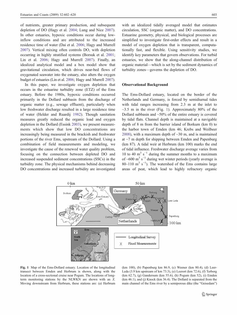
The Ems-Dollard estuary, located on the border of theNetherlands and Germany, is forced by semidiurnal tideswith tidal ranges increasing from 2.3 m at the inlet to~3.5 m in the river (Fig. 1). Approximately 80% of theDollard subbasin and ~50% of the entire estuary is coveredby tidal flats. Channel depth is maintained at a navigabledepth of 8 m from the barrier island of Borkum (km 0) tothe harbor town of Emden (km 46; Krebs and Weilbeer2008), with a maximum depth of ~30 m, and is maintainedat ~7 m depth for shipping between Emden and Papenburg(km 87). A tidal weir at Herbrum (km 100) marks the endof tidal influence. Freshwater discharge average varies from10 to 40 m3 s−1 during the summer months to a maximumof ~600 m3 s−1 during wet winter periods (yearly average is80–110 m3 s−1). The watershed of the Ems contains largeareas of peat, which lead to highly refractory organic

Fig. 1 Map of the Ems-Dollard estuary. Location of the longitudinaltransect between Emden and Herbrum is shown, along with thelocation of a cross-sectional cruise near Pogum. The locations of long-term monitoring stations by the NLWKN are shown with an X.Moving downstream from Herbrum, these stations are: (a) Herbrum

(km 100), (b) Papenburg km 86.9, (c) Weener (km 80.4), (d) Leer-Leda (3.9 km upstream of km 73.3), (e) Leerort (km 72.6), (f) Terborg(km 62.7), (g) Gandersum (km 55.6), (h) Pogum (km 52), (i) Emden(km 46.1), and (j) Knock (km 36.4). The Dollard is separated from themain channel of the Ems river by a semiporous dike (the “Geisedam”)

Estuaries and Coasts (2009) 32:602–620 603

material in the estuary (van Es et al. 1980; Baretta andRuardij 1988). Water temperature varies from 0°C to 25°Cbetween winter and summer.

We use a combination of moored monitoring data, andcruise data to analyze oxygen depletion. For the years2005–2006, salinity, SSC, temperature, freshwater dis-charge, and DO concentration measurements at 5–30-minincrements were made available at eight stations along theEms by the Niedersächsisches Landesbetrieb für Wasser-wirtschaft, Küsten-und Naturschutz (NLWKN), part of theGerman state of Niedersachsen (see Fig. 1). We also usehistorical measurements of salinity, DO, and temperaturefrom the stations at Leer-Leda (located 3.9 km upstream ofEms km 73.3 on the Leda tributary) and Terborg (km 62.7),which are available from 1984 to 2000 and 1988 to 2000,respectively, from the NLWKN. Historical measurements ofturbidity and SSC are available at Leer-Leda and Terborg,respectively, from 1998 to 2000.

Beginning in February 2005 and running throughDecember 2007, 30 (nearly) monthly measurements ofwater quality and biological parameters were made alongthe longitudinal axis of the Ems estuary using a shipboardflow-through system (see Fig. 1). On selected cruises, wemeasured vertical profiles of turbidity, salinity, temperature,and DO concentration using an RBR conductivity–temper-ature–depth (CTD) sensor with an attached DO sensor.Profiles of velocity and backscatter were also made with anRDI workhorse ADCP. Water samples from each cruisewere filtered using a Whatman GF/C filter to determine theSSCs and calibrate the OBS using the method of Kinekeand Sternberg (1992). Here, we focus on CTD/DO castsobtained during a cruise between km 45 (near the port ofEmden) and km 100 (the tidal weir at Herbrum) on Aug. 2,2006 during low-freshwater-discharge conditions (see

Figs. 2 and 3). The outgoing cruise progressed upstreamwith the ebb tidal wave (against the current), beginning at4 h before the local Low Water (LW) slack and ending atlocal LW slack. The return cruise progressed against theflood tide wave (against the current), starting about 2 h afterlocal LW (~3.5 h before HW slack) and ending ~30 minafter local HW slack. Overall, 25 CTD/DO casts were madein 2–3-km increments during the outgoing ebb cruise and14 casts were made during the return flood cruise.Measurements near each other, particularly at the importanttransition from turbid to clear conditions and marine tofreshwater, are nearly synoptic (see Figs. 2 and 3); moreinformation is available in Talke et al. (2009).

Field Results

Measurements along the longitudinal axis of the Ems estuaryfrom Aug. 2, 2006 show evidence of widespread hypoxia(DO<2 mg l−1) and wide variation in SSCs (0.3–80 kg m−3)during both ebb (Fig. 2) and flood (Fig. 3) tides. Water isrelatively clear (SSC<0.5 kg m−3) in the more marineportion of the estuary (salinity>10 psu) but is extremelyturbid with large SSCs and fluid mud (10–80 kg m−3) in thebrackish regions (salinity<2 psu). The elevated SSC, whichforms an ETZ from the toe of the salt wedge (km 65 to 75) tothe tidal weir (km 100), coincides with a zone of depletedDO with concentrations less than 5 mg l−1 (with a minimumbelow 1 mg l−1). More saline water (salinity>5 psu) iswell oxygenated. Both SSC and DO vary vertically, withSSC increasing exponentially towards the bed (seeSupplement S.2) and DO as much as 2 mg l−1 greater atthe surface than near the bed. Salinity over most of theestuary is vertically well mixed or partially mixed. Thedepleted DO zone persists during both the ebb and the flood,

Fig. 2 Salinity (a), SSC (b),and dissolved oxygen concen-tration (c) as a function of depthbelow the surface along thelongitudinal axis of the Emsestuary (kilometer from NorthSea) during the ebb of Aug. 2,2006. Results are interpolatedbetween 25 casts of the CTD/OBS/oxygen sensor, whoselocations are shown by verticaldotted lines. The plots of salinityand SSC are reproduced fromTalke et al. (2009)

604 Estuaries and Coasts (2009) 32:602–620

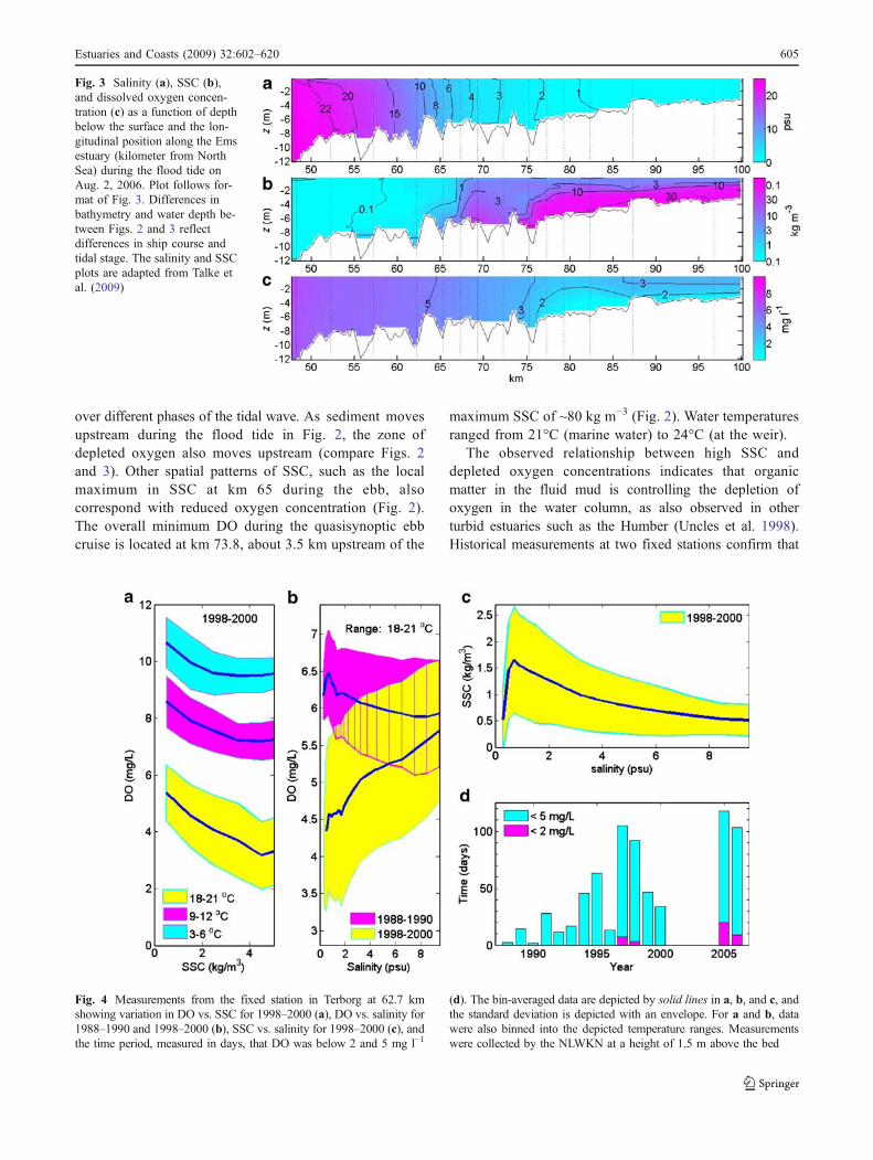
over different phases of the tidal wave. As sediment movesupstream during the flood tide in Fig. 2, the zone ofdepleted oxygen also moves upstream (compare Figs. 2and 3). Other spatial patterns of SSC, such as the localmaximum in SSC at km 65 during the ebb, alsocorrespond with reduced oxygen concentration (Fig. 2).The overall minimum DO during the quasisynoptic ebbcruise is located at km 73.8, about 3.5 km upstream of the

maximum SSC of ~80 kg m−3 (Fig. 2). Water temperaturesranged from 21°C (marine water) to 24°C (at the weir).

The observed relationship between high SSC anddepleted oxygen concentrations indicates that organicmatter in the fluid mud is controlling the depletion ofoxygen in the water column, as also observed in otherturbid estuaries such as the Humber (Uncles et al. 1998).Historical measurements at two fixed stations confirm that

Fig. 4 Measurements from the fixed station in Terborg at 62.7 kmshowing variation in DO vs. SSC for 1998–2000 (a), DO vs. salinity for1988–1990 and 1998–2000 (b), SSC vs. salinity for 1998–2000 (c), andthe time period, measured in days, that DO was below 2 and 5 mg l−1

(d). The bin-averaged data are depicted by solid lines in a, b, and c, andthe standard deviation is depicted with an envelope. For a and b, datawere also binned into the depicted temperature ranges. Measurementswere collected by the NLWKN at a height of 1.5 m above the bed

Fig. 3 Salinity (a), SSC (b),and dissolved oxygen concen-tration (c) as a function of depthbelow the surface and the lon-gitudinal position along the Emsestuary (kilometer from NorthSea) during the flood tide onAug. 2, 2006. Plot follows for-mat of Fig. 3. Differences inbathymetry and water depth be-tween Figs. 2 and 3 reflectdifferences in ship course andtidal stage. The salinity and SSCplots are adapted from Talke etal. (2009)

Estuaries and Coasts (2009) 32:602–620 605

oxygen depletion correlates well with SSC (Figs. 4 and 5).Figures 4a and 5a show envelopes of the average DO andits standard deviation as a function of SSC, with DOmeasurements separated into water temperature bins reflect-ing typical summer conditions (18–21°C), spring andautumn conditions (9–12°C) and winter conditions (0–3°C).At both locations, DO concentrations decrease approximate-ly linearly with increasing SSC (Fig. 4a) and turbidity(proportional to SSC; Fig. 5a), although the slope decreasesslightly at higher SSC. Dissolved oxygen concentrations area strong function of temperature: colder water is moreoxygenated at zero SSC and the rate of depletion as afunction of SSC is smaller. Significant variation (standarddeviation of approximately ±1 mg l−1) is found in the trendsobserved in Figs. 4a and 5a. A partial list of possible causesincludes changing aeration due to wind, variable mixing dueto tides (e.g., spring–neap), advection and diffusion fromupstream and downstream, recent conditions (e.g., conditionsover the previous time period), changes in biological factors,or other sources of DO depletion (e.g., patchiness indistribution of organic material or microorganisms). None-theless, to first order, the depletion of DO can be consideredto be proportional to SSC.

The SSC which causes DO depletion is typically trappedwithin an estuarine turbidity zone which is centered within

a band of salinity between 0.5 and 2 psu (Figs. 4c and 5c).At low salinity (<0.3 psu), which occurs during elevatedfreshwater discharge at these locations, SSC and turbiditydecrease markedly. Conversely, the salt wedge movesupstream during low discharge and the measured SSCdecreases as salinity increases (> 2 psu). Because thestation of Leer-Leda (Fig. 5) is nearly 15 km upstream ofTerborg (Fig. 4), salinity there does not exceed 2 psu.

The SSC and turbidity distribution suggest a conceptualpicture in which organic material (attached to SSC)produces a sag (minimum) in the along-estuary distributionof DO, with more oxygenated conditions observed at thefreshwater and saline boundaries of the ETZ (see alsoFigs. 2 and 3). Such a DO sag is confirmed bycontemporary measurements from 1998 to 2000, whichshows that DO concentrations increase markedly duringfreshwater conditions (Fig. 5b) and more marine conditions(Fig. 4b), with minimum DO concentrations occurring inbrackish water between 0.5 and 2 psu. Comparison withhistorical measurements from 1988 to 1990 (Fig. 4b) and1984 to 1986 (Fig. 5b) shows a downwards shift in DO inthe ETZ over time of between 1 and 3 mg l−1, on average.No significant change in DO is observed at the boundariesof the ETZ. Hence, though historical measurements of SSCare unavailable, the results indicate that the increased

Fig. 5 Measurements from the fixed station in Leer-Leda showingvariation in DO vs. turbidity for 1998–2000 (a), DO vs. salinity for 1984–1986, 1991–1993, and 1998–2000 (b), turbidity vs. salinity for 1998–2000 (c), and the time period, measured in days, that DO was below 2and 5 mg l−1 (d). The bin-averaged data are depicted by solid lines in a,

b, and c, and the standard deviation is depicted with an envelope or bars.For a and b, data were also binned into the depicted temperature ranges.Measurements were collected by the NLWKN at a height of 1 m belowthe water surface. The station is located approximately 3.9 km from thedischarge of the Leda into the Ems at 73.3 km

606 Estuaries and Coasts (2009) 32:602–620

contemporary depletion of oxygen in the ETZ is likelyoccurring because of increased SSC (and not other factors).The majority of increased oxygen demand apparently oc-curred after 1993 since mean DO concentrations in 1991–1993 are only slightly less than 1984–1986 (Fig. 5b). Thedecrease in DO concentrations (particularly after 1994)coincides with progressive deepening of the river Ems in1985–1986, 1991–1992, and 1994 from ~5 m to ~7 mbetween Emden (km 46) and Papenburg (km 87; Jensen et al.2003) and increased maintenance dredging (de Jonge 2000).

The worsening DO conditions over the past two decadesare confirmed by considering the time (measured in daysper year) that DO concentrations are below the threshold of5 and 2 mg l−1 (Figs. 4d and 5d). Whereas less than20 days/year dipped below the 5 mg l−1 threshold before1991 at either station, conditions worsen to a high of~118 days in 2005 at Terborg (data were unavailable past2000 for Leer-Leda). Hypoxic conditions (<2 mg l−1) neveroccurred at either station before 1997 but are becomingincreasingly common and are occurring for longer timeperiods (~20 days in 2005). Because DO concentrations of5 and 2 mg l−1 are thresholds below which many fish andother organisms become stressed or killed, respectively, theenvironmental quality of the river Ems has clearlydegraded.

Because the DO sag in the Ems estuary is linked to themagnitude of SSC and its longitudinal distribution, under-standing the physical factors which change the ETZ (e.g.,freshwater discharge or water depth) becomes essential forunderstanding DO dynamics. The persistence of elevatedSSC and depressed DO during both the flood and ebb(Figs. 2 and 3) suggests that a tidally averaged model cancapture the subtidal distribution of SSC and DO. Toidentify and understand the physical factors controllingoxygen depletion, we next develop an idealized model forthe distribution of SSC and DO in an estuary.

Model

The oxygen depletion model we develop for an idealizedestuary uses analytical solutions to tidally averaged circula-tion and SSCs developed by Talke et al. (2008, 2009). Here,we first outline the hydrodynamic and morphodynamicmodels (more details are available in Supplement S.1) andthen develop the DO concentration model.

Hydrodynamic and SSC Model

The tidally averaged hydrodynamic model of Talke et al.(2008, 2009) extends the classical definition of estuarinecirculation (Hansen and Rattray 1965; Officer 1976) toinclude currents that arise due to longitudinal density

gradients of SSC. The model applies the rigid-lid assump-tion, assumes no slip at the bottom boundary and no shearat the top, and assumes that eddy viscosity Av, eddydiffusivity Kv, depth H, longitudinal dispersion Kh, and thesettling velocity ws of sediment particles are constantthroughout the model domain (see Fig. 6 for a review ofkey assumptions). The x-axis points upstream and theorigin x=0 is at the seaward boundary. The z-axis pointsupwards from the water surface. Following other idealizedstudies (e.g., Friedrichs et al. 1998), we define a funnel-shaped estuary such that the development of width b withdistance is described by an exponential function,

bðxÞ ¼ Bo exp�x

Le

� �; ð1Þ

where Bo is the width at the estuary mouth (x = 0) and Le isthe convergence length scale of the estuary. Following Odd(1988), the equation of state for the model is a linearizedfunction of both salinity s(x) and suspended sedimentconcentration C(x,z):

rðx; zÞ ¼ ro þ bsðxÞ þ gCðx; zÞ: ð2Þ

In this expression, ρ(x,z) is the combined density (kg m−3);ρo (kg m−3) is the density of water; ß is ~0.83 kg m−3 psu−1

and converts salt to density and γ=(ρs−ρo)/ρs~0.62 convertsSSC into density, where ρs is the density of the sedimentparticles, here assumed to be sand for simplicity. We assumethat salinity is well mixed vertically (as suggested by Figs. 2and 3) and is described longitudinally by a hyperbolictangent (see also Warner et al. 2005):

sðxÞ ¼ 0:5So 1� tanhx� xcxL

� �� �; ð3Þ

Constant sediment oxygen demand (SOD)

Non-cohesive, finegrained sediments

Constant settling velocity

Constant eddy viscosity and diffusivity

Salinity wellmixed, prescribedlongitudinally

Exponentially decreasing width

Constant depth

<Tidally averaged>

Decay of oxygen proportional to SSC (organic matter)

Constant reaeration coefficient

Rigid lid

zx

Erosion = Deposition

Fig. 6 Assumptions made during derivation of model

Estuaries and Coasts (2009) 32:602–620 607

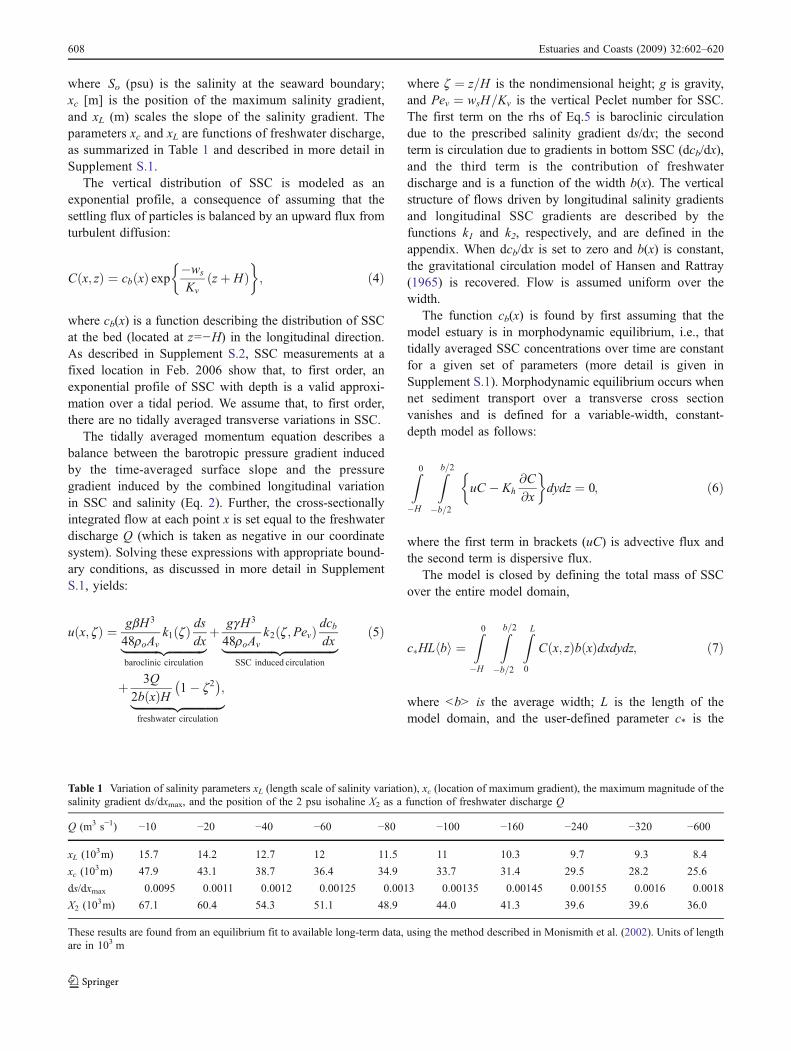
where So (psu) is the salinity at the seaward boundary;xc [m] is the position of the maximum salinity gradient,and xL (m) scales the slope of the salinity gradient. Theparameters xc and xL are functions of freshwater discharge,as summarized in Table 1 and described in more detail inSupplement S.1.

The vertical distribution of SSC is modeled as anexponential profile, a consequence of assuming that thesettling flux of particles is balanced by an upward flux fromturbulent diffusion:

Cðx; zÞ ¼ cbðxÞ exp �ws

Kvðzþ HÞ

� �; ð4Þ

where cb(x) is a function describing the distribution of SSCat the bed (located at z=−H) in the longitudinal direction.As described in Supplement S.2, SSC measurements at afixed location in Feb. 2006 show that, to first order, anexponential profile of SSC with depth is a valid approxi-mation over a tidal period. We assume that, to first order,there are no tidally averaged transverse variations in SSC.

The tidally averaged momentum equation describes abalance between the barotropic pressure gradient inducedby the time-averaged surface slope and the pressuregradient induced by the combined longitudinal variationin SSC and salinity (Eq. 2). Further, the cross-sectionallyintegrated flow at each point x is set equal to the freshwaterdischarge Q (which is taken as negative in our coordinatesystem). Solving these expressions with appropriate bound-ary conditions, as discussed in more detail in SupplementS.1, yields:

u x; zð Þ ¼ gbH3

48roAvk1 zð Þ ds

dx|fflfflfflfflfflfflfflfflfflfflfflffl{zfflfflfflfflfflfflfflfflfflfflfflffl}baroclinic circulation

þ ggH3

48roAvk2 z;Pevð Þ dcb

dx|fflfflfflfflfflfflfflfflfflfflfflfflfflfflfflfflffl{zfflfflfflfflfflfflfflfflfflfflfflfflfflfflfflfflffl}SSC induced circulation

þ 3Q

2bðxÞH 1� z2� �

;|fflfflfflfflfflfflfflfflfflfflfflfflffl{zfflfflfflfflfflfflfflfflfflfflfflfflffl}freshwater circulation

ð5Þ

where z ¼ z=H is the nondimensional height; g is gravity,and Pev ¼ wsH=Kv is the vertical Peclet number for SSC.The first term on the rhs of Eq.5 is baroclinic circulationdue to the prescribed salinity gradient ds/dx; the secondterm is circulation due to gradients in bottom SSC (dcb/dx),and the third term is the contribution of freshwaterdischarge and is a function of the width b(x). The verticalstructure of flows driven by longitudinal salinity gradientsand longitudinal SSC gradients are described by thefunctions k1 and k2, respectively, and are defined in theappendix. When dcb/dx is set to zero and b(x) is constant,the gravitational circulation model of Hansen and Rattray(1965) is recovered. Flow is assumed uniform over thewidth.

The function cb(x) is found by first assuming that themodel estuary is in morphodynamic equilibrium, i.e., thattidally averaged SSC concentrations over time are constantfor a given set of parameters (more detail is given inSupplement S.1). Morphodynamic equilibrium occurs whennet sediment transport over a transverse cross sectionvanishes and is defined for a variable-width, constant-depth model as follows:

Z0

�H

Zb=2�b=2

uC � Kh@C

@x

� �dydz ¼ 0; ð6Þ

where the first term in brackets (uC) is advective flux andthe second term is dispersive flux.

The model is closed by defining the total mass of SSCover the entire model domain,

c�HL bh i ¼Z0

�H

Zb=2�b=2

ZL0

Cðx; zÞbðxÞdxdydz; ð7Þ

where <b> is the average width; L is the length of themodel domain, and the user-defined parameter c* is the

Table 1 Variation of salinity parameters xL (length scale of salinity variation), xc (location of maximum gradient), the maximum magnitude of thesalinity gradient ds/dxmax, and the position of the 2 psu isohaline X2 as a function of freshwater discharge Q

Q (m3 s−1) −10 −20 −40 −60 −80 −100 −160 −240 −320 −600

xL (103m) 15.7 14.2 12.7 12 11.5 11 10.3 9.7 9.3 8.4

xc (103m) 47.9 43.1 38.7 36.4 34.9 33.7 31.4 29.5 28.2 25.6

ds/dxmax 0.0095 0.0011 0.0012 0.00125 0.0013 0.00135 0.00145 0.00155 0.0016 0.0018

X2 (103m) 67.1 60.4 54.3 51.1 48.9 44.0 41.3 39.6 39.6 36.0

These results are found from an equilibrium fit to available long-term data, using the method described in Monismith et al. (2002). Units of lengthare in 103 m

608 Estuaries and Coasts (2009) 32:602–620

average SSC over the model domain. For a given averageconcentration c*, the morphodynamic equilibrium (Eq. 6) issolved analytically, using Eqs. 1, 4, and 5, to define theequilibrium distribution of SSC:

C x; zð Þ ¼ A1 exp FðxÞð Þ|fflfflfflfflfflffl{zfflfflfflfflfflffl}longitudinal component

exp�ws

Kvzþ Hð Þ

� �;|fflfflfflfflfflfflfflfflfflfflfflfflfflfflfflffl{zfflfflfflfflfflfflfflfflfflfflfflfflfflfflfflffl}

vertical component

ð8aÞ

FðxÞ ¼ �TsgbH3sðxÞ48roAvTKKh|fflfflfflfflfflfflfflfflfflffl{zfflfflfflfflfflfflfflfflfflffl}

baroclinic component

� TTgH3cbðxÞ48roAvTKKh|fflfflfflfflfflfflfflfflffl{zfflfflfflfflfflfflfflfflffl}SSC component

þ 3TQQLe2HTKKHbðxÞ|fflfflfflfflfflfflfflfflfflffl{zfflfflfflfflfflfflfflfflfflffl}freshwater component

;

ð8bÞ

where TS, TQ, TT, and TK are parameters that are defined inthe “Appendix.” The longitudinal distributions of salinity,SSC, and freshwater discharge all contribute to theequilibrium distribution of sediment. The definition of c*is used to find the constant A1:

A1 ¼ c�PevL < b >

1� exp �Pevf gð Þ R L0 bðxÞ exp FðxÞf gdx

: ð9Þ

Equations 8a, 8b, and 9 are solved iteratively, asdescribed in Supplement S.1.

Oxygen Consumption by Suspended Sediment OxygenDemand

In typical rivers and estuaries, the depletion of oxygenoccurs from the consumption of organic material and isexpressed as biological oxygen demand (BOD), sedimentoxygen demand at the consolidated bed (SOD), chemicaloxygen demand, and nitrogen oxygen demand (NBOD;Cox 2003). BOD occurs on individual molecules, colloidalmaterial, and on detritus associated with suspended sedi-ment aggregates in the water column. Here, we focus onoxygen depletion due to sediment-linked biological mate-rial that is trapped at the estuarine turbidity maximum.Measurements show that the organic content of SSC in theEms ranges from 10% to 20% and consists of refractory(relatively “old”) material with a slow degradation rate and

rate of oxygen consumption (personal communication, A.Scholl; Wurpts and Torn 2005). However, because near-bottom SSCs exceed 50 kg m−3 (see Figs. 3 and 4), the totalorganic material and oxygen demand is capable ofdepleting oxygen. To gain better understanding of theeffect of elevated concentrations of organic material on DOconcentrations, we explicitly neglect the oxygen depletedby NBOD. Similarly, we neglect oxygen added by algalproduction and consumed through respiration, since highturbidity severely limits light and algal growth (Colijn1982; May et al. 2003). These processes are left for futurestudy.

To model the depletion of oxygen (O2) due to organicmaterial in the water column, we assume that the oxygenconsumption within a control volume is proportional to theconcentration of organic material, which in turn isproportional to SSC. This rate of change is modified by afactor of O2/(km+O2), where km is a constant which istypically set equal to 0.7×10−3kg m−3 (Cox 2003). Thisfactor ensures that the rate of oxygen consumption goes tozero in the limit of zero oxygen concentration. Hence, wedefine the suspended sediment oxygen demand to be

SSOD ¼ �O2

km þ O2pkrðTÞC x; zð Þ; ð10Þ

where p is the percent organic material in the SSC and is setto 0.1, and kr [s

−1] is a (positive) rate of decay of organic(carbonaceous) material that varies with temperature T. Thetemperature dependence is based on the Arrhenius relationand is commonly modeled as krðTÞ ¼ kref q

1=To T�Trefð Þ,where θ is a parameter which ranges from 1.04 to 1.13;Tref is a reference temperature of 20°C, and To=1°C is adummy variable applied to retain nondimensionality (seeCox 2003). Reported values for the organic material decaycoefficient (carbonaceous oxygen demand) at 20°C, kref,range from ~10−7s−1 to 2.3×10−5s−1 or 0.01 day−1 to2.0 day−1 (Cox 2003). We use a value of kref that is an orderof magnitude smaller (1.3 10−8 s−1), as described in“Model Calibration and Validation” (see Table 2). Tomaintain consistency in the units, we express oxygen O2

in units of kilogram per cubic meter in the model; in theresults section, we convert O2 to the more commonlyreported units of milligram per liter.

Table 2 Standard parameters prescribed in the vertical model of oxygen depletion (Model Calibration and Validation): Kv=eddy diffusivity, H=depth, ws=settling velocity, kL=aeration coefficient, Sb=bottom oxygen demand, kr=oxygen demand due to SSC, p=proportion of SSC that isorganic matter, T=water temperature

Kv (m2 s−1) H (m) ws (ms−1) kL (ms−1) Sb (kg O2 m

−2 s−1) kref (s−1) p (−) T (oC)

“Local fit” 0.001 7 0.001 10−5 5×10−8 8×10−9 0.1 20

“Estuary fit” 0.001 7 0.001 10−5 3×10−8 1.3×10−8 0.1 20

Table 2 Standard parameters prescribed in the vertical model of oxygendepletion (Model Calibration and Validation): Kv=eddy diffusivity,H=depth, ws=settling velocity, kL=aeration coefficient, Sb=bottom

oxygen demand, kr=oxygen demand due to SSC, p=proportion ofSSC that is organic matter, T=water temperature

Estuaries and Coasts (2009) 32:602–620 609

Next, we apply the control volume approach to oxygenfluxes in the model estuary, applying the assumption thathorizontal velocity u, vertical velocity w, O2, longitudinaldispersion Kh, and eddy diffusivity Kv are uniform over thewidth. The kinematic conditions for velocity are applied atthe side walls (y=± b/2), and no normal flux of oxygen isassumed through these boundaries. Assuming steady con-ditions and integrating over width, the mass balance of O2

becomes

O ¼ @

@xbuO2ð Þ � @

@zbwO2ð Þ þ @

@xbKh

@O2

@x

� �þ @

@z

� bKv@O2

@z

� �� b

O2

km þ O2pkrC:

ð11Þ

The first two terms on the right-hand side are theconvergence of width-integrated advective flux of DO; thethird and fourth terms are the convergence of width-integrated diffusive flux of DO, and the last term is thesink of DO. We simplify using the continuity equation(mass balance of water),

0 ¼ @

@xbuð Þ þ @

@zbwð Þ; ð12Þ

which yields the following equation for O2(x,z),

0¼�u@O2

@x� w

@O2

@z|fflfflfflfflfflfflfflfflfflfflfflfflffl{zfflfflfflfflfflfflfflfflfflfflfflfflffl}advection

� Kh

Le

@O2

@xþKv

@2O2

@z2þKh

@2O2

@x2|fflfflfflfflfflfflfflfflfflfflfflfflfflfflfflfflfflfflfflfflfflfflfflfflfflfflffl{zfflfflfflfflfflfflfflfflfflfflfflfflfflfflfflfflfflfflfflfflfflfflfflfflfflfflffl}diffusion

� O2

kmþO2pkrC|fflfflfflfflfflfflfflfflfflffl{zfflfflfflfflfflfflfflfflfflffl}

sink

:

ð13ÞThe vertical velocity, w, is found from continuity

(Eq. 12), using Eq. 1 and the solution from Eq. 5. Theterm � Kh

Le@O2@x arises from the transport caused by the width

convergence of the estuary; for channels (Le large), thisterm becomes negligible. Because sediment concentrationC(x,z) and the velocity u(x,z) are known by Eqs. 8a, 8b, and5, respectively, only DO concentrations are unknown andmust be solved for using the appropriate boundaryconditions. At the consolidated bed, we assume that oxygenis consumed by the SOD at the rate Sb(T) (kg O2 m

−2 s−1),

Kv@O2

@z

����z¼�H

¼ O2

km þ O2SbðTÞ

����z¼�H

: ð14Þ

In analogy with oxygen demand in the water column(Eq. 10), we model the effect of temperature asSbðTÞ ¼ Sbrq

1=To T�Trefð Þ, where Sbr is a constant at thereference temperature of 20°C, and add the corrective factorO2/(km+O2) to ensure that negative DO concentrationscannot occur. Typical river and estuary values of Sbr rangefrom ~10−9 kg O2 m

−2 s−1 (sandy or mineral bed) to 10−7 kg

O2 m−2 s−1 (organic deposits), with typical estuarine valuesof ~1 to 2×10−8 kg O2 m

−2 s−1 (Chapra 1997). In the muddySeine estuary, measurements by Garban et al. 1995 reportedan SOD value of 3.2×10−8 kg O2 m−2 s−1, with a range of1.7×10−8 kg O2 m−2 s−1 to 8.3×10−8 kg O2 m−2 s−1. Wecalibrate our model using these reported ranges of SOD in“Model Calibration and Validation.” At the surface, the fluxof oxygen between the atmosphere and the water column isproportional to the difference between saturated conditions(O2,sat) and actual conditions (O2|z=0):

Kv@O2

@z

����z¼0

¼ kL O2;sat � O2jz¼0

� �; ð15Þ

where kL (m s−1) is an empirical constant that depends onclimatic conditions, depth, and hydrodynamic conditions (see,e.g., Cox 2003). The flux of oxygen at the surface is oftenassumed to be a constant on the order of 10−8 kg O2 m

−2 s−1

(Lin et al. 2006). Here, we allow the flux to vary based onthe oxygen deficit at the surface. In the Seine River, Garnieret al. (2001) found values of the aeration coefficient kL alongdifferent reaches to be between 0 and 0.07 m h−1, withaverages between 0.02 and 0.07 m h−1 (5×10−6 m s−1 to 2×10−5 m s−1). Cox (2003) lists multiple studies with depth-averaged values of the aeration coefficient that vary between0 and 250 day−1 with an order of magnitude of ~0.4 day−1

for large rivers, or, when scaled by a depth of H=7 m,approximately 3×10−5 m s−1. The saturated oxygen concen-tration is a function of temperature and salinity and is~8.5 mg l−1 at 20°C (APHA 1992). The downstream andupstream boundary condition (x=0 and x=L) is found fromthe modeled SSC at the boundary, using the simplified 1DDO model described below. The 2D model is solved usingan implicit finite difference algorithm with 100 along-channel grid points and 30 vertical grid points.

To gain fundamental understanding of DO depletion andto obtain an upstream and downstream boundary condition,we simplify Eq. 13 by assuming that horizontal advectionand dispersion terms are negligible, to first order (i.e., terms1, 3, and 5 can be neglected). When applied as a boundarycondition, the appropriateness of this assumption must bechecked against results. Also assuming negligible verticalvelocities, the simplified 1D model requires that

0 ¼ Kvd2O2

dz2� O2

km þ O2pkrCðzÞ: ð16Þ

This equation is solved numerically using the boundaryconditions described in Eqs. 14 and 15. The verticalvariation of SSC, C(z), is prescribed by the parameter c*(Eq. 7), which in this case reduces to the depth-averagedSSC. For clarity, we denote this depth-averaged SSC by c*dand reserve c* for the estuary-averaged SSC.

610 Estuaries and Coasts (2009) 32:602–620

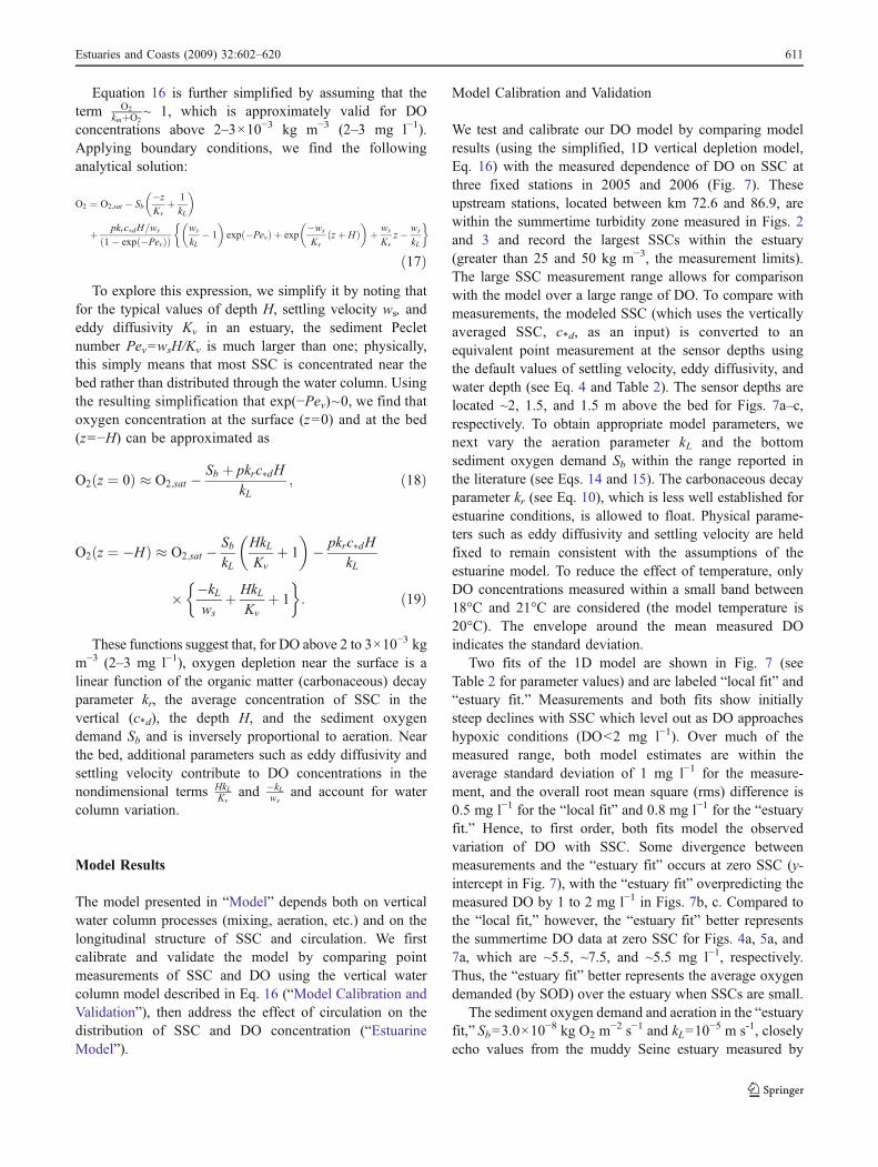
Equation 16 is further simplified by assuming that theterm O2

kmþO2~ 1, which is approximately valid for DO

concentrations above 2–3×10−3 kg m−3 (2–3 mg l−1).Applying boundary conditions, we find the followinganalytical solution:

O2 ¼ O2;sat � Sb�z

Kvþ 1

kL

� �

þ pkrc�dH=ws

1� exp �Pevð Þð Þws

kL� 1

� �exp �Pevð Þ þ exp

�ws

Kvzþ Hð Þ

� �þ ws

Kvz� ws

kL

� �

ð17ÞTo explore this expression, we simplify it by noting that

for the typical values of depth H, settling velocity ws, andeddy diffusivity Kv in an estuary, the sediment Pecletnumber Pev=wsH/Kv is much larger than one; physically,this simply means that most SSC is concentrated near thebed rather than distributed through the water column. Usingthe resulting simplification that exp(−Pev)~0, we find thatoxygen concentration at the surface (z=0) and at the bed(z=−H) can be approximated as

O2 z ¼ 0ð Þ � O2;sat � Sb þ pkrc�dHkL

; ð18Þ

O2 z ¼ �Hð Þ � O2;sat � SbkL

HkLKv

þ 1

� �� pkrc�dH

kL

� �kLws

þ HkLKv

þ 1

� �: ð19Þ

These functions suggest that, for DO above 2 to 3×10−3 kgm−3 (2–3 mg l−1), oxygen depletion near the surface is alinear function of the organic matter (carbonaceous) decayparameter kr, the average concentration of SSC in thevertical (c*d), the depth H, and the sediment oxygendemand Sb and is inversely proportional to aeration. Nearthe bed, additional parameters such as eddy diffusivity andsettling velocity contribute to DO concentrations in thenondimensional terms HkL

Kvand �kL

wsand account for water

column variation.

Model Results

The model presented in “Model” depends both on verticalwater column processes (mixing, aeration, etc.) and on thelongitudinal structure of SSC and circulation. We firstcalibrate and validate the model by comparing pointmeasurements of SSC and DO using the vertical watercolumn model described in Eq. 16 (“Model Calibration andValidation”), then address the effect of circulation on thedistribution of SSC and DO concentration (“EstuarineModel”).

Model Calibration and Validation

We test and calibrate our DO model by comparing modelresults (using the simplified, 1D vertical depletion model,Eq. 16) with the measured dependence of DO on SSC atthree fixed stations in 2005 and 2006 (Fig. 7). Theseupstream stations, located between km 72.6 and 86.9, arewithin the summertime turbidity zone measured in Figs. 2and 3 and record the largest SSCs within the estuary(greater than 25 and 50 kg m−3, the measurement limits).The large SSC measurement range allows for comparisonwith the model over a large range of DO. To compare withmeasurements, the modeled SSC (which uses the verticallyaveraged SSC, c*d, as an input) is converted to anequivalent point measurement at the sensor depths usingthe default values of settling velocity, eddy diffusivity, andwater depth (see Eq. 4 and Table 2). The sensor depths arelocated ~2, 1.5, and 1.5 m above the bed for Figs. 7a–c,respectively. To obtain appropriate model parameters, wenext vary the aeration parameter kL and the bottomsediment oxygen demand Sb within the range reported inthe literature (see Eqs. 14 and 15). The carbonaceous decayparameter kr (see Eq. 10), which is less well established forestuarine conditions, is allowed to float. Physical parame-ters such as eddy diffusivity and settling velocity are heldfixed to remain consistent with the assumptions of theestuarine model. To reduce the effect of temperature, onlyDO concentrations measured within a small band between18°C and 21°C are considered (the model temperature is20°C). The envelope around the mean measured DOindicates the standard deviation.

Two fits of the 1D model are shown in Fig. 7 (seeTable 2 for parameter values) and are labeled “local fit” and“estuary fit.” Measurements and both fits show initiallysteep declines with SSC which level out as DO approacheshypoxic conditions (DO<2 mg l−1). Over much of themeasured range, both model estimates are within theaverage standard deviation of 1 mg l−1 for the measure-ment, and the overall root mean square (rms) difference is0.5 mg l−1 for the “local fit” and 0.8 mg l−1 for the “estuaryfit.” Hence, to first order, both fits model the observedvariation of DO with SSC. Some divergence betweenmeasurements and the “estuary fit” occurs at zero SSC (y-intercept in Fig. 7), with the “estuary fit” overpredicting themeasured DO by 1 to 2 mg l−1 in Figs. 7b, c. Compared tothe “local fit,” however, the “estuary fit” better representsthe summertime DO data at zero SSC for Figs. 4a, 5a, and7a, which are ~5.5, ~7.5, and ~5.5 mg l−1, respectively.Thus, the “estuary fit” better represents the average oxygendemanded (by SOD) over the estuary when SSCs are small.

The sediment oxygen demand and aeration in the “estuaryfit,” Sb=3.0×10

−8 kg O2 m−2 s−1 and kL=10

−5 m s-1, closelyecho values from the muddy Seine estuary measured by

Estuaries and Coasts (2009) 32:602–620 611

Garban et al. (1995; mean Sb=3.2×10−8 kg O2 m

−2 s−1) andGarnier et al. (2001) (5×10−6 m s−1<kL<2×10

−5 m s−1).Both estimates of the organic material decay rate are anorder of magnitude smaller than reported values ofcarbonaceous decay (10−7s−1 Cox 2003) and confirm that

the organic material attached to SSC is extremely refractory(see also van Es et al. 1980; Baretta and Ruardij 1988).

The simplified analytical solutions of DO (Eqs. 18 and19) help explain differences between the measurement sitesand models. During clear conditions (zero SSC), the

Fig. 8 Variation in measuredDO as a function of tempera-ture, compared with 1D modelresults. A scatter plot ofmeasurements shows total vari-ation of data from 2005 to 2006.Saturated conditions are shownby a solid black line. “Low-SSC” and “high-SSC” measure-ments correspond to average DOfrom SSC bins of 0–1 and18–25 kg m−3, respectively.“Low-SSC model” and “high-SSC model” correspond to amodeled SSC of 0.5 and20 kg m−3 at the measurementheights of 2, 1.5, and 1.5 m for a,b, and c, respectively. Theparameters corresponding to thelocal fit to the turbid zone wereused, and a temperature adjust-ment coefficient of θ=1.1 wasused

Fig. 7 Measured average DO asa function of measured SSC atthree stations along the Ems forthe temperature range 18°C to21°C for data from 2005 to2006, compared with 1D modelresults. The standard deviationof the measurement is shown bythe envelope around the mean.Two-parameter fits are depicted:a “local” fit that minimizes errorin Weener (b) and Leerort (c),and an “estuary fit” that betterrepresents average DO over theestuary in the limit of zero SSC

612 Estuaries and Coasts (2009) 32:602–620

oxygen depletion is set by a balance between SOD andaeration, i.e., Sb/kL (see Eq. 18). Hence, the measurementsites in Figs. 7b, c may have less aeration, or greater SOD,than the site in Fig. 7a. Similarly, the slope of DO versusSSC is set by the ratio of organic material decay to aeration,i.e., kr/kL (see Eq. 18). Hence, the sites in Fig. 7b, c, whichhave slightly less slopes of DO vs SSC than Fig. 7a, may beexposed to more refractory material (higher kr) or reducedaeration. By contrast, the DO depletion slope in Terborg,km 62.7, is greater than those shown in Fig. 7 (see Fig. 4a)and suggests reduced aeration or higher degradation rates oforganic material. These considerations show that theassumption of constant conditions may oversimplify theestuarine model. However, bathymetry, tidal mixing andtransport, lateral circulation, and other factors may alsoaffect the measured DO and SSC concentrations, and it isbeyond the scope of this contribution to fully consider thesefactors. Nonetheless, the fit of the model to measurementdata (Fig. 7) confirms that that the constant parameter valuesreasonably model the bulk oxygen depletion occurring dueto SOD and SSC over a large portion of the turbid zone.

The skill of the model in predicting oxygen depletion asa function of temperature is presented in Fig. 8 for both lowSSCs (0–1 kg m−3) and elevated SSCs (18–25 kg m−3) atthree locations (Papenburg, km 86.9; Weener, km 80.1; andLeerort, km 72.6). The measured DO at both low and highSSC is binned into 2°C intervals, and the average iscompared against modeled results. The “local fit” to theETZ is used for the model (see Table 2), and the averageSSC over the water column, c*d, is adjusted to produce anSSC of 20 kg m−3 at the measurement heights. We find thatthe parameter θ, used to adjust the DO depletion rates krand Sb as a function of temperature (see Eqs. 10 and 14),best reproduces measured results with a value of θ~1.1.

Overall, the measured and modeled variation of DO withtemperature agrees to within an rms difference of ~1 mg l−1,with both depicting a nearly linear increase in DO as waterbecomes colder (Fig. 8). Moreover, the model results movecloser to saturated conditions as temperature falls andoxygen demand decreases, reflecting the same observationin the measured data. Elevated SSC conditions, labeled“high SSC,” are typically ~1–3 mg l−1 less than low-SSC

conditions in both model and measurements, though somescatter occurs in the data. During warmer (summertime)conditions, DO concentrations approach zero and theobserved variation with temperature asymptotes in boththe modeled and measured results. Model and measure-ments of high SSC do not agree well below T=19°C inPapenburg (Fig. 8a), perhaps because of a paucity of high-SSC data at lower temperatures. In Leerort (Fig. 8c),modeled DO slightly overpredicts measurements for low-SSC conditions. Besides the processes discussed for Fig. 7,other sources of variation between the model and measure-ments include variations in decay rates not captured by θand the supersaturated DO conditions that are observed tooccur periodically at low SSC. Overall, however, the bulkcharacteristics of the measured and modeled temperaturevariation agree and further validate the DO model.

Estuarine Model

Next, we analyze the patterns of circulation, SSC, and DOconcentrations that result in a model 2D estuary fromchanging freshwater discharge, depth, and mixing. Unlessotherwise stated, all parameters are held to the “estuary fit”parameters displayed in Tables 2 and 3 (SSC modelparameters). The hydrodynamic variables in Table 3 repre-sent low-freshwater-discharge conditions that occur duringthe summer months in the Ems estuary (see Talke et al.2009 for discussion). Parameter studies of settling velocity,horizontal dispersion, width variation, total sedimentsupply, and longitudinal salinity structure are described inSupplement S.3.

Figure 9 shows examples of circulation, SSC, and DOconcentrations that occur when standard parameters areused (Fig. 9b, d, f) and when one parameter, depth, isreduced from H=7 m to H=5 m (Fig. 9a, c, e). The modelestimates for SSC and DO in the H=7 m case (standardparameters) qualitatively reproduce the field conditionsobserved in Figs. 2 and 3. In both model and measurements,near-bed SSCs with magnitudes greater than 10 kg m−3

cover the bottom to depths of 1 to 2 m from the saltwedge to the tidal weir at km 100 and produce a zone ofdepleted DO that coincides with elevated SSC. The

Table 3 Standard parameters used to calculate circulation and the equilibrium distribution of sediment in the 2D model

So (psu) xL (m) xc (m) Av (m2 s−1) L (m) Q (m3 s−1) Kh (m

2 s−1) c* (kg m−3) Le (m) Bo (m)

30 14×103 43×103 0.001 100×103 −10 100 0.5 20×103 8×103

The standard depth H, settling velocity ws, and eddy diffusivity Kv are described in Table 2, as are the additional parameters needed for the oxygenmodel—kL, kr, p, and Sb. Here, S* is the salinity at the seaward boundary; xL scales the salinity gradient; xc is the location of the maximum salinitygradient relative to the seaward boundary, Av=eddy viscosity, L=length of model domain, Q=freshwater discharge, Kh=horizontal dispersioncoefficient, c* is the average SSC over the estuary; Le is the convergence length scale; and Bo is the width at the estuarine mouth. Note thatdischarge Q is negative in our coordinate system

Estuaries and Coasts (2009) 32:602–620 613

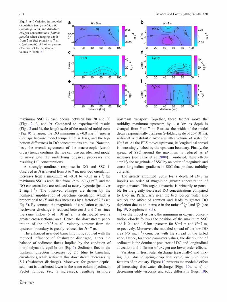
maximum SSC in each occurs between km 70 and 80(Figs. 2, 3, and 9). Compared to experimental results(Figs. 2 and 3), the length scale of the modeled turbid zone(Fig. 9) is larger; the DO minimum is ~0.8 mg l−1 greater(perhaps because model temperature is less), and the top-bottom differences in DO concentrations are less. Nonethe-less, the overall agreement of the macroscopic (zerothorder) trends confirms that we can use our idealized modelto investigate the underlying physical processes andresulting DO concentrations.

A strongly nonlinear response in DO and SSC isobserved as H is altered from 5 to 7 m; near-bed circulationincreases from a maximum of ~0.01 to ~0.03 m s−1; themaximum SSC is amplified from ~9 to ~60 kg m−3, and theDO concentrations are reduced to nearly hypoxic (just over2 mg l−1). The observed changes are driven by thenonlinear amplification of baroclinic circulation, which isproportional to H3 and thus increases by a factor of 2.5 (seeEq. 5). By contrast, the magnitude of circulation caused byfreshwater discharge is reduced between 5 and 7 m sincethe same inflow Q of −10 m3 s−1 is distributed over agreater cross-sectional area. Hence, the downstream pene-tration of the −0.05-m s−1 velocity contour from theupstream boundary is greatly reduced for H=7 m.

The enhanced near-bed baroclinic flow, coupled with thereduced influence of freshwater discharge, alters thebalance of sediment fluxes implied by the condition ofmorphodynamic equilibrium (Eq. 6). Sediment flux in theupstream direction increases by 2.5 (due to barocliniccirculation), while sediment flux downstream decreases by5/7 (freshwater discharge). Moreover, for greater depths,sediment is distributed lower in the water column (sedimentPeclet number, Pev, is increased), resulting in more

upstream transport. Together, these factors move theturbidity maximum upstream by ~10 km as depth ischanged from 5 to 7 m. Because the width of the modeldecays exponentially upstream (e-folding scale of 20×103m),sediment is distributed over a smaller volume of water forH=7 m. As the ETZ moves upstream, its longitudinal spreadis increasingly halted by the upstream boundary. Finally, thespread of SSC around the maximum is reduced as Hincreases (see Talke et al. 2008). Combined, these effectsamplify the magnitude of SSC by an order of magnitude andcause longitudinal gradients in SSC that produce turbiditycurrents.

The greatly amplified SSCs for a depth of H=7 mimplies an order of magnitude greater concentration oforganic matter. This organic material is primarily responsi-ble for the greatly decreased DO concentrations comparedto H=5 m. Particularly near the bed, deeper water alsoreduces the affect of aeration and leads to greater DOdepletion due to an increase in the ratios pkrc�dH

kLand HkL

Kv(see

Eq. 19, Supplement S.3).For the model estuary, the minimum in oxygen concen-

tration closely follows the position of the maximum SSCand is 0.4 and 1.5 km upstream for H=5 m and H=7 m,respectively. Moreover, the modeled spread of the low DOarea (<5 mg l−1) coincides with the spread of the turbidzone. Hence, for these parameter values, the distribution ofsediment is the dominant predictor of DO and longitudinaladvection and diffusion of oxygen are lower-order effects.

Variation in freshwater discharge (seasonally) and mix-ing (e.g., due to spring–neap tidal cycle) are ubiquitousfeatures of an estuary. Figure 10 presents the modeled effectof increasing freshwater discharge (Figs. 10a, c, e) ordecreasing eddy viscosity and eddy diffusivity (Figs. 10b,

Fig. 9 a–f Variation in modeledcirculation (top panels), SSC(middle panels), and dissolvedoxygen concentrations (bottompanels) when changing depthfrom 5 m (left panels) to 7 m(right panels). All other param-eters are set to the standardvalues in Table 2

614 Estuaries and Coasts (2009) 32:602–620

d, f) from standard conditions (Fig. 9b, d, f). Increasedfreshwater discharge directly increases the downstreamflow, particularly near the tidal weir where the width b issmall. In addition, the salinity field moves and its gradientbecomes steeper, leading to a greater baroclinic circulationcell that is shifted downstream by ~17 km (Table 1;Supplement S.2). These circulation changes move theETZ downstream, decrease the longitudinal spread of

SSC, and decrease the magnitude of SSC (due to largerwidth b). Increased DO concentrations result in a smallerDO sag (in the longitudinal direction) that is shifteddownstream with the ETZ.

Reducing eddy viscosity (Av) increases baroclinic circu-lation (see Eq. 5), while decreasing eddy diffusivity (Kv=Av) causes sediment to accumulate closer to the bed(Fig. 10). Together, the resulting increase in near-bed

Fig. 10 Variation in modeledcirculation (top panels), SSC(middle panels), and oxygenconcentrations (bottom panels)for a discharge of 160 m3 s−1 (a,c, e) and an eddy viscosity andeddy diffusivity of 0.0005 m2 s−1

(b, d, f). All other parameters areset to the standard values inTable 2

Fig. 11 Sensitivity in the mod-eled longitudinal profile of bot-tom (z=−H) DO concentrationto prescribed variations in sedi-ment oxygen demand Sb (a),suspended sediment oxygen de-mand kr (b), aeration kL (c), andtemperature T (d). The SSCprofile for each case found usedthe standard parameters inTable 2. The solution using thestandard DO parameters inTable 1 is given by the solidmagenta (dark shaded) profilein a, b, and c

Estuaries and Coasts (2009) 32:602–620 615

sediment flux (term uC in Eq. 6) moves suspendedsediment closer to the boundary, where smaller width andreduced longitudinal spread (due to the upstream boundary)amplify SSCs. These patterns result in greater DO depletionand an upstream movement in the DO minimum. As withthe other results (see also supplement S.3), the longitudinalvariation in DO is set primarily by the longitudinalvariation in SSC; without SSC variation, DO in Eq. 13 isprimarily set by a vertical (1D) balance.

A final sensitivity study (Fig. 11) shows changes to thelongitudinal distribution of bottom DO (z=−H) as param-eters associated only with the oxygen model (i.e., Sb, kL, kr,and T) are varied. In each case, the tidally averagedcirculation and equilibrium distribution of SSC resultingfrom Table 3 default conditions and displayed in Fig. 9b, d,respectively, are used. For Sb, kL, and T, the range of valuesin Fig. 11 reflects the reported range of each parameter (see“Oxygen Consumption by Suspended Sediment OxygenDemand”). For the refractory decay coefficient of organicmaterial, kr, we test the response of a factor of ~2.5 changein either direction.

Increasing bed demand Sb (Fig. 11a), organic materialdecay coefficient kr (Fig. 11b), and temperature T (Fig. 11d)results in increased oxygen depletion throughout the modelestuary, while increasing aeration kL (Fig. 11c) producesmore oxygenated conditions (note that increasing T raisesSb and kr simultaneously). The position of the DOminimum changes by several kilometers between differentcases, indicating the nonnegligible—but second order—affect of advection and horizontal diffusion. An approxi-mately linear response to changing conditions is observedfor aeration above 2 to 3 mg l−1, as suggested by thesimplified analytical expression (Eqs. 18 and 19): triplingthe standard aeration coefficient results in a threefoldincrease in minimum DO. Decreasing bed demand Sb to10−9 kg O2 m−2 s−1 approximately doubles the minimumDO concentration (Fig 11a). The less than proportionalresponse occurs because organic material in the watercolumn (given by kr) continues to deplete oxygen. Asimilar behavior is observed for decreasing kr (Fig. 11b).

However, the longitudinal extent of stressed (<5 mg l−1)and hypoxic DO conditions responds nonlinearly tochanges in the parameters. For example, halving theaeration coefficient from the standard condition produceshypoxic conditions over ~25 km, while tripling aerationremoves the stressed area completely (Fig. 11c). Increasingtemperature decreases the saturation DO concentration andmagnifies both Sb and kr; hence, a doubling of temperaturefrom 12°C to 25°C shifts the system from well oxygenatedto hypoxic. The modeled range of T mirrors seasonalchanges observed in the river Ems (as low as 0–1°C inwinter and 20–25°C in summer) and helps explain whyhypoxia occurs primarily in the summer months.

Discussion

The model we present differs from other models of oxygendepletion in that we consider the depletion of oxygen froma spatially variable SSC. Other models, for example Lin etal. (2006), investigate how gravitational circulation andriver discharge affect estuarine residence time and stratifi-cation and therefore the vertical profile of oxygen. In theseenvironments, the mechanism of oxygen depletion is thedecay of algae (and is thus eutrophication-driven) and aconstant sediment oxygen demand. Hence, the interactionof nutrients and algae and their residence time controlsoxygen depletion.

In highly turbid estuaries, such as the Ems, enormousamounts of SSC are trapped in the ETZ (Figs. 2, 3, 4, and5). In this situation, a dominant control on the depletion ofoxygen becomes the magnitude and distribution of organicmatter that is attached to SSCs. This oxygen demand fromorganic material is neither confined to the bed (as aboundary condition) nor spatially constant over the estuary.A minimum of DO occurs near the turbidity maximum,which is formed when the vertically integrated fluxes ofsediment from gravitational circulation and freshwaterdischarge balance each other. The convergence of thesesediment fluxes is balanced by counter-gradient fluxescaused by turbidity currents and longitudinal dispersion (i.e., fluxes proportional to dcb/dx; see Eqs. 5 and 6). Changesto the physical parameters that control these fluxes (e.g.,salinity field, freshwater discharge, sediment supply, depth,mixing, etc.) produce a new distribution of SSC and adifferent spatial variation in oxygen demand and DO.Hence, the factors which alter SSC distribution drivechanges to DO rather than the input of nutrients or theresidence time of water.

Qualitatively, the model results explain the plummet inDO concentrations since deepening the Ems estuary from5 to 7 m between 1985 and 1994. The H3 dependence ofgravitational circulation produces an inherently nonlinearresponse in SSC transport, which is amplified further bythe depth dependence of the area-averaged freshwaterdischarge and the vertical distribution of SSC. Together,these physical processes cause an order of magnitudeincrease in SSC and produce a large zone of depleted DOfor an increase from 5 to 7 m (Fig. 9). Additional factorsdriving DO downwards include the likely decrease ineddy diffusivity and eddy viscosity that occurs due tosediment-induced stratification (e.g., Munk and Anderson1948). Other variations in mixing—such as the spring–neap cycle—likely drive changes to the ETZ and low DOzone.

Seasonal variation in estuarine DO is driven both byhydrology and water temperature. Depleted DO concen-trations occur during the summer months because of low

616 Estuaries and Coasts (2009) 32:602–620

freshwater discharge (which moves the turbidity maximumupstream and amplifies SSC) and elevated temperature(which lowers DO saturation and increases decay rates ofsuspended organic matter and SOD). By contrast, greaterdischarge—which occurs during storm events in the winter—decreases SSC and organic matter concentrations bymoving the ETZ downstream (van Beusekom and de Jonge1998; Fig. 10). These conditions combine together withlower temperatures to produce an oxygenated water columnin winter.

In ecological terms, the impact of a hypoxic zone ismeasured by the area of a water body that dips below abiologically critical threshold such as 5 or 2 mg l−1. Sincethe modeled oxygen depletion depends on SSC distribution,this equivalently reduces to the length scale for which SSCis above a certain threshold. The idealized model suggeststhat the length scale depends upon the total amount ofsediment available for resuspension, the position of theturbidity maximum, and the relative spread of SSC from themaximum (see also Supplement S.3). Changes to organicdecay rates, reaeration, and temperature also affect the sizeof a depleted oxygen zone and combine together with theSSC distribution to make the system sensitive to relativelysmall changes in its parameters.

The idealized model we present for the depletion ofoxygen makes simplifying assumptions about both physicaland biological processes in order to understand, at a processlevel, the important factors that affect DO depletion fromsuspended organic matter. The tidally averaged model ofcirculation and SSC distribution neglect tidally varyingprocesses (e.g., settling lag, periodic salinity stratification,etc.) that influence circulation and the fluxes of sediment inan estuary. Our assumption of constant eddy diffusivitypossibly overestimates vertical mixing of DO, particularlyin the fluid mud layer, though field results suggest that top-bottom variation is small and generally less than 2 mg l−1.Depth and bathymetry effects are likely important, partic-ularly in the less uniform outer estuary. In the oxygen massbalance, we make the further simplifying assumption thatmodel parameters such as the aeration coefficient, theorganic matter decay coefficient, and the sediment oxygendemand are constant. In a real estuary, input of organicmatter from the rivers and ocean likely cause variation inthe decay coefficient, as do phytoplankton detritus, zoo-plankton detritus, remains of vascular plants, peat, andother sources of carbon. Measurements in the Ems showthat organic material is ~10% of the SSC for most of theturbid zone, except near the weir where organic material is~20% of SSC and has a larger rate of decay (A. Scholl,personal communication). Greater concentrations of lessrefractory material near the weir may explain the diver-gence between modeled and measured results near the weir(compare Figs. 2 and 9).

The model assumes that concentrations of algae andother input material are small compared to the mass oforganic material trapped at the turbidity maximum andcontribute negligibly to oxygen demand. Given the lightlimitation in highly turbid waters, phytoplankton produc-tion is significant only when SSC is low and is thus awayfrom our zone of interest (e.g., the outer estuary). Similarly,aeration caused by primary production is neglected sincethe available algae contribute primarily to respiration. Forsimplicity, the effect of the reduction and oxidation ofchemical compounds (e.g., Fe, Mn, and nutrient com-pounds) and neutrally buoyant colloidal matter on oxygendepletion are also not considered. A complete model ofoxygen depletion must include these additional terms andvary them in time and space; however, we explicitly restrictthe parameter complexity in order to gain insight into thefundamental effect of sediment dynamics on DO. Theoverall good qualitative agreement between measurementsand the model validates this approach.

Conclusions

Measurements in the Ems estuary show that near-bed SSCsexceeding 50 kg m−3 coincide with stressed (<5 mg l−1) andhypoxic (<2 mg l−1) DO concentrations. To a first orderapproximation, the oxygen depletion is proportional toSSC, with the depletion rate decreasing as temperature fallsor as anoxic conditions are approached. The zone ofdepleted oxygen occurs in the estuarine turbidity zone(salinity range of 0.5–2 psu), which moves as freshwaterdischarge changes. Over the past two decades, the durationof stressed conditions during summer has increased from 10to 20 days to more than 100 days, likely from increasedSSCs.

The physical and biological processes that contribute tooxygen depletion in turbid estuaries are investigated withan idealized model that simplifies estuarine geometry andbathymetry and uses tidally averaged governing equationsto investigate first-order effects. The depletion rate of DO isassumed to be proportional to SSC, and model calibrationto the data shows that the decay rate is extremely refractory.Aeration at the surface provides a source of oxygen, while aprescribed oxygen demand at the bed depletes oxygen.Within the model domain, DO is found by numericallysolving an advection–diffusion equation with a sink term,with analytical solutions used for velocity and SSC inputs.At the upstream and downstream model boundaries, DO isapproximated by using a 1D vertical water column modelwhich assumes that horizontal flux terms are negligible.

The modeled depletion of oxygen in the water column isprimarily a balance between aeration and the oxygendemand from both the bed (SOD) and suspended sediment.

Estuaries and Coasts (2009) 32:602–620 617

Horizontal advection and diffusion are second-order effectsthat modify, but do not control, the distribution of DO.Above 2 to 3 mg l−1, the oxygen depletion near the surfaceincreases approximately linearly with increases in thedepth-averaged SSC, depth, organic material decay coeffi-cient, and SOD. Near-bed DO concentrations are less thanat the surface and are further reduced by increasing depth orreducing mixing, which hinders the transmission of surfaceaeration.

Over the estuary, increases in near-bed upstream-directed currents move the ETZ upstream and amplifySSC and oxygen demand, primarily because suspendedsediment is distributed over a smaller volume of water.Hence, the nonlinear dependency of baroclinic circulationon H3, coupled with the H−1 dependence of currents fromfreshwater discharge, results in a nonlinear DO responseas depth is changed. Variations in the longitudinal spreadof SSC around the maximum, which are set by hydrody-namic parameters, also affect oxygen demand. Increasingthe relative amount of SSC near the bed (by increasingPev=wsH/Kv) both amplifies the effect of near-bedupstream currents and alters the distribution of SSC.Therefore, the coupled effect of mixing (Av and Kv) onboth circulation and vertical SSC distribution produces anonlinear DO response. Hence, for a turbid estuary, adominant control on oxygen depletion is the SSCdynamics, rather than the residence time of water ornutrient inputs.

Both model results and field measurements show astrong seasonal variation in DO concentrations that arecaused both by temperature-induced variation in the decayrates of organic material (i.e., changing kr and Sb) andoxygen saturation and by variation in the hydrologic cyclewhich typically produces low discharge—and high organicmaterial concentrations—during the summer months. Thisseasonal cycle has been altered by deepening the river Emsfrom 5 to 7 m, which has moved the ETZ upstream andamplified SSC. Thus, anthropogenically driven changes tothe sediment dynamics explain the reduction in averagesummertime DO by as much as 2 to 3 mg l−1 over the pastseveral decades and the much greater occurrence ofhypoxic events.

Acknowledgments Many thanks toVerena Brauer, Robbert Schippers,Karin Huijts, Marcel van Maarseveen, and Frans Buschman for logisticalsupport during experiments. Thanks also to Martin Krebs and HelgeJuergens fromWSAEmden, RewertWurpts, UweBoekhoff, and BaerbelAmman from Niedersachsen Ports (NP), Andreas Engels from NLWKN,and Christine Habermann from the Bundesanstalt fuer Gewaesserkunde(BfG). Andreas Scholl of BfG is especially thanked for his extensivepersonal communication. The crews of the Delphin (NP) and the WSAFriesland are also thanked. This work was funded by LOICZ project014.27.013 (Land Ocean Interaction in the Coastal Zone), and adminis-tered by NWO-ALW, the Netherlands Organization for ScientificResearch.

Appendix

The functions k1 and k2 produce the vertical structure ofcurrents driven by salinity gradients and turbidity gradients,respectively (Eq.5), and depend on the vertical coordinateand the sediment Peclet number Pev=wsH/Kv.

k1 zð Þ ¼ 1� 9z2 � 8z3� �

; ð20Þ

k2 z;Pevð Þ ¼ 12G1Pe�4v exp �Pev 1þ zð Þð Þ; ð21Þ

where G1 is defined as

G1 ¼ 4Pev þ 6 �1þ 13 Pev þ z2 � Pevz

2� �

exp Pev 1þ zð Þð Þþ 1þ zð Þ exp Pevzð Þ 6� 6z þ 1þ 3zð ÞPe2v

:

ð22Þ

The expressions Ts, Tt, TQ, and TK in Eqs. 13, 14, and 15are defined as follows:

TS ¼Z 0

�1k1 zð Þ exp �Pev z þ 1ð Þð Þdz; ð23Þ

TT ¼Z 0

�11� z2� �

exp �Pev z þ 1ð Þð Þdz; ð24Þ

TQ ¼Z 0

�1k2 z;Pevð Þ exp �Pev z þ 1ð Þð Þdz; ð25Þ

TKh ¼Z 0

�1exp � z þ 1ð ÞPevð Þdz: ð26Þ

By solving, these expressions reduce to functions of thesediment Peclet number Pev:

TS¼ 1

Pe4v�48þ Pe3v � 18Pev� �

exp �Pevð Þþ48� 30Pev þ 6Pe2v

;

ð27Þ

TT ¼ 144G2Pe�7v exp �2Pevð Þ; ð28Þ

G2¼�1þ 112 Pe

4vþ Pe2vþ 1

2 Pe3vþ �2Pev � Pe2v þ 1

3 Pe3v þ 2

� �exp Pevð Þþ �1� Pe2v þ 1

6 Pe3v þ 2Pev

� �exp 2Pevð Þ;

ð29Þ

TQ ¼ �2

Pe3v1� Pev þ �1þ 1

2Pe2v

� �exp �Pevð Þ

� �; ð30Þ

TKh ¼1� exp �Pevð Þ

Pev: ð31Þ

618 Estuaries and Coasts (2009) 32:602–620

References

APHA. 1992. Standard methods for the examination of water andwastewater, 18th ed. Washington, DC: American Public HealthAssociation, American Waterworks Association, Water Environ-ment Federation.

Baretta, J.W. and P. Ruardij (eds). 1988. Tidal flat estuaries:Simulation and analysis of the Ems estuary. Ecological studies,vol. 71, 353. Heidelberg: Springer.

Benoit, P., Y. Gratton, and A. Mucci. 2006. Modeling of dissolvedoxygen levels in the bottom waters of the Lower St. Lawrenceestuary: Coupling of benthic and pelagic processes. MarineChemistry 102: 13–32. doi:10.1016/j.marchem. 2005.09.015.

Borsuk, M.E., C.A. Stow, R.A. Luettich Jr., H.W. Paerl, and J.L.Pinckney. 2001. Modelling oxygen dynamics in an intermittentlystratified estuary: Estimation of process rates using field data.Estuarine, Coastal and Shelf Science 52: 33–49.

Chapra, S.C. 1997. Surface water-quality modeling. New York:McGraw-Hill.

Colijn, F. 1982. Light absorption in the waters of the Ems–Dollardestuary and its consequences for the growth of phytoplankton andmicrophytobenthos. Netherlands Journal of Sea Research 15:196–216.

Cox, B.A. 2003. A review of dissolved oxygen modeling techniquesfor lowland rivers. The Science of the Total Environment 314–316: 303–334. doi:10.1016/S0048-9697(03)00062-7.

Dai, M., X. Guo, W. Zhai, L. Yuan, B. Wang, L. Wang, P. Cai, T.Tang, and W.J. Cai. 2006. Oxygen depletion in the upper reach ofthe Pearl River estuary during a winter drought. MarineChemistry 102: 159–169. doi:10.1016/j.marchem.2005.09.020.

de Jonge, V.N. 2000. Importance of temporal and spatial scales inapplying biological and physical process knowledge in coastalmanagement, an example for the Ems estuary. Continental ShelfResearch 20: 1655–1686.

de Jonge, V.N. and L.A. Villerius. 1989. Possible role of carbonatedissolution in estuarine phosphate dynamics. Limnology andOceanography 34: 332–340.

Diaz, R.J. and R. Rosenberg. 1995. Marine benthic hypoxia: A reviewof its ecological effects and the behavioral responses of benthicmacrofauna. Oceanography and marine and biology: An annualreview 33: 245–303.

Engle, V.D., J.K. Summers, and J.M. Macauley. 1999. Dissolvedoxygen conditions in northern Gulf of Mexico estuaries.Environmental Monitoring and Assessment 57: 1–20.

Essink, K. 2003. Response of an estuarine ecosystem to reducedorganic waste discharge. Aquatic Ecology 37(1): 65–76.

Fang, T.H. and C.L. Lin. 2002. Dissolved and particulate trace metalsand their partitioning in a hypoxic estuary: The Tanshui Estuaryin northern Taiwan. Estuaries 25: 598–607.

Friedrichs, C.T., B.D. Armbrust, and H.E. de Swart. 1998. Hydrody-namics and equilibrium sediment dynamics of shallow, funnel-shaped tidal estuaries. In Physics of estuaries and coastal seas,ed. J. Dronkers and M.B.A.M. Scheffers, 315–327. Rotterdam:Balkema.

Garban, B., D. Olivon, M. Poulin, V. Gaultier, and A. Chesterikoff.1995. Exchanges at the sediment–water interface in the riverSeine, downstream from Paris. Water Research 29: 473–481.

Garnier, J., P. Servais, G. Billen, M. Akopian, and N. Brion. 2001.Lower Seine River and estuary (France) carbon and oxygenbudgets during low flow. Estuaries 24: 964–976.

Hagy, J.D. and M.C. Murrell. 2007. Susceptibility of a northern Gulfof Mexico estuary to hypoxia: An analysis using box models.Estuarine, Coastal and Shelf Science 74: 239–253. doi:10.1016/j.ecss.2007.04.013.

Hagy III, J.D., W.R. Boyton, C.W. Keefe, and K.V. Wood. 2004.Hypoxia in Chesapeake Bay, 1950–2001: Long-term change inrelation to nutrient loading and river flow. Estuaries 27: 634–658.

Hansen, D.V. and M. Rattray Jr. 1965. Gravitational circulation instraits and estuaries. Journal of Marine Research 23: 104–122.

Helder, W. and P. Ruardij. 1982. A one-dimensional mixing andflushing model of the Ems–Dollart estuary: calculation of timescales at different river discharges. Netherlands Journal of SeaResearch 15: 293–312.

Jensen, J., C. H. Mudersbach, and C. Blasi. 2003. Hydrologicalchanges in tidal estuaries due to natural and anthropogeniceffects. In Proceedings of the 6th International MEDCOAST2003 Conference, Ravenna, Italy.

Kineke, G.C. and R.W. Sternberg. 1992. Measurements of high-concentration suspended sediments using the optical backscattersensor. Marine Geology 108: 253–258.

Krebs, M., and H. Weilbeer, 2008. Ems Dollart estuary. Die Küste 74.Lin, J., L. Xie, L.J. Pietrafesa, J. Shen, M.A. Mallin, and M.J. Durako.

2006. Dissolved oxygen stratification in two micro-tidalpartially-mixed estuaries. Estuarine, Coastal and Shelf Science70: 423–437. doi:10.1016/j.ecss.2006.06.032.

Lung, W.S. and A.J. Nice. 2007. Eutrophication model for thePatuxent estuary: Advances in predictive capabilities. Journalof Environmental Engineering 133: 917–930. doi:10.1061/(ASCE)0733-9372(2007)133:9(917).

May, C.L., J. Koseff, L.V. Lucas, J.E. Cloern, and D.H. Schoellhamer.2003. Effects of spatial and temporal variability of turbidity onphytoplankton blooms. Marine Ecology Progress Series 254:111–128.

Monismith, S.G., W. Kimmerer, J.R. Burau, and M.T. Stacey. 2002.Structure and flow-induced variability of the subtidal salinityfield in Northern San Francisco Bay. Journal of PhysicalOceanography 32: 3003–3019.

Munk, W.H. and E.R. Anderson. 1948. Notes on a theory of thethermocline. Journal of Marine Research 7: 276–295.

Ni, J., L. Sun, and W. Sun. 2007. Modification of chemical oxygendemand monitoring in the Yellow River, China, with a highcontent of sediments. Water Environment Research 79: 2336–2342. doi:10.2175/106143007X183790.

Nestlerode, J.A. and R.J. Diaz. 1998. Effects of periodic environmen-tal hypoxia on predation of a tethered polychaete, Glyceraamericana: implications for trophic dynamics. Marine EcologyProgress Series 172: 185–195.

Odd, N.V.M. 1988. Mathematical modeling of mud transport inestuaries. In Physical processes in estuaries, ed. J. Dronkers andW. van Leussen, 503–531. Berlin: Springer.

Officer, C.B. 1976. Physical oceanography of estuaries (andassociated coastal waters), 125–129. Wiley: New York.

Talke, S.A., H.E. de Swart, and H.M. Schuttelaars. 2008. Ananalytical model for the equilibrium distribution of sediment inan estuary. In River, coastal and estuarine morphodynamics, ed.C.M. Dohmen-Janssen and S.J.M.H. Hulscher, 403–412. Lon-don: Taylor & Francis.

Talke, S.A., H.E. de Swart, and H.M. Schuttelaars. 2009. Feedbackbetween residual circulations and sediment distribution in highlyturbid estuaries: an analytical model. Continental Shelf Research29: 119–135. doi:10.1016/j.csr.2007.09.002.

Thouvenin, B., P. Le Hir, and L.A. Romana. 1994. Dissolved oxygenmodel in the Loire Estuary. In Changes in fluxes in estuaries,implications from science to management, ed. K.R. Dyer and R.J.Orth, 169–178. Fredensborg: Olsen and Olsen.

Uncles, R.J., I. Joint, and J.A. Stephens. 1998. Transport and retentionof suspended particulate matter and bacteria in the Humber-OuseEstuary, United Kingdom, and their relationship to hypoxia andanoxia. Estuaries 21: 597–612.

Estuaries and Coasts (2009) 32:602–620 619

van Beusekom, J.E.E. and V.N. de Jonge. 1998. Retention of phosphorusand nitrogen in the Ems estuary. Estuaries 21: 527–539.

van Es, F.B., M.A. van Arkel, L.A. Bouwman, and H.G.J. Schröder.1980. Influence of organic pollution on bacterial macrobenthicand meiobenthic populations in intertidal flats of the Dollard.Netherlands Journal of Sea Research 14: 288–304.

Warner, J.C., W.R. Geyer, and J.A. Lerczak. 2005. Numericalmodeling of an estuary: A comprehensive skill assessment.

Journal of Geophysical Research 110: CO50001. doi:10.1029/2004JC002691.

Wei, H., Y. He, Q. Li, Z. Liu, and H. Wang. 2007. Summer hypoxiaadjacent to the Changjiang Estuary. Journal of Marine Systems67: 292–303. doi:10.1016/j.jmarsys.2006.04.014.

Wurpts, R. and P. Torn. 2005. 15 years experience with fluid mud:definition of the nautical bottom with rheological parameters.Terra et Aqua 99: 22–32.

620 Estuaries and Coasts (2009) 32:602–620