kenya adoption pathways 2013 survey report
TRANSCRIPT

i
IDENTIFYING SOCIOECONOMIC CONSTRAINTS TO AND INCENTIVES FOR
FASTER TECHNOLOGY ADOPTION: PATHWAYS TO SUSTAINABLE
INTENSIFICATION IN EASTERN AND SOUTHERN AFRICA (ADOPTION
PATHWAYS)
Obare, G1.; Muricho, G
2., Kassie, M
2. and Kariuki, I
1.
1Egerton University, Nakuru, Kenya
2International Maize and Wheat Improvement Center, Nairobi, Kenya
The Adoption Pathways project is supported by the Australian International Food Security
Research Centre (AIFSRC) and managed by the Australian Center for International
Agricultural Research (ACIAR). The project implemented and led by the International Maize
and Wheat Improvement Center (CIMMYT) in collaboration with the five African countries
(Ethiopia, Kenya, Tanzania, Malawi and Mozambique) Universities and Research institutes.
KENYA ADOPTION PATHWAYS 2013 SURVEY REPORT

ii
TABLE OF CONTENTS
TABLE OF CONTENTS ........................................................................................................... I
LIST OF TABLES ................................................................................................................... IV LIST OF FIGURES ................................................................................................................. VI EXECUTIVE SUMMARY ................................................................................................... VII ACKNOWLEDGEMENTS ...................................................................................................... X CHAPTER ONE: INTRODUCTION ...................................................................................... 11
1.1 Project background .................................................................................... 11
1.2 Survey sampling and data collection ......................................................... 13
1.2.1. Study sites .............................................................................................................. 13
1.2.2 Sampling procedure ................................................................................................ 15 1.2.3 Data collection and analysis.................................................................................... 15
1.3 Purpose of the report .................................................................................. 17
CHAPTER TWO: SOCIOECONOMIC CHARACTERISITICS ........................................... 18
2.1 Demographic characteristics ...................................................................... 18
2.2 Asset ownership and holding ..................................................................... 19
2.2.1 Land ownership ....................................................................................................... 20
2.2.2 Non-livestock assets ownership .............................................................................. 21 2.2.3 Livestock ownership ............................................................................................... 24 2.2.3 Social capital and other rural networks ................................................................... 26
CHAPTER THREE: ADOPTION OF SUSTAINABLE AGRICULTURAL
INTENSIFICATION PRACTICES (SAIPS) .......................................................................... 31
3.1 Overview of SAIPs .................................................................................... 31
3.2 Adoption spread of SAIPs ......................................................................... 31
3.3 Adoption intensity of SAIPs ...................................................................... 34
3.4 Impact of household resources on adoption intensity of SAIPs ................ 35
3.5 Conservation agriculture (CA) .................................................................. 37
3.5 Adoption of improved maize varieties ...................................................... 38
3.5.1 Adoption spread of improved maize varieties ........................................................ 38 3.5.2 Adoption intensity of improved maize varieties ..................................................... 43
3.6 Maize productivity ..................................................................................... 45
3.7 The economics of maize production .......................................................... 47
3.8 Adoption of inorganic fertilizer ................................................................. 49
3.8.1 Fertilizer adoption spread ....................................................................................... 50 3.8.2 Fertilizer adoption intensity .................................................................................... 50
3.9 Fertilizer application on maize crop .......................................................... 52
3.10 Determinants of technology adoption: Multivariate probit regression
estimates ........................................................................................................... 55
3.11 SAI Packages use across maize, beans and maize-bean intercrop sub-
plots .................................................................................................................. 61
3.12 Factors explaining the adoption decision of SAI packages ..................... 61
3.13 Impact of farmers' choice of SAI technology combination on labour use
and income ....................................................................................................... 65
3.14 Relationship between farm size, family size and SAI intensity .............. 70

iii
3.15 Correlation of maize yield per acre with SIMLESA technologies .......... 70
CHAPTER FOUR: AGRICULTURAL INPUT USE ............................................................. 72
4.1 Proportion of female labour in different crop production activities .......... 72
4.2 Maize seed sources and recycling between hybrids and OPVs and overall
in maize as a crop ............................................................................................. 73
4.3 Sources of information on new seed varieties by Gender and County ..... 73
4.4 Overview of main legumes grown across the survey counties (%
households growing) ........................................................................................ 74
4.5 Adoption of different varieties of the main legume grown in the country 75
4.6 Main source of information of beans varieties .......................................... 76
4.7 Main source of information of beans varieties by gender of household
head (%households) ......................................................................................... 77
CHAPTER FIVE: HOUSEHOLD WELFARE OUTCOME ............................................ 79
5.1 Household food security ............................................................................ 79
CHAPTER SIX: HOUSEHOLD INCOMES, RISKS AND LIVELIHOOD SHOCKS.. 81
6.1 Household incomes .................................................................................... 81
6.2 Household risks and livelihood shocks ..................................................... 84
CHAPTER SEVEN: HOUSEHOLD GENDER DIMENSIONS IN DECISION MAKING .. 91
7.1 Household decision making ....................................................................... 91
7.2 Decision making on credit use ................................................................... 91
7.3 Decision making on use of savings by county .......................................... 92
7.4 Household influence in community projects ............................................. 92
7.5 Household influence in community in respect to wages ........................... 93
CHAPTER EIGHT: CONCLUSIONS AND POLICY IMPLICATIONS .............................. 95 BIBLIOGRAPHY .................................................................................................................... 97
APPENDIX .............................................................................................................................. 99

iv
LIST OF TABLES
Table 1.1 Sample size .............................................................................................................. 15 Table 2.1a Socioeconomic characteristics by county .............................................................. 18 Table 2.1b Socioeconomic characteristics by gender of the household head .......................... 19 Table 2.2a Own farm size distribution by county (ha) ............................................................ 21 Table 2.2b. Own farm size by gender of the household head (ha) .......................................... 21 Table 2.3a Ownership of non-livestock assets by county (% households) .............................. 22 Table 2.3b Ownership of non-livestock assets by gender of the household head (%
households) .............................................................................................................................. 23 Table 2.4a Ownership of livestock by county (% household) ................................................. 26 Table 2.4b Ownership of livestock by gender of the household head (% household) ............. 26
Table 2.5a Social capital and other rural networks by county (% households) ....................... 27 Table 2.5b Social capital by gender of the household head (% households) ........................... 28 Table 2.6a Rural networks by county ...................................................................................... 29 Table 2.6a Rural networks by gender of the household head .................................................. 30 Table 3.1a Adoption of SAIPs by county (% households) ...................................................... 32
Table 3.1b Adoption of SAIPs by gender of the household head (% households) .................. 33 Table 3.2a Adoption spread of maize varieties by county (% households) ............................. 40 Table 3.3 Adoption spread of most popular improved maize variety by county (%
households) .............................................................................................................................. 42
Table 3.4a Adoption intensity of maize varieties by county ................................................... 43 Table 3.4b Adoption intensity of improved maize varieties by gender of the household head
.................................................................................................................................................. 44 Table 3.5a Maize productivity by county (t/ha)
a ..................................................................... 46
Table 3.5b Maize productivity by gender of the household head (t/ha) .................................. 47 Table 3.6a Maize gross margins by county (ksh/ha) ............................................................... 48
Table 3.6b Maize gross margins by gender of the household head (ksh/ha) ........................... 48 Table 3.7a Adoption spread of fertilizer by county (% households) ....................................... 50 Table 3.7a Adoption spread of fertilizer by gender of the household head (% households) ... 50
Table 3.8a Unconditional fertilizer adoption intensity by county (kg/ha) ............................... 51 Table 3.8b Unconditional fertilizer adoption intensity by gender of the household head
(kg/ha) ...................................................................................................................................... 51 Table 3.8c Conditional fertilizer adoption intensity by county (kg/ha) ................................... 52
Table 3.8d Conditional fertilizer adoption intensity by gender of the household head (kg/ha)
.................................................................................................................................................. 52
Table 3.9a Adoption spread of fertilizer on maize crop by county (% households) ............... 53 Table 3.9b Adoption spread of fertilizer on maize crop by gender of the household head (%
households) .............................................................................................................................. 53 Table 3.10a Unconditional adoption intensity of fertilizer on maize crop by county (kg/ha) . 54 Table 3.10b Unconditional adoption intensity of fertilizer on maize crop by gender of
household (kg/ha)..................................................................................................................... 54 Table 3.10c Conditional adoption intensity of fertilizer on maize crop by county (kg/ha) ..... 55 Table 3.10d Conditional adoption intensity of fertilizer on maize crop by gender of household
(kg/ha) ...................................................................................................................................... 55 Table 3.11 Description and measurement of variables ............................................................ 56
Table 3.12 Multivariate probit model parameter estimates across sai packages ..................... 58
Table 3.13 SAIP packages used on pure maize and bean stands and maize bean intercrop
plots .......................................................................................................................................... 61 Table 3.14 Factors explaining the adoption decision of sai packages ..................................... 64

v
Table 3.15 Impact of sai practices combinations on labor use in man days and income. ....... 66 Table 3.16 Impact of sai practices combinations on labor use in man days by gender ........... 69 Table 4.1 Means of labor contribution by gender .................................................................... 72 Table 5.1 Household food security by county (% households) ............................................... 79 Table 6.1 Household income sources by county (% share in total income) ............................ 83
Table 7.1 Decision making by gender ..................................................................................... 91

vi
LIST OF FIGURES
Figure 1.1: Map of study area .................................................................................................. 14
Figure 2.1 Own farm ownership by quartiles (ha) ................................................................... 20
Figure 2.2 Livestock ownership by county (TLU) .................................................................. 25
Figure 3.2 Number of saips adopted by gender of the household head ................................... 35
Figure 3.2 Relationship between number of saips and household labour................................ 36
Figure 3.3 Relationship between number of saips adopted and distance to the main market . 37
Figure 3.4 Adoption of ca by county (% households) ............................................................. 38
Figure 3.5 Adoption spread of improved maize varieties (% households) – N=535 ............... 39
Figure 3.7 Adoption of the most widespread improved maize varieties (% households) –
N=535 ...................................................................................................................................... 42
Figure 3.9 Variable costs contribution (%) .............................................................................. 49
Figure 3.10 Relationship between farm size, family size and sai intensity ............................. 70
Figure 3.11 Correlation of maize yield per acre with simlesa technologies ............................ 71
Figure 4.1 sources of maize seeds ............................................................................................ 73
Figure 4.2 Main legumes grown across the counties ............................................................... 74
Figure 4.3 Main legumes grown by gender of household head ............................................... 75
Figure 4.4 Main bean varieties grown across the counties ...................................................... 76
Figure 4.5 Main bean varieties grown by gender of household head% ................................... 76
Figure 4.6 Main source of information of beans varieties ....................................................... 77
Figure 4.7 Main source of information of beans varieties ....................................................... 77
Figure 4.8 Constraints in accessing key inputs in legume production ..................................... 78
Figure 5.1 Household food security (% households ................................................................ 79
Figure 6.1 Total household income excluding livestock (1,000 KSh) .................................... 81
Figure 6.3 Household income shares (% share in total annual income) .................................. 83
Figure 6.5 Frequency of drought (past ten years) and crop pest/disease (five years) by gender
of the household head .............................................................................................................. 86
Figure 6.7 Frequency of pest and diseases (past ten years) across study area counties .......... 87
Figure 6.9 Frequency of too much rains and floods (past ten years) across study area counties
.................................................................................................................................................. 87
Figure 6.10 Frequency of drought (past ten years) across study area counties ....................... 87
Figure 6.12 Frequency of increase in food prices (past five years) across study area counties
.................................................................................................................................................. 87
Figure 6.11 Frequency of increase in input prices (past five years) across study area counties
.................................................................................................................................................. 88
Figure 6.13 Frequency of decrease in output prices (past five years) across study area
counties .................................................................................................................................... 88
Figure 6.14 Percent reduction of main crop production and overall incomes due to risks
across counties ......................................................................................................................... 90
Figure 6.15 Percent reduction of main crop production and overall incomes due to risks by
gender of the household head .................................................................................................. 90
Figure 7.1 Decision making on credit use ............................................................................... 92
Figure 7.2 Decision making on use of savings by county ....................................................... 92
Figure 7.3 Household influence in community projects across counties................................. 93
Figure 7.4 Household influence in community projects across counties................................. 93
Figure 7.5 Household influence in community in respect to wages across counties ............... 94
Figure 7.6 Household influence in community decisions regarding wages from a gender
perspective ............................................................................................................................... 94

vii
EXECUTIVE SUMMARY
The Adoption Pathways project seeks to understand the constraints to and incentives for
faster adoption of sustainable agricultural intensification (SAI) practices in Eastern and
Southern Africa. SAI practices include use of improved seeds, fertilizer, herbicide, pesticide
use, manure application, soil and water conservation and minimum/zero tillage s. The project
further seek to better understand the role of gender in the process of taking up SAI practices
in the face of climate variability and changing policy environment and how these impact on
production risks that farmers face, among others.
The study findings in this report show that agriculture is the main source of livelihoods for
farmers and that the majority of decision makers on general agricultural production activities
are males. However, majority of those who report agriculture as the main primary occupation
are females. Beside, majority of those who make plot level agricultural production decisions
are females (38%) followed by joint decision making (35%) and then males (27%).
Bungoma and Meru counties the most educated household heads. Furthermore, education
level of the household head was positively and significantly associated with higher adoption
levels of SAI practices particularly fertilizer, pesticide and manure use. On the other hand, it
was negatively and significantly associated with herbicide use, minimum tillage, soil and
water conservation, and maize-legume crop rotation. The household size in absolute numbers
and adult-equivalents are higher in the western compared to the eastern region counties.
Nevertheless, the distribution of household size by gender shows that females are more
compared to males, and this applies across the study counties. Household farm sizes are
higher in Bungoma and Siaya Counties, while the smallest sizes are reported in Meru County.
The most widely owned household assets among the surveyed households were mobile
phones (80-90%), radio (85%) and bicycles (about 55%). Donkey/ox-carts, pushcarts,
tractors, ox-ploughs and water pumps are some of the other assets that were owned by a small
number of households. The difference on the decision on assert use and disposal was not
significant across gender, other than on the decision to give an asset away (made by female)
and to keep in case of divorce, which was entirely male-dominated. With respect to livestock,
mortgaging or selling, hiring out, keeping in case of divorce, and on new purchased males
dominated females, while females dominated males on the decision to give away. Poultry
was, nevertheless, the dominant livestock asset across the counties.

viii
Social capital development was limited. This was according to the number of family
members who belong to a group. Majority of households were members of merry-go-rounds
and increasingly in crop marketing groups. Females reported significantly a bigger number of
people that they can rely on, in case of a problem, in the village including traders. However,
males have significantly more friends or relatives in leadership positions, in addition to
reporting that they can rely on government support in cases of emergencies or shocks.
The perception on soil fertility indicators and characteristics vary according to gender.
Furthermore, males use relatively more improved maize seed varieties than females.
Improved OPVs are seldom adopted across counties. More critically though, is the finding
that higher maize land productivity is reported on those plots that are managed by men.
Maize-legume intercrop, the use of improved maize variety and inorganic fertilizer is
practiced by the majority of farmers. Minimum tillage is practiced by about 7% of the
respondents, while 8% practice maize-legume rotation. Farmers in the western region appear
to use relatively more of the available SAI practices than those in the eastern region. It is also
apparent that more females practices maize-legume inter-crop than males. On average, the
majority of households are reported to have adopted about four SAI practices per plot. Imenti
South leads in the adoption of an average of three practices while Siaya reports about two.
The SAI practice combination and its impact on income and labor use was determined by
among others farm inputs, access to information and access and availability of credit.
Farmers that are in organized groups tend to adopt more of improved seed variety and
fertilizer, while the elderly used more fertilizer and manure packages. Likewise the soil
fertility level influenced the adoption of fertilizer and pesticide packages. Farmers with small
land sizes use more than two SAI practices on their sub plots. Farmers’ income influences
uptake of more SAI practices more so those that use fertilizer. Packages containing fertilizer,
manure and pesticide report more labor-use intensity, with women providing the bulk of the
labour. In general the highest returns from farming are achieved when SAI practices are
adopted in combination rather than in isolation.
A strong and robust relationship between labor required and the number of SAI practices
used, as well as the primary occupation of the smallholder farmers, was evident. The size of
land that farmers own and their education level are critical in determining the number of SAI
practices used. Likewise famers’ income was also key in determining the number of

ix
technology they would use on their plots. Moreover, the frequency of contact between
extension officers and farmers that positively affects the number of SAI technologies used.
Crop rotation was found to increase yield under all the three cropping systems considered.
Improved seed also increases yield when used on maize bean intercrop and pure maize stand
systems, and that bean pure stand yield increases are reported under use minimum tillage and
soil and water conservation.
The relationship between cropping systems and SAI practices uptake show that herbicide use
drastically reduces farmers’ income on intercrop and pure maize stand plots. Social capital is
positively associated enhanced uptake and that the choice of a cropping system is not gender
neutral.

x
ACKNOWLEDGEMENTS
We would like to acknowledge the Australian International Food Security Research Centre
(AIFSRC) which has generously provided the project funds through the International Maize
Improvement Center (CIMMYT) without which the study within the context of the
“Identifying socioeconomic constraints to and incentives for faster technology adoption:
Pathways to sustainable intensification in Eastern and Southern Africa (Adoption Pathways)
would not have been successful. We are indeed grateful for the support. We are also grateful
to the Australian Centre for International Agricultural Research (ACIAR) for the overall
management of the project.
During the field survey that was conducted during September/October 2013, a lot of farmers
in the SIMLSESA study sites in Kenya, from Bungoma, Embu, Meru, Siaya and Tharaka
Nithi counties were involved. They put up with long hours of interviews. This time would
have been into alternative use. Without their patience and willingness to provide the desired
information and data, the survey would have been unsuccessful and subsequently this report
would not have been produced. We greatly acknowledge the time that they set aside to make
the exercise a success.
The research assistants who were instrumental in the collection of field survey are greatly
acknowledged. Furthermore, the project benefited from the tireless efforts of John Mburu,
Wilckyster Nyarindo and Jonah Kiprop who assisted in the data cleaning and management.
We are grateful to the Egerton University Management led by the Vice Chancellor, Prof.
James Tuitoek, for supporting the implementation of the Adoption Pathways project.
We are responsible for errors of omission and commission.

11
CHAPTER ONE: INTRODUCTION
1.1 Project background
Development opportunities and intensification pathways for African farmers are increasingly
conditioned by complex interactions between socioeconomic factors and heterogeneity in
production environment. Most previous technology adoption and impact studies in Africa
have used cross-sectional survey data which cannot address many important research and
policy questions and fail to capture the dynamics of technology adoption decisions in
response to changes in the economic, socio-cultural and agro-climatic conditions.
Moreover, studies that assess the direct and indirect livelihood impacts of technology
adoption are limited in the context of Africa. Without an in-depth understanding of the
economics of farming decisions under uncertainty, technology scaling out interventions
and policy decisions will be made based on incomplete information.
To address this knowledge gap, this project aims to draw on and expand existing datasets
assembled through sustainable intensification of maize and legumes in eastern and
southern Africa (SIMLESA) project to initiate panel datasets in sentinel villages. These
sentinel sites represent maize-based farming systems in five African countries (Ethiopia,
Kenya, Tanzania, Malawi and Mozambique) for monitoring development changes.
The overall objective of the project is to improve our understanding of how
socioeconomic factors (including gender) and changes in farming systems, as well as
external factors like climate variability and policies, shape adoption processes and
production risks faced by smallholder farmers in Africa. It will also strengthen local
capacity for applied policy-oriented research on technology adoption and impacts. In brief,
the four specific objectives are to: 1) Enhance the technology adoption process by
generating knowledge and panel data on how markets, assets, institutions, gender relations,
farmer’s risk and time preferences and technology policies constrain or facilitate adoption;
2) Advance the understanding of how farmers’ livelihood strategies and SAI investments
interact and influence vulnerability and farm household adaptation to climate variability
and change; 3) Generate evidence on the socioeconomic impacts of adoption of multiple
and complementary SAI technologies; and 4) Enhance the capacity for gender-sensitive
agricultural technology policy research and communication of policy recommendations.

12
These objectives will be achieved through the analysis of existing household level datasets
to produce results that inform technology targeting and adoption in SIMLESA project sites
and by establishing and analyzing panel datasets in sentinel villages across five countries.
The analyses will contribute to better understand household decisions on technology
adoption and resource use, which in turn will help design policy options to reduce risk and
vulnerability, increase farm productivity and food security, and enhance development
pathways for smallholder producers in the region.
The project will produce immediate outputs by synthesizing information from analysis of
existing data and literature to accelerate technology adoption in SIMLESA areas and
assist broader gender-inclusive technology targeting across countries. Over the medium to
long-term, benefits include developing knowledge and understanding of the underlying
forces of adoption; identification of drivers (both accelerators and impediments) of change;
tools and methods for analyzing impact of new technologies; and practical and actionable
policy recommendations for improving the adoption of new technologies. It is estimated
that over the 10 years, more than 71,000 farmers in SIMLESA target areas will directly
benefit from faster adoption of technologies, and another 60,000 farmers in non-
SIMLESA areas will benefit through technology spillover. The outputs and results of this
project will immediately benefit SIMLESA and other ongoing and future ACIAR and
AIFSC supported projects in terms of understanding and identifying opportunities that
work best. The results will be shared with key stakeholders through local partners, policy
workshops and other dissemination approaches.
Partners directly involved in this project include CIMMYT, IFPRI, University of
Queensland (Australia), University of Life Sciences (Norway), Ethiopia Institute of
Agricultural Research, Egerton University (Kenya), Sokoine University of Agriculture
(Tanzania), University of Malawi, and Eduardo Mondlane University (Mozambique). The
contents in this report are a result of data analyses from the Kenyan research sites.

13
1.2 Survey sampling and data collection
1.2.1. Study sites
This study was conducted in Embu, Meru and Tharaka-Nithi Counties in the Eastern Region
formerly known as Eastern Province and in Bungoma and Siaya Counties in Western Region
formerly known as Western Province. The map of the study area is shown in Figure 1.1
Embu County borders Tharaka Nithi to the north and covers an area of 2,818 per square km.
Embu County borders Tharaka Nithi to the north, Kitui to the east, Machakos to the south,
Muranga to the south west, Kirinyaga to the west and Meru to the North West. The County
covers an area of 2,818 per square km with a population density is 183 people per square km.
In addition the county receives a bimodal rain pattern, with the peak rainfall with the peak
rainfall generally occurring between March and June. Meru County has a total population of
1,356,301; 320,616 households and covers an area of 6,936.9 per square km, with a
population density of 195.5 per square km. Temperatures range from a minimum of 16°C to
a maximum of 23°C. The rainfall ranges between 500mm and 2600mm per annum. With the
main agricultural activity including, dairying, French beans, yam, cassava, pumpkin, millet
and sorghum, the poverty level still remains at: 41% (Meru Central) and 47.3% (Meru
North).
Siaya County has a total population of 842,304; with 199,034 households and covers an area
of 2,530.5 per square km. The Population density is 332 per square km and 57.9% of the
population live below the poverty line. The area receives an annual rainfall of between 1,170
mm and 1,450 mm with a mean annual temperature of 21.75oc and a range of 15
oc and 30
oc.
The poverty level is high ranging from 57.9% (rural) and 37.9% (urban) .Other than
agricultural land, the area has vital resources such as fisheries, indigenous forests, rivers and
timber with main economic activities including subsistence farming, livestock keeping,
fishing, rice farming and small scale trading.
Bungoma County is in the western region of Kenya. It has a population of 1,375,063 and an
area of 3,032.2 Km ² with a population density: 453.5 people per Km².The economy of the
county is mainly agricultural, centering on the sugarcane and maize industries. The area
experiences high rainfall throughout the year, and is home to several large rivers, which are
used for small-scale irrigation. The temperatures range from minimum of between 15 - 20

14
°C. With the agricultural production of Sugar, Coffee, Maize, milk, Tobacco, Bananas, Sweet
Potatoes, poverty level still remain at 53 % of population living below poverty line.
Figure 1.1: Map of study area
Source: Virtual Kenya and Google Earth Pro. 2014.
Tharaka Nithi County is a county in eastern region. It has a Total Population of 356,330;
88,803 Households and covers an area of 2,638.8 SQ. KM with temperatures ranging between

15
11°C and 25.9°C, while rainfall ranges between 200mm and 800mm per annum. The
Population density is 138 people PER SQ. KM and 65% of the population lives below the
poverty line. Some Strengths of Tharaka Nithi County include; natural resources as Arable
land, Sand Quarries, Forests, Wildlife and Tourist Attractions. The main economic activities
in the county include Farming, Pastoralism, Gemstones, Sand, Stone quarry. The conditions in
these five counties therefore provide a climate that is suitable for the establishment and
growth of maize and legumes with potential for poverty reduction in a county characterized
by high poverty levels with low income levels of less than 1 USD per day (GoK, 2005).
1.2.2 Sampling procedure
In Kenya, the project is carried out in five counties from western and eastern regions namely:
Siaya and Bungoma counties in western region and Embu, Tharaka Nithi and Meru counties
in eastern region. These counties were purposively selected based on agro ecological zones
(high altitude-eastern and lower altitude-western) and their maize-legume production
potential. A multi stage sampling was employed to select lower levels sampling clusters i.e.
divisions, locations, sub-locations and villages during the baseline survey of the predecessor
project, SIMLESA.
1.2.3 Data collection and analysis
Primary data was collected from about 535 smallholder farmers out of the 613 that were
surveyed during the SIMLESA baseline survey in the year 2011. This represented an overall
attrition rate of about 13%. A higher attrition rate was in eastern Kenya counties of Meru,
Tharaka and Embu compared to western Kenya counties (Table 1.1). Various reasons were
attributed to this attrition ranging from households having moved to other far distant villages
to others that had dissolved.
Table 1.1 Sample size
County SIMLESA baseline (2011) AP survey (2013) Attrition rate (%)
Bungoma 150 137 9
Embu 111 93 16
Tharaka 101 81 20
Meru 102 81 21
Siaya 149 143 4
Total 613 535 13

16
Like in the baseline survey, data was collected through semi-structured questionnaires
administered to sampled households by trained enumerators. Before the actual survey, the
questionnaire was pretested in non-sampled villages. This questionnaire pretesting was not
only used to gauge the suitability of the tool in collecting the required data but also to
evaluate the trained enumerators on the capability of administering the questionnaire.
During the SIMLESA baseline survey, one standardized questionnaire was administered to
each of the 613 farming households that were sampled. However, since APW aimed at
collecting more gender disaggregated data, two sets of questionnaires were developed to
achieve this goal. The first questionnaire was at household level and it was administered to
the household head or his/her spouse whenever the head was not available. This questionnaire
sought to collect basic household characteristic data such as household composition, housing
conditions, crop production activities at plot level, utilization of harvested crops, access to
extension and other services, maize and legume variety knowledge, climate change
experiences and household annual cash expenditure on food and non-food items. The second
questionnaire was at individual level and it was administered to both the main respondent of
the household questionnaire and his/her spouse separately but at ago to avoid data
contamination. The data collected using individual questionnaire included membership to
farmer group and other social networks, household livestock and non-livestock asset
ownership and control, saving and credit access, access to extension services and other
information, income activities, maize and legume variety knowledge, climate change
perceptions, household food security and decision making on key aspects of household
livelihoods. Observation method was also used in capturing the natural physical features of
the study area such as the state of infrastructure and approximation of the distances. Data
were cleaned, organized and analyzed using SPSS and STATA softwares.
Both descriptive and econometric analyses were conducted. Descriptive analyses summarize
the variables of interest mainly at three levels i.e. at national level, county level and at the
level of the gender of the household head. Econometric analyses sought to evaluate the causal
interdependence between adoptions of SAI technologies and determine the impact of farmers'
choice of combination of SAI practices on maize-legume income and labor, using
Multinomial Endogenous Switching Regression Model. Factors that determine the use of one
or more practices were also analyzed using ordered probit model. Finally, the relationship
between cropping choices and technology uptake were analyzed using stochastic production
function.

17
1.3 Purpose of the report
The purpose of this report is four-fold; firstly and more generally, the report is aimed at
presenting survey results from the AP project to the end-users, which are then supposed to be
used as inputs for further research, as well as implement recommendations that seem more
promising in generating most benefits to the intended farmers. For the developers of the SAI,
packages the report presents results that are likely to identify priority areas in the
development of SAI packages.
Secondly, the report is also aimed at policy makers for the purpose of informing the policy
making process in so far as requisite SAI practices for sustainable agriculture is concerned. In
this way the results in this report can be used in identifying priority policy areas for
immediate intervention and the policy variables that are likely to best enhance SAI uptake.
Thirdly, the extension service providers would be able to use the information in this report to
better and effectively extension support services for enhanced SAI packages uptake. This
information will be empirically backed and the aim is essentially to support agricultural
packages that are more effective in sustainable agriculture conditional on trade-offs imposed
by household settings, vulnerabilities due to shocks and risks, productivity and gendered SAI
packages uptake preferences.
Finally, the report is also aimed at farmers who are the primary users of the SAI practices.
The cumulative efforts by the extension service providers, policy makers, researchers are
likely to benefit the farmers when the SAIs is judiciously used. The end results would be
increased uptake SAI practices and the mitigation of effects brought about by climate change
effects and other related shocks.

18
CHAPTER TWO: SOCIOECONOMIC CHARACTERISITICS
2.1 Demographic characteristics
About 19% of the surveyed households were female headed. Siaya County had the highest
proportion of female headed households (32%), followed by Tharaka County (20%) and then
Bungoma County (14%). Majority of these household heads reported farming as their main
occupation (72%) followed by salaried employment. Embu County had the highest
proportion of household heads that had farming as their main occupation while Bungoma
district had the lowest (Table 2.1a). These results clearly indicate that farming is main
economic activity among the sampled households. Most of these household heads were
married and living with their spouse (73%) while almost 16% were widowed. However,
Siaya County had a remarkably lower proportion of household heads that were married and
living with their spouses (59%) while at the same time this county had the highest proportion
of household heads who were female headed and widowed (Table 2.1a). This later results
could imply that there are higher levels of de jure female headed households in Siaya County
than any other.
Table 2.1a Socioeconomic characteristics by county
Characteristic
Bungoma
(N=137)
Tharaka
(N=81)
Embu
(N=93)
Meru
(N=81)
Siaya
(N=143)
Total
(N=535)
Female headed households (% households) 13.9 20.4 11.1 8.6 31.7 18.5
Main occupation of household head (% hhlds):
Farming 64.2 69.6 81.5 67.9 76.9 71.7
Salaried employment 19.0 9.8 7.4 9.9 6.8 10.9
Self employed off-farm 6.6 7.6 3.7 8.6 7.0 6.7
Casual labourer off-farm 2.2 5.4 3.7 3.7 1.4 3.0
Others 8.0 7.6 3.7 9.9 7.9 7.7
Marital status of household head: (% hhlds):
Married living with spouse 73.0 73.9 85.2 86.4 59.4 73.4
Married but spouse away 11.7 6.5 4.9 3.7 11.9 8.6
Divorsed/seperated 0.0 0.0 0.0 3.7 1.4 0.9
Widow/widower 14.6 14.1 9.9 4.9 27.3 15.7
Never married 0.7 5.4 0.0 1.2 0.0 1.3
Other demographic characteristics:
Eduaction of household head (years) 9.4 8.4 7.1 8.1 7.1 8.0
Age of the household head (years) 50.7 54.0 48.1 53.4 56.0 52.7
Household size (absolute numbers) 7.1 4.4 5.2 4.8 6.5 5.8
Household size (adult equivalent) 5.9 3.8 4.5 4.2 5.3 4.9
Dependence ratio

19
Further descriptive analysis showed that the average age of the household heads among the
surveyed farmers was about 53 years. Embu County had on average the youngest household
heads (48 years) while Siaya County had the oldest (56 years). On the other hand, the average
number of years of formal education was about 8 years among the sampled households with
Bungoma County having household heads with the highest level of education at about 9 years
while Embu and Siaya County had the lowest average education level for the household
heads at about 7 years each (Table 2.1a). However, western Kenya Counties of Bungoma and
Siaya had the biggest household sizes compared to eastern Kenya Counties of Embu, Meri
and Tharaka. While the average household size among the surveyed households was about 6
and 5 in term of absolute numbers and adult equivalent, respectively, Bungoma County and
Siaya County had about 7 and over 5 absolute numbers of the members of the household and
adult equivalent, respectively compared to just about 5 and about 4 for their eastern Kenya
counterparts (Table 2.1a).
From a gender perspective, female headed households had significantly older household
heads than male headed households. The average age of household heads among the female
headed households was about 58 years compared to 51 years among the male headed
households (Table 2.1b). Also, household heads of female headed households had
significantly lower levels of education (about 7 years) compared to those heading male
headed households (about 8 years). However, female headed households had a significantly
smaller household size in terms of adult equivalent than their male headed households.
Though female headed households had also a smaller household size in absolute terms than
male headed households, the difference was not statistically significant (Table 2.1b).
Table 2.1b Socioeconomic characteristics by gender of the household head
Characteristic
Male
(N=447)
Female
(N=88)
Total
(N=535) t-value
p-
value
Eduaction of household head (years) 8.3 6.8 8.1 -2.04 0.041
Age of the household head (years ) 51.4 58.3 52.6 4.42 0.000
Household size (absolute numbers) 5.9 5.5 5.9 -1.29 0.197
Household size (adult equivalent) 5.1 4.4 4.9 -2.61 0.009
Dependence ratio
2.2 Asset ownership and holding
The most common types of assets of rural farming households are land, livestock and non-
livestock assets. Land is the basic production asset for the rural farming households while
non-livestock assets consists of mainly agricultural production assets like ox-ploughs,

20
knapsack sprayers and even transport and communication equipment like bicycles,
wheelbarrows, carts, mobile phones and radios among many more others. On the other hand,
livestock assets include large ruminants like cows, oxen etc. and small ruminants like sheep
and goats among many others too. These assets are very important to rural farming
communities because a part from facilitating them to accomplish their farm activities like
ploughing and on-farm transportation, they also act as a store of wealth especially livestock.
Therefore, their ownership is very critical not only as a means to accomplish farm activities
but also as a wealth indicator.
2.2.1 Land ownership
The descriptive statistics showed that the average owned farm size among the surveyed
households was about 1.03 ha (Figure 2.1). However, the distribution of farm size across the
quartiles is much skewed. While the lowest quartile have an average farm size that is half the
second quartile and the second quartile has similarly about half of the farm size owned by the
third quartile, the third quartile has an average farm size that is almost a third of the fourth
(highest) quartile. This skewedness in land distribution could have an implication on
agricultural productivity and intensification.
Figure 2.1 Own farm ownership by quartiles (ha)
The districution of own land ownership by quartiles in each of the surveyed counties was as
shown in Table 2.2a. the sreuslts showed that Siaya County had the highest average own farm
size (1.2 ha) while Embu County had the smallest (0.7 ha). Bungoma County had the highest
skeweness oof land ownership with the the first quartile owning just about 8% of what the
fourth quartile own. On the other hand, Meru County had the lowest land ownershipo

21
skewedness with the first quartile owning about 22% of what the fourth quartile own.
Generally, laqnd ownership skewedness was relatively higher in western Kenya Counties
(Bungoma and Siaya) compatred to eatern Kenya Counties (Embu, Tharaka and Meru).
Table 2.2a Own farm size distribution by county (ha)
Quartile Bungoma Embu Tharaka Meru Siaya
First quartile 0.21 0.20 0.27 0.44 0.30
Second quartile 0.49 0.38 0.63 0.74 0.61
Third quartile 0.78 0.71 1.06 1.01 0.97
Fourth quartile 2.48 1.43 2.65 1.98 2.86
Total 0.99 0.68 1.15 1.05 1.20
Further analysis of land ownership by gender showed no significant differenmce between
male headed households and fenmale headed households (Table 2.2b). this means that female
headed households had same access to own farm size like male headed households thau equal
opportunity on this asset. However, there wasa higher disparity between the land poor among
female headed households than among the male headed households. The first quartile of
female headed households owned on average about 9% of of the average farm of the fourth
quartile while the first quartikle of male headed households owned about 12% of what was
owned by the fourth quartile (Table 2.2b).
Table 2.2b. Own farm size by gender of the household head (ha)
Male Female
First quartile 0.27 0.24
Second quartile 0.57 0.47
Third quartile 0.94 0.77
Fourth quartile 2.30 2.61
Total 1.02 1.04
2.2.2 Non-livestock assets ownership
Descriptive statistics of ownership of different assets by the surveyed households were as
presented in Table 2.3a and Table 2.3b at county level and by gender of the household head,
respectively. The most widely owned transport asset was the bicycle (55%) followed by
wheelbarrow (39%). There was a significant association in between household ownership of
bicycle and the county where that household was from. Siaya County had the highest
proportion of the household that owned bicycles (69%) while Embu County had the least
(39%). These differences in ownership of bicycle could imply that this equipment/asset is an
important means of transport in Siaya than any other surveyed county due to the fact that

22
Siaya County terrain is relatively flat but also the road network in Siaya County is relatively
poor compared to the other four counties.
Table 2.3a Ownership of non-livestock assets by county (% households)
Variable Bungoma
(N=137)
Embu
(N=93)
Tharaka
(N=81)
Meru
(N=81)
Siaya
(N=143)
Total
(N=535)
X2-
value p-value
Transport assets
Bicycle 51.8 38.7 56.8 50.6 69.2 54.8 22.93 0.000
Motor bike 10.2 10.8 16 7.4 11.2 11 3.27 0.514
Donkey/ox cart 3.6 4.3 2.5 3.7 0.7 2.8 3.72 0.445
Wheel-barrow 24.1 48.4 27.2 49.4 46.9 38.7 28.46 0.000
Information assets:
Mobile phone 83.2 83.9 88.9 92.6 92.3 88 8.69 0.069
Radio/cassette 81.8 88.2 88.9 86.4 86.7 86 3.05 0.550
TV 20.4 32.3 23.5 38.3 21 25.8 12.64 0.013
Other assets:
Ox-plough 15.3 3.2 6.2 0 12.6 8.8 21.98 0.000
Water pump 2.2 4.3 6.2 3.7 2.1 3.4 3.53 0.473
Knapsack sprayer 30.7 46.2 63 48.1 17.5 37.4 56.61 0.000
On the other hand, in terms of information and communication equipment, the most widely
owned asset was mobile phone which was closely followed by radio ownership. About 88%
of the surveyed households owned mobile phone while 86% owned radio (Table 2.3a). this
mobile phone ownership indicates a very high mobile telephony penetration compared to
other countries in the region. This high mobile telephony penetration in Kenya could be
linked to other services that famers receive over the mobile telephony application platforms
like m-pesa, m-sokoni and many more others. Similarly, with over 80% radio ownership,
mobile telephone and radio plus TV that is owned by about one quarter of the surveyed
households, provide a good platform to disseminate extension and other agricultural market
information to rural farming households. The later platform (TV) has been widely used to
disseminate wide ranging agricultural extension information through the popular shamba
shape-up programme of Citizen TV which broadcasts nationally.
Analysis of ownership of other farm implements indicated that about 9% of the surveyed
households owned ox-plough, which is an important implement for plough especially in
western Kenya counties where these ploughs are drawn by trained oxen and thus the name
ox-plough. Even from the results shown in Table 2.3a, it is clear that ox-plough ownership is
more popular in western Kenya Counties of Bungoma and Siaya compared to the other three
eastern Kenya Counties of Embu, Tharaka and Meru. On the other hand, knapsack sprayer

23
ownership among the surveyed households was about 37%. A higher proportion of
households from eastern Kenya Counties owned knapsack sprayers that are usually
associated with intensive farming activities like horticulture where the knapsack sprayers are
used for spraying the crops or even in minimum/zero tillage where this equipment is used to
apply herbicides. Also, in intensive livestock keeping like zero grazing, knapsacks are used to
apply acaricides to livestock in order to control pests (e.g. ticks). This intensive farming
activities feature more in eastern Kenya counties compared to western Kenya Counties and
therefore this could be the reason for significant association in owning this equipment and the
survey county.
From a gender perspective, ownership of bicycles, wheelbarrows, radios, TVs and knapsack
sprayers were significantly associated with the gender of the household head (Table 2.3b). A
higher proportion of male headed households owned these assets than the proportion in
female headed households. With 59% of male headed households owning bicycles while only
36% of female headed households owned this important local farm transportation equipment,
this implies that female headed households could be highly constrained in procuring bulky
farm inputs like fertilizer and seed. Female headed households could also be facing acute
problems of transporting their farm produce to markets compared to their male counterparts.
The same inference could be drawn on wheelbarrow ownership where almost 41% of the
male headed households owned wheel barrow while just about 30% of the female headed
households owned this equally important on-farm transportation equipment. Similarly, with a
higher proportion of male headed households owning radio and TV than female headed
households (Table 2.3b), this could be a clear indication that extension and marketing
information channeled through these two channels is likely to disadvantage female headed
households. It therefore means such extension and market information could reach more
households without gender discrimination if they were channels through mobile phone
application platforms like soko-hewani sponsored by the Kenya Agricultural Commodity
Exchange (KACE).
Table 2.3b Ownership of non-livestock assets by gender of the household head (%
households)
Variable Male (N=435) Female (N=99) Total (N=534) X2- value p-value
Transport assets
Bicycle 58.9 36.4 54.7 16.456 0
Motor bike 11.7 8.1 11 1.09 0.297
Donkey/ox cart 3.2 1 2.8 1.44 0.230

24
Wheel-barrow 40.7 30.3 38.8 3.67 0.056
Information assets:
Mobile phone 89 83.8 88 2.01 0.156
Radio/cassette 89.2 72.7 86.1 18.32 0.000
TV 29.4 10.1 25.8 15.71 0.000
Other assets:
Ox-plough 9.2 7.1 8.8 0.45 0.501
Water pump 3.9 1 3.4 2.08 0.149
Knapsack sprayer 41.1 21.2 37.5 13.68 0.000
2.2.3 Livestock ownership
Livestock is very important assets among rural farming communities. It is used as a store of
wealth, provide traction power, improve soil fertility through it manure and even in come and
food security when sold and or eaten on the farm. Figure 2.2 shows the average total
livestock owned by the surveyed households in the five counties in term of l=tropical
livestock units. The average TLU cross the five counties was about 1.6 with Siaya district
having the highest TLU at about 2.3 while Tharaka County had the least TLU of about 0.9
(Figure 2.2). Generally, the western Kenya Counties (Bungoma and Siaya) have a higher
TLU compared to the other three eastern Kenya Counties. Like already mentioned, this could
be associated with the fact that eastern Kenya Counties practice more intensive livestock
keeping like zero grazing compared to western Kenya. That could have been the reason why
ownership of assets associated with intensive farming like knapsack sprayers was higher in
eastern Kenya than western Kenya. Similarly, higher TLU in Siaya County could be
associated with larger farm sizes in this county than the other four counties as shown in Table
2.2a.
0.0
0.5
1.0
1.5
2.0
2.5
Bungoma(N=137)
Tharaka(N=81)
Embu(N=93)
Meru(N=81)
Siaya(N=143)
Total(N=535)
1.4
0.9
1.41.3
2.3
1.6

25
Figure 2.2 Livestock ownership by County (TLU)
From a gender perspective, the descriptive statistics showed that male headed households had
a significantly higher TLU than female headed households. While male headed households
owned on average TLU of about 1.6, female headed households owned TLU of about 1.2
(Figure 2.3).
0.0
0.2
0.4
0.6
0.8
1.0
1.2
1.4
1.6
1.8
Female (N=99) Male (N=435) Total (N=534)
1.2
1.6 1.6
Figure 2.3 Livestock ownership by gender of the household head (TLU)
Results from further analysis on household ownership of selected specific livestock types
were as presented in Table 2.4a and Table 2.4b. About 7% of the surveyed households owned
oxen. However, oxen ownership was more popular in western Kenya Counties (Bungoma and
Siaya) compared to eastern Kenya counties (Embu, Meru and Tharaka). This oxen ownership
shows a consistent trend with ownership of ox-plough as presented in Table 2.3a where again
the latter asset was more popular in western Kenya than eastern Kenya. The rationale for this
result is that ploughing among smallholder farmers in western Kenya is mainly by use of
oxen drawn ploughs while is eastern Kenya it is mainly by use of hand hoes probably due to
relatively smaller farm sizes in eastern Kenya compared to western Kenya. On the other
hand, about 39% of the surveyed households were found owning small ruminants. This
ownership of small ruminants was more popular in eastern Kenya Counties of Embu, Meru
and Tharaka compared to western Kenya counties (Table 2.4a). These differences in
ownership of small ruminants could be associated with small farm sizes found in eastern
Kenya compared to western Kenya counties.

26
Undoubtedly, almost 80% of the surveyed households were found owning poultry with
western Kenya Counties having the highest proportion of households owning this livestock
type than their eastern Kenya counterparts (Table 2.4a). Poultry, especially chickens are
highly valued in the culture of communities found in western Kenya compared to eastern
Kenya – more so among the Luhya community found in Bungoma County.
Table 2.4a Ownership of livestock by county (% household)
Livestock type
Bungoma
(N=137)
Tharaka
(N=81)
Embu
(N=93)
Meru
(N=81)
Siaya
(N=143)
Total
(N=535)
Oxen 13.1 2.2 4.4 1.2 7.7 7.1
Small ruminants (goats/sheep) 19.0 44.1 56.8 69.1 38.5 41.9
Poultry 83.9 67.7 67.9 70.4 79.7 75.5
Pigs 3.6 3.2 3.7 12.3 5.6 5.4
At the gender level, a higher proportion of male headed households were found owning
virtually all livestock types compared to the proportion of female headed households (Table
2.4b). The proportion of male headed households that owned oxen was almost double that of
female headed households. For western Kenya, this means that female headed households are
constrained in terms of ploughing their farms since oxen provide main traction power for
farm ploughing.
Table 2.4b Ownership of livestock by gender of the household head (% household)
Livestock type Female (N=99) Male (N=435) Total (N=534)
Oxen 4.0 7.8 7.1
Small ruminants (goats and sheep) 40.4 42.3 41.9
Poultry 66.7 77.7 75.7
Pigs 4.0 5.7 5.4
2.2.3 Social capital and other rural networks
With rampant market failures in most developing countries including Kenya, market
transactions are mediated through informal institutions where trust based on social capital is
critical. As such, there are various forms of social capital and rural networks among
smallholder rural farming households to mitigate market failures. The descriptive analysis of
these social networks and networks among the surveyed households was carried out and the
results were as presented in Table 2.5 and Table 2.6.
About 92% of the surveyed households belonged to at least one group. There was a
significant association between household group membership and the county that that
household came from. Generally, group membership was more popular in western Kenya

27
Counties compared to the eastern Kenya counties. Siaya County had the highest proportion of
households that belonged to at least one group (95%) followed by Bungoma County (94%).
Embu County had the lowest proportion of households that belonged to at least one group i.e.
at 83% (Table 25a). The most popular group among the sampled households was
church/mosque. Almost three quarters of the surveyed households belonged to
church/mosque group. Church/mosque groups were particularly more popular in western
Kenya counties of Bungoma and Siaya compared to the three eastern Kenya Counties. In fact,
the results showed that over 80% of the surveyed households belonged to church/mosque
groups while those in eastern Kenya were less than 80% (Table 2.5a). Another common
group among the surveyed households was merry-go-round groups. About 45% of the
surveyed households belonged to merry-go-round groups with Embu County having the
highest proportion of farmers belonging to this group (50%) while Tharaka County had the
lowest proportion (32%). The third most popular group among the sampled households was
savings and credit groups with about 24% of the surveyed household belong to these groups
(Table 2.5a).
Table 2.5a Social capital and other rural networks by county (% households)
Group membership Bungoma
(N=137)
Embu
(N=93)
Tharaka
(N=81)
Meru
(N=81)
Siaya
(N=143)
Total
(N=535)
Savings and credit 18.2 38.7 29.6 18.5 20.3 24.1
Merry go round 47.4 49.5 32.1 46.9 47.6 45.4
Farm input supply 5.1 2.2 4.9 3.7 5.6 4.5
Crop/seed production 3.6 8.6 8.6 4.9 6.3 6.2
Water users association 2.9 11.8 24.7 23.5 3.5 11
Farm crop marketing 0.7 7.5 17.3 6.2 2.8 5.8
Women association 13.1 7.5 12.3 12.3 20.3 13.8
Youth group 8 2.2 0 6.2 2.1 3.9
Church/mosque group 81 53.8 65.4 75.3 82.5 73.5
Any group 94.2 82.8 92.6 90.1 95.1 91.6
Further analysis of social capital at the gender level showed that a slightly higher proportion
of male headed households belonged to at least one group compared to female headed
households (2.5b). About 91% of the male headed households belonged to at least one group
compared to about 91% among the female headed households. On the other hand, a slightly
higher proportion of female headed households belonged to church/mosque groups (74%)
compared to male headed households (73%). Similarly as expected, a higher proportion of
female headed households belonged to merry-go-rounds (48%) compared to male headed
households (45%). However, in terms of membership to savings and credit groups, a higher

28
proportion of male headed households belonged to these latter groups (25%) compared to
female headed households (18%). This latter finding implies that female headed households
are more credit constrained compared to male headed households. Generally, the most
popular groups among female headed households were church/mosque groups, merry-go-
round and women association while the most popular groups among the male headed
households were church/mosque, savings and credit and merry-go-round (Table 2.5b).
Table 2.5b Social capital by gender of the household head (% households)
Variable Female
(N=99)
Male
(N=435)
Total
(N=534)
Savings and credit 18.2 25.5 24.2
Merry go round 47.5 44.8 45.3
Farm input supply 6.1 4.1 4.5
Crop/seed production 5.1 6.4 6.2
Water users association 5.1 12.4 11
Farm crop marketing 2 6.7 5.8
Women association 22.2 12 13.9
Youth group 2 4.4 3.9
Church/mosque group 73.7 73.3 73.4
Any group 90.9 91.7 91.6
Rural networks were also analyzed and results presented in Table 26a and Table 26b. From
Table 26a, the results showed that most of the respondents in the survey had stayed in the
village of interview for about 32 years on average. Embu County had the respondents who
had stayed in the village of interview for the longest time (34 years) while Bungoma County
had the shortest (29 years). Striking results were on the issue of number of dependable
relatives and non-relatives staying in the same village like the sampled household. Un-
expectedly, the average number of dependable relatives living in the same village (7) was
lower than the number of dependable non-relatives living in the same village (10). Western
Kenya Counties had the lowest number of dependable relatives and non-relatives living in the
same village compared to eastern Kenya (Table 2.6a). Similar trends were observed for
number of relatives and non-relatives that were living in the same village with the respondent
and those living outside the respondents’ village (Table 26a). Also, the surveyed households
knew more grain traders that lived outside the same village like themselves compared to
those living in the same village. The average number of traders staying in the same villages
like the respondents was about 4 while those staying in different villages were about 5 (Table
2.6a).

29
There was also an assessment of other social networks including having relatives/friends in
leadership positions, trust of grain traders, reliability of government support and confidence
in the skills of government extension officers. The results showed that about 45% of the
sampled households had relatives in leadership positions. There was a significant relationship
between having relatives/friends in leadership positions and the county where the household
came from. A higher proportion of households from western Kenya Counties of Bungoma
and Siaya had relatives/friends in leadership positions compared to those in the three eastern
Kenya counties (Table 2.6). Bungoma district had the highest proportion of households who
had relatives/friends in leadership positions (55%) Embu district had the least (35%).
Similarly, western Kenya Counties (Bungoma and Siaya) had the highest proportion of
households that trusted grain traders and could rely on government support in times of need
compared to the other three eastern Kenya Counties (Table 26a). On average, about 66% and
46% of the surveyed households trusted grain traders and could rely on govern support in
times of need, respectively. Western Kenya Counties reported over 70% and 50% households
that had trust in grain traders and could rely on government for support in times of need,
respectively. This is compared to less than 70% and less than 50% who trusted traders and
could rely in government support in time of need, respectively, in eastern Kenya Counties
(Table 2.5a). Lastly about 78% of the sampled households in the five counties had confident
in the skills of government extension officials. There was a significant association between
the County and the confidence of the households in government extension officials. Meru
County had the highest proportion of the households that had confidence in government
extension officials (83%) while Embu County had the least (54%). There was a
Table 2.6a Rural networks by county
Other social network Bungoma
(N=137)
Embu
(N=93)
Tharaka
(N=81)
Meru
(N=81)
Siaya
(N=143)
Total
(N=535)
Years respondent living in village 29.1 33.7 33.2 32.0 32.4 31.8
Number of dependable relatives in
the village 5.6 10.2 9.6 7.5 4.2 6.9
Number of dependable non-
relatives in the village 6.6 12.1 14.2 13.4 8.8 10.3
Number of dependable relatives
outside the village 7.9 9.8 8.1 9.0 6.2 7.9
Number of dependable non-
relatives outside the village 7.6 10.6 9.1 14.7 10.3 10.2
Number of grain traders known in
the village 3.8 3.6 3.6 5.2 3.1 3.8
Number of grain traders known
outside the village 4.7 3.3 4.9 6.7 3.5 4.5
30
Friends or relatives in leadership
positions 54.7 34.8 37 45.7 46.2 44.9
Grain traders trustworthy 74.5 50 54.3 67.9 72 65.5
Can rely on government support 51.1 35.9 37 46.9 53.1 46.3
Confident of the skills of
government officials 71.5 54.3 69.1 82.7 78.3 71.7
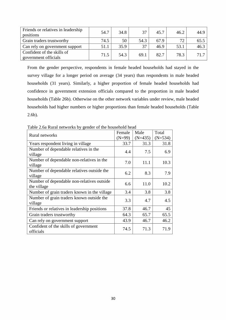
From the gender perspective, respondents in female headed households had stayed in the
survey village for a longer period on average (34 years) than respondents in male headed
households (31 years). Similarly, a higher proportion of female headed households had
confidence in government extension officials compared to the proportion in male headed
households (Table 26b). Otherwise on the other network variables under review, male headed
households had higher numbers or higher proportions than female headed households (Table
2.6b).
Table 2.6a Rural networks by gender of the household head
Rural networks Female
(N=99)
Male
(N=435)
Total
(N=534)
Years respondent living in village 33.7 31.3 31.8
Number of dependable relatives in the
village 4.4 7.5 6.9
Number of dependable non-relatives in the
village 7.0 11.1 10.3
Number of dependable relatives outside the
village 6.2 8.3 7.9
Number of dependable non-relatives outside
the village 6.6 11.0 10.2
Number of grain traders known in the village 3.4 3.8 3.8
Number of grain traders known outside the
village 3.3 4.7 4.5
Friends or relatives in leadership positions 37.8 46.7 45
Grain traders trustworthy 64.3 65.7 65.5
Can rely on government support 43.9 46.7 46.2
Confident of the skills of government
officials 74.5 71.3 71.9

31
CHAPTER THREE: ADOPTION OF SUSTAINABLE
AGRICULTURAL INTENSIFICATION PRACTICES (SAIPS)
3.1 Overview of SAIPs
Population growth in developing countries like Kenya is at all-time high and agricultural
resources are under pressure not only to provide food for the additional mouths but also to
provide livelihood for the majority of these populations that reside in rural areas with
agriculture as their main source of livelihood. In a country like Kenya where only a third of
its land mass is considered arable, this pressure to produce food and earn livelihoods will
likely push agriculture into fragile ecosystems of the country. The environmental
repercussions of extending agricultural activities in these fragile ecosystems are dire. The
alternative to circumventing this eminent problem is intensification of farming activities in
the high potential areas. There are a number of well researched and approved agricultural
intensification practices including but not limited to improved high yielding crop varieties
and animal breeds, approved agronomic practices including fertilizer, cereal/legume
intercropping, soil and water management practices, minimum/zero tillage and conservation
agriculture among many more practices. In this report we address the adoption of these
SAIPs though adoption of improved animal breeds is beyond the scope of this report.
3.2 Adoption spread of SAIPs
The results from descriptive analysis of adoption levels of SAIPs were as presented in Table
3.1a and Table 3.1b. The most widely adopted SAIPs across the five surveyed counties were
improved maize varieties, maize/legume intercropping, inorganic fertilizer and crop residue
retention on the farms (Table 3.1a). About 76% of the sampled households in the five
counties had adopted improved maize varieties. Eastern Kenya counties of Embu, Meru and
Tharaka had the highest adoption levels of improved maize varieties (88%, 91% and 92%,
respectively) while Siaya County in western Kenya had remarkably very low adoption rate
(39%). On the other hand, about 72% of the surveyed households had adopted maize/legume
intercropping technology. Contrary to the trends observed in adoption of improved maize
varieties, eastern Kenya Counties had the lowest adoption of maize/legume intercropping
technology compared to western Kenya counties. While the highest adoption of
maize/legume intercropping technology in eastern Kenya was 73% in Embu County,
Bungoma County in western Kenya had an adoption rate of 80% while Siaya County also in
western Kenya had an adoption rate of about 89% (Table 3.1a).

32
However, fertilizer adoption trends across the five sampled Counties was similar to adoption
trends of improved maize varieties i.e. eastern Kenya counties had higher proportions of
households that had adopted fertilizer compared to their western Kenya counterparts. The
overall adoption spread of fertilizer among the surveyed households was about 69% (Table
3.1a). Embu County had the highest proportion of households that had adopted fertilizer
(94%) while Siaya County again had the lowest proportion of households that had adopted
fertilizer (42%). On the other hand, crop residue retention adoption rate across the surveyed
counties was about 48%. Like maize/legume intercropping technology adoption rates,
western Kenya counties had the highest rates of crop residue retention on the farm compared
to their eastern Kenya counterparts. Siaya County had the highest proportion of households
that retained their crop residues on the farm (60%) while Tharaka County had the lowest
(39%).
Table 3.1a Adoption of SAIPs by county (% households)
SAIP
Bungoma
(N=137)
Tharaka
(N=81)
Embu
(N=93)
Meru
(N=81)
Siaya
(N=143)
Total
(N=535)
Improved maize variety 88 92 88 91 39 76
Maize legume intercropping 80 47 73 54 89 72
Inorganic fertilizer 61 85 94 86 42 69
Crop residue on the farm 49 39 42 41 60 48
Terraces 28 63 54 59 30 43
Grass strips 47 60 55 45 18 42
Maize legume rotation 19 57 28 34 8 26
Trees on boundaries 26 20 22 15 32 24
Minimum tillage 12 37 19 48 11 22
Conservation agriculture 2 8 2 3 4 4
Mechanized 25 3 7 28 8 14
Mulching 15 1 7 8 8 9
Soil bunds 1 3 4 10 2 3
The results of adoption of the most widely adopted SAIPs bring out several insights on the
farming systems across the two regions of eastern and western Kenya. First, it seems like
adoption of improved maize varieties go hand-in-hand with adoption of fertilizer. These two
intensification technologies were both more popular in eastern Kenya than western Kenya. It
is important to note that the two SAIPs are more capital intensive and need better market
access compared to the other two (maize/legume intercropping and crop residue retention)
that were more widely adopted in western Kenya than eastern Kenya. Therefore, eastern
Kenya farmers are generally better off in terms of poverty indicators compared to western
Kenya as demonstrated in national welfare monitoring surveys by the Kenya National Bureau

33
of Statistics. Equally important is the fact outlined in section 2 above that eastern Kenya
farmers practice more intensive agriculture compared to western Kenya farmers. For
example, the low levels of crop residue retention on the farms in eastern Kenya could be
associated with the fact that farmers in eastern Kenya are practicing intensive livestock
keeping practices like zero grazing and thus feed the crop residue to their livestock rather
than leaving it in the fields. These eastern Kenya farmers compensate crop residue retention
on the fields by applying fertilizer.
Further analysis was conducted to evaluate the adoption spread of SAIPs across households
headed by male and females. Again, considering the four widely adopted SAIPs in the five
surveyed counties, the results showed that a higher proportion of male headed households had
adopted improved maize varieties and fertilizer than those in the female headed households.
About 79% and 71% of male headed households had adopted improved maize varieties and
fertilizer, respectively, compared to 59% each among the female headed households (Table
3.1b). On the other hand, a higher proportion of female headed households had adopted
maize/legume intercropping and crop residue retention on the farms than those in male
headed households. About 82% and 53% of female headed households had adopted
maize/legume intercropping and crop residue retention, respectively, compared to 71% and
47% among the male headed households (Table 3.1b).
This gender analysis of adoption spread points out that more female headed households
adopted SAIPs that are less capital intensive while the converse was true for male headed
households. Therefore, the implication of these findings is that there is need to make female
headed households access capital that is needed for them to invest in improved seeds and
fertilizer. In the absence of capital, more intensive but less capital intensive technologies need
to be developed and availed to female headed households in order to improve their
productivity and welfare in general.
Table 3.1b Adoption of SAIPs by gender of the household head (% households)
SAIP Male (N=447) Female (N=88) Total (N=535)
Improved maize variety 79 59 76
Maize legume intercropping 71 82 72
Inorganic fertilizer 71 59 69
Crop residue on the farm 47 53 48
Terraces 44 39 43
Grass strips 44 32 42
Maize legume rotation 26 22 26

34
Trees on boundaries 24 24 24
Minimum tillage 22 19 22
Mechanized 15 10 14
Mulching 9 5 9
Conservation agriculture 3 5 4
Soil bunds 4 2 3
3.3 Adoption intensity of SAIPs
In order to mitigate against several crop production risks, farm households that adopt SAIPs
sometimes adopt them in combinations and not singularly. Descriptive analysis was carried
out to find out the number of SAIPs that households adopted and the results were as
presented in Figure 3.1, Table 3.2a and Table 3.2b. The SAIPs considered in this analysis
were improved maize varieties, fertilizer, maize legume intercropping, maize legume rotation
and minimum/zero tillage practices. From Figure 3.1, it is evident that the average number of
SAIPs adopted among the surveyed households across the five counties was about 3. Eastern
Kenya counties of Embu, Tharaka and Meru had higher adoption intensities compared to
their western Kenya counterparts. Tharaka and Meru Counties had the highest number of
SAIPs adopted per household i.e. about 3.2 each while Siaya county in western Kenya had
the lowest adoption intensity of about 2.3 (Figure 3.1).
2.93.2 3.0 3.2
2.3
2.8
0.00.51.01.52.02.53.03.5
Bungoma(N=137)
Tharaka (N=81) Embu (N=93) Meru (N=81) Siaya (N=143) Total (N=535)
Figure 3.1 Number of SAIPs adopted by County
The results from gender analysis of SAIPs adoption intensity were as presented in Figure 3.2.
Female headed households adopted less SAIPs (2.6) compared to male headed households
(2.9). Reasons for female headed households adopting less SAIPs are not clear but they could
be associated with female headed household having less capital, especially for the capital
intensive SAIPs like improved seed and fertilizer outlined in the preceding subsection 2.2.

35
Figure 3.2 Number of SAIPs adopted by gender of the household head
3.4 Impact of household resources on adoption intensity of SAIPs
Though there exists a wealthy empirical literature showing that SAIPs are very important in
increasing household agricultural productivity and thus income (Teklwold et al., 2014), the
adoption of these important technologies in developing countries like Kenya remains low. It
is therefore important to investigate the factors that condition household decision to adopt
SAIPs. In this report, kernel density graphs were used to shade light on how some selected
variables influenced household adoption decisions. Some of these variables included labour
availability and market access.
From Figure 3.2, it is evident that household with more labour, measured in terms of man
equivalent, were unlikely to adopt many SAIPs. The implication of this finding could be that
some of these SAIPs are labour reducing in terms of labour needed for some farm activities
like ploughing and weeding. For example a household that practices minimum till or
mulching is likely to spend less time on ploughing and weeding thereby saving on labour.
Therefore, households that are labour constrained are likely to adopt more SAIPs compared
to otherwise as shown in Figure 3.2.

36
11
.52
2.5
33
.5
Num
ber
of S
IPs a
dop
ted
0 5 10 15 20 25Total man equivalent
95% CI predicted numberSIPs
Figure 3.2 Relationship between number of SAIPs and household labour
Similarly, further analysis showed a generally negative relationship between distance to the
main market and SAIPs adoption intensity (Figure 3.3). This is particularly critical when it
comes to market sourced intensification technologies like improved seed and fertilizer. Given
the fact that there is empirical evidence to show that SAIPs can improve household welfare
significantly, there is need to shorten the distances between main markets and the households.
This distance shortening could be done in several ways including improving the transport and
communication infrastructure and or give traders who deal in these technologies incentives to
set up their distributional outlets in remote areas where these farmers are found. The
incentives could come in terms of tax exemptions or tax holidays for example.

37
1.5
22
.53
3.5
Num
ber
of S
IPs a
dop
ted
0 100 200 300Walking time to the main market (minutes)
95% CI predicted numberSIPs
Figure 3.3 Relationship between number of SAIPs adopted and distance to the main market
3.5 Conservation agriculture (CA)
Conservation agriculture was broadly defined to include three parameters i.e. minimum/zero
tillage, crop residue retention and maize legume intercropping. A household was considered
to have adopted conservations agriculture if he/she was found at least practicing the four
technologies at ago in at least one of his/her plots. About 4% of the surveyed households
were found to have practiced CA at least in one of their plots (Figure 3.4). Tharaka County
had the highest CA adoption rate of about 8% while Embu County had the lowest adoption
rate of about 2%. However, from a gender perspective, a higher proportion of female headed
households (5%) were found to have adopted CA compared the proportion among male
headed households (3%).

38
2
8
23
44
0
1
2
3
4
5
6
7
8
Bungoma(N=137)
Tharaka(N=81)
Embu(N=93)
Meru (N=81) Siaya(N=143)
Total(N=535)
Figure 3.4 Adoption of CA by County (% households)
3.5 Adoption of improved maize varieties
Maize is the main staple grain in Kenya and in fact, food security in the country is
synonymous with availability of maize. However, productivity of this main staple has not
kept pace with demand that is mainly driven by rapid increase in the population. Several
approaches have been proposed on how to increase maize productivity in the country. Top on
the proposal of increasing maize productivity has been wide dissemination and adoption of
improved maize varieties among smallholder farmers who constitute the largest proportion of
producers (about 75% of the maize produced in the country). Due to its importance in the
diets of almost all rural households in the country, and especially among the sampled
counties, almost all the surveyed households were found growing the crop (Figure 3.5).
In this section, results of descriptive statistics of maize adoption – both spread and intensity
are presented and discussed. Broad categories of improved maize varieties are considered i.e.
hybrid varieties, open pollinated varieties (OPVs) and combined hybrids and OPVs under the
category of improved maize varieties. Further descriptive analysis was also conducted to
assess the adoption of the four most widely adopted specific maize varieties among the
sampled households. These descriptive statistics are presented at the national level (full
sample), at the county level and at the gender of the household level in order to see the
variation across these major groupings.
3.5.1 Adoption spread of improved maize varieties
Adoption spread as adopted herein refers to the proportion of the surveyed households that
were found growing improved maize varieties. From the sampled households, about 97% of

39
these households had grown maize. This shows how important the crop is among the
cropping systems of the households in the sampled counties. On the other hand, about 75%
and 2% of the sampled households had adopted improved hybrid maize varieties and
improved OPV maize varieties, respectively (Figure 3.5). Overall the adoption spread of
improved maize varieties among the surveyed households was about 76%. Clearly, these
statistics show that hybrid maize varieties are more popular than OPVs among the sampled
households. Reasons for preference of hybrids over OPVs are not clear though they could be
related to productivity as it will be seen later in the successive parts of this section.
0
20
40
60
80
100
Grew maize Improvedhybrid
Improved OPV All improved(hybrid/OPV)
97
75
2
76
Figure 3.5 Adoption spread of improved maize varieties (% households) – N=535
Further descriptive analysis was carried out to assess the spread of different maize varieties
across the five sampled counties. The results showed that all sampled households in
Bungoma County and Embu County grew maize while Siaya County had the least proportion
of households that grew maize among the sampled counties (Table 3.2a). In terms of
improved maize varieties, the descriptive statistics results showed that Siaya County had
exceptionally the lowest proportion of households that grew improved hybrid maize varieties
i.e. while Siaya County had only 39% of the households growing hybrid maize varieties,
Tharaka County had 92%, Meru County had almost 89%, Bungoma County had 88% and
Embu County had 82% (Table 3.2a). Improved OPVs were only grown in Embu (10%) and
Meru Counties (4%). However, overall, the results showed higher proportion of sampled
farmers in eastern Kenya counties adopting improved maize varieties compared to western
Kenya. Tharaka County had the highest proportion of households that had adopted improved
maize varieties (92%), followed by Meru County (89%), Bungoma County (88%), Embu

40
County (87%) and then lastly Siaya County (39%). It is very apparent from these results that
concerted efforts need to be put in place to increase adoption of improved maize varieties in
Siaya district which lacks behind at less than 50% among the five sampled districts. Reasons
behind the extremely low levels of adoption of improved maize varieties in Siaya County
compared to the other sampled counties need to be investigated further and appropriate
measures taken to address this big technology adoption gap.
Table 3.2a Adoption spread of maize varieties by county (% households)
Maize variety
Bungoma
(N=137)
Tharaka
(N=81)
Embu
(N=93)
Meru
(N=81)
Siaya
(N=143)
Grew maize 100.0 97.5 100.0 96.3 93.0
Improved hybrid 88.3 92.4 82.3 88.8 39.2
Improved OPV 0.0 0.0 10.4 3.8 0.0
All improved
(hybrid/OPV) 88.3 92.4 87.5 91.3 39.2
From the gender perspective, the descriptive statistics showed that male headed households
had the highest proportion of households that had adopted the improved maize varieties
compared to female headed households. While almost 80% of the male headed households
had adopted improved maize varieties, less than 60% of the female headed households were
found to have adopted improved maize varieties (Figure 3.6). On the other hand, about 78%
of the male headed households had adopted improved hybrid maize varieties compared to
58% of the female headed households. About 3% of the male headed households had adopted
improved OPVs while only 1% of the female headed households had adopted this category of
improved maize varieties (Figure 3.6). Therefore, the adoption spread of improved maize
varieties by gender showed that low adoption spread among female headed households and
this could be caused by several factors. One of the reasons for low adoption rates f improved
maize varieties among female headed households could be that improved seeds of maize
varieties are capital intensive and female headed households could be disadvantaged in term
of capital compared to male headed households. Also, seeds of improved maize varieties
could be only found with stockists usually located in main markets that are in many cases at
far distances from markets. Since female farmers might be constrained more than male
farmers in accessing these markets in terms of transportation, (male farmers could ride
bicycled themselves to these markets), female farmers might not be able to access improved
seeds easily. Therefore, policies or interventions that could increase the input distributional
networks in rural areas could be important in enabling female headed households’ access
these important inputs.

41
78
3
79
58
1
59
0
20
40
60
80
100
Improved hybrid Improved OPV All improved (hybrid/OPV)
Male (N=447) Female (N=88)
Figure 3.6 Adoption spread of maize varieties by gender of the household head (%
households)
For specific improved maize varieties, the descriptive analysis showed that the top four most
widely adopted improved maize varieties in Kenya were DUMA43, H513, DK8031 and
WS505 in that order of reducing importance (Figure 3.7). About 29% of the total sampled
households grew DUMA43; followed by a distant 12% that grew H513, ten 11% who grew
DK8031 and lastly 8% growing WS505. All these for top most widely adopted improved
maize varieties are hybrids – a clear indication that OPVs are not very popular among the
surveyed households. Reasons for preference of hybrids over OPVs are not clear and need
further investigations. Similarly, more rigorous analysis of data is needed to tease out the
reasons why DUMA43 is more widespread among the surveyed households i.e. could it be a
market failure problem or special intrinsic variety specific traits.

42
0
5
10
15
20
25
30
DUMA43 H513 DK8031 WS505
29
1211
8
Figure 3.7 Adoption of the most widespread improved maize varieties (% households) –
N=535
Across the surveyed counties, the most popular improved maize variety, DUMA43, was more
widely adopted in Tharaka County (58%) followed by Embu County (57%), Meru County
(41%) and then Siaya County (13%). There was no adoption of DUMA43 in Bungoma
County (Table 3.3a). This means that DUMA43 is mainly grown in eastern Kenya Counties
compared to western Kenya counties. On the other hand, H513 was grown in all the five
sampled counties with the highest proportion of farmers in Meru County growing this variety
(35%) followed by Bungoma County (12%), Tharaka County (9%), Siaya County 8% and
then Embu County (3%). Siaya county had the histe proportion of households that grew
DK8031 (15%) followed by Tharaka and Meru County at about 14% each, Embu County at
12% and Bungoma County at less than 2%. WS505 was almost entirely grown in Bunoama
district only. Almost 28% of the households sampled from Bungoma district grew WS505
while just a paltry 1% of those from Embu County grew this variety and no households from
the other remaining three counties Table 3.3. The variation in adoption of specific varieties
across the counties could be associated with micro-climatic factors in those areas and or seed
and other market infrastructure related reasons i.e. seed companies in Kenya could be
targeting certain areas with their products more than other areas in the country for some
economic/business reasons.
Table 3.3 Adoption spread of most popular improved maize variety by county (%
households)
Maize variety
Bungoma
(N=137)
Embu
(N=93)
Tharaka
(N=81)
Meru
(N=81)
Siaya
(N=143)
DUMA43 0.0 57.0 58.8 40.7 13.3

43
H513 12.4 3.2 8.8 34.6 7.7
DK8031 1.5 11.8 13.8 13.6 15.4
WS505 27.7 1.1 0.0 0.0 2.1
3.5.2 Adoption intensity of improved maize varieties
Adoption intensity was analyzed in term s of how much land resources the household had put
under different maize varieties. From the results presented in Table 3.4a, almost 60% of the
land cultivated by the surveyed households was under maize. Siaya district had the highest
proportion of cultivated land that was under maize (72%) followed by Embu County (60%
and then Bungoma County (56%), Meru County (47%) and lastly Tharaka County (42%).
However, despite having the highest proportion of land under maize among the five surveyed
counties, Siaya district had the lowest proportion of maize area that was under improved
hybrid maize varieties across the five sampled counties (Table 3.4a). While the overall
adoption intensity of improved hybrid maize varieties among the surveyed households was
about 68% of the total maize area, Siaya district had only 31% of its maize area under I
improved hybrid maize varieties. The highest adoption intensity of improved hybrid maize
varieties was in Meru County (85%) and Bungoma County (84%). As expected, adoption
intensity of OPVs was very low i.e. only 1.7% of the total maize area among the surveyed
households was under OPV.
Table 3.4a Adoption intensity of maize varieties by county
Intensity variable
Bungoma
(N=137)
Embu
(N=93)
Tharaka
(N=81)
Meru
(N=81)
Siaya
(N=143)
Total
(N=535)
Percent cultivated area under
maize (%) 56.1 60.4 42.3 47.2 72.2 57.7
Percent maize area under hybrid
varieties (%) 84.3 76.6 81.6 84.7 31.3 68.4
Percent maize area under OPV
varieties (%) 0.0 6.9 3.0 0.0 0.0 1.7
Percent maize area under
improved varieties (%) 84.3 83.5 84.7 84.7 31.3 70.1
However, the broad analysis of improved maize varieties revealed that about 70% of the
maize area among the sampled households was under improved varieties (either hybrids and
or OPVs). Highest improved maize adoption intensities were in eastern Kenya counties with
Tharaka and Meru Counties having the highest adoption intensity of about 85% followed by
Bungoma County at 84%, Embu County at just slightly more than 83% and then lastly Siaya
County at just above 30% (Table 3.4a). Therefore the big question here is that why Siaya
district has the highest proportion of cultivated land under maize yet it has the lowest

44
proportion of cultivated land under improved varieties? If there are productively more
superior improved varieties suitable for Siaya agro-ecological zones, then why is the adoption
of these varieties very low in Siaya? Probably maize could be acting as a cash crop in Siaya
County thus the high allocation of its land to it. On the contrary, in the other four counties,
there are alternative cash crops. For example, in Bungoma district, the most widely adopted
cash crop is sugar cane grown under contract with Nzoia and Mumias sugar companies. On
the other hand, coffee and tea are very popular cash crops in the three eastern Kenya Counties
of Embu, Meru and Tharaka.
At the gender level, female headed households allocated more of their cultivated land to
maize than male headed households i.e. while female headed households allocated almost
70% of their cultivated land to maize, male headed households allocated only 55% of their
cultivated land to maize (Table 3.4b). One outstanding implication of this finding is that
female headed households give priority to food security and thus allocate more of their
cultivated land to the main food staple, maize, than male headed households. On the other
hand, male headed households are more risk takers and they allocate more land to cash crops
like sugar cane in Bungoma County of western Kenya and tea and coffee in Embu, Meru and
Tharaka Counties in eastern Kenya.
Table 3.4b Adoption intensity of improved maize varieties by gender of the household head
Intensity variable Male Female
Percent cultivated area under maize (%) 55.2 69.5
Percent maize area under hybrid varieties (%) 71.8 54.4
Percent maize area under OPV varieties (%) 1.8 1.0
Percent maize area under improved varieties (%) 73.6 55.4
However, in terms of adoption intensity of improved maize varieties, again male headed
households adopted improved maize varieties more intensively than female headed
households. About 74% of the maize area under male headed households was under
improved maize varieties compared to 55% of the maize area under female headed
households that was under improved maize varieties (Table 3.4b). Similarly, for improved
hybrid maize varieties, about 72% of the maize area under male headed households was
under improved hybrid maize varieties while about 54% of the maize area under female
headed households was under improved hybrid maize varieties. Lastly, male headed
households had also a higher adoption intensity of improved OPVs (2%) compared to female
headed households (1%).

45
This later finding on maize adoption intensity by gender also has far reaching implication on
overall national production of maize and by extension national food security. The implication
is that if high yielding maize varieties can be availed to female headed households, then
national maize production levels are likely to increase given the fact that female headed
households put a higher proportion of their cultivated land under maize production than their
male counterparts (Table 3.4b).
3.6 Maize productivity
As a main food crop in Kenya, maize productivity should keep pace with increase in demand
that is usually driven by population growth. Descriptive analysis of productivity of this crop
by variety type, county surveyed and gender of the household head was carried out and
results presented and discussed in this section.
The results showed that the overall maize productivity (yield) among the surveyed
households was about 1.4 t/ha. Among the improved maize varieties, hybrid maize varieties
were higher yielding than OPVs. The average yield for hybrid maize varieties was about 1.6
t/ha while that of OPVs was about 1.4 t/ha (Figure 3.8). Similarly, comparing the overall
improved maize productivity with local varieties showed that the former had a superior yield
than the latter. While the improved maize varieties yield was about 1.6 t/ha, local maize
varieties had a yield of about 0.9 t/ha (Figure 3.8). The implication of these results is that
there is need for concerted effort to popularize and promote the diffusion of improved maize
varieties among the sampled farmers in order to increase maize production and address the
food security problems affecting much of the rural farming households in the surveyed
counties.
0.0
0.5
1.0
1.5
2.0
Improvedhybrid
ImprovedOPVs
Allimproved
Local All varieties
1.61.4
1.6
0.9
1.4
Figure 3.8 Maize productivity by variety type (t/ha)

46
Across, the surveyed counties, the descriptive statistics showed that Meru County had the
highest maize productivity (yield) at about 1.8 t/ha followed by Bungoma County and
Tharaka County with 1.5 t/ha each, Embu County with 1.4 t/ha and Siaya County with the
least maize yield of just about 1 t/ha (Table 3.5a). Except the local maize varieties, Meru
County had the highest yield for all improved maize varieties than any other sampled county.
On the other hand, Siaya County had the lowest maize yield for all improved maize varieties
except the local varieties. The yield difference between improved and local varieties is
highest in Meru County and Bungoma County while it is lowest in Siaya County and Tharaka
County (Table 3.5a). The low yield difference between improved and local maize varieties
could be one of the contributing factors for low adoption spread and intensity of improved
maize varieties in Siaya County. Probably, improved maize varieties have a higher yield than
local variety when the production risks are low e.g. optimum rainfall, but the downside yield
risk in the event of the risk occurring is so high in improved maize varieties compared to
local maize varieties. This could be the reason that has forced maize farmers in Siaya to
continue growing local maize varieties as compared to farmers from the other sampled four
counties. In fact, Siaya County has the lowest annual average rainfall and is more prone to
drought compared to the other four counties (Tongrukswattana et al., 2015).
Table 3.5a Maize productivity by county (t/ha)a
Maize variety Bungoma Tharaka Embu Meru Siaya Total
Improved hybrid 1.6 1.6 1.5 1.9 1.2 1.6
Improved OPVs na na 1.3 1.7 na 1.4
All improved 1.6 1.6 1.5 1.9 1.2 1.6
Local 0.9 1.3 1.0 0.4 0.9 0.9
All varieties 1.5 1.5 1.4 1.8 1.0 1.4
a/: na means not applicable i.e. the variety was not grown in that particular county
At the gender level, the descriptive statistics showed that compared to female headed
households, male headed households had on average better maize yield on all varieties. The
overall maize productivity for male headed households was about 1.5 t/ha while that of
female headed households was just 0.9 t/ha. For the hybrid maize varieties, the yield of male
headed households was about 1.7 t/ha compared to 1.1 for female headed households.
Similarly, for the OPVs, the yield of male headed households was about 1.6 t/ha while that of
female headed households was less than 0.5 t/ha (Table 3.5b). On average, improved maize
productivity for male headed households was 1.6 t/ha while female headed households was
just 1 t/ha. The low maize productivity among female headed households as compared to

47
male headed households could be associated with the low levels of improved maize adoption
among female headed households as compared to male headed households (Figure 3.6).
Table 3.5b Maize productivity by gender of the household head (t/ha)
Maize variety Male Female Total t-statistic p-value
Improved hybrid 1.7 1.1 1.6 3.927 0.000
Improved OPVs 1.6 0.4 1.4 1.100 0.284
All improved 1.6 1.0 1.6 4.105 0.000
Local 1.0 0.8 0.9 2.359 0.019
All varieties 1.5 0.9 1.4 5.632 0.000
3.7 The economics of maize production
Farmers expend their resources in the process of producing maize. This maize produced is
used mainly for home consumption among smallholder farmers though sometimes they sell
surpluses at some given point in time. It is therefore proper for an in-depth analysis of costs
incurred in maize production process compared to the value of the grain harvested to
ascertain the economic attractiveness of maize production. The costs that go into the
production process are both fixed and variable (proportional) costs. In this section, we only
consider variable costs that will enable us to establish gross margins of maize production in
the framework of returns to land and family labour. Only cash purchased costs were
considered.
The descriptive statistics of maize gross margins across the five sampled counties were as
presented in Table 3.6a. The average gross margin of maize across the counties was about
KSh. 32,529 ha-1
. Bungoma County had the highest gross margins of about KSh. 47,000 ha-1
while Meru district had the lowest gross margins of about KSh. 21,587 ha-1
. Though Siaya
County had the lowest maize productivity and thus the lowest value of maize produced per
hectare of area under maize, this county had the third highest maize gross margins, beating
Embu and Meru counties. The implication of this result could be that though Meru and Embu
had higher yields of maize, the yields in these two districts come with a heavy capital outlay
in terms of yield enhancing inputs like improved seeds and fertilizers. In fact, the total
variable costs of the three eastern Kenya counties (Embu, Meru and Tharaka) were almost 4
times that of Siaya County (Table 3.6a). A striking observation wothy highlighting is that
herbicide and pesticide use on maize crop is more popular in eastern kenya counties
compared to western kenya copunties. On the other hand, hiriong of oxen in maize
production was more popular in western kenya than eastern Kenya (Table 3.6). The latter
finding is in line with the earlier finding where a higher proportion of households from
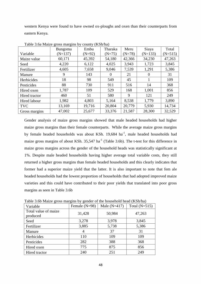
48
western Kenya were found to have owned ox-ploughs and oxen than their counterparts from
eastern Kenya.
Table 3.6a Maize gross margins by county (KSh/ha)
Variable
Bungoma
(N=137)
Embu
(N=92)
Tharaka
(N=75)
Meru
(N=78)
Siaya
(N=133)
Total
(N=515)
Maize value 60,171 45,392 54,180 42,366 34,230 47,263
Seed 4,220 6,122 4,025 3,943 1,723 3,845
Fertilizer 4,605 7,658 9,046 7,539 1,291 5,386
Manure 9 143 0 21 0 31
Herbicides 18 98 549 45 1 109
Pesticides 88 730 911 516 14 368
Hired oxen 1,787 109 529 168 1,001 856
Hired tractor 460 51 580 9 121 249
Hired labour 1,982 4,803 5,164 8,538 1,779 3,890
TVC 13,169 19,716 20,804 20,779 5,930 14,734
Gross margins 47,002 25,677 33,376 21,587 28,300 32,529
Gender analysis of maize gross margins showed that male headed households had higher
maize gross margins than their female counterparts. While the average maize gross margins
by female headed households was about KSh. 19,684 ha-1
, male headed households had
maize gross margins of about KSh. 35,547 ha-1
(Table 3.6b). The t-test for this difference in
maize gross margins across the gender of the household heads was statistically significant at
1%. Despite male headed households having higher average total variable costs, they still
returned a higher gross margins than female headed households and this clearly indicates that
former had a superior maize yield that the latter. It is also important to note that fem ale
headed households had the lowest proportion of households that had adopted improved maize
varieties and this could have contributed to their poor yields that translated into poor gross
margins as seen in Table 3.6b
Table 3.6b Maize gross margins by gender of the household head (KSh/ha)
Variable Female (N=98) Male (N=417) Total (N=515)
Total value of maize
produced 31,428 50,984 47,263
Seed 3,278 3,978 3,845
Fertilizer 3,885 5,738 5,386
Manure 4 37 31
Herbicides 110 109 109
Pesticides 282 388 368
Hired oxen 775 875 856
Hired tractor 240 251 249

49
Hired labour 3,168 4,060 3,890
TVC 11,743 15,437 14,734
Gross margins 19,684 35,547 32,529
Further analysis of the significance of particular cost items was conducted and results were as
presented in Figure 3.9. Fertilizer constituted the highest proportion of total maize variable
costs among the surveyed households. About 37% of the total maize variable costs were
fertilizer followed by seed and hired labour at about 26% each (Figure 3.9). These results
points to the fact that for maize to become more profitable, then fertilizer costs has to be
minimized significantly. Therefore, the use of less capital intensive productivity enhancing
technologies like maize/legume intercropping and rotation, crop residue retention and other
approved CA techniques becomes hand in making maize more profitable to smallholder
farmers in Kenya.
37
26
26
7
3
Fertilizer Seed Hired labour
Hired oxen/tractor Others (pesticides etc)
Figure 3.9 Variable costs contribution (%)
3.8 Adoption of inorganic fertilizer
Due to deteriorating soil fertility as a result of continuous cultivation of plots, fertilizer
application has been used for a long time as a way to restore soil fertility and thus increase or
maintain crop productivity. Despite this obvious benefit, adoption spread and adoption
intensity of fertilizer in sub-Saharan African countries like Kenya is still low compared to
other developing and developed countries in the world. Like in the previous section on maize
adoption, fertilizer adoption spread was analyzed by getting the proportion of the surveyed
households that had used fertilizer. On the other hands, fertilizer adoption intensity was the
amount of fertilizer that was used per given area. Analysis of adoption intensity of fertilizer
was extended to unconditional and conditional adoption intensities. Unconditional intensity is
where all cultivated area was considered as the denominator while conditional adoption
intensity is where only plots that had applied fertilizer were used as denominators.

50
3.8.1 Fertilizer adoption spread
Almost 87% of the surveyed households in the five counties had adopted fertilizer. The
highest adoption spread was mainly in eastern Kenya counties compared to the western
Kenya counties. Embu County had the highest proportion of sampled households that had
adopted fertilizer (96%) followed by Meru county (93%) and Bungoma County (91%). Siaya
County had the lowest proportion of households that had adopted fertilizer in their crop
production activities at 79% (Table 3.7a). A higher proportion of the surveyed households
had adopted basal fertilizer (85%) compared to top dressing (62%). Basal fertilizer adoption
was higher in the eastern Kenya counties (Embu, Meru and Tharaka) compared to western
Kenya counties (Bungoma and Siaya). Overall, Siaya district had the lowest adoption of both
basal and top dressing fertilizers among the five surveyed counties (Table 3.7a).
Table 3.7a Adoption spread of fertilizer by county (% households)
Fertilizer type
Bungoma
(N=137)
Tharaka
(N=79)
Embu
(N=96)
Meru
(N=80)
Siaya
(N=143)
Total
(N=535)
Planting (basal) 83.9 84.8 92.7 87.5 77.6 84.5
Top dressing 73.7 69.6 71.9 83.8 29.4 62.4
All 90.5 89.9 95.8 92.5 79.0 88.6
From a gender perspective, a higher proportion of male headed households adopted fertilizer
compared to the proportion in female headed households. Whereas 90% of the male headed
households had adopted fertilizer, only 81% of the female headed households had adopted
fertilizer (Table 3.7b). The proportion of female headed households who had adopted basal
and top dressing fertilizer was lower than that of male heeded households and particularly for
the top dressing fertilizers. The low adoption of fertilizer among female headed could be
associated with high capital outlay that is required for a household to adopt fertilizer. It could
also be associated with the bulkiness of fertilizer thus disadvantaging female heeded
household to transport it to their farms.
Table 3.7a Adoption spread of fertilizer by gender of the household head (% households)
Fertilizer Male (N=447) Female (N=88) Total (N=535)
Planting (basal) 85.2 80.7 84.5
Top dressing 66.7 40.9 62.4
All 90.2 80.7 88.6
3.8.2 Fertilizer adoption intensity
Considering all cultivated area, the unconditional fertilizer adoption intensity was computed
by sampled county and by gender of the household head. The overall unconditional adoption

51
rate of fertilizer among the surveyed households was about 90 kg/ha. Embu County had the
highest adoption rate of about 126 kg/ha followed by Bungoma County at about 107 kg/ha
(Table 3.8a). On the other hand, Siaya County had the lowest unconditional fertilizer
adoption rate of just about 34 kg/ha. These results show that the county with the highest
adoption rate applies more than three times what the lowest county applies. For specific
fertilizer types, the descriptive statistics showed that the average adoption rate of planting
(basal) fertilizer was about 60 kg/ha while that of top dressing was about a half of the basal
i.e. 30 kg/ha (Table 3.8a). Siaya district had the lowest adoption rates for both basal and top
dressing among the five surveyed counties. The unconditional adoption rate for top dressing
fertilizer was particularly low for top dressing fertilizer in Siaya County compared to
Bungoma County that had the highest rate of applying top dressing fertilizer (Table 3.8a).
Table 3.8a Unconditional fertilizer adoption intensity by county (kg/ha)
Fertilizer
Bungoma
(N=574)
Tharaka
(N=561)
Embu
(N=586)
Meru
(N=519)
Siaya
(N=641)
Total
(N=2881)
Planting (basal) 59.5 59.6 88.9 69.4 26.0 59.8
Top dressing 47.1 26.8 37.0 34.6 8.3 30.2
All 106.5 86.4 125.9 104.0 34.3 90.0
Further descriptive analysis of the unconditional fertilizer application rates at the gender of
the household head was conducted and the results were as presented in Table 3.8b. Overall,
female headed households applied unconditionally low rates of fertilizer compared to male
headed households. While male headed households had on average unconditional fertilizer
application rate of about 93 kg/ha, female headed households had about 72 kg/ha. Similarly,
male headed households had a higher rate of applying both planting (basal) and top dressing
fertilizer than female headed household though the difference in top dressing was lower
compared to that of the basal fertilizers. Both male and female headed households almost
applied twice as much planting (basal) fertilizer as they did with top dressing fertilizer (Table
3.8b).
3.8b Unconditional fertilizer adoption intensity by gender of the household head (kg/ha)
Fertilizer Male (N=2467) Female (N=414) Total (N=2881)
Planting (basal) 62.1 45.7 59.8
Top dressing 30.8 26.4 30.2
All 93.0 72.1 90.0
Adoption intensity of fertilizer was also analyzed conditional on having applied fertilizer on
that particular plot i.e. by considering only plots that had fertilizer applied on them. The

52
overall results in this analysis showed that the rate of applying fertilizer was about 212 kg/ha
up from 90 kg/ha when all cultivated plots were considered (Table 3.8c and Table 3.8a,
respectively). At county level, conditional adoption intensity results showed that Bungoma
had the highest rate of about 283 kg/ha compared to just about 107 kg/ha when all cultivated
plots were considered in Table 3.8a. Therefore, while Embu County had the highest
unconditional adoption rate among the sampled counties, Bungoma County had the highest
conditional adoption rates. At this point, it is important to note that Bungoma County could
be having high conditional adoption rates due to fertilizer credit facility availed by Nzoia
Sugar Company for application of the same on sugar cane by the contracted farmers. On the
contrary, the other four sampled counties might be having such kind of arrangements.
Table 3.8c Conditional fertilizer adoption intensity by county (kg/ha)
Fertilizer Bungoma Tharaka Embu Meru Siaya Total
Planting (basal) 183.7 162.1 157.1 154.2 120.4 154.6
Top dressing 175.1 92.0 94.8 93.3 112.7 115.6
All 283.0 209.5 204.8 209.9 153.7 212.3
Similar analysis of conditional adoption rates of fertilizer was conducted for male and female
headed households and results presented in Table 3.8d. The results still showed that male
headed households had a higher fertilizer adoption rates than female headed households. For
instance, male headed households had overall conditional fertilizer application rate of about
217 kg/ha up from 93 kg/ha compared to about 180 kg/ha up from 72 kg/ha for female
headed households (Table 3.8b and Table 3.8d, respectively).
3.8d Conditional fertilizer adoption intensity by gender of the household head (kg/ha)
Fertilizer Male Female Total
Planting (basal) 159.6 123.1 154.6
Top dressing 114.4 125.6 115.6
All 217.4 179.5 212.3
3.9 Fertilizer application on maize crop
Maize productivity is very important in determining national food security in Kenya. A part
from providing food, maize is also an important source of cash income for smallholder
farmers who manage to produce surplus for the market. Therefore enhancing its productivity
is very critical for national poverty eradication and enhanced food security. To achieve higher
productivity of maize, use of improved seed and fertilizer has been promoted by both public
and private efforts. Use of improved maize was discussed in details in section 3.5. In this

53
section, we present and discuss the results of use of fertilizer on maize crop among the
surveyed households.
About 69% of the surveyed households applied some fertilizer on their maize crop. Fertilizer
application on maize crop was more prevalent among the households in eastern Kenya
counties of Embu, Tharaka and Meru compares to farmers from western Kenya counties of
Bungoma and Siaya (Table 3.9a). Embu County had the highest proportion of households
that applied fertilizer on their maize crop at almost 94% followed by Meru County at 86%,
Tharaka County at almost 85% and Bungoma County at about 61%. Siaya County had the
least proportion of the households that applied fertilizer on their maize crop at just about
422% (Table 3.9a). About 65% of the households in the five surveyed counties had used
some planting (basal) fertilizer on their crop compared to about 50% who had used top
dressing fertilizer on their maize crop. Across all the surveyed counties, there were more
households that used planting (basal) fertilizer on their maize crop than those who used top
dressing fertilizer (Table 3.9a).
Table 3.9a Adoption spread of fertilizer on maize crop by county (% households)
Fertilizer
Bungoma
(N=137)
Tharaka
(N=79)
Embu
(N=96)
Meru
(N=80)
Siaya
(N=143)
Total
(N=535)
Planting (basal) 51.8 78.5 91.7 82.5 40.6 64.5
Top dressing 48.9 65.8 65.6 73.8 17.5 49.7
All 60.6 84.8 93.8 86.3 42.0 69.0
Similarly, a higher proportion of male headed households had adopted fertilizer on their
maize crop than the proportion among the female headed households. Overall, whereas
almost 71% of the male headed households had adopted fertilizer on their maize crop, only
59% of female headed households had adopted fertilizer on their maize crop (Table 3.9b). A
higher proportion of both male and female headed households adopted planting (basal)
fertilizer on their maize crop compared to top dressing fertilizer. In fact, the proportion of
female headed households that applied planting (basal) fertilizer on their maize crop is almost
double that one that applied top dressing (Table 3.9b).
Table 3.9b Adoption spread of fertilizer on maize crop by gender of the household head (%
households)
Fertilizer
Male
(N=447)
Female
(N=88)
Total
(N=535)
Planting (basal) 66.0 56.8 64.5
Top dressing 52.8 34.1 49.7

54
All 70.9 59.1 69.0
Fertilizer application intensity (rates) on maize crop was analyzed and results presented in
Table 3.10a – 3.10d. Unconditional application rates of fertilizer to maize crop showed an
overall application rate of about 114 kg/ha among the surveyed households. It was clear from
these results that unconditional fertilizer application rates on maize were higher in eastern
Kenya counties than western Kenya counties. This higher adoption intensity in eastern Kenya
could be associated with the fact that more households use fertilizer on their crop in eastern
than western Kenya as shown in Table 3.9a. The amount of planting fertilizer used on maize
crop was more than twice the top dressing fertilizer. An average of about 9 kg/ha of top
dressing fertilizer was unconditionally applied to maize crop compared to about 21 kg/ha for
the planting (basal) fertilizer. However, the difference in unconditional top dressing and basal
fertilizer application rates on maize in Bungoma County was not that big like in the other four
sampled counties (Table 3.10a).
Table 3.10a Unconditional adoption intensity of fertilizer on maize crop by county (kg/ha)
Fertilizer
Bungoma
(N=574)
Tharaka
(N=561)
Embu
(N=586)
Meru
(N=519)
Siaya
(N=641)
Total
(N=2881)
Planting (basal) 64.3 93.5 121.6 98.5 21.3 73.1
Top dressing 51.9 48.9 53.5 64.9 8.7 40.9
All 116.3 142.4 175.2 163.4 30.1 114.0
At the gender, level, male headed households had a higher unconditional fertilizer application
rate compared to female headed households among the surveyed households. Whereas female
headed households had an average of about 84 kg/ha, male headed households had almost
121 kg/ha (Table 3.10b). Similarly, female headed households had consistently lower
unconditional application rates of planting (basal) and top dressing fertilizers compared to
their male headed counterparts.
Table 3.10b Unconditional adoption intensity of fertilizer on maize crop by gender of
household (kg/ha)
Fertilizer Male (N=2467)
Female
(N=414)
Total
(N=2881)
Planting (basal) 77.2 53.9 73.1
Top dressing 43.3 29.7 40.9
All 120.5 83.7 114.0
For the conditional analysis, the descriptive statistics showed that the average overall
fertilizer application rate on maize crop was about 187 kg/ha up from 114 kg/ha (Table 3.10c

55
and Table 3.9c, respectively). Bungoma district had the highest conditional fertilizer
application rates on maize crop (239 kg/ha) while Siaya County had the lowest (102 kg/ha).
This means that among the five surveyed counties, maize production is more seriously
undertaken in Bungoma County where farmers undertake heavy capital outlays in terms of
buying fertilizer just to improve the productivity of this crop. The general higher fertilizer
application rates observed in eastern Kenya counties (table 3.8c) could be associated with the
fact that they apply most of that fertilizer in cash crops like coffee and tea or in other high
value crops other than maize. The conditional planting (basal) and top dressing fertilizer
application rates showed higher rates for the former than the later i.e. about 97 kg/ha of top
dressing fertilizer was applied to maize crop on average compared to about 129 kg/ha for the
planting (basal) fertilizer (Table 3.10c).
Table 3.10c Conditional adoption intensity of fertilizer on maize crop by county (kg/ha)
Fertilizer Bungoma Tharaka Embu Meru Siaya Total
Planting
(basal) 157.7 133.5 145.1 120.7 74.3 129.0
Top dressing 145.5 87.0 88.5 89.6 83.6 97.5
All 239.1 189.6 199.1 186.6 101.9 187.0
On the other hand, male headed households had a higher conditional fertilizer application rate
on maize compared to female headed households. About 190 kg/ha of fertilizer was applied
to maize crop by male headed households while about 168 kg/ha was applied to maize by
female headed households (Table 3.10d). Male headed households had consistently higher
conditional application rates of both planting (basal) and top dressing fertilizers compared to
female headed households.
Table 3.10d Conditional adoption intensity of fertilizer on maize crop by gender of household
(kg/ha)
Fertilizer Male Female Total
Planting (basal) 131.9 112.2 129.0
Top dressing 97.0 101.7 97.5
All 190.2 168.0 187.0
3.10 Determinants of technology adoption: Multivariate probit regression estimates
The descriptive results of the multivariate Probit model variables are presented in Table 3.11
and the econometric results in Table 3.12. The econometric results indicate that social
economic and plot characteristics such as age, education, fertility, slope, depth and soil colour
significantly influence technology adoption. The probability of adopting herbicide use and

56
minimum tillage technologies reduces with education. More educated farmers showed a
higher probability of adopting knowledge intensive technologies and ones that require
considerable input in terms of management such as improved seed and soil and water
conservation similar to findings by Pender & Gebremedhin (2007). Again, educated farmers
may also be more aware of the benefits accrued to adoption of modern technologies and more
able to search for appropriate technologies to alleviate constraints in production (Pender &
Gebremedhin, 2007, Kassie et al. 2011).
The probability of adopting animal manure and legume intercrop increased with age. Older
farmers have accumulated much experience in farming to understand the substitution of
fertilizer with manure. They also adopt legume intercrop as a risk diversifying strategy
especially in some parts of eastern region. Farmers who perceived their plots as good or
moderately good in terms of fertility did not adopt fertilizer use, soil and water conservation
and minimum tillage. These two technologies are mainly adopted with an intent to improve
the fertility of the soil and hence less likely that they are adopted in relatively fertile soils.
Plots in Eastern region which is the reference were more likely to adopt improved seed,
minimum tillage, fertilizer and pesticide use but less likely to adopt legume intercrop. Sub
plot distance significantly influenced adoption of fertilizer, improved seed, soil and water
conservation and animal manure. Distance which is a proxy for accessibility can influence the
use of inputs, availability of information as well as opportunity cost of labour (Jansen et al.
2006; Wollni et al. 2000; Pender & Gebremedhin 2007). Distance increases the amount of
labour by raising the output input price ratios (Shiferaw et al. 2012).
Table 3.11: Description and measurement of variables
Dependent variables Description and measurement of variables Mean Std. Dev.
Fertuse Plot received fertilizer (1=yes; 0= no) 0.76 0.42
Pestuse Plot received pesticide (1=yes; 0= no) 0.27 0.44
Herbuse Plot received herbicide (1=yes; 0= no) 0.04 0.20
Impseed Plot received improved seed (1=yes; 0= no) 0.75 0.43
Mintill Plot received minimum tillage (1=yes; 0= no) 0.09 0.29
Swatercons Plot received soil water conservation (1=yes; 0= no) 0.54 0.49
Animan Plot received animal manure (1=yes; 0= no) 0.39 0.48
leg_interc_p Plot received legume intercropping (1=yes; 0= no) 0.20 0.40
Legcrrop Plot received legume crop rotation (1=yes; 0= no) 0.16 0.36
Independent variables Mean Std. Dev.
Mzyieldpacre Maize yield per acre in kilograms 147.75 925.33
Age The age of the farmer (years) 51.28 14.46
Educ Education level of the farmer in years of schooling 7.93 7.47

57
Season Farming season during the year (1=long rains 0=short
rains)
0.47 0.499
Subplotdist Distance to the subplot from home in kilometers 6.96 25.14
Subplotarea Area of the subplot in acres 0.33 1.09
Howmanycrops Number of crops grown on the subplot 1.83 0.73
Goodffertpt Farmer perceives soil fertility to be good (1=yes; 0=
no)
0.16 0.37
Modffertpt Farmer perceives soil fertility to be moderate (1=yes;
0= no)
0.48 0.49
porffertpt
(reference)
Farmer perceives soil fertility to be poor (1=yes; 0=
no)
0.08 0.27
flatsloplt (reference) Farmer perceives soil slope to be flat (1=yes; 0= no) 0.33 0.47
Modsloplt Farmer perceives soil slope to be moderate (1=yes; 0=
no)
0.34 0.47
Steepsloplt Farmer perceives soil slope to be steep (1=yes; 0=no) 0.053 0.22
shallow_depthplot
(reference)
Farmer perceives soil depth to be shallow (1=yes;
0=no)
0.09 0.28
mod_depthplot Farmer perceives soil depth to be moderate (1=yes;
0=no)
0.23 0.42
deep_depthplot Farmer perceives soil depth to be deep (1=yes; 0=no) 0.39 0.48
blacksoil (reference) Farmer perceives soil type to be black (1=yes; 0=no) 0.10 0.31
Brownsoil Farmer perceives soil type to be brown (1=yes; 0=no) 0.40 0.49
Redsoil Farmer perceives soil type to be red (1=yes; 0=no) 0.16 0.37
Greysoil Farmer perceives soil type to be grey (1=yes; 0=no) 0.04 0.19
Residue Crop residues & stubble were left on sub-plot from
previous season (2011/12) (1=yes; 0=no)
0.42 0.55
age_sq Age squared 2839.61 1573.74
stress_inc_e The farmer experienced stress incidence (1=yes; 0=
no)
0.69 0.46
western (reference) Region of residence (1=yes 0=no ) 0.49 0.50
Eastern
Region of residence (1=yes 0=no )
0.50
0.50
Decfemales Female is the decision maker in cropping activities
(1=yes; 0=no)
0.15 0.35
decmales Male is the decision maker in cropping activities
(1=yes; 0=no)
0.12 0.32
joint_decsn Joint decision making in cropping activities (1=yes;
0=no)
0.50 0.50
extmaz Farmer had access to extension services (1=yes; 0=
no)
0.46 0.49
Lnincome Log of farmers income 10.98 1.31

58
Table 3.12: Multivariate probit model parameter estimates across SAI packages
Variable Fertilizer (FT) Pesticide (PT) Herbicide (HB)
Coef Std. Err Coef Std. Err Coef Std. Err
Mzyieldpacre 0.0002* 0.0001 0.0001*** 0.00002 -0.00003 0.0001
Age -0.008 0.009 0.002 0.006 -0.008 0.013
Educ 0.011 0.028 0.005 0.017 -0.083 0.045
Season -0.185 0.170 -0.295** 0.138 -0.338 0.240
Subplotdist 0.018* 0.010 0.0001 0.005 -0.0002 0.009
Subplotarea 0.025 0.062 -0.023 0.030 0.024 0.052
Howmanycrops 0.130 0.145 0.220** 0.101 -0.156 0.191
Goodffertpt -0.161 0.358 -0.023 0.291 0.460 0.472)
Modffertpt -0.068 0.304 -0.067 0.238 -0.474 0.403
Modsloplt 0.397* 0.217 0.009 0.163 0.257 0.317
Steepsloplt -0.416 0.427 -0.436 0.323 0.420 0.463
mod_depthp_t -0.177 0.322 -0.315 0.234 0.182 0.421
deep_depth_t -0.152 0.284 -0.587*** 0.216 -0.111 0.398
Brownsoil 0.195 0.285 0.725*** 0.267 -0.135 0.451
Redsoil 0.265 0.333 1.462*** 0.293 0.471 0.491
Greysoil 1.083** 0.547 0.214 0.407 0.131 0.600
Residue 0.195 0.162 0.213** 0.086 -0.506* 0.281
age_sq 0.000 0.0001 -0.0001 0.0001 -0.0002* 0.0001
stress_inc_e -0.124 0.199 -0.259 0.159 -0.036 0.298
Eastern 0.623*** 0.200 1.146*** 0.167 0.725** 0.302
fem_decsn 5.021 131.5 -0.478** 0.213 -0.493 0.504
joint_decsn -0.298 0.191 0.067 0.167 0.532 0.356
Extmaz -0.111 0.197 -0.193 0.161 0.418 0.280
Inincome 0.104 0.070 0.084 0.057 0.051 0.120
Variables Improved seed
(IS)
Minimum Tillage
(MT)
Soil Water Conservation
(SWC)
Coef Std Err Coef Std Err Coef Std Err
mzyieldpacr 0.0001 0.0001 0.000 0.000 0.0000 0.000
Age -0.0001 0.007 -0.016* 0.010 0.0070 0.004
Educ -0.016* 0.013 -0.051** 0.025 0.023* 0.015
Season -0.239* 0.124 -0.080 0.153 0.036 0.112
subplotdist 0.014* 0.007 0.001 0.007 -0.013** 0.005
subplotarea 0.042 0.064 -0.055 0.113 0.053 0.045
howmanycr
o
-0.052 0.107 0.084 0.121 0.186** 0.091
goodffertpt -0.063 0.264 - 0.3145 0.448* 0.236

59
0.831***
modffertpt -0.201 0.213 -
0.889***
0.246 0.096 0.195
modsloplt 0.300*
*
0.151 0.750*** 0.195 0.181 0.136
steepsloplt 0.010 0.334 0.193 0.431 0.2913 0.292
mod_depthp
_t
-0.0407 0.229 -0.018 0.273 -0.2960 0.205
deep_depth- -0.226 0.205 -0.064 0.243 -0.077 0.183
brownsoil 0.198 0.188 0.160 0.283 -0.057 0.176
Redsoil 0.345 0.230 0.914** 0.306 -0.178 0.209
Greysoil -0.348 0.284 -0.215 0.472 -1.111*** 0.309
Residue -0.125 0.091 0.232** 0.103 -0.174* 0.093
age_sq 0.000 0.0001 -0.0001 0.0001 0.0000 0.0001
stress_inc_e 0.125 0.145 -0.036 0.186 -0.127 0.133
Eastern 0.380*
**
0.142 0.503** 0.177 0.067 0.129
fem_decsn -0.260 0.175 -0.059 0.253 -0.278* 0.162
joint_decsn 0.033 0.161 0.560** 0.211 0.061 0.143
Extmaz -0.092 0.138 0.066 0.178 0.246* 0.128
lnincome 0.027 0.051 0.1023 0.069 0.041 0.047
Variables Animal Manure (AM) legume intercrop
rotation(LI)
legume crop
rotation(LCR)
Coef Std Err Coef Std Err Coef Std Err
Mzyieldpacre 0.000 0.00002 0.0000 0.00002 0.000 0.0001
Age 0.011* 0.006 0.017** 0.007 -0.017** 0.007
Educ 0.012 0.008 0.0008 0.017 0.006 0.018
Season -0.125 0.113 -0.106 0.128 -0.104 0.151
subplotdist -0.022*** 0.006 0.006 0.006 -0.012 0.008
subplotareaH -0.025 0.027 -0.020 0.029 0.021 0.034
howmanycro
p
0.053 0.092 0.369*** 0.101 -0.197 0.117*
goodffertpt 0.007 0.235 0.357 0.260 0.319 0.310
modffertpt -0.275 0.196 0.245 0.216 0.250 0.267
modsloplt 0.171 0.137 0.094 0.153 -0.111 0.184
steepsloplt 0.124 0.306 -0.307 0.325 0.713** 0.316
mod_depthp_ -0.078 0.206 0.064 0.226 -0.487 0.256
deep_depth_t -0.067 0.182 -0.125 0.201 -0.464** 0.235
brownsoil 0.234 0.184 -0.459** 0.219 0.311 0.268
Redsoil 0.287 0.214 -1.020*** 0.248 0.795*** 0.286
Greysoil -0.272 0.298) -0.092 0.358 -0.452 0.519

60
Residue 0.010 0.0871 -0.023 0.093 -0.015 0.126
age-sq 0.0001** 0.00005 -0.0001* 0.00006 0.0000 0.00007
stress_inc_e 0.278** 0.136 -0.067 0.152 -0.065 0.173
Eastern -0.202 0.131 -0.354** 0.144 0.038 0.172
fem_decsn -0.163 0.1655 0.102 0.197 -0.439* 0.224
joint_decsn 0.341** 0.146 -0.442*** 0.164 -0.038 0.180
Extmaz -0.284** 0.129 0.162 0.147 -0.013 0.168
lnincome 0.026 0.047 -0.037 0.054 -0.067 0.062
Notes: Coef means coefficient
***, ** and * denote statistical significance at 1%, 5% and 10% confidence levels,
respectively.

61
3.11 SAI Packages use across maize, beans and maize-bean intercrop sub-plots
The SAI package combinations are presented on Table 3.13 and the multinomial regression
results on package used combinations
Table 3.13: SAI packages used on pure maize and bean stands and maize bean intercrop plots
Choice j Binary quadruplet
(package)
Improved
Seed (S)
S1 S0
Organic
Fertilizer (F)
F1 F0
Animal
Manure(M)
M1 M0
Pesticide (P)
P1 P0
1 S1 F0 M0 P0 √ √ √ √
2 S0 F1 M0 P0 √ √ √ √
3 S0 F0 M1 P0 √ √ √ √
4 S0 F0 M0 P1 √ √ √ √
5 S1 F1 M0 P0 √ √ √ √
6 S1 F0 M1 P0 √ √ √ √
7 S1 F0 M0 P1 √ √ √ √
8 S0 F1 M1 P0 √ √ √ √
9 S0 F1 M0 P1 √ √ √ √
10 S0 F0 M1 P1 √ √ √ √
11 S1 F1 M1 P0 √ √ √ √
12 S1 F1 M0 P1 √ √ √ √
13 S1 F0 M1 P1 √ √ √ √
14 S0 F1 M1 P1 √ √ √ √
15 S1 F1 M1 P1 √ √ √ √
NOTE: The binary quadruplets represent the possible SAI combinations. Each element in the
quadruplet is a binary variable for adoption of improved seed (S), organic fertilizer (F), animal
manure (M) and pesticide (P) and 0 = otherwise.
3.12 Factors explaining the adoption decision of SAI packages
The results from multinomial logit model presented in Table 3.14 are compared to the reference
package of fertilizer and improved seed (S1F1M0P0). The education level of farm decision maker
positively influence uptake of (S0F1M1P1) and (S1F1M1P1) packages but has a negative effect on

62
adoption of (S1F1M0P1) and (S1F0M1P1) packages. This might be because a package combining
use of fertilizer, improved seed and pesticide is relatively knowledge intensive and requires
considerably higher management skills. Highly educated farmers are able to search for
information and interpret extension services. SAIs are knowledge intensive and requires
considerably higher management skills
The age of household head positively influence adoption of packages (S1F1M1P0), (S1F1M0P1),
(S0F1M1P0,), (S0F1M0P0,) and (S1F0M0P0), but negatively related to the adoption of (S1F0M1P1)
package. Age being a proxy for experience in farming, the elderly tend to adopt more of fertilizer
and manure packages.
There is a strong positive correlation between sex of plot decision maker and adoption of
(S1F0M1P0) package. Similarly adoption of (S1F1M0P1) and (S1F0M0P0) packages are also
positively influenced by sex of plot decision maker. Male farmers tend to adopt more of
improved seed and fertilizer.
The results further indicate the importance of soil fertility in determining adoption of (S0F1M0P0)
and (S0F1M0P1) packages. This could be because when the soil fertility is good farmers do not
use fertilizer. Farmers who perceive their plots to be fertile have low adoption of packages
containing fertilizer. With good soil fertility there is little use of fertilizer.
The adoption of (S1F1M1P1), (S0F1M1P1), (S1F0M1P1) and (S1F1M1P0) packages is negatively
influenced by the area of farmer’s sub plot. Farmers who have small pieces of land use more than
two technologies on their sub plots, probably because they intend to increase production so as to
have adequate food for their families. Farmers who have small pieces of land use more than two
technologies on their sub plots.
Farmers’ income positively influences uptake of (S1F1M1P1), (S0F1M1P1), (S1F0M0P1) and (S1F0
M0 P1), but negatively influence uptake of (S0F1M1P0) packages. Farmers’ income influences
uptake of more SAI technologies more so those that had fertilizer.. This can also be attributed to
the fact that most farmers pointed out the prices of fertilizer and improved seed to be a major
challenge.

63
Availability of labor was found to be crucial in adoption of (S0F0M1P0), (S0F1M1P0), (S0F1M0P1)
and (S1F1M1P1) Packages. This could be because packages containing fertilizer, manure and
pesticide tend to use more labor. Probably because they are labor intensive.

64
Table 1: Factors explaining the adoption decision of SAI packages
Variable F S M SM SP FM FP MP SFM SFP SMP FPM SFMP
Education
level
0.002
(0.013)
-0.024
(0.053)
-0.062
(0.071)
-0.050
(0.065)
-0.038
(0.140)
0.007
(0.017)
0.029
(0.035)
0.158
(0.225)
0.003
(0.013)
-0.043*
(0.024)
-0.720***
(0.347)
0.033*
(0.019)
0.023**
(0.011)
Age 0.014**
(0.007)
-0.010
(0.014)
0.038**
(0.017)
0.033
(0.016)
0.010
(0.036)
0.017*
(0.010)
0.045
(0.029)
0.024
(0.063)
0.020***
(0.06)
0.018***
(0.007)
-0.02***
(0.043)
0.008
(0.018)
0.018
(0.007)
Sex of plot
decision
maker
-0.2418**
(0.104)
0.826***
(0.298)
1.599
(0.528)
1.146***
(0.394)
0.714
(0.754)
-0.246
(0.157)
1.051
(0.742)
0.475
(0.788)
0.134
(0.092)
0.253**
(0.109)
2.990
(1.452)
0.290
(0.312)
0.048**
(0.108)
Subplotdista
nce
-0.013*
(0.008)
-0.001
(0.011)
-0.099
(0.066)
-0.096
(0.055)
-0.050
(0.072)
0.004
(0.006)
0.027*
(0.015)
-0.011
(0.059)
-0.001
(0.004)
0.001
(0.004)
-0.090
(0.394)
-0.041
(0.047)
-0.005
(0.006)
Soil fertility 0.414***
(0.154)
-0.365
(0.322)
-0.017
(0.410)
-0.757
(0.394)
-0.262
(0.856)
0.307
(0.238)
0.562
(0.749)
0.361
(1.257)
-0.255
(0.131)
0.093
(0.150)
3.264
(1.988)
-0.185
(0.433)
-0.217
(0.156)
Group
membersh
0.036
(0.185)
-0.188
(0.364)
-0.826
(0.510)
0.145
(0.476)
-14.912
(899.17
-0.060
(0.278)
0.767
(0.899)
0.616
(0.037)
-0.058
(0.155)
-0.186
(0.181)
-1.290*
(0.800)
-0.448
(0.510)
-0.337
(0.184)
Subplot
tenure
-0.020
(0.176)
-1.085
(0.737)
0.021
(0.568)
0.699**
(0.292)
0.796***
(0.473)
-0.938**
(0.478)
-1.885
(0.260)
-1.402
(0.958)
-0.442**
(0.185)
0.229
(0.148)
-14.610*
(0.300)
-1.523
(0.876)
-0.666
(0.259)
Subplotarea -0.013
(0.116)
0.100
(0.116)
-0.097
(0.318)
-0.043
(0.233)
-0.393
(0.965)
0.071
(0.116)
-1.354
(1.075)
0.082
(0.296)
-0.030**
(0.077)
0.048
(0.085)
-2.943**
(2.658)
-1.511*
(0.806)
-0.050***
(0.113)
Income 0.430***
(0.106)
-0.173
(0.159)
-0.106
(0.233
-0.100
(0.221)
0.258
(0.479)
0.078***
(0.160)
-0.008**
(0.659)
0.202
(0.769)
-0.075
(0.093)
0.003
(0.007)
-0.063
(0.774)
0.774*
(0.334)
0.117**
(0.210)
Labour -0.005
(0.007)
-0.016
(0.012)
-0.050**
(0.023)
-0.020
(0.016)
-0.011
(0.033)
-0.001*
(0.009)
0.020**
(0.009)
-0.014
(0.052)
0.004
(0.005)
-0.133
(0.113)
0.037
(0.032)
0.023
(0.010)
0.021*
(0.005)
_cons -1.943***
(0.553)
-1.272
(1.396)
-5.936***
(1.937)
-4.743***
(1.579)
-5.298
(3.240)
-2.108**
(0.912)
0.238
(0.29o)
-1.020
(0.662)
-0.689
(0.478)
-2.080***
(0.598)
0.463
(0.300)
1.879
(0.877)
-0.534
(0.559)
Number of
observation
s
3,449
Note: Standard errors are in parenthesis. Fertilizer and Improved seed (FS) is the reference package. S= improved seed, F= organic fertilizer,
M= animal manure, P= pesticide
***, ** and * denote statistical significance at 1%, 5% and 10% confidence level.

65
Group membership influenced the adoption of (S1F0M1P1) package .This is attributed to the fact
that farmers in groups get more information easily and share them among themselves. With
limited or inadequate information sources and imperfect markets, including insurance market and
social networks could facilitate the exchange of information hence aid farmers to get inputs on
time and overcome other challenges including credit constraints.
3.13 Impact of farmers' choice of SAI technology combination on labour use and income
With regard to SAI uptake on labor use, results reveal that farmers who adopted SAI packages
significantly demand more labor than it would have been if they had not adopted the specified
SAI packages as shown on Table 3.15. Similarly adoption of packages containing three or four
technologies per plot demanded more labor than packages that had one or two technologies. The
results further showed that packages containing manure and pesticide use demanded the highest
amount of labor. This is probably because manure use and pesticide application is labor
intensive.
On the other hand, adoption of packages contained minimum tillage and soil and water
conservation significantly decreased labor demands. This result contradicts the findings by
Hailemariam et al. (2013) who analyzed the impacts of cropping system diversification,
conservation tillage and modern seed adoption on household income, agrochemical use and
demand for labor in Ethiopia, and found that conservation tillage increased pesticide application
and labor demand. This is probably due to the fact that initial costs of putting up ridges and
farrows for minimum tillage could be very high and very low cost if any in the consecutive years.
Hence the costs of maintaining minimum tillage and soil and water conservation are very
minimal in the consecutive years resulting to decreased labor demands.
Concerning the impact of farmers' choice of SAI technology combination on income, results
generally reveal that adoption of SAI practices in combination increases farmer’s income than
adoption in isolation. The highest proceeds are achieved when SAI practices are adopted in
combination rather than in isolation.
The results also show that adoption of packages that contain soil and water conservation and
minimum tillage gives the highest income. Previous studies have shown that conservation tillage
can lead to substantial ecosystem service benefits by reducing soil erosion and nutrient depletion
and conserving soil moisture (Fuglie, 1999; Woodfine, 2009).

66
Table 2: Impact of SAI practices combinations on labor use in man days and income.
ATT SAI Mean of labor use Mean of income
SF 26.402(0.605) 46794(1780)***
SM 27.758(0.857) 34852(1345)
SP 28.630(0.981) 37968(1704)
FM 27.378(0.814) 34310(1260)***
FP 26.878(0.628) 45344(1964)***
MP 28.527(0.584) 36091(781)
SFM 30.168(1.373) 36948(3406)
SFP 28.693(0.991) 37444(1638)
SMP 30.219(1.360) 37069(3365)
SMFP 30.168(1.373) 39588(3366)**
WT 24.702(2.186) 45919(3871)
ST 26.170(1.785) 52437(7885)*
WTS 24.787(1.458)* 45071(3817)
WTH 25.950(0.611)* 47879(1249)**
WTM 25.028(0.995)* 37868(2055)
WCT 25.317(0.755) 32893(1436)***
WTFM 26.629(0.819) 43945(4180)***
WTCS 25.317(0.755)** 32893(1436)***
WTPF 26.395(0.258) 43945(4180)***
WTCSF 24.357(0.768)** 48003(1469)***
ATU SF 21.749(0.881)*** 33794(1780)***
SM 27.758(0.857) 34852(1345)
SP 23.856(0.574)** 37968(1704)
FM 24.336(0.666) 34310(1260)***
FP 21.681(0.897)*** 49344(1964)***
MP 20.444(1.036)** 36091(781)
SFM 24.651(0.556) 36948(3406)
SFP 23.897(0.574)** 37444(1638)
SMP 24.627(0.557) 37069(3365)
SMFP 24.651(0.556) 39588(3366)**
WT 21.682(1.790)*** 45919(3871)
ST 20.931(0.770)*** 52437(7885)*
WTS 22.505(0.513)* 45071(3817)
WTH 25.369(0.709) 44219(1249)**
WTM 24.518(0.660) 37868(2055)
WCT 26.212(0.671) 32893(1436)***
WTFM 22.107(1.893)* 43945(4180)***
WTCS 26.212(0.671) 32893(1436)***

67
Note: Standard errors are in parenthesis. S= improved seed, F= organic fertilizer, M= animal manure, P=
pesticide, C=Intercrop, T=Minimum tillage, W =Soil and water conservation.
***,
** and
* denote significance at 1%, 5% and 10% confidence level.
The highest income of 52437 Kenya shillings is achieved when improved seed variety is used
under minimum tillage followed by use of improved seed, minimum tillage, fertilizer, soil and
water conservation and intercropping package that gave 48003 Kenya shillings. However, it also
appears that use of fertilizer and improved seed variety enables farmers to earn higher income
from their farm produce.
The uptake of package containing minimum tillage, soil and water conservation and herbicide
also gives a higher output of farm produce. Perhaps, because conservation agriculture may
necessitate application of herbicides to kill weeds before planting under minimum tillage
systems. This is in-tandem with other studies which have revealed that system diversification
helps to maintain soil biodiversity, which can reduce pest and weed infestations that otherwise
must be controlled by pesticides and/or additional labor (Hajjar et al., 2008; Tilman et al., 2002).
Most packages that farmers use that contain use of improved seed varieties also contain the use
of pesticide. Besides, past studies have related the use of more pesticides in the package that
contains improved seed to the fact that farmers would like to avoid risk, as high yielding
varieties are prone to pest outbreaks (Jhamtani, 2011: Hailemariam et al., 2013).
As shown on Table 3.16, the average labor demand both for females and males is significantly
higher than it would have been if the adopters had not adopted. Adoption of SAI packages
increases women workload contributed to both family and hired labor compared to their male
counterparts. This puts different effects on male and female labor time allocation. In nearly all
cases, adoption of SAI packages leads to more time spent working on the farm for females than
for males. This may negatively affect larger households by diverting time from other activities
such as food preparation and childcare, as women are usually responsible for routine care of the
household. This is consistent to the findings by Njeri, (2007) who noted that in Kenya, women
WTPF 25.797(1.621) 43945(4180)***
WTCSF 20.994(0.667) 43003(1469)***

68
supply about 70-75 percent of agricultural labor in agriculture. Unlike men, women lack access
and control over production resources such as land, information and credit.
In general, adoption of SAI packages increases women workload contributed to both family and
hired labor compared to their male counterparts. More women depend on agriculture wage labor
as a source of livelihood. This is in line with the findings of Njeri (2007) who found that in
African societies, women are responsible for feeding their families hence crops produced for
subsistence are associated with women, while men grow cash crops because they are responsible
for providing cash income for the family.

69
Table 3.163: Impact of SAI practices combinations on labor use in man days by gender Family labor Women Family labor Men Hired labor Women Hired labor Men
ATT SF 9.970(0.252) 6.799(0.226) 2.413(0.071)*** 1.390(0.042)***
SM 10.655(0.289) 6.914(0.264)** 2.849(0.103)** 1.636(0.076)
SP 11.309(0.348)** 7.039*** 2.854(0.125) 1.722(0.091)
FM 10.626(0.265)*** 6.779(0.241)*** 2.759(0.092)** 1.551(0.078)
FP 9.229(0.250)*** 7.571(0.264)*** 2.360(0.078)*** 1.492(0.039)***
MP 9.742(0.224)*** 7.486(0.282)*** 3.226(0.113)*** 1.651(0.050)
SFM 11.239(0.589)** 6.871(0.488) 3.283(0.228)* 1.802(0.156)
SFP 10.007(0.395)*** 6.311(0.341)*** 2.861(0.125) 1.719(0.091)
SMP 10.082(0.557)** 6.970(0.477) 3.243(0.227)* 1.809(0.155)
SMFP 9.270(0.551)*** 8.347(0.590) 3.283(0.228)* 1.802(0.156)
ATU SF 9.521(0.420)*** 5.302(0.341)** 2.236(0.130) 1.180(0.075)***
SM 9.490(0.233)*** 5.670(0.209) 2.531(0.083)*** 1.769(0.070)***
SP 9.221(0.204)* 5.829(0.178) 2.568(0.085) 1.585(0.055)***
FM 9.578(0.231) 5.699(0.201) 2.529(0.082)*** 1.732(0.075)**
FP 9.469(0.437)*** 5.346(0.351)** 2.261(0.133) 1.177(0.071)***
MP 9.311(0.479)* 4.985(0.465) 2.455(0.185)*** 1.036(0.074)***
SFM 9.592(0.271) 6.164(0.194) 2.552(0.123)* 1.582(0.076)
SFP 9.507(0.252)** 5.885(0.218) 2.548(0.084) 1.575(0.054)***
SMP 9.713(0.227) 6.158(0.195) 2.562(0.128)* 1.589(0.075)
SMFP 9.145(0.236)* 6.452(0.241)** 2.552(0.123)* 1.582(0.076)
Note: Standard errors are in parenthesis.
1 man day = 8 working hours; S= improved seed, F= organic fertilizer, M= animal manure, P= pesticide.
***,
** and
* denote significance at 1%, 5% and 10% confidence level.
Source: Adoption Pathways Survey data, 2013

70
3.14 Relationship between farm size, family size and SAI intensity
The relationship between farm and family sizes, and SAI practices’ uptake intensity is given
in Figure 23. The results show that Bungoma County report the highest family size on
average, followed by Siaya County with a mean of 7 and 6 persons per household,
respectively. Embu County has the least household size with a mean 4 persons per household.
In Tharaka Nithi and Meru Counties households have an average of 5 persons.
Farmers from Siaya County have the largest parcels of land followed by Meru County with
an average of 5.14 and 5.06 acres per household. Embu County has small pieces of land with
an average of 2.95 acres per household.
On the contrast, Bungoma County reported the lowest number of plot SAI practices intensity
with a mean adoption rate of 3.99 per plot. Generally farmers use a package of four SAI
technologies per plot across the five Counties.
Figure 3.10: Relationship between farm size, family size and SAI intensity
3.15 Correlation of maize yield per acre with SIMLESA technologies
In Figure 24, the correlations between maize yields and the intensity of SAI practices are
presented. The results show that maize yield hectare and the use of improved seed variety
were highly correlated compared to all other SIMLESA technologies. This is expected since
the use improved maize varieties and fertilizer are relatively inseperable considering that two
constitute a package in the pursuit of the green revolution benefits.

71
Figure 3.2: Correlation of maize yield per acre with SIMLESA technologies
The correlation coefficient of 0.34 is significantly different from zero implying that adoption
of improved seed technologies is linearly linked with increased maize yield per unit area.
Minimum tillage and herbicide use technologies had minimum but positive correlation with
maize yield. However the coefficients are not significantly different from zero indicating that
though the correlation is positive, the degree of covariability is relatively negligible.

72
CHAPTER FOUR: AGRICULTURAL INPUT USE
4.1 Proportion of female labour in different crop production activities
The effects of SAI practices and labour use intensity is one of the issues that is not yet clear
cut in comparison to the conventional agricultural land use practices, especially when the
gender dimension and labour use is considered. In Table 4.1, a mean comparison of labour
use by gender is presented. The t test statistic shows significant differences between means
for labor man days provided by males and females in all farming activities. Females provided
bulk of family labor in the plots than males.
Table 4.1: Means of labor contribution by gender
Variable Female N=4298 Male N=4298 t
Total labor man days 5.41 (9.10) 3.95 (8.29) 7.75*
Land preparation and planting 1.27 (1.18) 1.07 (1.00) 3.08*
Weeding 1.70 (3.86) 0.98 (2.71) 10.11*
Harvesting 1.50 (3.64) 1.30 (4.67) 2.17**
Threshing 0.95 0.61 7.64*
Notes: Figures in parenthesis are standard deviations.
** and * denote significant at 5% and 10% confidence levels, respectively.

73
4.2 Maize seed sources and recycling between hybrids and OPVs and overall in maize as
a crop
Figure 4.1 show the sources of maize seed that farmers use in their fields. The results show
that a majority of the farmers in all the sampled counties sourced their first maize seed from
agro dealers and agro-vets. No maize seeds were sourced from extension demo plots and on
farm trials in Siaya and Bungoma counties. Likewise, farmers never soured seeds from
research centres in Meru and Bungoma counties.
Figure 4.1: Sources of maize seeds
Seeds supply to farmers by the government is observed in all counties being more prominent
in Siaya County at 6.25%. Farmer to farmer seed exchange is popular in Embu County with
11.43% of the farmers getting their seeds from this source. Local seed producers supplied
seeds to farmers in Embu and Bungoma counties compared to none in the other three
counties sampled.
4.3 Sources of information on new seed varieties by Gender and County
Majority of information among farmers on new seed varieties is obtained from fellow
neighboring farmers and other farmer relatives. Although agro dealers supplied majority of
seeds to farmers in all the counties, they conveyed very limited information on seed varieties.
However, they conveyed a proportion of this information in at least all the counties sampled.
Electronic and print media is the second most reliable source of this information in all the
counties sampled while farmer groups form of collective action failed to convey any
information in Siaya and Tharaka Nithi counties. Close to 17%, 10% and 11% of farmers in

74
Tharaka Nithi, Bungoma and Meru counties obtained this information from government
extension while failing to provide any information in Siaya and Embu counties.
4.4 Overview of main legumes grown across the survey counties (% households
growing)
Among the five major legumes grown in Kenya, beans were the most popular legume grown
in the five counties (Figure 4.2 and Figure 4.3)). Tharaka Nithi, Embu and Meru Counties
recorded high percentage of farmers growing beans in their households. Beans adoption rate
was relatively lower counties in western Kenya that is Bungoma and Siaya. Very few farmers
adopted soy, pigeon peas, groundnuts and cowpeas across the five counties.
0
20
40
60
80
100
120
Bungoma Tharaka Embu Meru Siaya Total
% h
ou
seh
old
s G
row
ing
Beans soy pigeon peas goundnuts cow peas
Figure 3: Main legumes grown across the counties

75
0
10
20
30
40
50
60
70
80
bean soy pigeon gnuts cow peas
% o
f fa
rme
rs
female male
Figure 4.3: Main legumes grown by gender of household head
Further analysis of legume grown across the counties based on gender reveal that more male
headed households adopted the legumes compared to female headed households.
4.5 Adoption of different varieties of the main legume grown in the country
Bean was the major legume grown across all the counties (Figure 4.4). In terms of adoption
of the bean varieties Mwitemania bean variety was the most popular followed by Rosecoco
and Wairimu the other three varieties Nyayo, Gacera Gacugu were not popular in all the
Counties. Mama safi bean variety was adopted by quite a number of farmers Embu only.
Mwitemania was not popular in western Kenya with Bungoma County recording few
households growing while in Siaya no farmer had adopted the variety. Majority of the
farmers in Siaya grew the Rosecoco beans variety.
0
10
20
30
40
50
60
70
80
90
% h
ou
seh
old
s gr
ow
ing
Bungoma Tharaka Embu Meru Siaya

76
Figure 4.4: Main bean varieties grown across the counties
Analysis of beans varieties grown by gender reveal that Wairimu, Mwitemania, Gacera and
Katheri were adopted more by male headed households while Rosecoco ,Nyayo,Gacugu and
Mama Safi was popular in female headed households (Figure 4.5).
0.005.00
10.0015.0020.0025.0030.0035.0040.0045.0050.00
% o
f fa
rme
rs g
row
ing
Female Male
Figure 4: Main bean varieties grown by gender of household head%
4.6 Main source of information of beans varieties
Source of information on major on agricultural technology is an important aspect in it
enhancing technology diffusion and uptake. The majority of the farmers in the five counties
received information on bean varieties from neighbors and relatives (Figure 4.6).
Surprisingly, major key institutions such as government extension, farmer groups, research
organizations were mot been used by farmers to get accurate information on the available
varieties

77
Figure 4.6: Main source of information of beans varieties
4.7 Main source of information of beans varieties by gender of household head
(%households)
A further look at the households sources of information on bean varieties from a gendered
perspective indicate that majority of the female headed household preferred accessing
information from a neighboring farmer who is not a relative (Figure 4.7)
0
10
20
30
40
50
60
70
% h
ou
seh
old
s
Female Male
Figure 5: Main source of information of beans varieties
Similarly as in maize production, high fertilizer prices and availability are a major constraint
highly ranked among the farmers sampled as a key issue in legume production (Figure 4.8).
Constraints in output and input market were observed in 6% and 8% of the sampled farmers

78
and were ranked between 6 and 7 in terms of concern to farmers with regard to other
constraints. Availability of credit to buy fertilizers and improved legume seeds were also
observed in 10% of the farmers. Timely availability of improved seed is a constraint to only
4% of the farmers sampled compared to 6% in maize production.
Figure 4.8: Constraints in accessing key inputs in legume production

79
CHAPTER FIVE: HOUSEHOLD WELFARE OUTCOME
5.1 Household food security
The subjective own assessment of household food security status was carried out during the
survey at household level. The descriptive statistics showed that about59% of the surveyed
household felt that they were food secure i.e. they had either food surplus or were at break-
even (no shortage and no surplus). Specifically, about 14% of the surveyed households
reported that they had food surplus while almost 45% were at the break-even point in terms
of food security (Figure 5.1). On other hand, about 37% of the sampled households reported
that they were having transitory food insecurity with almost 4% facing acute/chronic food
insecurity.
3.7
37.4 44.5
14.4
58.9
020406080
Chronic foodinsecurity
Transitoryfood insecurity
Break-evenfood security
Food surplusthrought
Overall foodsecure
Figure 5.1 Household food security (% households
Across the five sampled counties, the descriptive statics of food security showed that eastern
Kenya counties had the highest proportion of the households that were food secure compared
to western Kenya counties (Table 5.1). The county with the highest proportion of the
households that were food secure was Tharaka (almost 79%) while Bungoma County had the
lowest proportion of the households that felt that they were food secure (41%). It is important
to remember that these were own subjective assessments of food security by the main
household respondents in the survey and should be interfered from that perspective.
Table 5.1 Household food security by county (% households)
Maize variety
Bungoma
(N=137)
Tharaka
(N=79)
Embu
(N=96)
Meru
(N=80)
Siaya
(N=143)
Chronic food insecurity 5.8 1.3 4.2 2.5 3.5
Transitory food insecurity 53.3 20.3 30.2 27.5 42.0
Break-even food security 34.3 54.4 45.8 50.0 44.8
Food surplus throughout 6.6 24.1 19.8 20.0 9.8
Overall food secure 40.9 78.5 65.6 70.0 54.5

80
From a gender analysis perspective, the descriptive statistics of household food security
showed that male headed households were generally more food secure than female headed
households. About 60% of the male headed households were food secure compared to about
51% of the female headed households (Figure 5.2). Specifically, while a higher proportion of
male headed households were food surplus and break-even, a higher proportion of female
headed households were facing chronic and transitory food insecurities (Figure 5.2).
3.1
36.5
44.5
15.9
60.4
6.8
42.0 44.3
6.8
51.1
0
10
20
30
40
50
60
70
Chronic foodinsecurity
Transitory foodinsecurity
Break-even foodsecurity
Food surplusthrought
Overall foodsecure
Male (N=447) Female (N=88)
Figure 5.2 Household food security by gender of the household head (% households)

81
CHAPTER SIX: HOUSEHOLD INCOMES, RISKS AND LIVELIHOOD
SHOCKS
6.1 Household incomes
Rural farm households derive incomes to support their livelihoods from various sources. Due to
the risky environment in which they operate, they keep a portfolio of incomes ranging from
farming (crop and or livestock) to other non-farm activities like wage earning engagements and
business. Descriptive analysis was conducted first to ascertain the level of household incomes by
Survey County and by gender of the household head. The overall average household annual
income excluding income derived from livestock sales was about KSh. 156,000. The eastern
Kenya counties of Embu, Meru and Tharaka had the highest level of average household income
compared to western Kenya counties of Bungoma and Siaya (Figure 6.1). Embu County had the
highest level of average annual household income at about KSh. 229,000 while Siaya district had
the lowest average annual household income of about KSh. 106,000. Therefore the county with
the highest average annual household income (Embu) had an average household average income
that was more than twice that one of the lowest county (Siaya).
0
50
100
150
200
250
Bungoma(N=137)
Tharaka(N=81)
Embu(N=93)
Meru (N=81) Siaya(N=143)
Total(N=535)
146.9 150.1
229.2
193.1
106.4
156.1
Figure 6.1 Total household income excluding livestock (1,000 KSh)
Male headed households on the other had had a higher level of average household annual income
compared to female headed households. Whereas female headed households had an average
annual household income of about KSh. 94,000, male headed household had an average of about
KSh. 170,000 (Figure 6.2). This means that male headed households had an income that was
about twice that of female headed households. The implication of such huge income disparities

82
between male headed and female headed households is that the former are greatly disadvantaged
in access key resources to improve their livelihoods. These livelihood improving resources
include agricultural productivity inputs like purchased improved seed and fertilizer as seed in the
preceding sections of this report.
0
50
100
150
200
Female (N=88) Male (N=447) Total (N=535)
94.5
170.2156.2
Figure 6.2 Household incomes by gender of the household head (1,000 KSh)
Further analysis to gain more insight on the importance of different income portfolios in
household income was carried out. The results showed that overall, crop income accounted for
the largest share in in total household annual income among the surveyed households followed
by self-employment. About 40% of the total annual household income was from crops and 22%
was from self-employment (Figure 6.3). These results clearly indicate that crop enterprises
among the surveyed smallholder farmers are of great importance in their livelihoods. Therefore,
interventions aimed at improving on-farm productivity of crops are likely to go a long way in
reducing poverty and food insecurity among the rural farming communities in Kenya.

83
Figure 6.3 Household income shares (% share in total annual income)
Crop income still accounted for the highest proportion of total annual household incomes in all
the five surveyed counties. It was particularly important in Embu County where almost 70% of
the total household annual income was derived from crops (Table 6.1). On the other hand, Siaya
County had the lowest proportion of crop income in total annual household income at just 22%.
Generally, a comparison across the five districts reveals that crop income is more important in
the household incomes of the eastern Kenya households compared to western Kenya (Table 6.1).
Western Kenya households had the highest contribution on income from self-employment and
transfers compared to eastern Kenya households. It is also worth noting that higher proportions
of household incomes coming from transfers among the western Kenya households could be a
pointer to the fact that there is high dependence ration of western Kenya households on incomes
from those household members who have out-migrated in search of better opportunities
elsewhere. The low contribution of crop income in household income among Siaya households
could also be an indicator that the agro-ecological zones in this county are not favorable for crop
farming/production compared to the other sampled counties.
Table 6.1 Household income sources by county (% share in total income)
Source
Bungoma
(N=137)
Tharaka
(N=81)
Embu
(N=93)
Meru
(N=81)
Siaya
(N=143)
Total
(N=535)
Crops 29 49 69 48 22 40
Non-agricultural wages 25 19 9 19 16 18
Agricultural wages 6 13 5 5 5 7

84
Self-employment 25 12 11 20 33 22
Transfers & others 13 6 4 4 22 12
Gender analysis of the income shares of different sources revealed that male headed households
derived a higher proportion of their income from crops compared to female headed households
i.e. about 42% of the male headed households’’ income was from crops compared to 32% for
women headed households (Figure 6.4). Several reasons could be at play in explaining why male
headed households had a higher proportion of their income coming from crops than female
headed households. These reasons could include but not limited to accessibility to crop
production assets like land and other productivity enhancing inputs like improved seed and
fertilizer. Female headed household could be disadvantaged in accessing these assets. Male
headed households also had a higher proportion of income derived from agricultural wages, self-
employment and transfers compared to that of female headed households (Figure 6.4). It is also
worth noting that female headed households had a higher proportion of income coming from
non-agricultural wages than male headed households.
32
10 10
24 23
42
20
6
21
9
0
5
10
15
20
25
30
35
40
45
Crops Non-agriculturalwages
Agriculturalwages
Self employment Transfers &others
Female (N=88) Male (N=447)
Figure 6.4 Household income shares by gender of the household head (% shares in total income)
6.2 Household risks and livelihood shocks
The frequency of shocks as reported by the sample farmers across gender are reported in Figures
6.5 – 6.13. With regard to drought in the past ten years most female headed household were
affected two times more male headed households and this difference was statistically

85
significant. High incidences of hailstorms were recorded in Bungoma and Siaya counties. The
incidence in most cases occurred once in the past ten years.
High incidences of pests and diseases were recorded in Bungoma and Siaya counties. Pests and
diseases in most cases affected households once in the past ten years. High incidences of too
much rains and floods were recorded in Tharaka Nithi and Siaya counties. Too much rains and
floods in most cases affected households once in the past ten years. High incidences of drought
were recorded in Tharaka Nithi, Embu and Meru counties. Drought in most cases affected
households once in the past ten years but for those households in siaya the frequency of
occurrence for drought was more than to times.
Frequency of increase in food prices (past five years) by gender of the household head is
presented in Figure 6.11. High incidences of increase in food prices were recorded in Bungoma
County. Increase in food prices in most cases affected households once in the past ten years in
Embu and Meru while Tharaka Nithi and Siaya recorded more than two times.
Frequency of increase in input prices (past five years) by gender of the household head is
presented in Figure 6.12. Increase in input prices in most cases affected households once in the
past five years in with exemption of siaya recorded more than two times. Frequency of decrease
in output prices (past five years) by gender of the household head is presented in Figure 6.13.
Risk of decrease in output prices was higher in Tharaka Nithi, Embu and Meru and low in Siaya
and Bungoma counties.
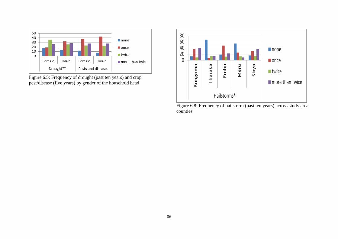
86
Figure 6.5: Frequency of drought (past ten years) and crop
pest/disease (five years) by gender of the household head
Figure 6.8: Frequency of hailstorm (past ten years) across study area
counties

87
Figure 6.7: Frequency of pest and diseases (past ten years) across
study area counties
Figure 6.9: Frequency of too much rains and floods (past ten years)
across study area counties
Figure 6.10: Frequency of drought (past ten years) across study area
counties
Figure 6.12: Frequency of increase in food prices (past five years)
across study area counties

88
Figure 6.11: Frequency of increase in input prices (past five years)
across study area counties
Figure 6.13: Frequency of decrease in output prices (past five years)
across study area counties

89
Percent reduction of main crop production and overall incomes due to risks across counties
are given in Figure 6.14 (refer figure below) . The results suggest that percent reduction of
either main crop production or overall household income by drought is generally higher.
Percent reduction on crop yields due to drought is highest in Embu and Bungoma and on
income is highest in Tharaka Nithi and Embu. Hailstorms highly reduced crop yields in
Tharaka Nithi.
Percent reduction of main crop production and overall incomes due to risks across according
to the gender of the household head is presented in Figure 6.15 (refer figure below). The
results indicate that percent reduction of either main crop production or overall household
income as a result of risks is higher in female headed households. Percent reduction on crop
yields and income due to drought is higher.

90
Figure 6: percent reduction of main crop production and overall incomes due to risks across counties
Figure 6.15: Percent reduction of main crop production and overall incomes due to risks by gender of the household head

91
CHAPTER SEVEN: HOUSEHOLD GENDER DIMENSIONS IN
DECISION MAKING
7.1 Household decision making
Men own more assets than women but t-test results show no significant difference between
the two. Women make significantly more decisions with regard to giving away assets. Men
will keep majority of the assets in case of divorce. Decision to sell, mortgage or regarding
new purchase was insignificantly different as shown in Table 7.1.
Table 7.1: Decision making by gender
Gender Observations Mean t
Ownership of most assets Female 2678 1.34(0.009) -1.05
Male 2485 1.36(0.009)
Decision to sell Female 2663 1.34(0.47) -0.65
Male 2410 1.35(0.48)
Decision to give away Female 2557 1.32(0.47) -3.07***
Male 2272 1.36(0.48)
Decision to mortgage Female 2673 1.35(0.47) -1.56
Male 2446 1.37(0.48)
Keep majority in case of divorce Female 1656 1.59(0.70) 6.41***
Male 2073 1.43(0.71)
Decision regarding new purchase Female 2443 1.32(0.46) -0.01
Male 2173 1.32(0.46)
Standard deviation in parenthesis
7.2 Decision making on credit use
Generally, most farmers in all the five counties received the amount of credit they need with
the male farmers from Tharaka Nithi getting 100%. In Embu and Siaya counties more than
18% of the farmers did not received credit. Less than 10% of the famer’s spouses do make
decision on credit use across all the counties, with very few decision (less than 5%) in all the
five counties made by other household members. Majority of the farmers in Siaya County
make decision on credit use independently, which is contrary to Meru County with more than
60% of the farmers making decision on credit use jointly as spouses. More than 70% of the
female farmers make decision on credit use jointly with their spouses in Meru and Tharaka
Nithi County.

92
Figure 7.1: Decision making on credit use
The respondents made more decisions regarding saving on their own than they did it jointly.
Female respondents in Bungoma, Embu and Meru counties, made more decisions on their
own compared to male respondents (Figure 7.1).
7.3 Decision making on use of savings by county
Household decisions regarding the use of savings were more of jointly than self in Tharaka
Nithi and Meru counties (Figure 7.2). The majority of the decisions in Siaya County were
made by the respondents more than any other county. Very limited decisions on use of
savings were made by the spouses in all counties sampled.
Figure 7.2: Decision making on use of savings by county
7.4 Household influence in community projects
Households influence developments projects by suggesting priory projects to be undertaken
within their community. Generally, a participatory approach where stakeholders are involved

93
is always desirable. Majority of the households had confidence in speaking publicly about
what projects they want implemented in their respective counties (Figure 7.3). Households in
Meru and Tharaka Nithi felt they were very comfortable as compared to Siaya and Bungoma
Counties.
Figure 7.3: Household influence in community projects across counties
On the households’ response on decisions concerning community projects from a gender
perspective males were very comfortable speaking publicly as compared to women (Figure
7.4). A majority of the women felt there were able to speak though with some difficulty this
can be attributed to the fact that in Kenya majority of the households’ decisions are made by
male.
Figure 7.4: Household influence in community projects across counties
7.5 Household influence in community in respect to wages
Household’s decision making with respect to decion on wages to be paid to laboures reveal
that majority of of the hosuehold were very comfortable speaking in public (Figure 7.5).

94
Houseolds in Embu, Meru and Tharaka counties were more comfortable compared to siaya
and bungoma counties
Figure 7.5: Household influence in community in respect to wages across counties
With regard to decisions on wages to be paid from a gender perspective results show that
males were more comfortable speaking about it as compared to females in all the counties
(Figure 7.6).
Figure 7.6: Household influence in community decisions regarding wages from a gender
perspective

95
CHAPTER EIGHT: CONCLUSIONS AND POLICY IMPLICATIONS
Considering that agriculture is the main source of livelihoods for farmers and that the
majority of decision makers on general agricultural production activities are males, yet the
majority of those who report agriculture as the main primary occupation are females, it might
be appropriate to generally design strategies that empower women on agricultural production
decision making process. This would complement their dominant role on plot level decision
making.
Education stock promotes intensified use of fertilizer, pesticide and manure use, but it is
negatively associated with herbicide, minimum tillage, soil and water conservation, and
legume-crop rotation use. Combining education stock for better management skills and
enhanced advocacy for increases in the uptake of SAI practices is likely to benefit the famers
more in response climate and policy variability.
The majority of households own mobile phones, radio and bicycles. These assets can be
meaningfully used in dissemination information on the importance of SAI practices by way
of reducing transaction costs (arising out of search costs) in combination with mitigating the
effects of high transport costs in input and output deliveries to sales makes ( by way of use of
bicycles). These are opportunities that can be explored and exploited in outscaling the uptake
of SAI practices.
There is gender disparity regarding decisions on assert use and disposal with respect giving
asset away which favours women whereas the decision to keep assets in case of divorce is
entirely male-dominated. This suggest that women are more philanthropic in their association
with assets while men are more disposed to economic empowerment. This unequal economic
imbalance is likely to have implication on productivity – considering that women make
dominate males on plot level decisions on agricultural activities that are undertaken thereof.
There is a need therefore to equalize economic empowerment across gender and this is a
policy question. Furthermore, livestock, mortgaging or selling, hiring out, keeping assets in
case of divorce, and on new purchased is male dominated, which further disempowers
women economically. The implication is that women are most unlikely to adopt packages,
including SAI, that expenditure intensive.
Considering that a majority of households have memberships in merry-go-rounds and
increasingly in farm-crop marketing groups, this type of social capital can be exploited in

96
bridging information gaps on the benefits of SAI practices. Furthermore, they can be used as
a vehicle of empowering women economically. This means that it is critical to promote and
enhance the effectiveness of such groups particularly for enhancing the uptake of SAI
practices.
The perception on soil fertility indicators and characteristics vary according to gender.
Furthermore, males use relatively more improved maize seed varieties than females. This
means that there is scope for improvements in the use of hybrid seeds. Moreover, it is
apparent that improved OPVs are seldom adopted across counties. This provides an
opportunity for their improved use, especially if it is confirmed that they are appropriate in
mitigating low yield effects resulting from climate variability and downstream shocks.
It is apparent that the use of SAI practice in combination generates positive benefits on
income and labor use. However, the intensity of use of these practices is determined by
among others farm inputs, access to information and access and availability of credit. It is
also evident that farmers in organized groups tend to adopt more of improved seed variety
and fertilizer, while the elderly used more fertilizer and manure packages. It was also shown
that those farmers with small land sizes use more than two SAI practices on their sub plots.
All these factors provide avenues for policy intervention in favour of increasing the use SAI
practices. In general the highest returns from farming are achieved when SAI practices are
adopted in combination rather than in isolation, which implies also that farmers need to be
encouraged to use a combination of these practices in order to maximize on the associated
benefits.
There is strong evidence the quantity of labor required increase with the number of SAI
practices adopted, yet considering the “abundance” of labour in the rural areas, this may be a
panacea to rural agricultural employment with the intensified use of SAI practices. This is as
long as they generate positive benefits and it is relatively clear that they are beneficial. The
predominance of small sized land holding also seem to incentivize the uptake of SAI
practices. Yet, these benefits are unlikely to be realized unless access to appropriate
information through the extension service providers is not guaranteed. In particular, crop
rotation and use of improved seed varieties seem to generate substantial returns to SAI
technology investments followed by the use minimum tillage and soil and water conservation
for maize and beans inter-crop. The latter appear to improve to lead to improved yield. These
practices need to be promoted aggressively so that the farmers can adopt them.

97
BIBLIOGRAPHY
Allmaras R., Schomberg H., Douglas C., Dao Jr T., (2000). Soil organic carbon sequestration
potential of adopting conservation tillage in U.S. croplands. Journal of Soil and Water
Conservation. 55(3): 365–373.
Chaudhuri, S. (2000). Empirical methods for assessing household vulnerability to poverty.
School of International and Public Affairs, Columbia University, New York.
Chaudhuri, S. and Christiaensen, L. (2002). Assessing household vulnerability to poverty:
Illustrative examples and methodological issues. Presentation at the IFPRI-World Bank
Conference on Risk and Vulnerability: Estimation and Policy Applications, September 23 –
24, Washington, D.C.
Di Falco S., Bulte E. (2011). A dark side of social capital? Kinship, consumption, and
savings. Journal of Development Studies. 47(8): 1128–1151.
Fafchamps M., Gubert F. (2007). The formation of risk sharing networks. Journal of
Development Economics. 83: 326–350.
Fafchamps M., Lund S. (2003) Risk sharing networks in rural Philippines. Journal of
Development Studies. 71: 261–287.
Liebman M., Dyck E. (1993). Crop Rotation and Intercropping Strategies for Weed
Management. Ecological Applications. 3(1): 92–122.
Jansen H., Pender J., Damon A., (2006). Chippers R., Land Management Decisions and
Agricultural Productivity in the Hillsides of Honduras, in: Paper presented at the International
Association of Agricultural Economists Conference, Gold Coast, Australia, August 12–18.
Kassie M., Zikhali P., Manjur K., Edwards S. (2009) Adoption of organic farming
technologies: evidence from semi-arid regions of Ethiopia. Natural Resources Forum. 33:
189–198.
Kassie M., Shiferaw B., Geoffrey M., (2011) Agricultural technology, crop income, and
poverty alleviation in Uganda. World Development. 39(10): 1784–1795
Nyangena W. (2011). The Role of Social Capital in Sustainable Development: An Analysis
of Soil Conservation in Rural Kenya, in: R.A. Bluffstone, G. Köhlin (Eds.), Agricultural
Investments, Livelihoods and Sustainability in East African Agriculture, RFF
Press/Earthscan, Oxford, UK.
Pender J., Gebremedhin B., (2007) Determinants of agricultural and land management
practices and impacts on crop production and household income in the highlands of Tigray,
Ethiopia. Journal of African Economies. 17: 395–450.

98
Teklewold H., Kassie M., Shiferaw B. and Köhlin G. (2013). Cropping system
diversification, conservation tillage and modern seed adoption in Ethiopia: Impacts on
household income, agrochemical use and demand for labor. Ecological economics. 93: 85-93
Wollni M., Lee D., Thies J.E. (2010) Conservation agriculture, organic marketing, and
collective action in the Honduran hillsides. Agricultural Economics. 41: 373–384.
Zerfu, D. (2010) Essays on Institutions and Economic Outcomes. PhD thesis, no. 186,
University of Gothenburg, School of Business, Economics and Law, Gothenburg, Sweden.
http://gupea.ub.gu.se/bitstream/2077/21821/10/gupea_2077_21821_10.pdf
Fuglie K.O. (1999). Conservation tillage and pesticide use in the Corn Belt. Journal of
Agricultural and Applied Economics, 31: 133–147.
Hailemariam T., Menale K. and Bekele S. (2012). Adoption of multiple sustainable
agricultural practices in rural Ethiopia. Journal of Agricultural Economics, 64 (3):597–623.
Hajjar R., Jarvis, D.I., Gemmill-Herren, B., 2008. The utility of crop genetic diversity in
maintaining ecosystem services. Agriculture, Ecosystems and Environment 123:261–270.
Jhamtani H. (2011). The green revolution in Asia: lessons for Africa. Climate Change and
Food Systems Resilience in Sub-Saharan Africa. FAO, Rome.
Njeri F.N. (2007). Adoption of agricultural innovations by smallholder farmers in the context
of HIV/AIDS: The case of tissue-cultured banana in Kenya. Ph.D. Thesis, Wageningen
University.
Tilman D., Cassman K.G., Matson P.A., Naylor R., Polasky S. (2002). Agricultural
sustainability and intensive production practices. Nature, 418: 671–677.
Woodfine A. (2009). Using sustainable land management practices to adapt to and mitigate
climate change in sub-Saharan Africa. Resource guide.
Methenge M., F. Place, J. Olwande and D. Mithoefer (2010). Participation in Agricultural
Markets among the Poor and Marginalized: Analysis of Factors Influencing Participation and
Impacts on Income and Poverty in Kenya. A study Report, Tegemeo Institude of
Agriculturasl Policy and Development and World Agroforestry Centre.
http://www.tegemeo.org/documents/other/Report-on-Market-Participation-among-the-
Marginalized-groups-in-Kenya-Final-Report-Kenya-v3.pdf Accessed on 5 September 2013
Storck, H. Bezabih Emana, Berhanu Adenew, A. Borowiecki and Shimelis W/Hawariat
(1991). Farming Systems and Farm Management Practices of Small holders in the Hararghe
Highlands. Farming Systems and resource Economics in the Tropics, Vol. 11,
Wissenschaftsverlag Vauk, Kiel KG, Germany.
Jahnke, H.E. 1982. Livestock Production Systems in Livestock Development in Tropical
Africa. Kiel, FRG: Kieler Wissenschaftsverlag Vauk.

99
APPENDIX
Risk
% reduction of main food crop
Bungoma Tharaka Nithi
Emb
u Meru Siaya
Drought 47.31 42.41
50.3
9 36.00 35.90
Too much rain or
floods 35.22 41.71
26.3
1 23.51 27.07
Pests/diseases 26.95 28.00
26.5
8 23.73 23.29
Hailstorm 32.36 51.00
15.0
8 12.10 24.62
Livestock diseases
or death 14.51 25.65
25.4
5 19.00 13.61
Decrease in
agricultural output
prices affect 17.33 21.55
18.2
8 17.30 19.56
Increase in
agricultural input
prices 26.85 22.81
26.9
8 19.11 27.34
Large increase in
food prices 20.39 16.14
18.4
1 11.57 15.94
Risk
% reduction as a result of risk to
production of main food crop of the
household
% reduction as a result of
risk to overall income of the
household
Female Male 2 Female Male
Drought 46.57868 41.54589 1.18 39.24528 34.5916

100
37
Too much rain or
floods 31.14898 30.53855
0.16
3 24.06122 25.37302
Pests/diseases 27.15873 25.20013
0.67
07 21.12281 20.75768
Hailstorm 23.51122 27.96649
-
1.12
49 20.925 24.15135
Livestock diseases
or death 18.72973 18.16667
0.14
67 26.89189 23.38857
Decrease in
agricultural output
prices 26.92593 17.68229
2.66
3*** 27.06897 20
Increase in
agricultural input
prices 30.50685 24.31383
2.68
8*** 27.13514 22.94072
Large increase in
food prices 20.71429 16.42331
1.77
6* 31.14925 21.78886
Risk
% reduction of the main food crop
% reduction of the
overall income
Female head Male head
Fema
le
head Male head
Drought 46.57868 41.54589
39.2
453 34.5916
Too much rain or
floods 31.14898 30.53855
24.0
612 25.37302
Pests/diseases 27.15873 25.20013
21.1
228 20.75768

101
Hailstorm 23.51122 27.96649
20.9
25 24.15135
Livestock diseases
or death 18.72973 18.16667
26.8
919 23.38857
Decrease in
agricultural output
prices 26.92593 17.68229
27.0
69 20
Increase in
agricultural input
prices 30.50685 24.31383
27.1
351 22.94072
Large increase in
food prices 20.71429 16.42331
31.1
493 21.78886
Frequency in past ten
years
Pests and diseases
Bungoma Tharaka Embu Meru Siaya
none 6.666666667 10.20408163 4.545455 7.407407 10.08403
once 48.57142857 36.73469388 40.90909 48.14815 36.97479 33.774
twice 22.85714286 26.53061224 24.24242 25.92593 18.48739
more than twice 21.9047619 26.53061224 30.30303 18.51852 34.45378
Frequency in past ten
years
Hailstorms*
Bungoma Tharaka Embu Meru Siaya
none 12.38938053 66.66666667 18.51852 54.16667 15.45455
once 36.28318584 6.666666667 48.14815 25 30.90909 71.582*
twice 8.849557522 13.33333333 11.11111 12.5 13.63636
more than twice 39.82300885 13.33333333 22.22222 8.333333 36.36364

102
Livestock diseases/ deaths
Frequency in past five years Female Male
none 54.0229885 57.0135747
once 24.137931 23.9819005 2.8062
twice 8.04597701 9.2760181
more than twice 13.7931034 9.72850679
Decrease in output prices
Frequency in past five years Female Male
none 65.5172414 53.5307517
once 12.6436782 21.8678815 7.5444
twice 8.04597701 9.79498861
more than twice 13.7931034 13.8952164
Increase in input price
Frequency in past five years Female Male
none 12.6436782 10.7865169
once 37.9310345 41.3483146 12.1645
twice 10.3448276 15.2808989
more than twice 36.7816092 30.3370787
Increase in food prices
Frequency in past five years Female Male
none 18.3908046 18.2844244
once 34.4827586 35.8916479 5.6293
twice 14.9425287 14.6726862
more than twice 32.183908 29.5711061

103
Frequency in past ten years
Drought**
Female Male
none 17.1875 13.1147541
once 18.75 32.4590164 18.587**
twice 35.9375 25.5737705
more than twice 26.5625 28.1967213
Too much rains/ floods
Frequency in past ten years Female Male
none 15 11.6438356
once 43.3333333 40.0684932 3.5921
twice 23.3333333 22.9452055
more than twice 18.3333333 25.3424658
Pests and diseases
Frequency in past ten years Female Male
none 11.5942029 7.12074303
once 37.6811594 43.0340557 3.442
twice 23.1884058 22.6006192
more than twice 27.5362319 27.244582
Hailstorms
Frequency in past ten years Female Male
none 16 21.33891213
once 40 31.38075314 5.0162
twice 10 11.71548117
more than twice 34 35.56485356