keysight technologies improving the accuracy and...

Keysight TechnologiesImproving the Accuracy and Consistency of Optical Transceiver Extinction Ratio Measurements

Application Note

IntroductionExtinction ratio is an important measurement for characterizing the performance of optical transmitters. As design/test margins get tighter, the challenges of making accurate and repeatable extinction ratio measurements become more apparent. In addition, the variability of extinction ratio measurements made with different reference receivers has become an industry concern. Recent develop-ments in extinction ratio measurement technique can improve design margins and manufacturing yields.

This paper discusses the measurement challenges and the causes of measure-ment uncertainty and variability. In addition, it describes methods for reducing uncertainties caused by non-ideal performance of standard reference receivers. Techniques for achieving better measurement consistency across test systems are included.

Extinction Ratio (ER) Definition

A brief review of the definition of extinction ratio is included here for reference. Applica-tion Note 1550-8 provides more detail.

The extinction ratio of an optical transmitter used in digital communications is simply the ratio of the average energy in a transmitted logic level ‘1’ to the average energy in a transmitted logic level ‘0’. Since it is impractical to make direct measurements of true optical energies in the logic ‘1’ and ‘0’ levels, most standards and typical applications define the ‘1’ and ‘0’ level energies as the means of the ‘1’ and ‘0’ level histograms in the center 20% (0.4 UI to 0.6 UI) of a filtered eye as shown in Figure 1 below from a digital communications analyzer (see IEC 61280-2-2 Fibre Optic communications test proce-dures – Optical eye pattern, waveform and extinction ratio measurement).

Extinction ratio (ER) can be defined as a linear ratio, in decibels, or as a percentage:

ER linear = E(1)/E(0)ER (dB) = 10 log10(ER linear)ER (%) = 100 (E(0)/E(1))Where E(1) = average energy in a logic 1 pulseE(0) = average energy in a logic 0 pulse

Figure 1. Definition of extinction ratio

One levelhistogram mean

Eye window(typically center 20%)

Zero levelhistogram mean

03 | Keysight | Improving the Accuracy and Consistency of Optical Transceiver Extinction Ratio Measurements - Application Note

Measuring Extinction Ratio

The primary industry standard covering ER measurement is the International Electro-technical Commission International Standard Fibre optic communication subsystem test procedures - 61280-2-2 Optical eye pattern, waveform and extinction ratio measure-ment. 61280-2-2 recommends that extinction ratio be measured on an oscilloscope’s eye diagram using an optical reference receiver having a tightly-controlled Fourth-Order Bessel-Thomson response whose 3 dB cutoff frequency is 0.75 times the bit rate. For example, at 9.953 Gb/sec the filter cut off frequency is 7.46 GHz. The values for the logic 1 and logic 0 levels are found by taking histograms of the optical power levels across the center 20% of the filtered eye.

The requirement to use a reference receiver was driven by the definition of extinction ratio, the ratio of the average energy in the ‘1’ and ‘0’ logic levels. Using a reference receiver brings the following benefits:

– Finding the energy in a bit requires integrating the instantaneous power across the bit period. The Fourth-Order Bessel-Thomson filter provides a response that is an approximation to true integration without adding inter-symbol interference (ISI).

– The frequency response of the reference receiver is much more carefully controlled than the inherent frequency response of an optical oscilloscope, which typically guarantees the minimum bandwidth. The improved response means more consistent results across manufacturers, test setups and equipment suppliers.

Keysight Technologies, Inc. 86100 DCA modules have reference receivers designed for testing optical waveforms at many common data rates.


Factors that Impact the Accuracy of the Extinction Ratio Measurement

Although the main focus of this application note is to describe methods used to compen-sate ER measurements for the non-ideal frequency response of the instrumentation, the below topics will be briefly summarized. For a detailed review of ER measurements, refer to Keysight Application Note 1550-8, “Measuring Extinction Ratio of Optical Transmitters”.

The following factors can degrade the accuracy of an ER measurement:

– Offsets generated by the instrumentation. – Measurement uncertainty in determining the amplitudes of the waveform. – Non-ideal frequency response of the instrumentation.

Offsets generated by the instrumentation

Photodiode receivers commonly generate a non-zero output voltage when no light is present at the input. This ‘offset’ level can occur due to photodiode dark currents, or can be generated by electrical amplifiers following the photodiode. In addition, oscilloscope acquisition hardware following a photodiode receiver can also generate offsets. This offset has the potential to shift the eye diagram and corrupt the ER measurement result.

In the 86100, DC measurement offsets are compensated through the extinction ratio calibration process. During that process, the instrument prompts the user to block any light from entering the optical receiver. The instrument then measures the residual offset level. When an extinction ratio measurement is performed, the instrument mathemati-cally removes the offset.

Finally, the ER measurement is based on a histogram analysis of the eye diagram levels. The signal levels are derived from a population of many samples, which has a tendency to ‘smooth out’ much of the effect of instrumentation imperfections that drive the CW accuracy specification.


Uncertainty in measuring the amplitudes of the waveform

When measuring high extinction ratios (large dB values or small % values), the instru-ment must simultaneously measure two very different signal levels, one large and one small. The “CW Accuracy” specification describes the accuracy with which these two levels can be measured.

This example demonstrates the worst-case impact of the ‘CW Accuracy’ specification, showing how a “CW Accuracy” specification of ±25 μW ±2% is applied to estimate ex-tinction ratio measurement uncertainty for two different cases:

Case Logic levels Measured range with instrument accuracy

ER, linear ER, dB

#1: ER = 10 ER = 10 dB

‘1’ 1000 μW ‘0’ 100 μW

Min: (1000*0.98+25)/(100*1.02+25) Max: (1000*1.02–25)/(100*0.98–25)

7.91 13.63

9.0 11.3

#2: ER = 40 ER = 16 dB

‘1’ 1000 μW ‘0’ 25 μW

Min: (1000*0.98+25)/(25*1.02+25) Max: (1000*1.02–25)/(25*0.98–25)

19.90 Infinite

13.0 Infinite

The “CW Accuracy” specification covers a wide range of measurement conditions and temperatures and the typical performance is usually much better for a laboratory environment. The range of measured values is greatly reduced by following the recom-mended practice of performing an Extinction Ratio Calibration (informally called “dark cal”) immediately prior to taking the measurements. The use of Extinction Ratio calibra-tion adjusts for the offsets to improve the accuracy of the ‘1’ and ‘0’. The typical residual value after dark cal of 2 μW is used for both cases:

Case Logic levels Measured range with instrument accuracy

ER, linear ER, dB

#1: ER = 10 ER = 10 dB

‘1’ 1000 μW ‘0’ 100 μW

Min: (1000*0.98+2)/(100*1.02+2) Max: (1000*1.02–2)/(100*0.98–2)

9.44 10.60

9.7 10.3

#2: ER = 40 ER = 16 dB

‘1’ 1000 μW ‘0’ 25 μW

Min: (1000*0.98+2)/(25*1.02+2) Max: (1000*1.02–2)/(25*0.98–2)

35.71 45.24

15.5 16.6

The accuracy with which offsets are removed impacts the final result. When the logic ‘0’ is very small, as is the case with high extinction ratios or low average power levels, the accuracy of the logic ‘0’ level measurement dominates the accuracy of the overall mea-surement. The uncertainty in the value of the offset-adjusted logic ‘0’ makes it difficult to rigorously specify the accuracy of the ER measurement.


Non-ideal reference receiver frequency response

When a reference receiver and optical oscilloscope measure a signal, the displayed information is a function of both the input signal and the response of the measurement equipment. All band-limited systems modify the characteristics of the input signal. The signal as observed on the optical oscilloscope is actually the convolution of the input signal with the impulse response of the measurement system. That is,

Observed Signal in time domain: G(t) = data(t) * I(t)Observed Signal in frequency domain: G(ω) = FFT(data(t)) × H(ω)

where data(t) is the input signal, and H(ω) and I(t) are defined to be the measurement system’s frequency domain transfer function and the time domain impulse responses, respectively. The response of the reference receiver and optical oscilloscope typically include contributions from the O/E converter, cables, switches, filters, amplifier and the sampling circuitry.

As previously mentioned, the standards for optical transmitter testing specify the use of a reference receiver having a Fourth-Order Bessel-Thomson response with a corner frequency (fc) at 3/4 of the bit rate.

The standards also designate a tolerance window around the ideal Fourth-Order Bes-sel-Thomson response within which the measurement receiver response may vary and still be compliant. An infinite number of responses exist which can be contained within the window. These are all compliant, but because they have slightly different shapes they may produce slightly different shaped eye diagrams. The ideal Fourth-Order Bessel-Thomson response is assumed to give the “correct” eye diagram and thus the “correct” measure-ment result for ER. Any deviation from this response may result in a non-ideal eye and an error in the ER measurement.


Causes of non-ideal reference receiver frequency response

The frequency response of a reference receiver can be considered as composed of a DC component and an AC component, both of which must be ideal to produce an ideal Fourth-Order Bessel-Thomson response. Using this approach, we can independently examine the effects that the DC response and the AC response have on the eye.

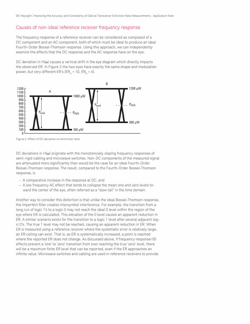
DC deviation in H(ω) causes a vertical shift in the eye diagram which directly impacts the observed ER. In Figure 2 the two eyes have exactly the same shape and modulation power, but very different ER’s (ERA = 10, ERB = 4).

DC deviations in H(ω) originate with the monotonically sloping frequency responses of semi-rigid cabling and microwave switches. Non-DC components of the measured signal are attenuated more significantly than would be the case for an ideal Fourth-Order Bessel-Thomson response. The result, compared to the Fourth-Order Bessel-Thomson response, is

– A comparative increase in the response at DC, and – A low frequency AC effect that tends to collapse the mean one and zero levels to-

ward the center of the eye, often referred as a “slow tail” in the time domain.

Another way to consider this distortion is that unlike the ideal Bessel-Thomson response, the imperfect filter creates intersymbol interference. For example, the transition from a long run of logic 1’s to a logic 0 may not reach the ideal 0 level within the region of the eye where ER is calculated. This elevation of the 0 level causes an apparent reduction in ER. A similar scenario exists for the transition to a logic 1 level after several adjacent log-ic 0’s. The true 1 level may not be reached, causing an apparent reduction in ER. When ER is measured using a reference receiver where the systematic error is relatively large, an ER ceiling can exist. That is, as ER is systematically increased, a point is reached where the reported ER does not change. As discussed above, if frequency response/ISI effects prevent a `one’ to `zero’ transition from ever reaching the true `zero’ level, there will be a maximum finite ER level that can be reported, even if the ER approaches an infinite value. Microwave switches and cabling are used in reference receivers to provide

Figure 2. Effect of DC deviation on extinction ratio

A

Pmod PAVG

Pmod

100 µW

300 µW

PAVG

B

1000 µW

1200 µW120011001000900800700600500400300200100

0


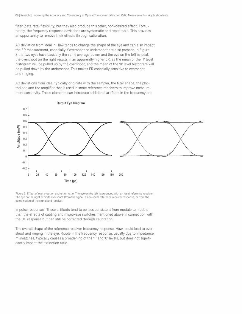
Figure 3. Effect of overshoot on extinction ratio. The eye on the left is produced with an ideal reference receiver. The eye on the right exhibits overshoot (from the signal, a non-ideal reference receiver response, or from the combination of the signal and receiver.

Output Eye Diagram

Ampli

tude

(mW

)

0.7

0.6

0.5

0.4

0.4

0.3

0.2

0.1

0

–0.1

–0.2

0 20 40 60 80 100 120 140 160 180 200

Time (ps)

filter (data rate) flexibility, but they also produce this other, non-desired effect. Fortu-nately, the frequency response deviations are systematic and repeatable. This provides an opportunity to remove their effects through calibration.

AC deviation from ideal in H(ω) tends to change the shape of the eye and can also impact the ER measurement, especially if overshoot or undershoot are also present. In Figure 3 the two eyes have basically the same average power and the eye on the left is ideal; the overshoot on the right results in an apparently higher ER, as the mean of the ‘1’ level histogram will be pulled up by the overshoot, and the mean of the ‘0’ level histogram will be pulled down by the undershoot. This makes ER especially sensitive to overshoot and ringing.

AC deviations from ideal typically originate with the sampler, the filter shape, the pho-todiode and the amplifier that is used in some reference receivers to improve measure-ment sensitivity. These elements can introduce additional artifacts in the frequency and

impulse responses. These artifacts tend to be less consistent from module to module than the effects of cabling and microwave switches mentioned above in connection with the DC response but can still be corrected through calibration.

The overall shape of the reference receiver frequency response, H(ω), could lead to over-shoot and ringing in the eye. Ripple in the frequency response, usually due to impedance mismatches, typically causes a broadening of the ‘1’ and ‘0’ levels, but does not signifi-cantly impact the extinction ratio.


Compensating for Non-Ideal Reference Receiver Frequency Response

Systematic measurement errors are those that are consistent and repeatable for specific measurement conditions. When a given signal is presented to a reference receiver that has a non-ideal frequency response, the resulting waveform is due to the convolution of the temporal reference receiver response and the waveform being measured. As discussed above, the resulting ER measurement may deviate from the ideal. However, deviation from ideal due to reference receiver frequency response is generally consistent and repeatable. If the impact of this measurement error can be determined, it can be removed from the test result. For ER measurements, this is implemented through the use of an extinction ratio correction factor (ERCF). An ERCF (positive or negative) can be determined and added to the imperfectly measured ER value. Determining the ER Cor-rection Factor is complicated by the fact that no internationally recognized calibration standards for ER exist. However, several methods are available to determine the correc-tion factor. The three methods covered in this application note are:

– Simulation – Direct measurement – Transfer standard

Simulation

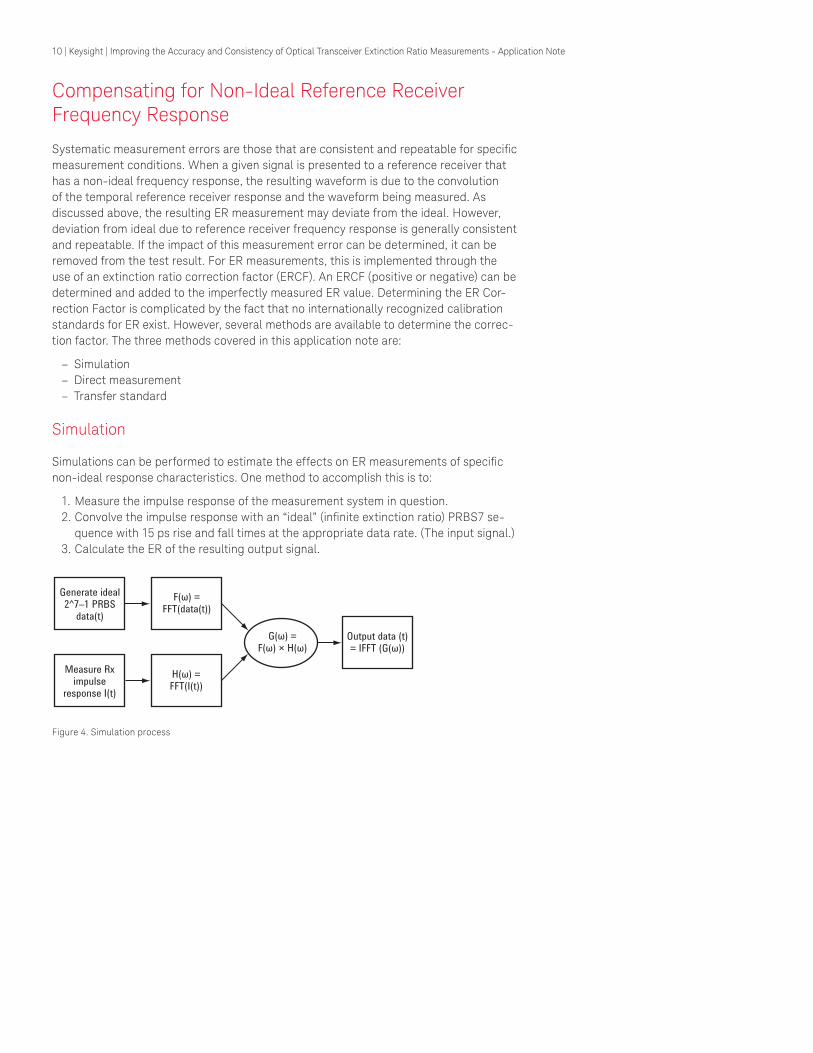
Simulations can be performed to estimate the effects on ER measurements of specific non-ideal response characteristics. One method to accomplish this is to:

1. Measure the impulse response of the measurement system in question.2. Convolve the impulse response with an “ideal” (infinite extinction ratio) PRBS7 se-

quence with 15 ps rise and fall times at the appropriate data rate. (The input signal.)3. Calculate the ER of the resulting output signal.

Generate ideal2^7–1 PRBS

data(t)

G(ω) =F(ω) × H(ω)

F(ω) =FFT(data(t))

H(ω) =FFT(I(t))

Output data (t)= IFFT (G(ω))

Measure Rximpulse

response I(t)

Figure 4. Simulation process


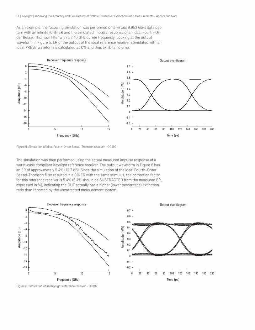
As an example, the following simulation was performed on a virtual 9.953 Gb/s data pat-tern with an infinite (0 %) ER and the simulated impulse response of an ideal Fourth-Or-der Bessel-Thomson filter with a 7.46 GHz corner frequency. Looking at the output waveform in Figure 5, ER of the output of the ideal reference receiver stimulated with an ideal PRBS7 waveform is calculated as 0% and thus exhibits no error.

The simulation was then performed using the actual measured impulse response of a worst-case compliant Keysight reference receiver. The output waveform in Figure 6 has an ER of approximately 5.4% (12.7 dB). Since the simulation of the ideal Fourth-Order Bessel-Thomson filter resulted in a 0% ER with the same stimulus, the correction factor for this reference receiver is 5.4% (5.4% should be SUBTRACTED from the measured ER, expressed in %), indicating the DUT actually has a higher (lower percentage) extinction ratio than reported by the uncorrected measurement system.

Figure 5. Simulation of ideal Fourth-Order Bessel-Thomson receiver - OC192

Figure 6. Simulation of an Keysight reference receiver - OC192

Output eye diagram

Ampli

tude

(mW

)

0.7

0.6

0.5

0.4

0.4

0.3

0.2

0.1

0

–0.1

–0.2

0 20 40 60 80 100 120 140 160 180 200

Time (ps)

Receiver frequency response

Ampli

tude

(dB)

Frequency (GHz)

0

–2

–4

–6

–8

–10

–12

–14

–16

–18

0 5 10 15

Output eye diagram

Ampli

tude

(mW

)

0.7

0.6

0.5

0.4

0.4

0.3

0.2

0.1

0

–0.1

–0.2

0 20 40 60 80 100 120 140 160 180 200

Time (ps)

Receiver frequency response

Ampl

itude

(dB)

Frequency (GHz)

0

–2

–4

–6

–8

–10

–12

–14

–16

–18

0 5 10 15


A few key points apparent from simulations of non-ideal (yet compliant) frequency response deviations performed at Keysight are:

– Low frequency phenomena primarily create an amplitude offset of the eye diagram. – Mid band (around corner frequency fc) phenomena cause significant pattern-depen-

dent jitter, and multi-level eyes that exhibit overshoot and undershoot. – High band (> fc) phenomena have less effect on the eye shape and position.

Direct measurement

Another approach to characterizing the accuracy of an ER measurement system is to measure an ER waveform1 with a known ER. When the ER is known, the ERCF can be de-termined from comparing the measured value to the actual value. When ER is expressed as a percentage, the ERCF is simply the difference between the measured and the actual result. To produce the true value, the ERCF is simply subtracted from the uncorrected measurement. (Once the correction is performed, the ER value can be mathematically converted to a linear or decibel value. This is done automatically in the 86100C).

Ideally, the reference signal will have a very high extinction ratio. Consider a test system being presented with a signal with infinite ER. When this signal is measured with an imperfect test system, a finite ER, perhaps 16 dB (or 2.5%) will be observed. The ERCF would be 2.5%. If instead, the true ER is 25 dB (0.3%), the uncorrected test system would still measure a value very close to 16 dB. If it reported 16 dB, the ERCF would be 2.2% (2.5% - 0.3%). The correction factor for the 25 ER is almost identical to the ERCF deter-mined for the infinite dB ER signal. The larger the ER is of the reference signal, the higher the confidence will be in the precision of the calculated ERCF. (In practice, sources with a stable ER in excess of 25 dB are difficult to achieve, as it can be hard to maintain align-ment of the two modulators typically used to achieve the high ER. However, as stated above, even a high ER signal with some uncertainty in the ER value can be used.)

The correction factor for a particular measurement receiver is obtained by measuring the high-ER transmitter with both the receiver under test and the 86119A (discussed below). The difference between the two measurements is the correction factor.

1. This approach is based on the paper “Accurate Optical Extinction Ratio Measurements” by Andersson and Akermark, published in ‘IEEE Photonics Technology Letters Vol 6. No 11. November 1994


Using a transfer standard

A third approach for determining an ERCF is to use a transfer standard to create a refer-ence signal with an accurately known ER. In this case, the key to obtaining an accurate ERCF value is having a measurement system that has precisely known (and compensat-ed) measurement error mechanisms, or ideally a very small measurement error. Once a signal has been characterized accurately, it can then be presented to the system being compensated. The process to derive the ERCF is the same as for the high ER signal. The ERCF is simply the difference between the measured value and the known value (when ER is expressed as a percentage).

Keysight uses a hybrid approach to determine ERCF’s for its reference receivers. An externally modulated laser source can produce an ER in the 15 to 17 dB range. The ad-vantage of this compared to the very high ER (double modulated) laser is the stability of the ER value. The actual ER is precisely determined using an 86119 optical sampling os-cilloscope. With over 800 GHz of measurement bandwidth, the error in determining the true ER of a signal is extremely low, as non-ideal frequency response errors are negligi-ble in a primarily optical measurement system. Once the true ER of the signal has been determined, this signal is then used as part of the manufacturing process to characterize 86105C reference receivers used with the 86100C Digital Communications Analyzer. Unique ERCF values are stored within the module memory for each filter setting the module supports. (Prior to December 2008, generic ERCF values were used, representa-tive of typical receiver ERCF performance).

Extinction ratio measurement variation due to source characteristics

Note that ERCF values obtained depend on the spectral characteristics of the source used to perform the calibration. Consider that the temporal waveform observed by the measurement system is the convolution of the source spectrum and the reference receiver response. As the data rate changes, so does the spectrum of the test signal. For example, as data rates are increased, the high frequency energy of the source will increase. If the reference receiver has excess loss at high frequencies (for example ISI due to skin effect loss), the waveform distortion, (mainly seen as eye closure), and the ER measurement error will be larger for the higher data rates. This implies that ERCF values generally increase as data rates increase. This is one of the reasons that there will typically be a unique ERCF for each filter setting in an 86100C optical receiver module. However, it also implies that ERCF values obtained using two sources with identical ER’s may not be identical if their spectrums vary significantly. Another viewpoint is that for a measurement receiver with a specific ERCF, two sources with different spectrums but identical ER’s may not have identical ER measurements. The ERCF process will be most accurate when the source used as a standard (or to produce a transfer standard) has a similar spectrum (but not necessarily similar ER) to the sources that will be tested with the corrected measurement system. Since this is a difficult requirement, it must be recognized as an error mechanism that is unknown but typically small for most well-be-haved laser sources. However, the ERCF process is very robust in its ability to provide consistent measurement results from system to system, independent of the test signal spectrum.


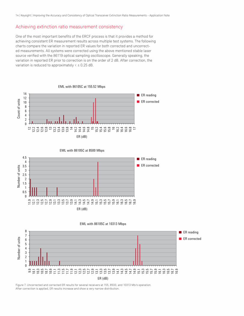
Achieving extinction ratio measurement consistency

One of the most important benefits of the ERCF process is that it provides a method for achieving consistent ER measurement results across multiple test systems. The following charts compare the variation in reported ER values for both corrected and uncorrect-ed measurements. All systems were corrected using the above mentioned stable laser source verified with the 86119 optical sampling oscilloscope. Generally speaking, the variation in reported ER prior to correction is on the order of 2 dB. After correction, the variation is reduced to approximately < ± 0.25 dB.

Figure 7. Uncorrected and corrected ER results for several receivers at 155, 8500, and 10313 Mb/s operation. After correction is applied, ER results increase and show a very narrow distribution.

14121086420

12 12.2

12.4

12.6

12.8 13 13.2

13.4

13.6

13.8 14 14.2

14.4

14.6

14.8 15 15.2

15.4

15.6

15.8 16 16.2

16.4

16.6

16.8 17

Coun

t of u

nits

ER (dB)

▀ ER reading

▀ ER corrected

EML with 86105C at 155.52 Mbps

4.54

3.53

2.52

1.51

0.50

11.9

12.1

12.3

12.5

12.7

12.9

13.1

13.3

13.5

13.7

13.9

14.1

14.3

14.5

14.7

14.9

15.1

15.3

15.5

15.7

15.9

16.1

16.3

16.5

16.7

16.9

Num

ber o

f uni

ts

ER (dB)

▀ ER reading

▀ ER corrected

EML with 86105C at 8500 Mbps

876543210

9.9 10.1

10.3

10.5

10.7

10.9

11.1

11.3

11.5

11.7

11.9 12.1

12.3

12.5

12.7

12.9

13.1

13.3

13.5

13.7

13.9

14.1

14.3

14.5

14.7

14.9

15.1

15.3

15.5

15.7

15.9

16.1

16.3

16.5

16.7

16.9

Num

ber o

f uni

ts

ER (dB)

▀ ER reading

▀ ER corrected

EML with 86105C at 10313 Mbps


It should not come as a surprise that the grouping of corrected results is very tight. After all, the ERCF process effectively forces the ER result to be the expected value. The vari-ations in measurement results are due to error mechanisms that are partially random in nature and not due to systematic errors that can be compensated by the ERCF process.

The ERCF process can also be used to enhance measurement consistency in a manufac-turing environment. Often, the key metrics used to monitor process controls in the pro-duction of high-performance laser transmitters are measurements made on the output waveforms, including ER measurements. It is common to have a ‘golden’ product (a laser that represents known, ideal performance) that can be measured on all the test systems to verify measurement consistency. This golden device can also be used as an ERCF transfer standard. If the ER of the golden laser is known (for example through measuring ER using a calibrated receiver), the laser can then be used to calibrate other test systems using the procedure below. (Note that if the golden device has a signal spectrum that is representative of most devices being tested, this technique can be used to mitigate the effects of ERCF spectrum dependence discussed above).


A transfer standard can be used to determine the extinction ratio correction factor for a particular measurement system. The steps of one example method are shown in Table 1.

Table 1.

Set up equipment

If not familiar with steps of extinction ratio measurements, review Application Note 1550-8.

Obtain a calibrated reference receiver with known extinction ratio correction factor(s). This becomes the transfer standard module.

Install the transfer standard module and the module to be calibrated for extinction ratio in the mainframe. Tighten thumb screws to hold module in place. Warm up for at least 60 minutes.

Complete module vertical calibration for both modules.

Select optical wavelength in set up for both modules.

Set measurement to capture desired number of waveforms, usually 100-2000.

Configure instrument to report ER in %.

Connect optical signal with reasonably good waveform fidelity and extinction ratio to front panel optical connector of transfer standard module.

Choose filter appropriate for rate of optical signal on both modules. Adjust vertical and horizontal scales to have one eye, centered horizontally, and covering at least one half of the vertical screen height (auto scale will normally provide this placement).

Make measurements and apply correction

Assume correction factor for transfer standard module is 4.5% for this example.

Perform extinction ratio calibration on the transfer stan-dard module.

Measure extinction ratio on the transfer standard module and record current value (called uncorrected value) after desired number of waveforms has been captured.

Uncorrected value is 21.3%

Apply the known correction factor to the uncorrected value of extinction ratio. This can be accomplished in one of two ways:Enter and apply correction factor as shown in the module in next section, orSubtract correction factor from uncorrected value and record.

Extinction ratio of measured signal is 21.3% minus 4.5%, or 16.8% (ER[corr] in Appendix A)

Perform extinction ratio calibration on the module to be calibrated.

Measure extinction ratio and record current value after desired number of waveforms has been captured.

Measured value is 22.3% (ER[meas] in Appendix A)

Determine correction factor for module of interest by subtracting extinction ratio of corrected signal on transfer standard from measured value.

Correction factor is 22.3% minus 16.8%, or 5.5% (ER[CF] in Appendix A)

Apply the correction factor into module of interest and turn on correction factor.

5.5%


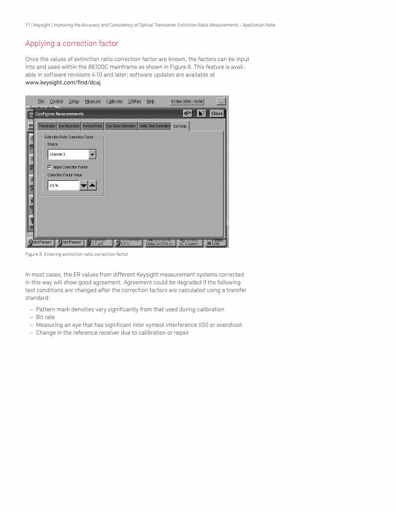
Figure 8. Entering extinction ratio correction factor

Applying a correction factor

Once the values of extinction ratio correction factor are known, the factors can be input into and used within the 86100C mainframe as shown in Figure 8. This feature is avail-able in software revisions 4.10 and later; software updates are available at www.keysight.com/find/dcaj

In most cases, the ER values from different Keysight measurement systems corrected in this way will show good agreement. Agreement could be degraded if the following test conditions are changed after the correction factors are calculated using a transfer standard:

– Pattern mark densities vary significantly from that used during calibration – Bit rate – Measuring an eye that has significant inter symbol interference (ISI) or overshoot – Change in the reference receiver due to calibration or repair


www.keysight.com/find/dcaj

Considerations when high correction factors are used with high extinction ratio signals

When ER is measured using a reference receiver where the systematic error is rela-tively large, an ER ceiling can exist. That is, as ER is systematically increased, a point is reached where the reported ER does not change. As discussed above, if frequency response/ISI effects prevent a ‘one’ to ‘zero’ transition from ever reaching the true ‘zero’ level, there will be a maximum finite ER level that can be reported, even if the ER ap-proaches an infinite value.

Figure 9 shows the ER that would be reported by a receiver with an ERCF of 4 (4%) when the ERCF process is disabled. This indicates that when the ERCF is not used, as the actual ER increases, a maximum uncorrected ER value is asymptotically approached. In this case, even as the ER becomes infinite, the maximum reported ER will not exceed ap-proximately 14 dB. For lower ERCF’s this ER ceiling is higher, for higher ERCF’s the ceiling is decreased. There will be no ceiling when ERCF is 0.

Figure 9. A reference receiver with a large ERCF will exhibit a ceiling in uncorrected ER

1514131211109876543

Repo

rted

unco

rrect

ed E

R (E

RCF =

4)

Actual ER3 4 5 6 7 8 9 10 11 12 13 14 15 16 17 18 19 20 21 22 23 24 25 26


An ER ceiling can be corrected through the ERCF process. However, from the perspec-tive of measurement consistency, some troublesome results can occur. The following table shows the corrected ER versus the uncorrected ER for a variety of ERCF values. For example, if the uncorrected ER measurement is 11 dB, and the receiver ERCF is 2 (2%), the corrected (true) ER is slightly above 12 dB. The ‘correction’ is significant, but not severe.

If the ERCF is large, for example 4, and the measured ER is also large, for example 13.4 dB, two important effects are observed. The corrected ER is 22 dB, representing a dramatic change from the uncorrected value. There is also the potential for very wide variation in the corrected ER value. Recall that the ERCF process is capable of eliminating the sys-tematic ER measurement error due to frequency response. Other measurement errors are not removed, including random error mechanisms. Any fluctuation in the uncor-rected ER results in a much larger fluctuations in the corrected ER. If the uncorrected ER varies from 13.2 to 13.6 dB, the corrected ER will vary from 21 to almost 24.5 dB for a 4.0 ERCF. A ± 0.2 dB fluctuation is amplified to a –1 to +2.5 dB variance in reported values. While the corrected values are likely much closer to the true ER value than the uncorrected results, the wide fluctuation can erode confidence in the instrumentation and present difficulties in manufacturing environments that use ER results to gauge pro-cess control. (On the other hand, when ER values are in the 11 dB (uncorrected range) and the ERCF is 2, a ± 0.2 variation in the raw ER measurement translates to a ± 0.25 dB variation. Amplification of the measurement variance is negligible).

Figure 10. Corrected versus uncorrected ER for various ERCF values

22

17

12

7

22 3 4 5 6 7 8 9

Measured ER10 11 12 13 14 15 16

Corre

cted

ER

▀ ERCF = 7

▀ ERCF = 6

▀ ERCF = 5

▀ ERCF = 4

▀ ERCF = 3

▀ ERCF = 2

▀ ERCF = 1

▀ ERCF = 0


While an ER result of 24.5 dB represents a large difference from 13.4 or even 21 dB, the actual difference in transmitter performance and its usability in a communications sys-tem is quite subtle. While the ERCF alters the ER value as much as 11 dB, for a fixed one level, the modulation amplitude (difference between the one and zero levels) and even the average power differences are hardly noticeable at less than 0.2 dB.

The benefit of achieving very high ER results, facilitated through a large ERCF, can easily be lost in the measurement variation that may accompany it. Thus the implementation of ERCF’s is adjusted to provide a good trade off between accuracy and stability. For ERCF values in excess of 1%, the ERCF value automatically implemented in the calibra-tion process of 86105C reference receivers is reduced by 1%. For example, if the ERCF is measured to be 4.5%, a value of 3.5% is used. If the ERCF is determined to be 1% or less, the ERCF is set to 0 (no correction is performed).

If it is desirable to measure very high extinction ratios with the highest accuracy, and an increase in measurement variation is tolerable, it is easy to override the stored ERCF value. Simply add 1% to the installed value. If the installed ERCF is less than 1, it is rec-ommended that no ERCF be used.

It is important to note again that when ER values are in typical ranges of 8 to 10 dB, the ‘instability magnification’ phenomenon is small. In addition, the difference in corrected ER for a variation in ERCF is also small. Referring to figure 10 above, if the uncorrected ER is 10 dB, an ERCF of 3 will report a corrected ER of about 11.5 dB, while the ‘padded’ ERCF of 2 will report 11.0 dB. The 1% ERCF reduction provides a small guard band for typical ER testing as well as increased stability when making high ER measurements.


Summary and Conclusions

Extinction ratio, especially at high values, continues to be a challenging measurement to make. Measurement accuracy and measurement repeatability from system to system remain as industry concerns.

Factors that can degrade the accuracy of an extinction ratio measurement are:

– Shape and frequency content of input waveform – Offsets generated by the instrumentation – Measurement uncertainty in determining the amplitudes of the waveform – Non-ideal frequency response of the instrumentation

Although there is no traceable standard for extinction ratio that will enable the industry to fully compensate for these issues, Keysight has taken several steps to enhance accu-racy and repeatability:

– The Keysight 86100 DCA uses an extinction ratio calibration process to compensate for offsets generated by the instrumentation

– The methods described in this paper explain how to determine ER correction factors that help compensate for the non-ideal frequency response of the instrumentation.

By using the methods described in this paper to determine extinction ratio correction factors, the user can both decrease the uncertainty in the measurement and improve repeatability from system to system. Based on the causes of the ER inaccuracies the correction factor is compensating for (DC effects, AC effects or both), a correction factor may be applicable to a specific measurement system or a family of measure-ment systems.

Our experience in determining correction factors has shown they are dependent on bit rate, type of pattern, and frequency content, with the most significant variable being bit rate (e.g. OC-48 versus OC-192). For the most accurate extinction ratio measurement results, the appropriate filter should be used for the pattern and the correction factor for any particular measurement system should be determined for the specific bit rate and pattern of interest.

Keysight has determined extinction ratio correction factors for common reference receiv-ers and these are available in Appendix A.


APPENDIX A

Use of reference receiver correction factors

Keysight modules closely match the response of an ideal Fourth-Order Bessel-Thomson response. Some DC characteristics cause them to understate extinction ratio, particular-ly for receiver configurations, which may have significant internal cabling associated with multiple physical switches and filters.

The very consistent nature of the response of the Keysight modules and their well behaved AC characteristics allow an extinction ratio correction factor approach to be effective across the product family, by configuration and bit rate. Keysight has measured the 86105B and 86105C modules for the appropriate extinction ratio correction factor and offers these nominal correction factors to provide extinction ratio measurements with the best correlation to an ideal Fourth-Order Bessel-Thomson.

Testing was done to determine the impact of PRBS pattern length, from PRBS7 to PRBS31, on the correction factors. The variation across various length PRBS sequences is negligible. Non-PRBS data with specific spectral characteristics may behave different-ly and should be compared against PRBS data for verification. However, the consistency across different PRBS patterns gives reasonable confidence that any differences should be small.

Recommended correction factors

The correction factors listed here are typically worst-case (conservative ERCF values that result in a lower severity correction) for the product model number. 86105C receiv-ers produced after December 2008 are individually characterized and will have larger ERCF values than those listed here.

Table 2.

86105B 86105C

Designations Data rates (Gb/s)

Option 101

Options 102/103

Options 100/300

Option 200

OC-3/STM-1 0.155 N/A 0.5% 0.5% N/A

OC-12/STM-4 0.622 N/A 0.5% 0.8% N/A

1x Fibre Channel 1.063 N/A 0.7% 2.5% N/A

Gigabit Ethernet 1.250 N/A 0.9% 1.3% N/A


OC-48/STM-16 2.488 N/A 2.3% 2.0% N/A

2 Gb Ethernet 2.500

OC-48/STM-16 FEC 2.666 N/A 3.2% 2.0% N/A

10 Gb Ethernet LX-4 3.125 N/A 3.4% 3.3% N/A


OC-192/STM-64 9.953

2.8% 4.5%

4.0% 1.5%

10 Gb Ethernet 10.312

10x Fibre Channel 10.519

OC-192/STM-64 FEC 10.664

OC-192/STM-64 FEC 10.709

10 Gb Ethernet FEC 11.096 N/A N/A

10x Fibre Channel FEC 11.317 N/A N/A


As of January, 2009, unique correction factors are determined for every filter setting of every 86105C as part of the standard manufacturing process. The recommended correc-tion factors for the 86105C are loaded into the module memory. The appropriate value for each rate is placed into the correction factor dialog box as a recommended value, and is based on the filter selected. Users choose to turn on the recommended value or override these values with ones that they have determined for their specific measure-ment module. Currently, unique correction factors are not available for the 86105B and the values from the table above should be used. A manufacturing calibration process is being considered for the 86105B. Contact your local Keysight representative for the latest details.

Using the correction factors

Extinction ratio can be expressed in terms of percentages, decibels, or linear ratios. This description uses extinction ratio expressed in % because this form provides the quickest application of correction factor. To convert an ER measurement from % to dB or from dB to % you can use the following equations:

ER% =100*1/(10^(ERdB/10))ERdB = 10*log10(1/(ER%/100))

To obtain the corrected extinction ratio measurement, subtract the correction factor from the measured extinction ratio expressed in percentage. If the correction factor is entered into the 86100C and the correction factor is enabled, then the measured value is automatically adjusted. As an example, typical measured and corrected extinction ratio values are given in Table 3 for a correction factor of 4%, which is a common value at higher data rates.


These values are derived using this formula:

ER[corr] = ER[meas] – 10*log10 {1 - ER[CF] * 10 ^ (ER[meas] /10) }Where:

ER[corr] = value in dB adjusted for ER correction factorER[meas] = value in dB measured on digital communications analyzerER[CF] = ER correction factor in %, which comes from table above, from memory in 86105C module, or provided by the user

Table 3. Look-up table for corrected extinction ratios

Measured extinction ratio Correction factor Corrected extinction ratio

dB Linear Percentage Percentage Linear dB

3 2.0 50.1%

4.0%

46.1% 2.2 3.4

4 2.5 39.8% 35.8% 2.8 4.5

5 3.2 31.6% 27.6% 3.6 5.6

6 4.0 25.1% 21.1% 4.7 6.8

7 5.0 20.0% 16.0% 6.3 8.0

8 6.3 15.8% 11.8% 8.4 9.3

9 7.9 12.6% 8.6% 11.6 10.7

10 10.0 10.0% 6.0% 16.7 12.2

11 12.6 7.9% 3.9% 25.4 14.0

12 15.8 6.3% 2.3% 43.3 16.4

13 20.0 5.0% 1.0% 98.8 19.9



This information is subject to change without notice.© Keysight Technologies, 2017Published in USA, December 1, 20175989-2602ENwww.keysight.com

This document was previously known as Application Note 1550-9

For more information on Keysight Technologies’ products, applications or services, please contact your local Keysight office. The complete list is available at:www.keysight.com/find/contactus

Americas Canada (877) 894 4414Brazil 55 11 3351 7010Mexico 001 800 254 2440United States (800) 829 4444

Asia PacificAustralia 1 800 629 485China 800 810 0189Hong Kong 800 938 693India 1 800 11 2626Japan 0120 (421) 345Korea 080 769 0800Malaysia 1 800 888 848Singapore 1 800 375 8100Taiwan 0800 047 866Other AP Countries (65) 6375 8100

Europe & Middle EastAustria 0800 001122Belgium 0800 58580Finland 0800 523252France 0805 980333Germany 0800 6270999Ireland 1800 832700Israel 1 809 343051Italy 800 599100Luxembourg +32 800 58580Netherlands 0800 0233200Russia 8800 5009286Spain 800 000154Sweden 0200 882255Switzerland 0800 805353

Opt. 1 (DE)Opt. 2 (FR)Opt. 3 (IT)

United Kingdom 0800 0260637

For other unlisted countries:www.keysight.com/find/contactus(BP-9-7-17)

DEKRA CertifiedISO9001 Quality Management System

www.keysight.com/go/qualityKeysight Technologies, Inc.DEKRA Certified ISO 9001:2015Quality Management System

Evolving Since 1939Our unique combination of hardware, software, services, and people can help you reach your next breakthrough. We are unlocking the future of technology. From Hewlett-Packard to Agilent to Keysight.

myKeysightwww.keysight.com/find/mykeysightA personalized view into the information most relevant to you.

http://www.keysight.com/find/emt_product_registrationRegister your products to get up-to-date product information and find warranty information.

Keysight Serviceswww.keysight.com/find/serviceKeysight Services can help from acquisition to renewal across your instrument’s lifecycle. Our comprehensive service offerings—one-stop calibration, repair, asset management, technology refresh, consulting, training and more—helps you improve product quality and lower costs.

Keysight Assurance Planswww.keysight.com/find/AssurancePlansUp to ten years of protection and no budgetary surprises to ensure your instruments are operating to specification, so you can rely on accurate measurements.

Keysight Channel Partnerswww.keysight.com/find/channelpartnersGet the best of both worlds: Keysight’s measurement expertise and product breadth, combined with channel partner convenience.

http://www.keysight.com

http://www.keysight.com/find/contactus

http://www.keysight.com/find/contactus

http://www.keysight.com/go/quality

http://www.keysight.com/find/mykeysight

http://www.keysight.com/find/emt_product_registration

http://www.keysight.com/find/service

http://www.keysight.com/find/AssurancePlans

http://www.keysight.com/find/channelpartners

keysight technologies improving the accuracy and...

Documents