Kinematics and Dynamic Modeling of a Planar Hydraulic ElastomerActuator

Mahdi Momeni Kelageri, Mikko Heikkila, Jarno Jokinen, Matti Linjama, Reza Ghabcheloo1

Abstract— This paper presents modeling of a compliant2D manipulator, a so called soft hydraulic/fluidic elastomeractuator. Our focus is on fiber-Reinforced Fluidic ElastomerActuators (RFEA) driven by a constant pressure hydraulicsupply and modulated on/off valves. We present a model thatnot only provides the dynamics behavior of the system but alsothe kinematics of the actuator. In addition to that, the relationbetween the applied hydraulic pressure and the bending angleof the soft actuator and thus, its tip position is formulated ina systematic way. We also present a steady state model thatcalculates the bending angle given the fluid pressure which canbe beneficial to find out the initial values of the parametersduring the system identification process. Our experimentalresults verify and validate the performance of the proposedmodeling approach both in transition and steady states. Due toits inherent simplicity, this model shall also be used in real-timecontrol of the soft actuators.

I. INTRODUCTION

Biology has long been an important source of inspira-tion for the engineers in order to make ever-more capablemachines. Of noticeable features exploited from biologicalsystems is softness and body compliance which tend toseek simplicity in interaction of such systems with theirenvironment. Several of the lessons learned from studyingbiological systems are now culminating in the definition ofa new class of machines that is referred to as soft robots[1]. Soft material actuators are made of deformable materialswhich means that, theoretically, the actuator tip can attainevery point in 3D workspace with an infinite number ofconfigurations.

To improve the performance of a system, its behavior hasto be modeled more accurately. Furthermore, the possibilityto calculate the dynamic model in real-time is required forcontrol algorithms. Soft material actuators, in particular, canpotentially undergo large deformations which turns them tosomehow complex systems which are not straightforward toacceptably accurately model.

A. Prior Work

The majority of works in modeling of soft robots deal withthe kinematics of the system. Not many works have beenpresented on dynamic modeling of the system. There are alsosome works on modeling of soft robots using finite elementsmethod (FEM). To the best of our knowledge, there is nowork incorporating both kinematics and dynamics models at

*This work was supported by Academy of Finland under the ActiveFitproject (No. 295817)

1Authors are with Tampere University of Technology, Tampere,Finland {mahdi.momenikelageri, mikko.heikkila,matti.linjama, reza.ghabcheloo}@tut.fi

(a) test system (b) schematic diagram

Fig. 1: Digital hydraulic drive system for controlling a softactuator

the same time, which is also fast enough to be implementedin real-time control applications. In this section we willbriefly review some of the most important prior works.

In [2] the authors develop a continuum kinematics for anelephant trunk and demonstrate how it can be used in obsta-cle avoidance. In [3] a kinematic algorithm for controlling theshape of multi-segment continuum manipulators is presented.Despite numerous continuum manipulator designs, it is oftenpossible to find out their kinematics based on a piece-wiseconstant curvature (PCC) model [4]. However, there aretwo important, somehow related, issues with PCC modelsthat can seriously influence on its accuracy and restrict itsapplication: 1) when the deformation is large, and 2) thedeformation is not according to the PCC assumption in allsoft material actuators. For this reason, the authors in [5]developed general variable curvature continuum kinematics.

One common approach to shape estimation in continuumrobots is measuring strain along the manipulator axis [6],[7] and applying dynamical models of the manipulator inorder to predict the curvature of the manipulator basedon measured strain. Another method for shape estimationis using fiber optic sensors along the body. This method,however, suffers from propagation losses when they arebent [8]. In [9] the authors use vision system to estimatethe curvature. Vision systems are usually based on PCCassumptions that can be inaccurate if large deformation andgravitational loading effects are present. In [10] the authorspresent three different methods of shape estimation based ongeometrically exact mechanical model which are: 1) a loadcell mounted at the base of the manipulator 2) using cableencoders running through the length of the actuator and 3)using inclinometers mounted at the end of each section ofthe manipulator.

Dynamic modeling of soft material actuators capable ofapplying to real-time control is a very complex task and

arX

iv:1

806.

0490

7v1

[cs

.RO

] 1

3 Ju

n 20

18

thus, most papers in the field treat the control problemfrom the kinematic point of view. The dynamic modelingof extensible soft elastomer actuators is an important openresearch field. In [11] a dynamic model for hyper-redundantstructure as an infinite degree of freedom continuum modelis proposed. In [12] the authors presented dynamic model foran eel-like robot. The authors in [13] represent a dynamicmodel for an extensible tentacle arm. However, their modelis derived based on the restrictive assumption that the armdoesn’t bend past a small-strain region, where linear stress-strain are obeyd and permanent deformation does not exist. Athree-dimensional dynamic model is presented in [14] for aninextensible continuum manipulator based on the assumptionthat the continuum robot is a combination of rigid slices.The dynamic model is then derived by obtaining the limitof serial rigid chain model as the degree of freedom goesto infinity. Further, the authors in [15] extend the modelto include the extensible continuum manipulator. However,they work applies to the continuum manipulator with notorsional effect. Besides, there is no comparison betweenthe simulation results and the experimental measurementsin order for the model to be evaluated.

Another approach for modeling soft actuators is a commonnumerical method for solving engineering problems, i.e.,Finite Element Method (FEM). However, the design processof a rubber actuator is difficult because of large deformationand material nonlinearity. One of the FEM advantages is itscapability for taking into account nonlinearities [16] causedby material, large deformation or contact. Typically, analysisof soft material actuators have limited to small strains andlinear material behaviour [17]. Usage of three-dimensionalsolid elements allows modelling three-dimensional deforma-tion of the actuator, which can be used in the optimizationof the actuator cross-section, for example [18]. Non-linearFEM is an effective method for design process [19]. Thedisadvantage of the solid FEM model is the large numberof solvable parameters, which increases analysis time. As amatter of fact, the main benefits of FEM modeling lies indesign process and they are not very useful for real-timecontrol applications.

B. Contributions

In this paper, we present an approach for kinematics anddynamic modeling of Reinforced Fluidic Elastomer Actuator(RFEA) taking advantage of the revolute spring-damperactuators and Lagrangian equations. Closest work to ourpaper is a quite recent paper [20], where they model a softactuator using series of lines connected with viscoelasticjoints. They assume that the applied torque is simply a linearfunction of applied pressure, i.e., τi(P) = αiP and αi to beidentified. They generally develop their work based on thisto be identified equation. Whereas in our work, we derive theequations based on system parameters which gives a betterinsight to the idea of modeling. Our equations agree withand validate some of the assumptions in [20]. Furthermore,we present a steady state model which acceptably accuratelyprovides the bending angle (and thus the kinematics) of the

Fig. 2: Experimental Setup

actuator given the physical values of the actuator. This steadystate model is also beneficial for identifying the unknownparameters. More specifically, this paper contributes thefollowing:• An analytical formulation for dynamic and kinematics

modeling of RFEA based on Lagrange equations. Thismodel not only provides the dynamic behavior of thesystem but also the kinematics of the elastomer actuator,given the applied pressure as the input to the system;

• Presenting a novel and acceptably accurate steady statemodel which relates the bending angle to the inner/outertube diameter and the fluid pressure. The model is usedduring identification of the dynamic model’s parameter;

• Investigation of the impact of the number of degrees offreedom on the proposed model;

• Extensive experiments for validation of the model.

II. SYSTEM DESCRIPTION

The hydraulic elastomer actuator system studied in this pa-per is composed of: A) a soft and compliant fiber-reinforcedone-directional elastomer tube (outer radius ro = 8mm, innerradius ri = 6 mm, length L = 155 mm) B) digital hydraulicdrive system, C) vision system used for model verificationand identification, Fig. 1 and Fig. 2, and D) control hardware.We will next describe these elements:

A. Elastomer Actuator

For satisfying the research requirements of this work, theactuator was designed with a cylindrical shape, as shownin Fig. 2, and made of polydimethylosiloxane (PDMS).The number of turns of fibers was set to 240 as it gavethe highest force output as well as bending angle, Fig. 3[21]. Bending principle is based on asymmetric structureand expansion in the direction of the lowest modulus bypressurizing or depressurizing internal fluid which inducesstress in elastomer. In this work, the actuator’s workspace isconstrained to X-Y plane while it is only capable of one-directional bending.

B. Digital Hydraulic Drive

A digital hydraulic drive system is used to control theRFEA. The test system is shown in Fig. 1a while thecorresponding hydraulic diagram is depicted in Fig. 1b: Thesize of the tank 1 is 0.6 l and it is connected to the diaphragmpump 2. The pump is then connected to a 12 V DC motor

Fig. 3: The effect of number of turns on actuation perfor-mance of PDMS at 5 KPa

3 having a maximum power of 36 W. The maximum flowrate of the hydraulic power unit 2 is 3.6 l/min whereas themaximum system pressure is limited to about 600 kPa bythe pressure switch 4. The hydro-pneumatic accumulator 5is attached to the supply line to store the hydraulic energy.The fluid volume in the actuator port 8 can be increasedby opening the high-pressure valve 6. On the other hand,opening the low-pressure valve 7 decreases the actuator fluidvolume as the flow direction is towards the tank. The orificediameter of these on/off valves is 1 mm. Water is used asthe hydraulic medium in the drive system.

C. Vision System

To verify the simulation results, a GoPro camera has beenused in order to find out the curvature/bending angle ofthe manipulator and localize the tip offline. The resolutionand the frame per seconds (FPS) of the camera is set to720×1280 and 240 respectively, while MATLAB Image Pro-cessing and Computer Vision Toolboxes have been used fortip localization and curvature estimation. The camera is alsocalibrated at the initialization time before the experiment.

D. Control Hardware

A dSPACE DS1006 Processor Board is utilized to runpressure control algorithms of the test system. Valve controlcommands are executed using DS4004 Digital I/O Boardwhile the hydraulic pressure in the actuator is measured usingDS2003 A/D board. The pressure data is then recorded in adatabase to be used for verification of the model.

III. MODELING

In this section, we derive the equations for the completerepresentation of the kinematics and dynamics behavior ofthe RFEA. Our goal is to derive the bending angle andtip position in a closed form equation given the physicalcharacteristics of the actuator, i.e., inner radius ri, outerradius ro, actuator’s length l, and fluid pressure phyd . Fig. 4shows the overal system including the hydraulic drive systemand the segmented elastomer actuator, while Fig. 5 showsthe schematic of the hydraulic system in more details. Itshould be noted that modeling the hydraulic drive system is

Fig. 4: Modeled system

out of the scope of this paper. We will eventually verify themodel both in simulation and experimentally and comparethe results. The following assumptions are valid in this work:• Assumption 1: The RFEA is moving freely in 2D planar

surface, i.e., it does not collide with an obstacle in itsworkspace nor it is carrying a payload.

• Assumption 2: The fibers are inextensible enough andprevent the actuator to radially expand. As a matter offact, the outer radius of the actuator is assumed to beconstant when the tube is pressurized.

• Assumption 3: The tube is made of material which hasbulk modulus of about 2 GPa. The tube, therefore, isassumed to be incompressible.

• Assumption 4: The material volume, Vrubber is constant.• Assumption 5: For simplicity, it is assumed that the

RFEA is made of uniformly distributed material.

A. Soft Actuator Modeling

The main idea behind modeling the RFEA comes from theconventional mass-spring-damper system. That is to say, inorder to find the dynamic and kinematics model of the RFEA,it is considered as a multibody system composed of n mass-spring-damper system. However, since the actuator is a one-directional bending type, the mass-spring-damper system isconstrained with a revolute joint to represent the inextensibleside of the tube, a so called Revolute Spring DamperActuator (RSDA), while the other free (unconstrained) siderepresents the extensible side of the soft actuator, as shown inFig. 5. Furthermore, based on assumption 5, it is reasonableto consider the tube as a combination of equi-length bodies.In this case, we can write: ∆L = L

n , where L is the length ofthe tube and n is the number of segments (bodies). We willcall n as the number of Degrees of Freedom (n-DoF).

We will start by modeling the soft material actuator usingLagrange equations. We will also consider the inner radiusri, fluid volume Vseg, and the fluid pressure phyd , and thusthe acting force/torque, as time dependent parameters andinclude their instantaneous values which contribute in modelaccuracy.

Fig. 5: Mass-spring-damper system constrained with a revo-lute joint

1) Instantaneous Inner Radius: The inner radius of thetube can be calculated according to the corresponding anglebetween the two adjacent RSDA body in the proposedmultibody system. Assuming that in the fiber reinforcedelastomer actuators the outer radius remains constant andalso the material is incompressible, we can write:

dri j

dt=

r2o− r2

i j

2(s j +L0)ri j

ds j

dt(1)

where ri, ro, s, and L0 are the tube’s inner radius, outerradius, elongation arc due to bending, and the initial lengthof the tube segment. Besides, j = 1, · · · ,n is the index ofsegments considered for modeling the tube.

2) Volume: The volume inside the tube’s jth segment,Vseg j , is calculated according to the following equation:

dVseg j

dt= πrori(ri

dθ j

dt+2θ j

dri

dt) (2)

where ro, the outer radius is constant and θ j is the anglebetween the two adjacent segment. It should also be notedthat the bending θ is the sum of the angles between thesegments, i.e.;

θ =n

∑j=1

θ j (3)

3) Acting Forces: The forces acting on the elastomer tubeare the hydraulic force generated by the fluid pressure, springforce generated by the strain (bending) and damping forcescaused by friction.

The hydraulic pressure, phyd , is supposed to be uniformlydistributed along the tube and thus, is identical for eachsegment. The axial hydraulic force, Fhyd , is calculated asfollows:

Fhyd j = πr2i j

phyd (4)

Fig. 6: A segment of the tube

and thus, the hydraulic torque applied to each joint in theRSDA multibody system becomes:

(5)τhyd j = rhydFhyd j

= phydπr2i j

rhyd

where rhyd is the effective position vector from where thehydraulic force is applied to the system, and will be identifiedduring system identification. However, if the number ofsegments in the proposed multibody system is limited, i.e.,the angle α in Fig. 6 is not negligible any more, then:

τhyd j = phydA jRcosα j (6)

where: {α = tan−1 ∆L

ro

R =√

r2o +∆L2

(7)

where ∆L is the length of each body in the RSDA multibodysystem. It may also worth noting that our experimental resultsverify that the Eq. 5 produces quite acceptable results andEq. 6 may not be really needed in practice.

To capture nonlinear mechanical behavior of the actuatormaterial and its effect on springer and damper coefficients,we have considered that the spring and damper coefficientsare changing with respect to the inner radius of the tube.Spring coefficients are, therefore, defined by:

k j = ri j mk + k0 (8)

where mk is a coefficient that its value is estimated throughsystem identification. Eq. 8 reflects the fact that as the innerradius of the tube increases (tube is stretched), materialgets less stiff (refer to the sections on experimental vali-dation/discussion and conclusion).

The damper coefficients are also calculated by:

b j =

{ri j mbpos +b0pos : dθ

dt ≥ 0

ri j mbneg +b0neg : dθ

dt < 0(9)

which also includes the direction dependency of dampingeffect and mb is a coefficient that its value is estimatedthrough system identification.

Even though the tube is made of uniformly distributedmaterial, the spring/damper coefficients are different for eachsegment as the instantaneous inner radius is not identical.However, k0, mk, b0pos , b0neg , mbpos and mbneg are supposedto be identical for each segment.

4) Steady State Formulation: Assuming the proposedmultibody system while the gravity is zero, in steady statethe torques applied to the tube are the fluid pressure torqueτhyd and the spring torque τspring. The equilibrium equationfor the torques can, therefore, be written as:

rhydFhyd = roFspring = τss⇒ rhydπr2iss phyd− kssθss = 0 (10)

where riss , θss , and τiss are the inner radius of the tube,bending angle, Eq. 3, and the torque in steady state, andkss =

k jn where k j is the coefficients in Eq. 8. The bending

angle, therefore, can be calculated as:

θss =rhydπr2

issphyd

kss(11)

We assume that the revolute joints, approximately, forman arc of a circle while bent (this is a local assumptionand not for the whole tube). Each segment’s elongations (displacement between the center of masses of adjacentbodies), therefore, can be calculated as:

s = rorhydπr2

issphyd

kss(12)

The inner radius of the tube changes as the fluid pressurechanges and so does the bending angle. Considering theassumptions of the modeling, we can write:

V = constant⇒ L0π(r2o− r2

i0) = π(L0 + s)(r2o− r2

iss) (13)

where ri0 is the initial inner radius of the tube, i.e., while thetube is unpressurized. Solving Eq. 13 for riss we will get:

riss =±

√(roθss +L0)(r3

oθss +L0r2i0)

roθss +L0(14)

where only the positive solution is acceptable. ConsideringEq. 10 and 14 we can write:

θss =rhydπ(

√(roθss+L0)(r3

oθss+L0r2i0)

roθss+L0)2 phyd

kss(15)

which is a second order equation of θss, the bending anglein steady states, and can be readily solved (only the positivesolution is acceptable). Eq. 15, obviously, presents the bend-ing angle in the steady states given the known parametersfrom the physical characteristics of the actuator.

Based on the above explanations, it is now possible toderive the kinematics and dynamic model of the RFEA(please refer to the Appendix)

IV. EXPERIMENTAL VALIDATION

In this section, we verify the performance of the proposedmodel both in simulation and experimentally. We also inves-tigate the impact of the number of degrees of freedom inthe accuracy of the proposed RSDA multibody system. Todo so, two different models have been studied :1)a 2-DoFmodel, and 2) an 8-DoF model.

The current version of the fiber-reinforced elastomer ma-nipulator used in this research work, Fig. 2, is capable ofcarrying payloads up to 30g. However, for verification andvalidation of the proposed model, the experiments are carriedout while it is unloaded. The hydraulic drive system canaccurately control the fluid pressure in real-time and movethe tip to any position in its workspace. The position ofthe tip and the bending angle are measured using an imageprocessing model implemented in MATLAB. The proposed2-DoF and 8-DoF models of the system are also implementedin MATLAB. In both models, the inner radius of the tube,the spring coefficients and the damper coefficients were sup-posed to be variable and calculated dynamically as explainedin Eq. 1, 8 and 9. In order to verify the performance of theproposed model, the parameters of the model were identified.To do so, an independent experiment has been carried outwhile the soft actuator was pressurized until 270kPa. Thetip position and the hydraulic pressure have been recordedand the tip y position has been used as a reference forparameter identification so that the simulation results fitinto the measured data. Simulink parameter estimation isused to determine the unknown model parameters shownin Table I. Initial assumptions for the parameter estimationare that the variables b0neg , b0pos, k0 are positive, whereas0.003m < rhyd < 0.005m. Furthermore, it is assumed thatthe tube becomes less stiff when it elongates (inner radiusincreases); thus, mk has to be negative. Fig. 7a and 7bshow the input fluid pressure and the corresponding tip yposition for both real system and the proposed 2-DoF and8-DoF models, respectively. Table I also shows the identifiedparameters for both models.

Even though the results of both 2-DoF and 8-DoF modelslook very promising at the first sight, their main differenceappears when the x-coordinate is considered too. Fig. 8shows the simulation results and the real path followed bythe two models. Apparently, the lower the number of degreesof freedom, the higher discrepancy between the measuredpath and the simulated one. This was already obvious andpredictable as the gravity will have different effect on themodeled system when the number of degrees of freedomchanges.

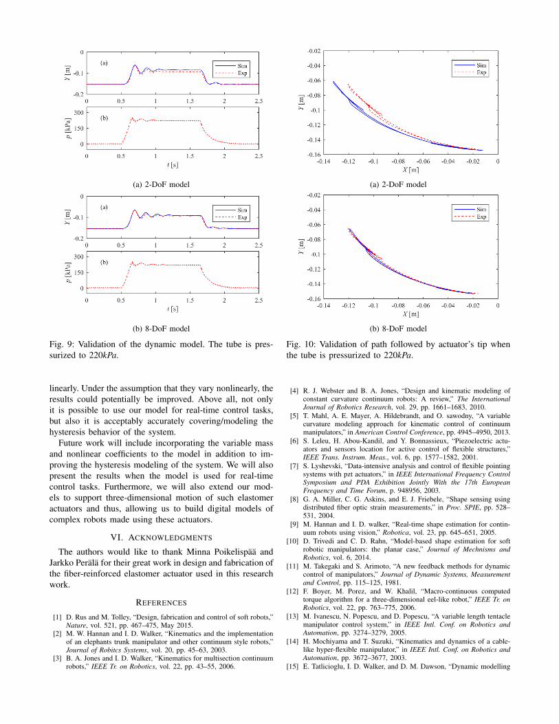
To cross validate the performance of the proposed model,series of validation experiments have been done where differ-ent fluid pressure have been fed to the soft actuator and thetip positions were measured. The same fluid pressure havealso been fed to the simulation model with the parameterspreviously identified and presented in table I. As an example,we pick the case where the tube is pressurized up to 220kPa. Fig. 9 shows the validation results for both 2-DoF and

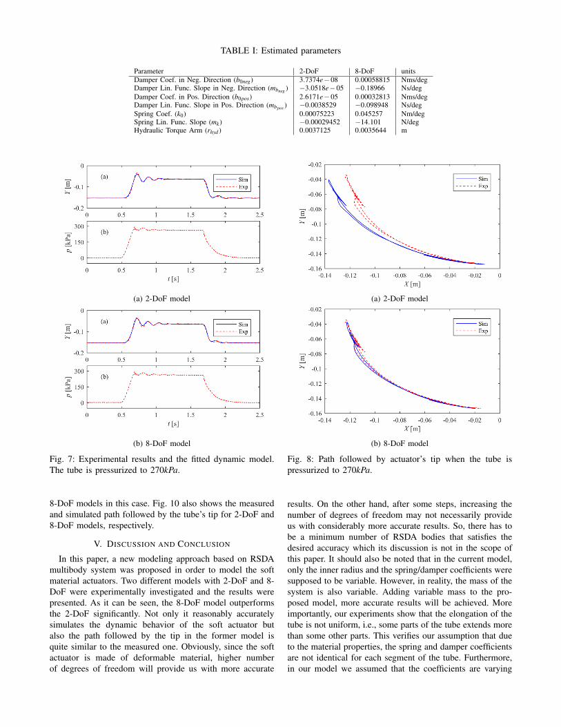
TABLE I: Estimated parameters

Parameter 2-DoF 8-DoF unitsDamper Coef. in Neg. Direction (b0neg) 3.7374e−08 0.00058815 Nms/degDamper Lin. Func. Slope in Neg. Direction (mbneg ) −3.0518e−05 −0.18966 Ns/degDamper Coef. in Pos. Direction (b0pos) 2.6171e−05 0.00032813 Nms/degDamper Lin. Func. Slope in Pos. Direction (mbpos ) −0.0038529 −0.098948 Ns/degSpring Coef. (k0) 0.00075223 0.045257 Nm/degSpring Lin. Func. Slope (mk) −0.00029452 −14.101 N/degHydraulic Torque Arm (rhyd ) 0.0037125 0.0035644 m

(a) 2-DoF model

(b) 8-DoF model

Fig. 7: Experimental results and the fitted dynamic model.The tube is pressurized to 270kPa.

8-DoF models in this case. Fig. 10 also shows the measuredand simulated path followed by the tube’s tip for 2-DoF and8-DoF models, respectively.

V. DISCUSSION AND CONCLUSION

In this paper, a new modeling approach based on RSDAmultibody system was proposed in order to model the softmaterial actuators. Two different models with 2-DoF and 8-DoF were experimentally investigated and the results werepresented. As it can be seen, the 8-DoF model outperformsthe 2-DoF significantly. Not only it reasonably accuratelysimulates the dynamic behavior of the soft actuator butalso the path followed by the tip in the former model isquite similar to the measured one. Obviously, since the softactuator is made of deformable material, higher numberof degrees of freedom will provide us with more accurate

(a) 2-DoF model

(b) 8-DoF model

Fig. 8: Path followed by actuator’s tip when the tube ispressurized to 270kPa.

results. On the other hand, after some steps, increasing thenumber of degrees of freedom may not necessarily provideus with considerably more accurate results. So, there has tobe a minimum number of RSDA bodies that satisfies thedesired accuracy which its discussion is not in the scope ofthis paper. It should also be noted that in the current model,only the inner radius and the spring/damper coefficients weresupposed to be variable. However, in reality, the mass of thesystem is also variable. Adding variable mass to the pro-posed model, more accurate results will be achieved. Moreimportantly, our experiments show that the elongation of thetube is not uniform, i.e., some parts of the tube extends morethan some other parts. This verifies our assumption that dueto the material properties, the spring and damper coefficientsare not identical for each segment of the tube. Furthermore,in our model we assumed that the coefficients are varying

(a) 2-DoF model

(b) 8-DoF model

Fig. 9: Validation of the dynamic model. The tube is pres-surized to 220kPa.

linearly. Under the assumption that they vary nonlinearly, theresults could potentially be improved. Above all, not onlyit is possible to use our model for real-time control tasks,but also it is acceptably accurately covering/modeling thehysteresis behavior of the system.

Future work will include incorporating the variable massand nonlinear coefficients to the model in addition to im-proving the hysteresis modeling of the system. We will alsopresent the results when the model is used for real-timecontrol tasks. Furthermore, we will also extend our mod-els to support three-dimensional motion of such elastomeractuators and thus, allowing us to build digital models ofcomplex robots made using these actuators.

VI. ACKNOWLEDGMENTS

The authors would like to thank Minna Poikelispaa andJarkko Perala for their great work in design and fabrication ofthe fiber-reinforced elastomer actuator used in this researchwork.

REFERENCES

[1] D. Rus and M. Tolley, “Design, fabrication and control of soft robots,”Nature, vol. 521, pp. 467–475, May 2015.

[2] M. W. Hannan and I. D. Walker, “Kinematics and the implementationof an elephants trunk manipulator and other continuum style robots,”Journal of Robitcs Systems, vol. 20, pp. 45–63, 2003.

[3] B. A. Jones and I. D. Walker, “Kinematics for multisection continuumrobots,” IEEE Tr. on Robotics, vol. 22, pp. 43–55, 2006.

(a) 2-DoF model

(b) 8-DoF model

Fig. 10: Validation of path followed by actuator’s tip whenthe tube is pressurized to 220kPa.

[4] R. J. Webster and B. A. Jones, “Design and kinematic modeling ofconstant curvature continuum robots: A review,” The InternationalJournal of Robotics Research, vol. 29, pp. 1661–1683, 2010.

[5] T. Mahl, A. E. Mayer, A. Hildebrandt, and O. sawodny, “A variablecurvature modeling approach for kinematic control of continuummanipulators,” in American Control Conference, pp. 4945–4950, 2013.

[6] S. Leleu, H. Abou-Kandil, and Y. Bonnassieux, “Piezoelectric actu-ators and sensors location for active control of flexible structures,”IEEE Trans. Instrum. Meas., vol. 6, pp. 1577–1582, 2001.

[7] S. Lyshevski, “Data-intensive analysis and control of flexible pointingsystems with pzt actuators,” in IEEE International Frequency ControlSymposium and PDA Exhibition Jointly With the 17th EuropeanFrequency and Time Forum, p. 948956, 2003.

[8] G. A. Miller, C. G. Askins, and E. J. Friebele, “Shape sensing usingdistributed fiber optic strain measurements,” in Proc. SPIE, pp. 528–531, 2004.

[9] M. Hannan and I. D. walker, “Real-time shape estimation for contin-uum robots using vision,” Robotica, vol. 23, pp. 645–651, 2005.

[10] D. Trivedi and C. D. Rahn, “Model-based shape estimation for softrobotic manipulators: the planar case,” Journal of Mechnisms andRobotics, vol. 6, 2014.

[11] M. Takegaki and S. Arimoto, “A new feedback methods for dynamiccontrol of manipulators,” Journal of Dynamic Systems, Measurementand Control, pp. 115–125, 1981.

[12] F. Boyer, M. Porez, and W. Khalil, “Macro-continuous computedtorque algorithm for a three-dimensional eel-like robot,” IEEE Tr. onRobotics, vol. 22, pp. 763–775, 2006.

[13] M. Ivanescu, N. Popescu, and D. Popescu, “A variable length tentaclemanipulator control system,” in IEEE Intl. Conf. on Robotics andAutomation, pp. 3274–3279, 2005.

[14] H. Mochiyama and T. Suzuki, “Kinematics and dynamics of a cable-like hyper-flexible manipulator,” in IEEE Intl. Conf. on Robotics andAutomation, pp. 3672–3677, 2003.

[15] E. Tatlicioglu, I. D. Walker, and D. M. Dawson, “Dynamic modelling

for planar extensible continuum robot manipulators,” in IEEE Intl.Conf. on Robotics and Automation, pp. 1357–1362, 2007.

[16] K. Nakamatsu, G. Phillips-Wren, L. C. Jain, and R. J. H. (Eds.), “Newadvances in intelligent decision technologies,” Vol. 199 of the seriesstudies in computational intelligence, vol. 199, 2009.

[17] P. Moseley, J. M. Florez, H. A. Sonar, G. Agarwal, W. Curtin, andJ. Paik, “Modeling, design and development of soft pneumatic actu-ators with finite element method,” Advanced engineering materials,vol. 18, 2016.

[18] Y. Elsayed, A.Vincensi, C. Lekakou, T. Geng, C. M. Saaj, T. Ranzani,M. Cianchetti, and A. Menciassi, “Finite element analysis and designoptimization of a pneumatically actuating silicone mould for roboticsurgery applications,” Soft Robotics, vol. 2, 2014.

[19] K. Suzumori, S. Endo, T. Kanda, N. Kato, and H. Suzuki, “A bendingpneumatic rubber actuator realizing soft-bodied manta swimmingrobot,” in IEEE Intl. Conf. on Robotics and Automation, pp. 4975–4980, 2007.

[20] Z. Wang and S. Hirai, “Soft gripper dynamics using a line-segmentmodel with an optimization-based parameter identification,” IEEERobotics and Automation Letters, vol. 2, no. 2, pp. 624–631, 2017.

[21] Minna Poikelispaa, “Activefit progress report,” 2017.

APPENDIX

A. Dynamic Model

In order to model the dynamic behavior of the RFEA,Lagrange equation is used to find the dynamic model of then RSDA multibody system.

1) Lagrangian Representation: Lagrangian function L isdefined as the difference between the kinetic energy andpotential energy of the system:

L(q, q) = T (q, q)−U(q) (16)

where q is the general coordinates that completely locate thedynamic system. Knowing the Lagrangian, the equations ofmotion of the system can be calculated as follows:

ddt

∂T∂ q− ∂T

∂q+

∂U∂q

= τ (17)

where τ is the generalized force corresponding to the gen-eralized coordinate q. In a general case, if T is an explicitfunction of time t, the time derivatives can be calculatedsymbolically as:

ddt

∂T∂ q

=∂

∂ q(

∂T∂ q

)q+∂

∂q(

∂T∂ q

)q+∂

∂ t∂T∂ q

(18)

and thus the equations of motion can be written as:

M(t,q)q−H(t,q, q) = τ (19)

where:

{M(t,q) = ∂

∂ q∂T∂ q

H(t,q, q) =− ∂

∂q∂T∂ q q− ∂

∂ t∂T∂ q + ∂T

∂q −∂U∂q

(20)

2) Kinetic Energy: Based on Konig’s theorem, the kineticenergy of a body is defined as:

T (q, q) =12(mVT

c Vc +ωT Iω) (21)

where m, Vc, ω , and I are the mass of each segment,translational velocity, angular velocity and moment of inertiaof the body, respectively, in body frame. Note that the localcoordinates are preferred here to avoid model complexity inhyper DoF.

3) Potential Energy: Resultant force acting on a multi-body system can be represented as conservative and non-conservative forces. The former is given by partial derivativesof potential energy U in Lagrange equations of motion. Grav-ity and the spring force are the only conservative forces inthe proposed modeling approach and thus, the total potentialenergy stored in the multibody system is given by:

U(q) =n

∑i=1

(12

kiθ2i −mGT lci(q)cos(

i

∑j=1

θ j)) (22)

where lci(q), is the position vector of the center of mass ofbody i, which is a function of coordinate system, and G is thegravity. θi’s reference are also the potential energy referencedatum.

4) Generalized Forces: The generalized forces applied tothe proposed n RSDA multibody system will include theeffective torque applied by the fluid pressure difference toeach corresponding body after damping:

τ = τhyd− τd (23)

5) Moment of Inertia: It can be easily shown that themoment of inertia around the x-axis passing through thecenter of mass of each body in the proposed multibodysystem, a thick-wall cylindrical tube, can be calculated as:

Ixx =m(3(ro

2 + ri2)+∆L2)

12(24)

Please note that in practice, inside of the tube is filledwith fluidic medium and thus, when the medium moves, itshould consume energy. Eq. 24 is only an approximationwhich based on our experimental/simulation data, yields toan acceptably accurate result.

B. Kinematics Model

The tip position of the multibody system in Fig. 5 can beeasily calculated by the following equation:[

XY

]=

[−∑

ni=1 ∆Li sin(∑i

j=1 θ j)

−∑ni=1 ∆Li cos(∑i

j=1 θ j)

](25)

Remark: Two models with two different number of seg-ments, n1 6= n2, can have different bending angles for thesame tip y positions. As a result, if someone tries to identifythe parameters based on tip y position, the bending anglescould be different.